Article

Spatial–Temporal Evolution and Driving Factors of the Low–Carbon Transition of Farmland Use in Coastal Areas of Guangdong Province

1
School of Public Administration, China University of Geosciences, Wuhan 430074, China
2
Natural Resource Product Quality Inspection Center of Guangxi Zhuang Autonomous Region, Nanning 530200, China
3
College of Tourism and Culture Industry, Guizhou University, Guiyang 550025, China
4
Hualan Design and Consulting Group, Nanning 530000, China
*
Author to whom correspondence should be addressed.
Land 2023, 12(5), 1007; https://doi.org/10.3390/land12051007
Submission received: 2 March 2023 / Revised: 14 April 2023 / Accepted: 25 April 2023 / Published: 4 May 2023

Abstract

:
The low–carbon transition of farmland use (LCTFU) is an effective measure to coordinate the development of farmland and the environment to meet China’s “dual carbon” and green agricultural transformation goals. We studied the spatial–temporal evolution of the LCTFU and further explored the driving factors of the LCTFU by applying a geographically weighted regression model (GWR) to the coastal cities of Guangdong Province from 2000 to 2020. The results show that (1) temporally, the comprehensive, spatial, functional, and mode transitions of farmland use in coastal areas of Guangdong Province generally declined. The LCTFU level in most counties was low, and the difference in the LCTFU level among counties was narrowing. (2) Spatially, the LCTFU generally followed a high–to–low spatial distribution pattern, with high LCTFU values in the east and west and low values in the center. (3) The hotspots of the comprehensive, spatial, functional, and mode transitions were mainly concentrated in the eastern part of the study area, while the cold spots were in the central region, which is generally consistent with the spatial distribution of high– and low–value areas of the LCTFU. (4) The spatial migration path of the LCTFU migrated from northeast to southwest, with the main body of the standard deviation ellipse in the middle of the study area, displaying a C–shaped spatial pattern with weak expansion. (5) Economic, social, and environmental factors jointly contributed to the spatial–temporal evolution of the LCTFU, with social factors being the strongest driver.

1. Introduction

The Sixth Assessment Report of the Intergovernmental Panel on Climate Change states that climate change can negatively impact agricultural crop production and that anthropogenic warming is one of the major hindrances to crop yield, threatening food security [1,2,3]. Agricultural production activities are a large source of anthropogenic greenhouse gas emissions, accounting for about 20% of global greenhouse gases; their impact on global climate change is second only to that of greenhouse gas emissions from industrial processes [4,5,6,7,8]. In order to cope with the increasingly dire warming problem, countries worldwide have been promoting low–carbon transitions of their economies. Farmland activities have both carbon emission and absorption effects, and are pivotal in the carbon cycle [9,10,11,12]. Compared with other single–emission reduction activities, changing farmland use will help meet China’s “dual carbon” goal by reducing emission intensity and using the carbon sink function of crops [13,14,15]. Promoting the low–carbon use of farmland resources is an important move toward sustainability in the new era and an urgent task to achieve dual carbon targets in China. Therefore, identifying actions to realize the low–carbon use of farmland has become an important issue.
Farmland is a critical resource for human survival and development, and its use directly affects national food security, sustainable ecological development, and social harmony and stability [16]. Farmland use transition, the evolution of farmland use patterns over time [17,18,19,20,21,22], is an important aspect of research on general land use transition. The pattern of farmland use incorporates both explicit and implicit forms. Explicit forms include the quantity, structure, and spatial pattern of farmland, while implicit forms include the quality, property rights, operation methods, and functions of farmland [23,24,25,26]. Scholars have extensively researched farmland use transition by constructing index systems and exploring transition forms, spatial patterns, and the driving mechanisms of these changes. Most studies have constructed farmland use transition indicator systems from three perspectives: spatial patterns, functional patterns, or spatial–temporal patterns. For example, Li et al. proposed a research framework for the transition of China’s farmland in the context of global land planning [20]. Lv et al. constructed an indicator system for farmland use transition based on an integrated “space–function” framework [27]. Lyu et al. explored the characteristics of farmland use transition based on explicit area and landscape patterns and implicit functional patterns [28]. Ke et al. studied the spatial and temporal evolution characteristics and driving mechanisms of farmland use transition in three dimensions: spatial, functional, and mode transition [29]. However, research on the low–carbon transition of farmland use (LCTFU) and its driving mechanism, which has great theoretical and practical significance for the sustainable development of agriculture, is relatively lacking. Therefore, this study aims to answer the following scientific questions: (1) How can the LCTFU be quantified? (2) How can the spatial and temporal evolution of the LCTFU be revealed? (3) What is the driving mechanism of the LCTFU?
Our study focused on the LCTFU within the coastal region, a seascape coupling zone with complex and sensitive interactions between the sea and land that harbors a huge carbon reservoir. Its rich natural resources, unique geographical location, and suitable living environment have led to the most human–land conflicts and environmental pressures within China [30,31,32,33]. The coastal areas of Guangdong Province, part of the Guangdong–Hong Kong–Macao Greater Bay Area, are among the most developed areas in China. Rapid social and economic development and swift urbanization continue to reshape land use modes and structures, leading to disturbances, destruction of ecosystem structures and functions, and the instability of the carbon sink function. With the proposed Guangdong–Hong Kong–Macao Greater Bay Area Strategy, the coastal areas of Guangdong Province shoulder the task of economic development and the need to achieve green, low–carbon, and circular development, and accelerate the realization of carbon neutrality. However, few studies have focused on the LCTFU in developed coastal areas, which are ecologically fragile and face high carbon intensity. Against this background, research on the LCTFU in the eastern coastal areas is of great significance for ensuring regional food security and realizing the dual carbon goal as soon as possible.
Therefore, this study first constructed a multilevel LCTFU evaluation index system from a “Spatial–Functional–Mode” perspective, in order to measure the LCTFU in Guangdong Province coastal cities from 2000 to 2020. Thereafter, it went one step further by using the cold and hot spot analysis and path analysis methods to explore the spatial clustering characteristics and spatial migration path of the LCTFU. Finally, this study adopted a geographically weighted regression (GWR) model to explore the driving mechanisms of the LCTFU. The study provides a scientific reference for the low–carbon development of farmland use in Chinese coastal cities. Moreover, this study contributes to realizing the rational use of farmland resources and sustainable agricultural development.

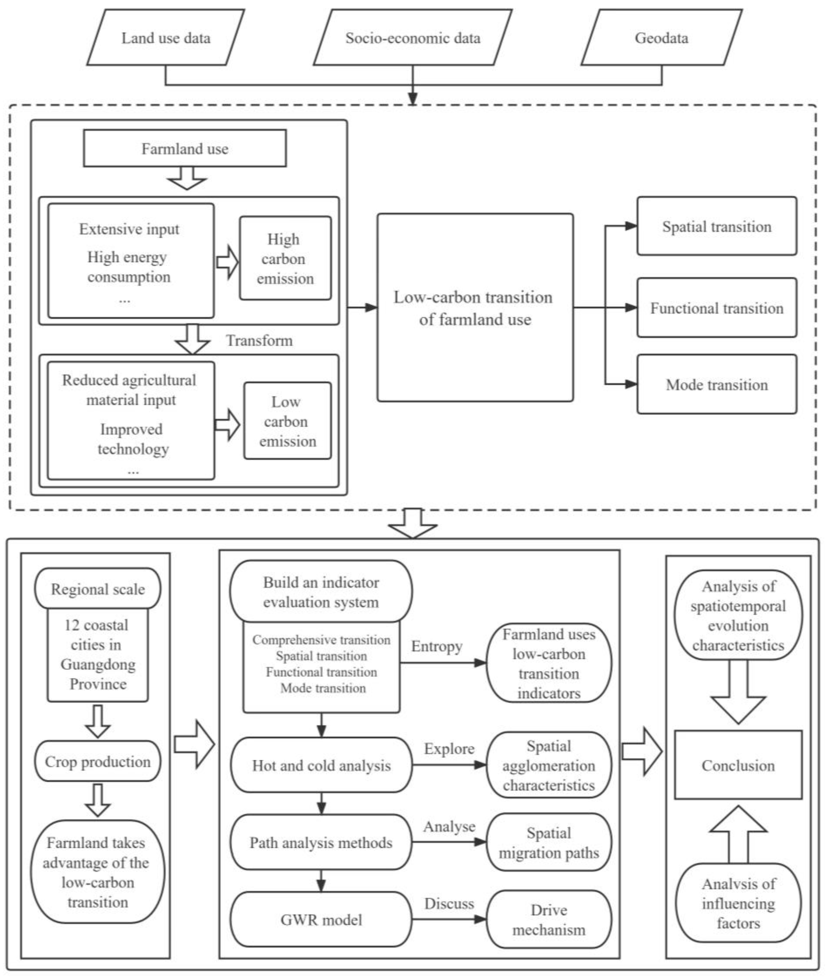
2. Materials and Methods
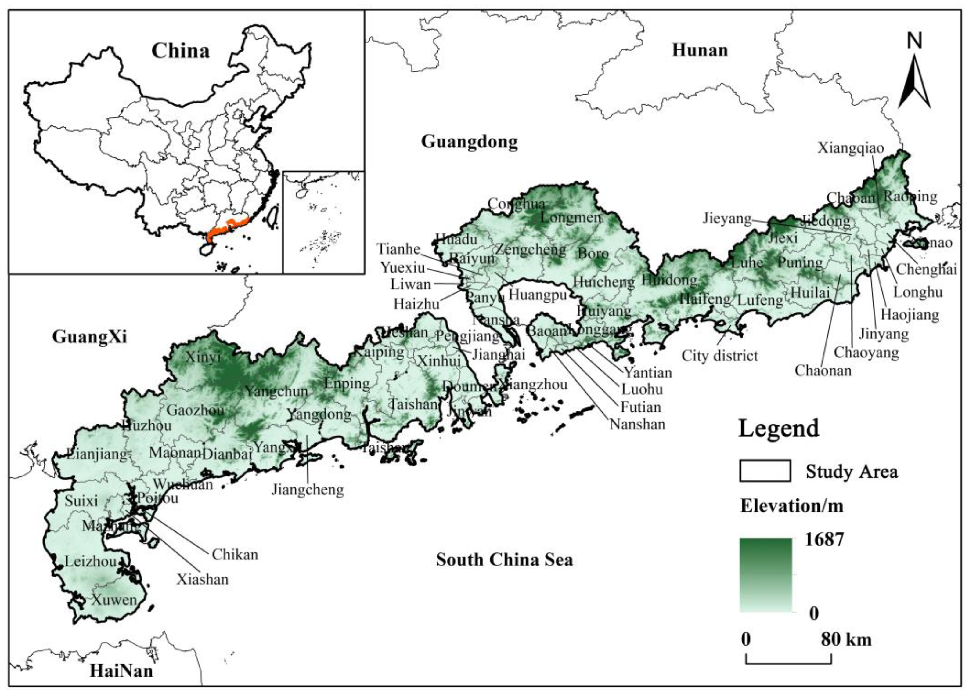
2.1. Study Area

The research area for this paper comprises the coastal cities of Guangdong Province in southeastern China, including the 12 prefecture–level cities of Guangzhou, Shenzhen, Zhuhai, Zhanjiang, Shantou, Chaozhou, Jieyang, Shanwei, Yangjiang, Maoming, Huizhou, and Jiangmen (Figure 1). The study units are the 69 counties and cities in the region. These cities are situated between 20°13′~24°14′ N and 109°40′~117°11′ E, with a total area of about 78,750 km2. Farmland comprises approximately 23,046 km2 as of the end of 2020, accounting for 29.42% of the total area of these cities (Resource and Environment Science and Data Center of the Chinese Academy of Sciences). Moreover, the annual grain production was more than 0.08 million tons. The gross domestic product (GDP) of the study area was CNY 78,341 billion as of the end of 2020, accounting for 70.73% and 7.76% of the GDP of Guangdong Province and the whole country, respectively (Statistics Bureau of Guangdong Province, National Bureau of Statistics of China, 2020). Among these cities, Guangzhou, Shenzhen, Zhuhai, Huizhou, and Jiangmen are distributed in the Pearl River Delta region and are the core area of economic development in the nation; they are also the core of the Guangdong–Hong Kong–Macao Greater Bay Area. Shantou, Chaozhou, Jieyang, and Shanwei border the Fujian Minnan region and have important economic development bases. Zhanjiang, Yangjiang, and Maoming have rich natural resources, developed agriculture, and the most fruit and vegetable production in China. Therefore, this region faces the challenge of coordinating economic development, food security, and low–carbon development.

2.2. Data Sources

Land use data: The farmland data used in this paper were obtained from Landset TM remote sensing image data (30 m resolution), provided by the Resource and Environment Science and Data Center of the Chinese Academy of Sciences (https://www.resdc.cn/) (accessed on 1 September 2021). The data were used to calculate indicators such as land settlement rate, farmland landscape fragmentation, average land value of plantation production, the replanting index, and carbon sequestration capacity.
Socio–economic data: The socio–economic data were obtained from China’s economic and social big data research platform (https://data.cnki.net/) (accessed on 17 December 2022), the Guangdong Statistical Yearbook (2001–2021), the Guangdong Rural Statistical Yearbook (2001–2021), and the statistical yearbooks of cities and counties. Missing data were calculated by the interpolation and moving average methods. The data were used to calculate the indicators of spatial transition, functional transition, mode transition, social factors, economic factors, and environmental factors.
Geodata: Administrative district boundaries and the Digital Elevation Model (DEM) (30 m resolution) were obtained from National Geomatics Center of China (http://www.ngcc.cn) (accessed on 25 December 2022).

2.3. Methods

This study investigated the spatial and temporal evolutionary trends of the LCTFU and its driving mechanisms. First, we constructed an indicator assessment system of the LCTFU and used entropy to measure indicators of the LCTFU. Second, we used cold and hot spot analysis to explore the spatial clustering characteristics of the LCTFU. At the same time, we analyzed the spatial migration path of the LCTFU using the path analysis method. Finally, a geographically weighted regression model (GWR) was used to explore the factors influencing the LCTFU (Figure 2).

2.3.1. Weights of Evaluation Indicators for the LCTFU

The weight of an evaluation index was assigned according to the relative degree of variance of its impact on the whole evaluation index system. An evaluation index with a larger variance, reflecting a smaller information entropy, was assigned a larger weight [34,35,36]. The higher the information entropy value of the selected evaluation indicators, the higher the degree of influence on the evaluation of the LCTFU. In order to eliminate the influence of different units on the selected evaluation indicators, a standardization process was used before calculating entropy.
The attribute matrix R was normalized, and the normalized value X = ( x i j ) m × n  was calculated as follows. The positive evaluation indicators selected in this study were normalized using the following formula:
X i j = x i j m i n x j m a x x j m i n x j
The negative evaluation indicator X i j was calculated by the formula:
X i j = m a x x i j x i j m a x x i j m i n x i j
where m is the number of evaluation indicators, n is the year, X i j  is the value corresponding to the j–th indicator in year i;   m a x x j denotes the maximum value of the j–th index; m i n x j denotes the minimum value of the j–th index; j = 1, 2,..., m; and i = 1, 2,..., n.
The weight p i j of the j–th indicator for the i–th year was calculated as follows:
p i j = X i j i = 1 m X i j
The indicator information for entropy E j (0 ≤ E j ≤ 1) was found using the following formula:
E i j = 1 ln n i = 1 n p i j ln p i j
where 1 ln n is the information entropy coefficient. The weights W i  of the indicators were calculated using:
W i = 1 E j n j = 1 n E j

2.3.2. Measurement of the LCTFU

Drawing on understanding of the LCTFU from previous studies, this study established a multilevel LCTFU evaluation index system with 3 subsystems, 6 factor layers, and 18 indicators (Table 1).
The spatial transition of farmland use considers its quantity form and spatial pattern. The quantity form includes farmland per capita (X1), land settlement rate (X2), and grain–to–economic ratio (X3). The farmland area per capita displays the amount of farmland use per capita [19,27]. The land settlement rate (X2) reflects the level of farmland use [28]. The grain–to–economic ratio (X3) shows changes in cultivation structure and can more accurately reflect the actual use rate of farmland [27,37]. The spatial pattern attribute is characterized by the landscape fragmentation of farmland (X4), which can reflect human disturbance to the landscape. Referring to the studies by Huang et al. [29] and Liang et al. [38], we chose farmland landscape fragmentation to reflect the spatial pattern of farmland.
The functional transition of farmland use considers its transition of production, living, and ecological functions. The production function can visually represent food production capacity, measured by the average land value of plantation production (X5), grain yield (X6), and replanting index (X7) [39,40]. The living function represents the ability of farmland to guarantee food security, employment level, and labor carrying capacity, measured by the guaranteed food per capita (X8), food quality and safety assurance (X9), share of agricultural employment (X10), and average land labor carrying capacity (X11) [41,42,43,44]. The ecological function represents the carrying capacity and resilience of farmland to the ecological environment, measured by fertilizer surface source pollution intensity (X12), carbon sequestration capacity (X13), proportion of farmland to ecological land (X14), and ecological carrying capacity of farmland per capita (X15) [45,46,47,48].
The low–carbon use of farmland focuses on enhancing the carbon sink function and reducing carbon emissions from farmland use. It incorporates the concept of “low–carbon” development into the transition of the farmland use mode by combining the realistic requirements of China’s “dual carbon” target. The mode transition of farmland refers to work by Wang et al. [49] to measure the degree of low–carbonization of farmland use in terms of the share of land–average carbon revenue and expenditure (X16).
The data were normalized to eliminate the effects of the metric and index scales. We used the entropy value method to calculate the weights of each indicator and calculated the low–carbon color transition index of farmland use with results from the product of each indicator weight and the standardized value of each indicator.

2.3.3. Cold and Hot Spot Analysis

The Gi∗(d) values were used to characterize the high–value areas (hot spot areas) and low–value areas (cold spot areas) of spatial units in the study area, and they revealed the spatial heterogeneity of the LCTFU. The hot spot areas were the clusters of county units with high farmland transition in a certain period, and the cold spot areas were the densely distributed areas of county units with low farmland transition. The formula is as follows:
G i ( d ) = j = 1 n W i j ( d ) X j j = 1 n X j
where d is the distance; W i j is the spatial weight between i and j in the study area; X j is the observed value of region j; and n is the number of study units.

2.3.4. Selection of Driving Factors of the LCTFU

The LCTFU results from the mutual constraints and joint action of the natural environment and socio–economic development in the region. Thus, this paper selected nine indicators as independent variables from the perspectives of social, economic, and environmental factors (Table 2).
Economic factors are the core factors affecting agricultural production and will ultimately affect the level of low–carbon technology in agricultural production [25]. Referring to the study by Ke et al. [50], we selected GDP per capita (Y4), fixed asset investment density (Y5), and percentage of agricultural GDP (Y6) to represent economic factors. Studies have demonstrated that urbanization rate (Y2) [50], population density (Y1) [27], and traffic density (Y3) [27] will affect the transition of farmland use. Thus, we selected Y1, Y2, and Y3 to indicate social factors. Natural factors can reflect the condition of farmland endowment, which affects the degree of farmland use and cultivation. Referring to the study by Zhang et al. [51], we selected DEM (Y7), forest coverage (Y8), and percentage of soil erosion (Y9) to represent environmental factors.

2.3.5. GWR Model

This study used a GWR model to explore contributors to the LCTFU in each county and region, and analyzed the importance and spatial distribution of each influencing factor. Traditional linear regression models (OLS model) are only global estimates of all samples and parameters and cannot account for the spatial relationships of the independent variables; parameter estimation with traditional linear regression models will no longer be applicable. Unlike traditional linear regression models (OLS model), GWR is a regression analysis tool for spatially variable coefficients. GWR can explore the non–stationarity of spatial relationships by incorporating spatial location information into the regression equation, which allows for the variation of parameters with their geographic location based on the variation of parameter estimates. The model structure is as follows:
y i = β 0 ( u i , v i ) + k β k ( u i , v i ) x i k + ε i
where y is the observed value; β 0 ( u i , v i ) is the regression coefficient at point I, indicating the degree of influence of the independent variable on the dependent variable; ( u i , v i ) represents the coordinates of the geographic center of the i–th sample spatial unit; β k ( u i , v i ) is the value of the continuous function β k ( u , v ) at sample spatial unit i; x i k denotes the value of the independent variable x k at point i; and ε is a normally distributed function with constant variance, representing the random error term.

3. Results

3.1. Spatial–Temporal Evolution Characteristics of the LCTFU

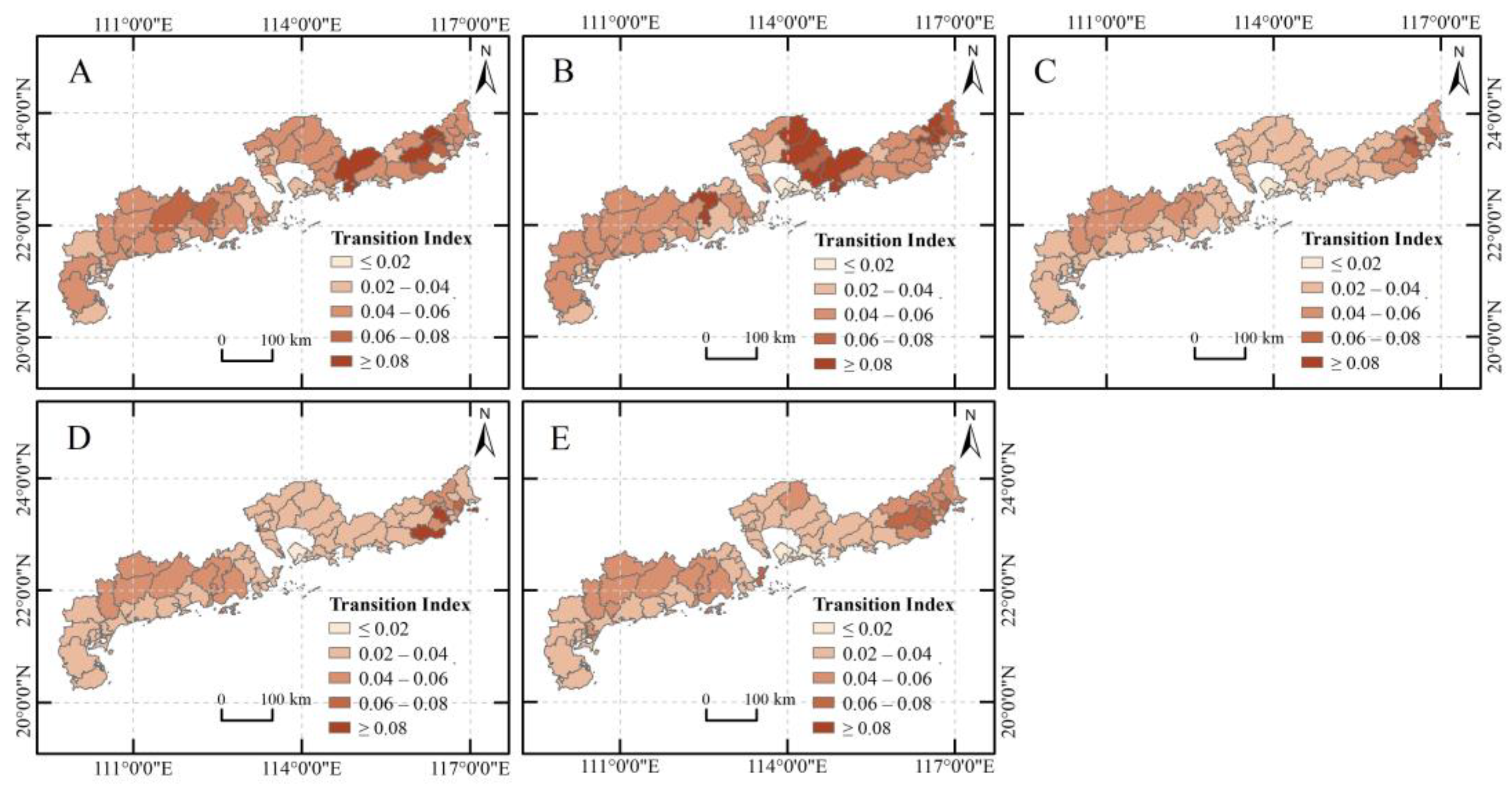
3.1.1. Comprehensive Transition

The comprehensive transition index of the LCTFU in the study area generally showed a trend of rising and then falling, and the average value of the composite transition index decreased by 0.15%, from 0.0449 in 2000 to 0.0372 in 2020. The comprehensive transition index varied among counties and districts, mainly fluctuating in [0.02, 0.08], with 39.13%, 24.64%, 43.48%, 39.13%, and 47.83% of the counties having a comprehensive transition index higher than the average value, indicating that most counties in coastal areas of Guangdong Province have a low level of comprehensive transition. The differences in the LCTFU among the counties and districts were narrowing. In terms of their spatial distribution, the overall comprehensive transition index of the study area from 2000 to 2020 varied greatly toward the edges, but little in the center of the study area. The areas with high values on this index were concentrated mainly in the eastern and western parts of the study area (i.e., the counties under the jurisdiction of Maoming, Yangjiang, Jiangmen, Jieyang, Shantou, and Chaozhou), which represent the counties with lower levels of economic and social development. The areas with low values of this index were concentrated in the center of study area; they were counties within the Guangzhou, Shenzhen, and Zhuhai urban agglomerations of the Pearl River Delta, a highly developed socio–economic coastal region of China (Figure 3).

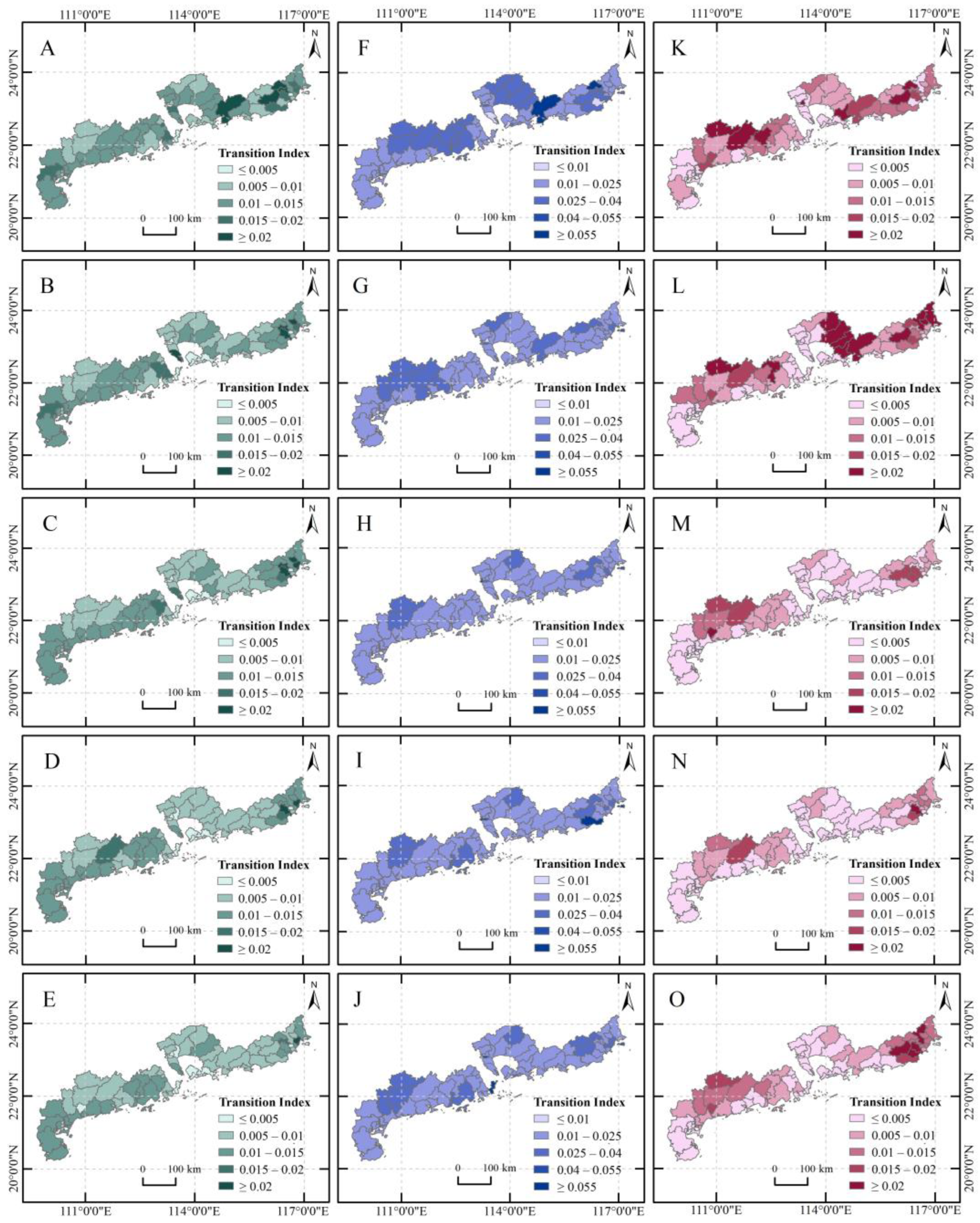
3.1.2. Spatial Transition

The spatial transition index generally decreased, moving from 0.0125 in 2000 to 0.0079 in 2020, a decline of 0.09%. This trend may be attributed to the significant decrease in the amount of farmland from 2000 to 2020 and a slight downward trend in the change in landscape pattern, the combined effect of which led to a decrease in the spatial transition of farmland (Figure 4). Over the past 20 years, the rate of change in the spatial transition index was 0.02%, indicating that the differences in the spatial transition among counties and regions have been narrowing. The spatial transition of high–value areas was distributed mainly in the west and east, and that of the low–value areas was distributed mainly in the north. Since the spatial transition was obviously constrained by farmland, fragmentation of the arable landscape, and topography, counties with contiguous farmland, low elevation, and flatter topography in the western and eastern parts of the study area had higher spatial transition index values, while most counties in the north had high elevation and smaller farmland areas and aggregation, contributing to their lower spatial transition index.

3.1.3. Functional Transition

Overall, the functional transition index decreased from 0.0242 to 0.0225 between 2000 and 2020, which is a small change. During the study period, the transition index capturing the production function of farmland in the study area increased from 0.0067 to 0.0088, and the transition indexes for the living and ecological functions of farmland decreased from 0.0102 and 0.0083 to 0.0086 and 0.0069, respectively (Figure 4). The increase in average grain yield and average land value of plantation production increased in the production function of farmland, while the decrease in per capita food security and agricultural workforce corresponded to a decreased living function of farmland. Still, the intensity of fertilizer surface source pollution decreased from 340 km/hm2 to 282 km/hm2, and the continuous decrease in the carbon sequestration capacity and the ecological carrying capacity of farmland per capita led to decreased farmland ecological function. The functional transition indexes of the counties in the study area were generally low. The high–value areas of the function transition index were scattered in counties with higher topography in the north of the study area, and the number of high–value areas was decreasing. In contrast, the low–value areas were distributed widely in the center and west, with some counties in the east. In the northern part of the study area, due to the influence of geographical location and socio–economic development, the ecological function of farmland was strong, the proportion of modern agriculture was low, the efficiency of agricultural production was low, and a large amount of labor outflow led to the weakening of the production and living functions of farmland.

3.1.4. Mode Transition

The mode transition index depicted clear spatial differences, with a general trend of increasing and then decreasing. The mean value of mode transition increased from 0.0083 in 2000 to 0.0203 in 2005 and then decreased to 0.0068 in 2020 (Figure 4). The high–value areas were located mainly in the western and eastern parts of the study area (i.e., counties under the jurisdictions of Maoming, Yangjiang, Huizhou, Jieyang, Shantou, and Chaozhou), where they were characterized by a low level of economic development and a high carbon sequestration capacity of farmland. The low–value areas were located mainly in the center of the study area, including the counties under the jurisdictions of Guangzhou, Shenzhen, and Zhuhai, which were areas with high economic development characterized by a small amount of farmland and weak carbon sequestration capacity. The high–value areas of the mode transition index increased from 2000 to 2005, and then decreased from 2005 to 2020.

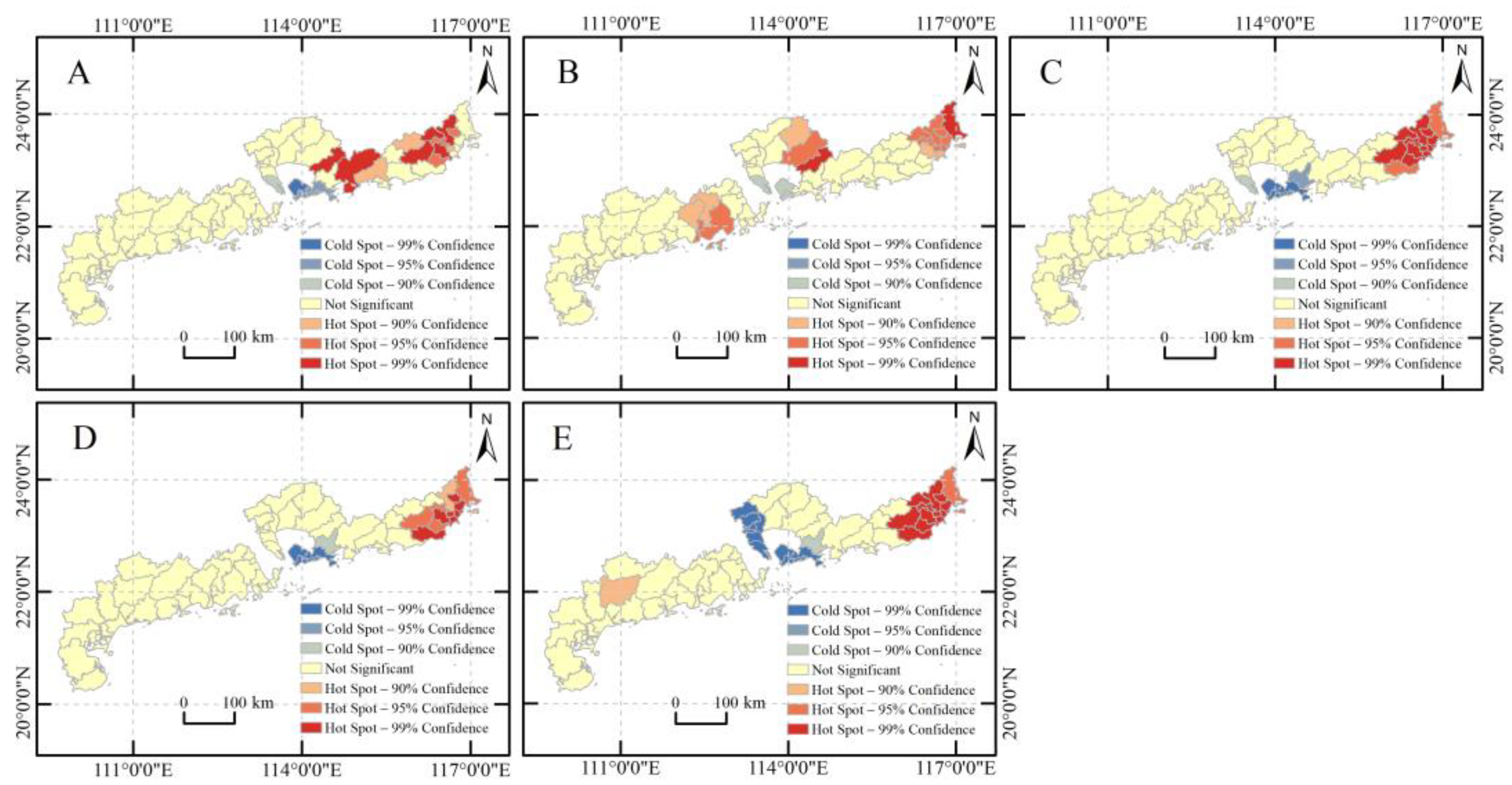
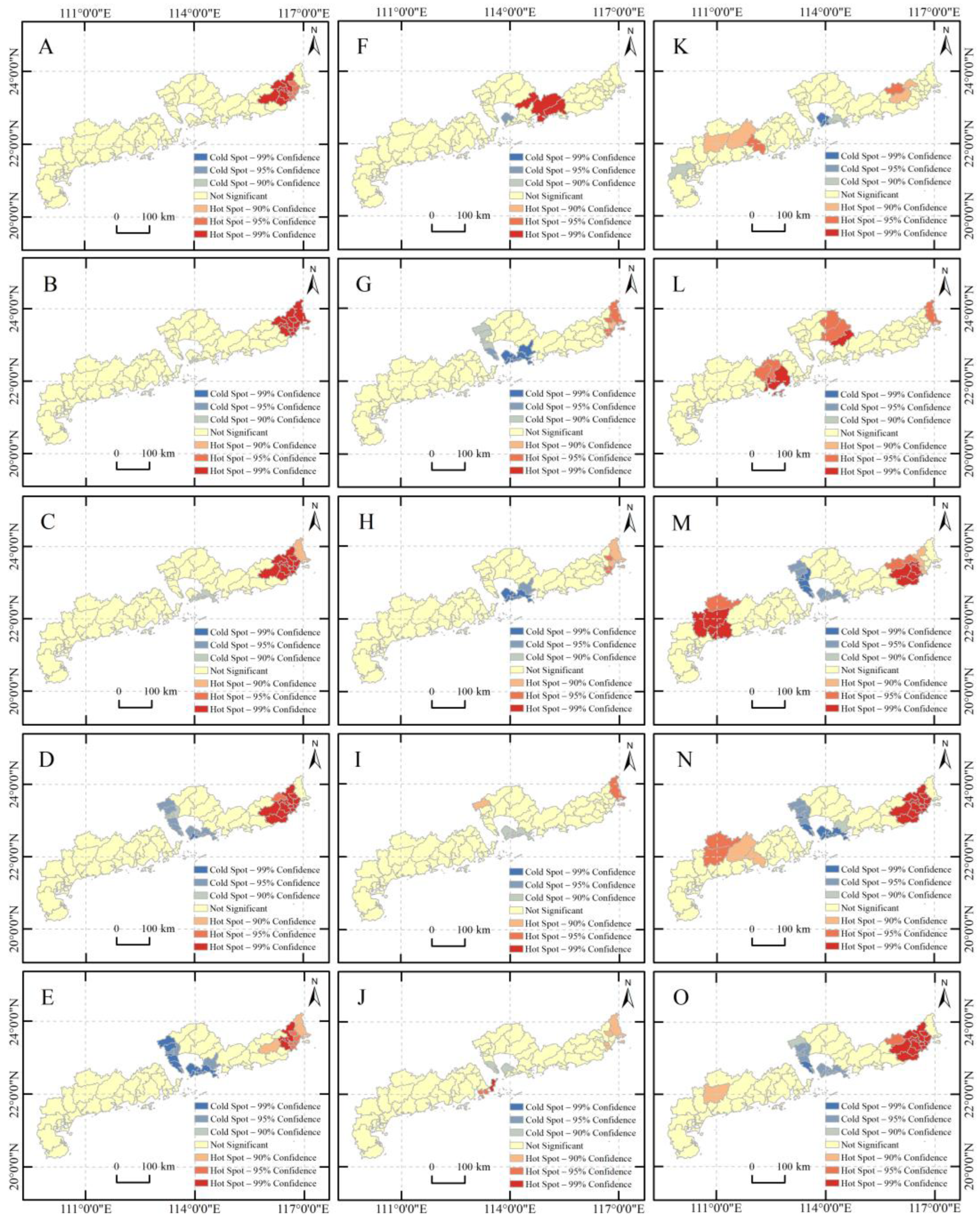
3.2. Spatial Clustering Characteristics of the LCTFU

For each stage, in 2000, 2010, 2015, and 2020, the Getis–Ord Gi* tool was used to derive the significant cold spot and hot spot areas of the spatial distribution of the four indexes of comprehensive, spatial, functional, and mode transition and the cold and hot spot distribution of the four indexes (Figure 5 and Figure 6). The four LCTFU indexes in coastal counties and districts of Guangdong Province had positive clustering effects in terms of their spatial distribution. The high–value (hot spot) areas of the comprehensive transition index were concentrated in counties within Huizhou, Jieyang, Jiangmen, Shantou, and Chaozhou, and the eastern counties of the study area maintained more stable hot spots. The low–value (cold spot) areas were concentrated in counties within Guangzhou and Shenzhen, and the cold spot areas were becoming more prominent.
The high–value (hot spot) areas of the spatial transition index were concentrated in the counties within Jieyang, Shantou, and Chaozhou in the eastern part of the study area. The hot spot areas in the eastern counties showed strongly significant differences from 2000 to 2015, although they weakened in 2020. Due to the advantages of the amount of farmland and grain production in these counties, the population was relatively small. Low–value (cold spot) areas were concentrated in counties within Guangzhou and Shenzhen, in the center of the study area, areas with small amounts of farmland, dense populations, and high economic and social development. The latter has led to a continuing reduction in farmland population density and a subsequent increase in cold spots. Most of the counties in the study area showed insignificant functional transition indexes, and the high–value (hot spot) areas of the functional transition indexes were concentrated in a small number of counties in Huizhou (in 2000, stronger significance), Chaozhou (after 2005, weaker significance), and Zhuhai. Low–value (cold spot) areas were concentrated in counties within Guangzhou and Shenzhen in the center of study area. The number of counties with low–value areas increased and became more significant from 2000 to 2010, but gradually diminished after 2015. The high–value (hot spot) areas of the mode transition index were concentrated in the counties of Maoming, Huizhou, Jieyang, and Shantou, with the western areas concentrated mainly in Maoming. In the east, the high–value areas showed an expanding trend, and the significance continued to increase after 2010. The low–value (cold spot) areas were concentrated in counties within Guangzhou and Shenzhen, in the center of study area; their significance weakened and then gradually increased.
According to the results presented in Figure 4 and Figure 5, the four transitions of the high–high agglomeration areas were mainly in the eastern part, and the low–low agglomeration areas were mainly in the center part of the study region. This distribution was primarily due to differences in national policies, economic development levels, and topography. High–high agglomeration areas were mostly areas with high topography, low economic development, and poor agricultural production technology, while low–low agglomeration areas were the core cities of the Pearl River Delta and the Guangdong–Hong Kong–Macao Greater Bay Area in China, important engines of national economic development. The trend of new construction occupying continuously flat farmland is expanding, and farmland fragmentation is high, making the various transitions of farmland somewhat constrained.

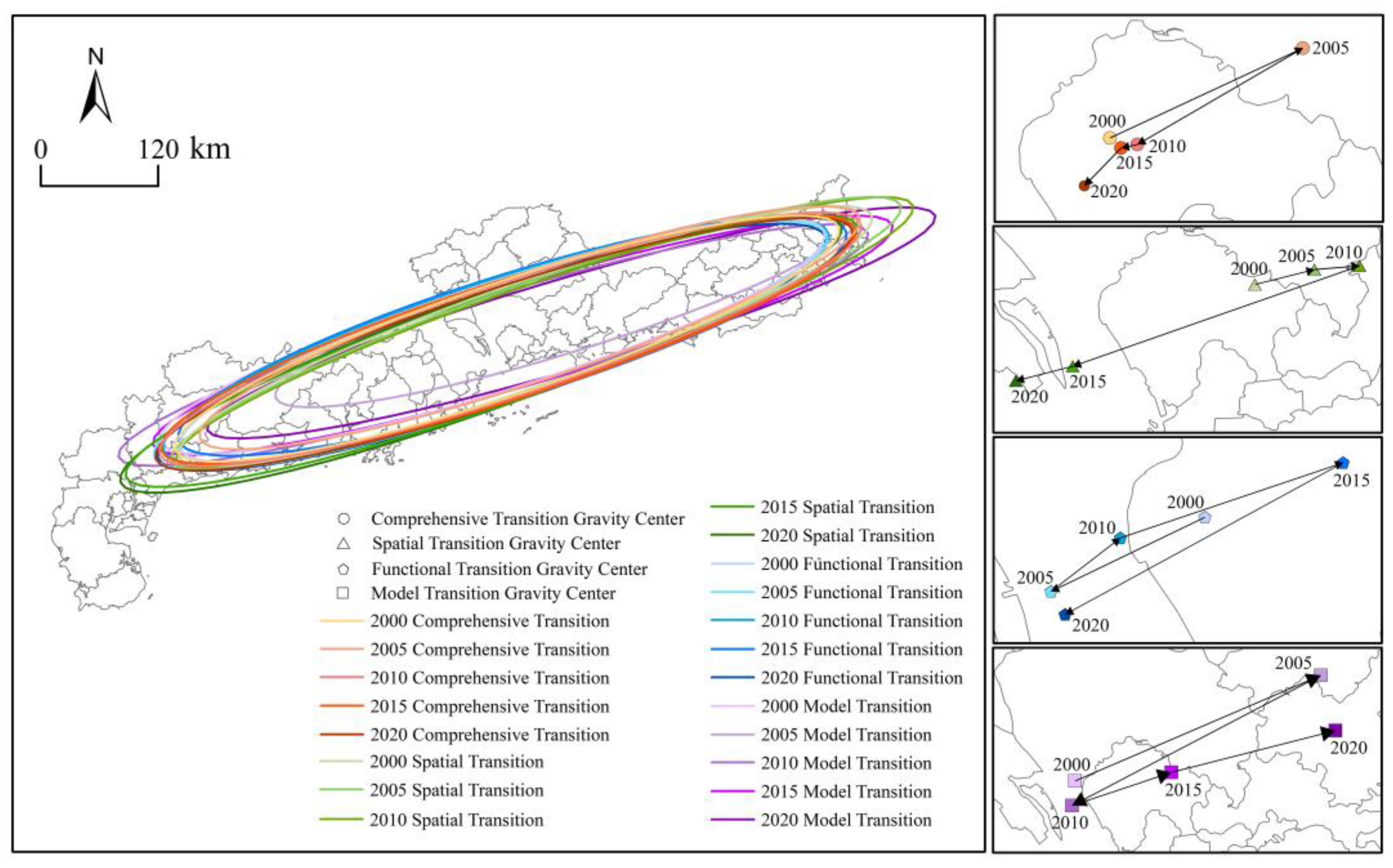
3.3. Path Analysis of the LCTFU

The spatial migration path of the farmland use transition in the study area was analyzed using ArcGIS 10.8 software. Based on the elliptical azimuth tan θ parameter, the spatial migration of the farmland use transition from 2000 to 2020 showed a northeast–southwest pattern, with a continuous contraction in the north–south direction, a continuous translation in the east–west direction, and a tendency to drift to the southwest (Figure 7).
The transition center of the gravity migration path from the standard deviation ellipse center was not particularly significant during the 20–year period, and the ellipse center was still in the middle of the region in 2020. The center of gravity of the comprehensive transition moved 6.44 km, that of the spatial transition moved 45.52 km, functional transition moved 12.18 km, and mode transition moved 74.59 km. The comprehensive transition center of gravity movement speed decreased from 4.85 km/year to 0.74 km/year, spatial transition decreased from 2.14 km/year to 2.07 km/year, functional transition decreased and then increased to 4.51 km/year, and mode transition decreased from 15.15 km/year to 9.51 km/year. In addition, the centers of gravity of the comprehensive transition and functional transition have been in Baoan District, Shenzhen; that of the spatial transition was transferred from Baoan District to Nansha District, Guangzhou, after 2015; and the pattern transition was transferred to Huicheng District, Huizhou, in 2005, back to Baoan District in 2010, and then to Huiyang District, Huizhou, in 2020. From the degree of coverage of the standard deviation ellipse, the spatial distribution of the LCTFU in the study area during the 20–year period examined showed an expansion that was continuously fluctuating. The directional changes of the spatial transition and comprehensive transition were basically the same. The functional transition generally expanded to the southwest, and the pattern transition generally showed a weaker expansion trend. Based on the ellipse’s spatial location, the geographical range contained more cities, the main body of the ellipse was in the central location of the study area, and the overall spatial pattern was C–shaped, indicating that there were differences in the transition of farmland use across the study area, and the transition intensity of the central counties was higher than that of other regions.

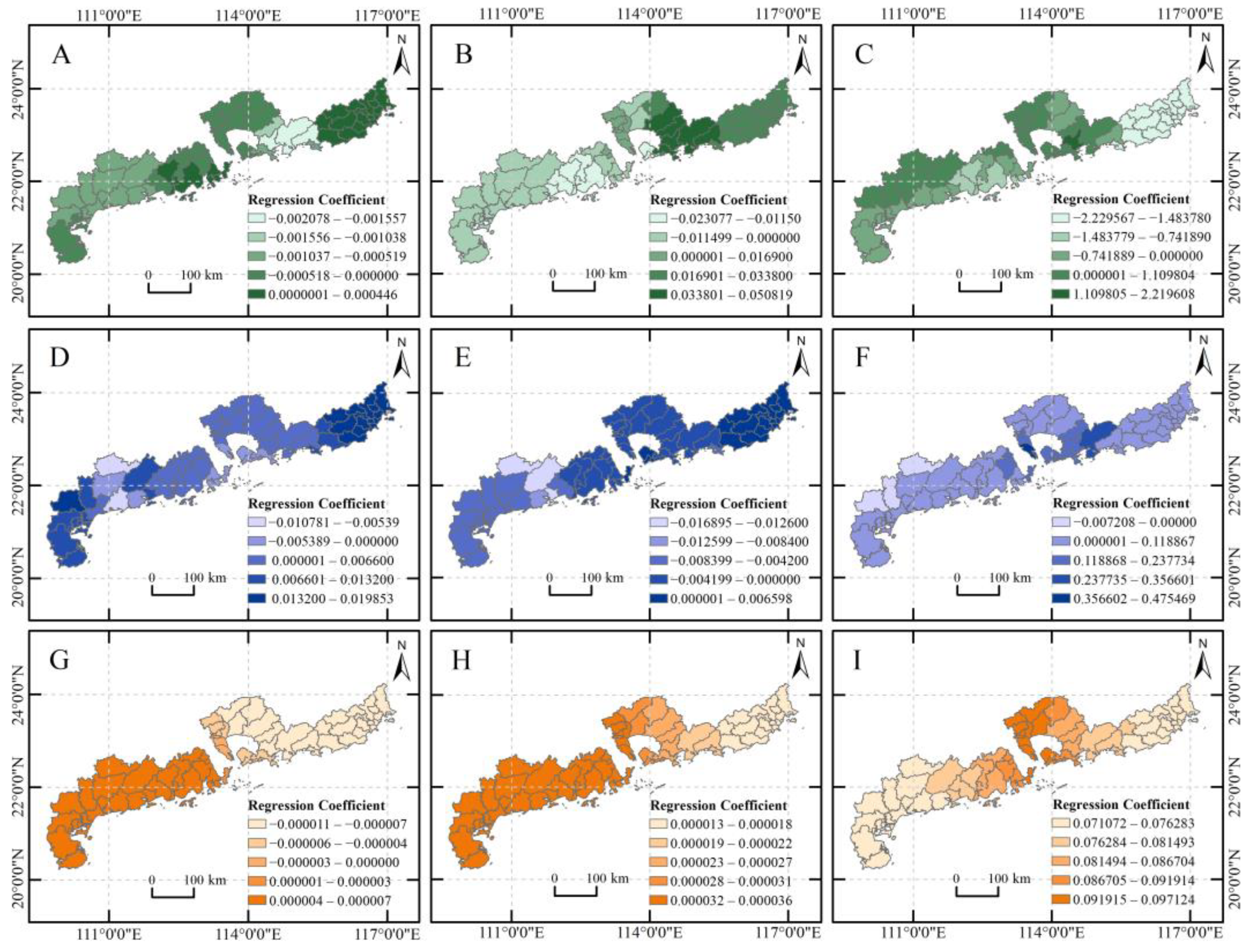
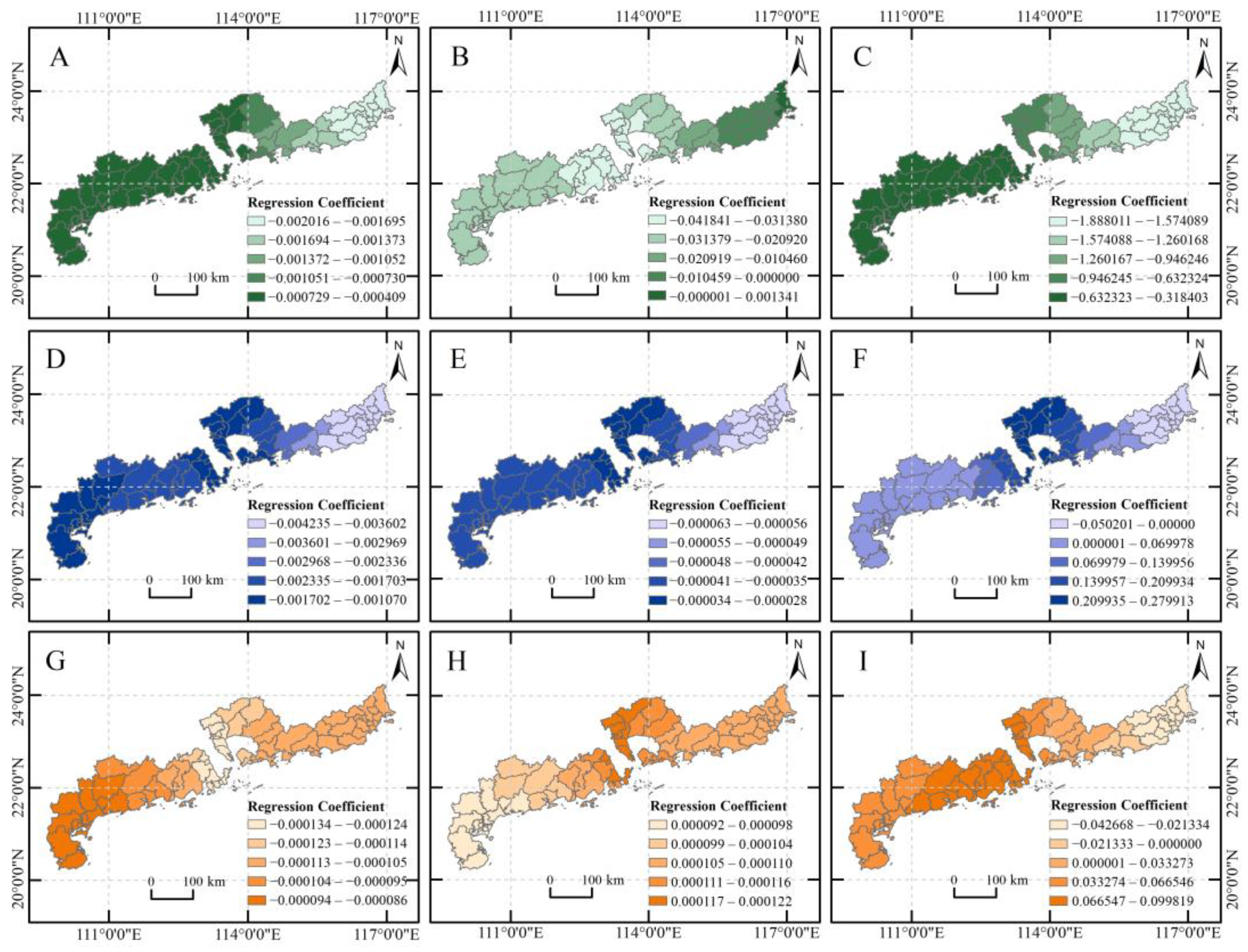
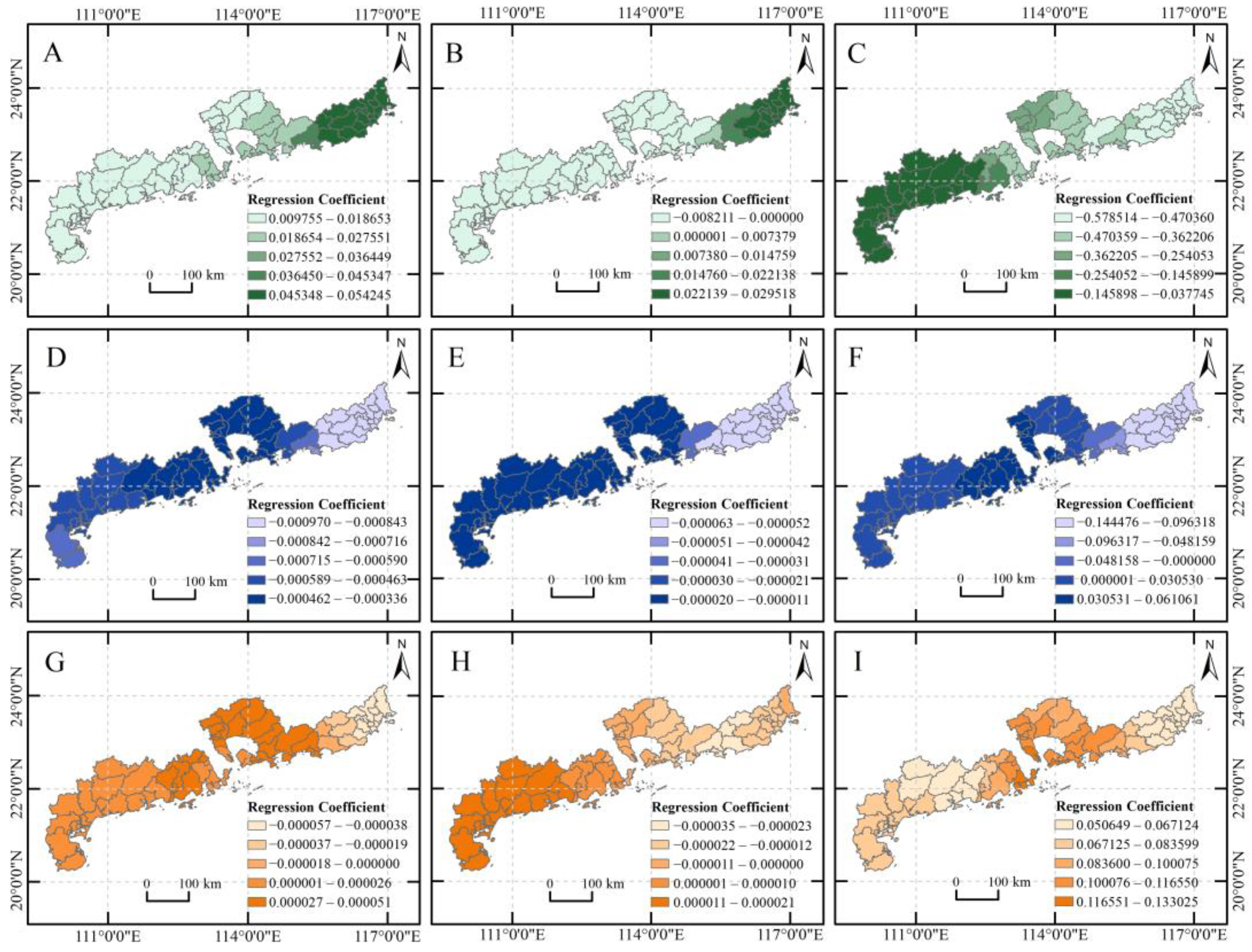
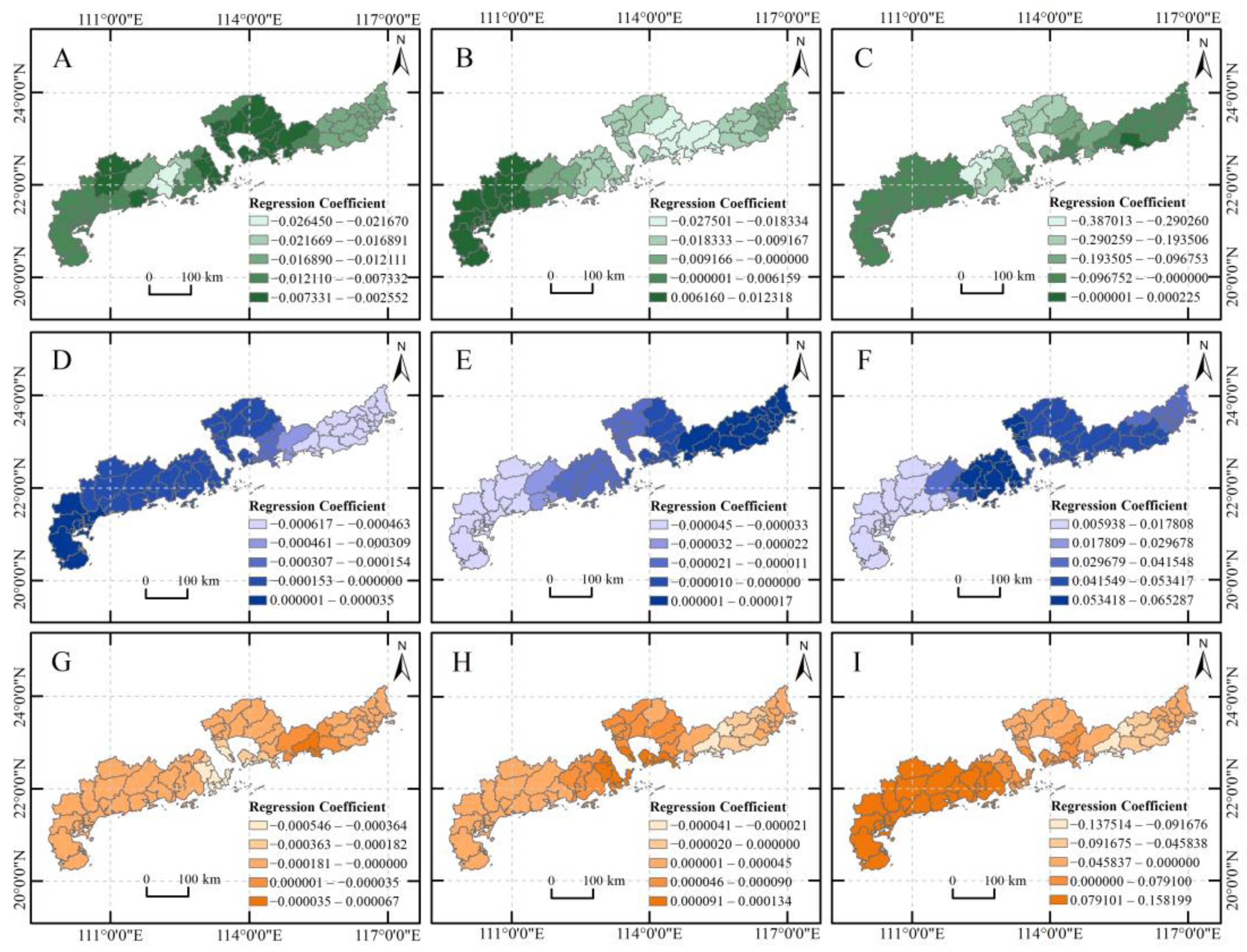
3.4. Analysis of the Driving Factors of the LCTFU

This paper identifies the driving mechanisms based on social, economic, and environmental factors, and used the GWR model to measure the regression coefficients of each influencing factor from 2000 to 2020. Spatial autocorrelation analysis of the variables was required before using the GWR model. ArcGIS software was used to calculate the global Moran’s I indexes of the variables and test their significance. The Moran’s I index of each variable was high, all were greater than 0, and the p–value was much less than 1%, passing the significance level test of 99%. The R2 values of the GWR model ranged from 0.179 to 0.664, and the AICc values ranged from −190.895 to −401.150 for each year, indicating that the model fits better and has strong explanatory power (Table 3).
As for social factors, the regression coefficients for population density and urbanization rate fluctuated [−0.04, 0.05], indicating that the spatial differences between population density and urbanization rate were significant. Both population density and urbanization rate had positive and negative effects on the LCTFU. In 2000–2005, the regression coefficients on population density were mostly negative, the number of positive areas was small, and the changes were weak. In 2010, the regression coefficients for population density were all positive, and population density had a positive impact on the LCTFU in the study area, with the eastern region showing the strongest influence. From 2015 to 2020, the coefficients for population density were all negative, and population density had a negative impact on the LCTFU. From 2000 to 2010, the number of areas with positive values for urbanization rate were distributed mainly in the east of the study area. The coefficients of the urbanization rate in the center and west of the study area were negative, indicating that the urbanization rate had a positive influence on the LCTFU in the eastern study area and a negative influence on the LCTFU in the central and western parts of the study area. From 2015 to 2020, the influence of the urbanization rate on the LCTFU gradually decreased from the western part of the study area to the east, indicating that the urbanization rate negatively influenced the LCTFU in the study area and gradually decreased. From 2000 to 2010, the regression coefficient for traffic density fluctuated [−2.23, 2.21]. In 2000, the positive values of traffic density were distributed mainly in the center and the west. The positive values were larger and more widely distributed, while the negative values were mainly in the east, showing an overall distribution pattern from high in the center and west to low in the east. After 2005, the regression coefficients of traffic density were mostly negative, and the negative values were larger, indicating that traffic density mainly negatively influenced the LCTFU of each region in the study area. During the study period, population density and traffic density mainly negatively affected the LCTFU in all regions of the study area, with weak positive effects. Urbanization rate negatively affected the LCTFU in the center and west, and had positive effects in the east before turning to negative effects. Socio–economic development, population density, urbanization rate, and traffic density have increased to a certain extent in coastal areas of Guangdong Province. Population concentration, high urbanization level, and high traffic density will expand the amount of construction land and decrease the amount of farmland, the area of farmland patches, and the degree of concentration. These changes will lower the level of farmland production function and spatial transition, which will negatively influence the study area’s LCTFU to some degree. Urbanization will cause many rural laborers to move to highly developed areas in the center of the study area. This migration will increase the population density and demand for agricultural products in the center of the study area and stimulate the flow of farmland, agricultural modernization, and agricultural scale operation in the western and eastern parts of the study area. The amount of chemical fertilizers and pesticides used per unit area of farmland would decrease, improving the production and ecological functions of farmland in the western and eastern parts of the study area, which will positively impact functional transition to some degree.
The coefficients for regional economic factors fluctuated [−0.14, 0.47], indicating that economic development had both positive and negative effects on the LCTFU. Between 2000 and 2010, the negative effects of GDP per capita and fixed asset investment density gradually weakened, and the positive effects of the gross agricultural product ratio gradually increased from west to east, while the number of counties with positive effects grew. The ratio of the LCTFU gradually increased, and the number of counties with positive effects did not increase much. For 2015–2020, the regression coefficients for each economic factor were generally positive, and each had positive effects on the LCTFU. The continuous expansion of urban and rural construction land, due to economic growth and the over–exploitation of resources, led to a sharp decrease in the “quantity” and “quality” of farmland resources and inhibited the LCTFU. This trend changed in 2015, when regional economic development became an important factor in promoting the LCTFU. With the continuous socio–economic development of coastal areas in Guangdong Province, local governments increased investment in fixed assets, such as agricultural irrigation facilities and the construction of high–quality basic farmland. This investment promoted the large–scale operation of farmland and agricultural mechanization and modernization, and facilitated the LCTFU.
Additionally, the environmental impact coefficients fluctuated between [−0.14, 0.15], with significant spatial heterogeneity. There was a positive distribution of influence mainly in the west and east, and a weak positive influence in the central region. Environmental factors in the northern part of the study area, such as high topography, large forest coverage, and strong farmland ecological functions but weak production and living functions, significantly positively influenced the LCTFU in the north. Due to the high and concentrated precipitation in the coastal areas of Guangdong Province, natural disasters significantly impacted land use. Jiexi County, Puning City, Luhe County, and Gaocheng City, in the western and eastern parts of the study area, were classified as key erosion control areas, and the frequent soil erosion damaged the farmland system, as well as the production, living, and ecological functions of farmland. In contrast, due to the high socio–economic level of the central region, the quantity of farmland was small. The high fragmentation of farmland here prompted the simultaneous reduction in the spatial and functional transition, which had a certain constraining effect on the LCTFU (Figure 8, Figure 9, Figure 10, Figure 11 and Figure 12).

4. Discussion

4.1. Potential Reasons for the LCTFU

Overall, we found that the LCTFU is at low levels from 2000 to 2020. Similarly, Ke et al. [50] explored LCTFU in Hubei Province from 2000 to 2019, and found that the LCTFU is relatively low, but higher than that in coastal areas of Guangdong Province. This might be because Hubei is located in Jianghan Plain, where the degree of farmland fragmentation is relatively low [52]. In contrast, the spatial differences in the distribution of farmland in coastal areas of Guangdong Province are relatively large, and the extent of farmland fragmentation is generally high [49]. As for the functional transition, our results indicated that the transition of ecological function and living function of farmland use is continually decreasing, while that of the production function generally increased during the study period. The coastal areas of Guangdong are developed rural areas with a large proportion of non–agricultural employees, and the income of farmers mainly comes from non–agricultural industries. The livelihood security function of farmland is continuously weakened, while the production function is continuously enhanced with the extensive application of green agricultural technology [53]. As for the mode transition, the high–value areas of the mode transition index increased from 2000 to 2005, and then decreased from 2005 to 2020. This might be due to rapid urbanization development during 2005–2020 in the coastal areas of Guangdong Province, which has accelerated the expansion of urban construction land, eroded farmland, and ultimately led to a reduction in carbon sinks [54].
For the driving factors of LCTFU, we found that the LCTFU is the result of a combination of the social, economic, and environmental factors in the county, and that social factors have the greatest impact on the LCTFU. This view has been confirmed by scholars who have analyzed the LCTFU and its driving factors in Hubei Province, an inland region, and the results of the study pointed out that economic growth has been identified to have a more significant impact on the farmland use transition [28]. Among social factors, urbanization plays an important role. Urbanization causes contiguous farmland to be converted to urban construction land, leading to a decrease in the area of arable patches and an increase in the fragmentation of farmland [55]. These changes ultimately lead to a lower level of spatial transition. Some scholars have pointed out that increasing urbanization has led agricultural labor to shift to secondary and tertiary industries in economically developed areas, leading to a decrease in rural population density, and the extent of farmers’ use of farmland can be significantly weakened [56], thereby constraining the functional transition of farmland. In addition, economic factors have both positive and negative impacts on the LCTFU in different stages. This result is consistent with the results of Chen et al. [47]. The industrial–technological progress induced by economic development can promote the transformation of agricultural production methods and the innovation of production technology, which in turn induces the farmland use transition to the direction of relative quality improvement [57,58]. Our study also found that natural factors, such as DEM, have significantly influenced LCTFU. This result is confirmed by Chen et al. [47], as they found that DEM has significantly impacted the spatial pattern of cultivated land use.

4.2. Policy Implications

In order to achieve sustainable regional economic, social development, and “double carbon” goals, as well as ensure food security, each region should identify the leading factors influencing the LCTFU. Regional differences in the level of the LCTFU and farmland use patterns and methods should be accounted for when formulating targeted and timely policies and measures for farmland use. Our research showed a continuous decrease in farmland area in the study area from 2000 to 2020, along with a decrease in the area of farmland patches and the agglomeration level. In order to optimize agricultural, ecological, and urban spaces, local governments should develop territorial spatial planning, implement comprehensive land preparation projects, and improve the productive and ecological functions of farmland.
This study also reveals regional differences in the level of the LCTFU in the coastal areas of Guangdong Province. Highly developed economic areas have a lower level of LCTFU due to the greater demand for land for urban construction and the urban population’s higher consumer demands. Therefore, controlling the supply of urban construction land, fully exploiting the potential of urban low–utility land, and implementing urban low–utility land consolidation projects to improve land use efficiency and strengthen farmland protection are crucial. For relatively economically underdeveloped western and eastern regions, the main goal should be to enhance various farmland functions. Localities should develop green agriculture from a low–carbon perspective, innovate agricultural ecological compensation mechanisms, and absorb part of the agricultural labor force by introducing a series of agricultural subsidies and protection policies. Furthermore, promoting the transfer of farmland, agricultural modernization, and large–scale agricultural operations will help to improve farmland productivity and achieve intensive, efficient, and low–carbon use of farmland.

4.3. Limitations and Prospects

(1)
This paper aims to develop a comprehensive evaluation system for the LCTFU using a “spatial–functional–mode” approach, combining quantitative and qualitative perspectives. However, since farmland use is a complex and long–term process, various factors affecting the LCTFU may not be captured in the evaluation system presented in this paper. Future research may consider adding indicators such as the level of technological innovation in farmland carbon sequestration and emission reduction, and the level of ecological management of farmland.
(2)
This paper focuses primarily on the social, economic, and environmental factors that affect the LCTFU, but policy factors should also be considered in future studies. However, policy factors may be challenging to analyze quantitatively.
(3)
The paper employs a geographically weighted regression (GWR) model to explore the influencing factors of the LCTFU, providing useful insights for future research. One advantage of the GWR model is its ability to visualize the spatial heterogeneity of research results. However, the GWR model is a linear model, and it can only quantify the degree of influence of a single influencing factor indicator on the LCTFU. It cannot quantify the degree of influence of two or more influencing factor indicators on the LCTFU.

5. Conclusions

This study reveals the spatial–temporal evolution patterns and driving factors of the LCTFU in coastal areas of Guangdong Province by constructing a “spatial–functional–mode transition” index system and adopting a GWR model. Based on the analysis and findings, the following conclusions were drawn:
(1)
The comprehensive, spatial, and functional transitions, as well as the mode transition of farmland use in coastal areas of Guangdong Province decreased overall from 2000 to 2020, and the level of LCTFU in most counties is low. Spatially, the LCTFU in the study area generally exhibits a high–low–high spatial distribution pattern, with high levels of LCTFU in the east and west, and low levels in the center.
(2)
The hot spots of the comprehensive, spatial, functional, and mode transitions are distributed mainly in the eastern part of the study area, and the cold spots are concentrated in the central region of the study area, which was basically consistent with the spatial distribution of the high and low value areas of the LCTFU in the study area.
(3)
The center of gravity of LCTFU moved from northeast to southwest during the study period; the LCTFU shows a trend of continuous fluctuation and expansion in the physical space, with a noticeable spatial spillover effect.
(4)
The evolution of the LCTFU is driven by the combined effects of social, economic, and environmental factors, with social factors being the strongest driver.

Author Contributions

Conceptualization, X.H. and Y.W.; methodology, X.H. and W.L.; software, X.H. and W.L.; validation, X.H., Y.W. and X.Z.; investigation, Z.W., Q.Y., and X.Z.; data curation, X.H., Q.Y. and W.L.; writing—original draft preparation, X.H. and Y.W.; writing—review and editing, X.H., Y.W. and X.Z.; visualization, X.H and W.L.; supervision, Y.W. All authors have read and agreed to the published version of the manuscript.

Funding

This research was supported by the Youth Foundation of the School of Public Administration, China University of Geosciences (No. CUGGG–2201), the “CUG Scholar” Scientific Research Funds at the China University of Geosciences (Wuhan) (Project No. 2022128), and the Humanities and Social Sciences Foundation of Guizhou University (No. GDYB2022049).

Data Availability Statement

Not applicable.

Acknowledgments

The authors are particularly grateful to all researchers for providing data support for this study.

Conflicts of Interest

The authors declare no conflict of interest.

References

  1. Hong, C.; Burney, J.A.; Pongratz, J.; Nabel, J.; Mueller, N.D.; Jackson, R.B.; Davis, S.J. Global and regional drivers of land–use emissions in 1961–2017. Nature 2021, 589, 554–561. [Google Scholar] [CrossRef] [PubMed]
  2. Searchinger, T.D.; Wirsenius, S.; Beringer, T.; Dumas, P. Assessing the efficiency of changes in land use for mitigating climate change. Nature 2018, 564, 249–253. [Google Scholar] [CrossRef]
  3. Porter, J.R.; Challinor, A.J.; Henriksen, C.B.; Howden, S.M. Invited review: Intergovernmental Panel on Climate Change, agriculture, and food—A case of shifting cultivation and history. Glob. Chang. Biol. 2019, 25, 2518–2529. [Google Scholar] [CrossRef]
  4. Montzka, S.A.; Dlugokencky, E.J.; Butler, J.H. Non–CO2 greenhouse gases and climate change. Nature 2011, 476, 43–50. [Google Scholar] [CrossRef] [PubMed]
  5. Zeng, N.; Zhao, F.; Collatz, G.J.; Kalnay, E. Agricultural green revolution as a driver of increasing atmospheric CO2 seasonal amplitude. Nature 2014, 515, 394–397. [Google Scholar] [CrossRef]
  6. Tubiello, F.N.; Fischer, G. Reducing climate change impacts on agriculture: Global and regional effects of mitigation, 2000–2080. Technol. Forecast. Soc. Chang. 2007, 74, 1030–1056. [Google Scholar] [CrossRef]
  7. Vermeulen, S.J.; Aggarwal, P.K.; Ainslie, A.; Angelone, B.M. Options for support to agriculture and food security under climate change. Environ. Sci. Policy 2012, 15, 136–144. [Google Scholar] [CrossRef]
  8. Wiebe, K.; Lotze–Campen, H.; Sands, R.; Tabeau, A.; van der Mensbrugghe, D. Climate change impacts on agriculture in 2050 under a range of plausible socioeconomic and emissions scenarios. Environ. Res. Lett. 2015, 10, 085010. [Google Scholar] [CrossRef]
  9. Chuan Liao, K.N.; Sullivan, J.A.; Brown, D.G. Carbon emissions from the global land rush and potential mitigation. Nat. Food 2021, 2, 15–18. [Google Scholar] [CrossRef] [PubMed]
  10. Lu, X.; Kuang, B.; Li, J.; Han, J.; Zhang, Z. Dynamic evolution of regional discrepancies in carbon emissions from agricultural land utilization: Evidence from Chinese provincial data. Sustainability 2018, 10, 552. [Google Scholar] [CrossRef]
  11. Koondhar, M.A.; Aziz, N.; Tan, Z.; Yang, S.; Raza Abbasi, K.; Kong, R. Green growth of cereal food production under the constraints of agricultural carbon emissions: A new insights from ARDL and VECM models. Sustain. Energy Technol. Assess. 2021, 47, 101452. [Google Scholar] [CrossRef]
  12. Mallapaty, S. How China could be carbon neutral by mid–century. Nature 2020, 586, 482–483. [Google Scholar] [CrossRef] [PubMed]
  13. Zhou, Y.; Zou, S.; Duan, W.; Chen, Y.; Takara, K.; Di, Y. Analysis of energy carbon emissions from agroecosystems in Tarim River Basin, China: A pathway to achieve carbon neutrality. Appl. Energy 2022, 325, 119842. [Google Scholar] [CrossRef]
  14. Wang, G.; Liao, M.; Jiang, J. Research on agricultural carbon emissions and regional carbon emissions reduction strategies in China. Sustainability 2020, 12, 2627. [Google Scholar] [CrossRef]
  15. Lu, H.; Xie, H.; Lv, T.; Yao, G. Determinants of farmland land recuperation in ecologically damaged areas in China. Land Use Policy 2019, 81, 160–166. [Google Scholar] [CrossRef]
  16. Long, H. Land Use Transitions and Rural Restructuring China; Springer: Cham, Switzerland, 2020; pp. 31–160. [Google Scholar]
  17. Long, H.; Qu, Y. Land use transitions and land management: A mutual feedback perspective. Land Use Policy 2018, 74, 111–120. [Google Scholar] [CrossRef]
  18. Tang, Y.; Lu, X.; Yi, J.; Wang, H.; Zhang, X.; Zheng, W. Evaluating the spatial spillover effect of farmland use transition on grain production—An empirical study in Hubei Province, China. Ecol. Indic. 2021, 125, 107478. [Google Scholar] [CrossRef]
  19. Ma, L.; Long, H.; Tu, S.; Zhang, S.; Zheng, Y. Farmland transition in China and its policy implications. Land Use Policy 2020, 92, 104470. [Google Scholar] [CrossRef]
  20. Ge, D.; Long, H.; Zhang, Y.; Ma, L.; Li, T. Farmland transition and its influences on grain production in China. Land Use Policy 2018, 70, 94–105. [Google Scholar] [CrossRef]
  21. Long, H.; Zhang, Y.; Ma, L.; Tu, S. Land use transitions: Progress, challenges and prospects. Land 2021, 10, 903. [Google Scholar] [CrossRef]
  22. Lu, X.; Qu, Y.; Sun, P.; Yu, W.; Peng, W. Green transition of farmland land use in the Yellow River Basin: A perspective of green utilization efficiency evaluation. Land 2020, 9, 475. [Google Scholar] [CrossRef]
  23. Li, L.; Wang, L.; Qi, Z. The spatiotemporal variation of farmland use transition and its critical influential factors in coordinated urban–rural regions: A case of Chongqing in western China. Sustain. Cities Soc. 2021, 70, 102921. [Google Scholar] [CrossRef]
  24. Zhou, X.; Li, X.; Song, W.; Kong, X.; Lu, X. Farmland transitions in China: An advocacy coalition approach. Land 2021, 10, 122. [Google Scholar] [CrossRef]
  25. Lu, X.; Li, Z.; Wang, H.; Tang, Y.; Hu, B.; Li, Y. Evaluating impact of farmland recessive morphology transition on high–quality agricultural development in China. Land 2022, 11, 435. [Google Scholar] [CrossRef]
  26. Lv, T.; Fu, S.; Zhang, X.; Wu, G.; Hu, H.; Tian, J. Assessing farmland land–use transition in the major grain–producing areas of China based on an integrated framework. Land 2022, 11, 1622. [Google Scholar] [CrossRef]
  27. Lyu, L.; Gao, Z.; Long, H.; Wang, X.; Fan, Y. Farmland use transition in a typical farming area: The case of Sihong County in the Huang–Huai–Hai Plain of China. Land 2021, 10, 347. [Google Scholar] [CrossRef]
  28. Ke, S.; Wu, Y.; Cui, H.; Lu, X.; Ge, K.; Chen, D. The temporal–spatial pattern and coupling coordination of the green transition of farmland use: Evidence from Hubei Province. Sustainability 2021, 13, 11892. [Google Scholar] [CrossRef]
  29. Huang, B.; Huang, J.; Gilmore Pontius, R.; Tu, Z. Comparison of intensity analysis and the land use dynamic degrees to measure land changes outside versus inside the coastal zone of Longhai, China. Ecol. Indic. 2018, 89, 336–347. [Google Scholar] [CrossRef]
  30. Liu, C.; Yang, M.; Hou, Y.; Xue, X. Ecosystem service multifunctionality assessment and coupling coordination analysis with land use and land cover change in China’s coastal zones. Sci. Total Environ. 2021, 797, 149033. [Google Scholar] [CrossRef]
  31. Mani Murali, R.; Dinesh Kumar, P.K. Implications of sea level rise scenarios on land use /land cover classes of the coastal zones of Cochin, India. J. Environ. Manag. 2015, 148, 124–133. [Google Scholar] [CrossRef]
  32. Hadley, D. Land use and the coastal zone. Land Use Policy 2009, 26, S198–S203. [Google Scholar] [CrossRef]
  33. He, C.; Han, Q.; de Vries, B.; Wang, X.; Guochao, Z. Evaluation of sustainable land management in urban area: A case study of Shanghai, China. Ecol. Indic. 2017, 80, 106–113. [Google Scholar] [CrossRef]
  34. Li, W.; Ji, Z.; Dong, F. Spatio–temporal analysis of decoupling and spatial clustering decomposition of CO2 emissions in 335 Chinese cities. Sustain. Cities Soc. 2022, 86, 104156. [Google Scholar] [CrossRef]
  35. Zhou, D.; Xu, J.; Lin, Z. Conflict or coordination? Assessing land use multi–functionalization using production–living–ecology analysis. Sci. Total Environ. 2017, 577, 136–147. [Google Scholar] [CrossRef]
  36. Jha, C.K.; Ghosh, R.K.; Saxena, S.; Singh, V.; Mosnier, A.; Guzman, K.P.; Stevanovic, M.; Popp, A.; Lotze–Campen, H. Pathway to achieve a sustainable food and land–use transition in India. Sustain. Sci. 2023, 18, 457–468. [Google Scholar] [CrossRef]
  37. Wang, S.; Li, D.; Li, T.; Liu, C. Land use transitions and farm performance in China: A perspective of land fragmentation. Land 2021, 10, 792. [Google Scholar] [CrossRef]
  38. Liang, X.; Jin, X.; Ren, J.; Gu, Z.; Zhou, Y. A research framework of land use transition in Suzhou City coupled with land use structure and landscape multifunctionality. Sci. Total Environ. 2020, 737, 139932. [Google Scholar] [CrossRef]
  39. Zhang, Y.; Long, H.; Ma, L.; Ge, D.; Tu, S.; Qu, Y. Farmland function evolution in the Huang–Huai–Hai Plain: Processes, patterns and mechanisms. J. Geogr. Sci. 2018, 28, 759–777. [Google Scholar] [CrossRef]
  40. Niu, S.; Lyu, X.; Gu, G. A new framework of green transition of farmland land–use for the coordination among the water–land–food–carbon nexus in China. Land 2022, 11, 933. [Google Scholar] [CrossRef]
  41. Su, M.; Guo, R.; Hong, W. Institutional transition and implementation path for farmland land protection in highly urbanized regions: A case study of Shenzhen, China. Land Use Policy 2019, 81, 493–501. [Google Scholar] [CrossRef]
  42. Li, Y.; Li, Y.; Westlund, H.; Liu, Y. Urban–rural transformation in relation to farmland land conversion in China: Implications for optimizing land use and balanced regional development. Land Use Policy 2015, 47, 218–224. [Google Scholar] [CrossRef]
  43. Lambin, E.F.; Meyfroidt, P. Land use transitions: Socio–ecological feedback versus socio–economic change. Land Use Policy 2010, 27, 108–118. [Google Scholar] [CrossRef]
  44. Lou, Y.; Yin, G.; Xin, Y.; Xie, S.; Li, G.; Liu, S.; Wang, X. Recessive transition mechanism of arable land use based on the perspective of coupling coordination of input–output: A case study of 31 provinces in China. Land 2021, 10, 41. [Google Scholar] [CrossRef]
  45. Izquierdo, A.E.; Grau, H.R. Agriculture adjustment, land–use transition and protected areas in northwestern Argentina. J. Environ. Manag. 2009, 90, 858–865. [Google Scholar] [CrossRef] [PubMed]
  46. Xiang, J.; Song, X.; Li, J. Cropland use transitions and their driving factors in poverty–stricken counties of western Hubei Province, China. Sustainability 2019, 11, 1997. [Google Scholar] [CrossRef]
  47. Chen, Z.; Li, X.; Xia, X. Temporal–spatial pattern and driving factors of farmland land use transition at country level in Shanxi province, China. Environ. Monit. Assess. 2022, 194, 365. [Google Scholar] [CrossRef]
  48. de Espindola, G.M.; de Silva Figueredo, E.; Picanço Júnior, P.; dos Reis Filho, A.A. Cropland expansion as a driver of land–use change: The case of Cerrado–Caatinga transition zone in Brazil. Environ. Develop. Sustain. 2021, 23, 17146–17160. [Google Scholar] [CrossRef]
  49. Wang, D.J.; Yang, H.; Hu, Y.M. Analyzing Spatio–Temporal Characteristics of Cultivated Land Fragmentation and their Influencing Factors in a Rapidly Developing Region: A Case Study in Guangdong Province, China. Land 2022, 11, 1750. [Google Scholar] [CrossRef]
  50. Ke, S.G.; Cui, H.Y.; Lu, X.H.; Hou, J.; Wu, Y.Q. Study on the spatial and temporal patterns of green transformation of arable land use and its driving mechanism: The case of Hubei Province. China Land Sci. 2021, 35, 64–74. (In Chinese) [Google Scholar]
  51. Zhang, L.X.; Zhu, D.L.; Xie, B.P.; Du, T.; Wang, X. Spatial–temporal pattern evolution and Influencing factors of Cultivated land use efficiency in major grain–producing areas of China: An Empirical study based on 180 prefecture–level cities. Resour. Sci. 2017, 39, 608–619. [Google Scholar]
  52. Zhu, J.; Li, X.T.; Zeng, X.C. Cultivated Land–Use Benefit Evaluation and Obstacle Factor Identification: Empirical Evidence from Northern Hubei, China. Land 2022, 11, 1386. [Google Scholar] [CrossRef]
  53. Song, X.; Huang, Y.; Wu, Z.; Zhu, O. Does cultivated land function transition occur in China? J. Geogr. Sci. 2015, 25, 817–835. [Google Scholar] [CrossRef]
  54. Xu, Q.; Yang, R.; Dong, Y.X. The Influence of Rapid Urbanization and Land Use Changes on Terrestrial Carbon Sources/Sinks in Guangzhou, China. Ecol. Indic. 2016, 70, 304–316. [Google Scholar] [CrossRef]
  55. Zhou, B.B.; Aggarwal, R.; Wu, J.G.; Lv, L.G. Urbanization–Associated Farmland Loss: A Macro–Micro Comparative Study in China. Land Use Policy 2021, 101, 105228. [Google Scholar] [CrossRef]
  56. You, H.Y.; Wu, S.Y.; Wu, X. The Underlying Influencing Factors of Farmland Transfer in Urbanizing China: Implications for Sustainable Land Use Goals. Environ. Dev. Sustain. 2021, 23, 8722–8745. [Google Scholar] [CrossRef]
  57. Huaranca, L.L.; Iribarnegaray, M.A.; Albesa, F.; Volante, J.N.; Brannstrom, C.; Seghezzo, L. Social perspectives on deforestation, land use change, and economic development in an expanding agricultural frontier in Northern Argentina. Ecol. Econ. 2019, 165, 106424. [Google Scholar] [CrossRef]
  58. Liang, X.; Jin, X.; Sun, R.; Han, B.; Liu, J.; Zhou, Y. A typical phenomenon of cultivated land use in China’s economically developed areas: Anti–intensifcation in Jiangsu Province. Land Use Policy 2021, 102, 105223. [Google Scholar]
Figure 1. Location of coastal areas of Guangdong Province.
Land 12 01007 g001
Figure 2. Research logic and process for this study.
Land 12 01007 g002
Figure 3. The spatial distribution of the comprehensive transition index from 2000 to 2020. Note: (AE) are the comprehensive transition index in 2000, 2005, 2010, 2015, 2020 in turn.
Land 12 01007 g003
Figure 4. The spatial distribution of the spatial, functional, and mode transition indexes from 2000 to 2020. Note: (AE) are the spatial transition index in 2000, 2005, 2010, 2015, 2020 in turn; (FJ) are the functional transition index in 2000, 2005, 2010, 2015, 2020 in turn; (KO) are the mode transition index in 2000, 2005, 2010, 2015, 2020 in turn.
Land 12 01007 g004
Figure 5. Distribution of cold and hot spots of the comprehensive transition index. Note: (AE) are cold and hot spots of the comprehensive transition index in 2000, 2005, 2010, 2015, 2020 in turn.
Land 12 01007 g005
Figure 6. Distribution of cold and hot spots of spatial, functional, and mode transition. Note: (AE) are cold and hot spots of the spatial transition index in 2000, 2005, 2010, 2015, 2020 in turn; (FJ) are cold and hot spots of the functional transition index in 2000, 2005, 2010, 2015, 2020 in turn; (KO) are cold and hot spots of the mode transition index in 2000, 2005, 2010, 2015, 2020 in turn.
Land 12 01007 g006
Figure 7. Path of the center of gravity of the low–carbon farmland use transition.
Land 12 01007 g007
Figure 8. Spatial distribution of the estimated regression coefficients of various influences on the LCTFU in 2000. Note: (AC) are the regression coefficients of population density, urbanization rate, and transportation density; (DF) are the regression coefficients of GDP per capita, fixed asset investment density, and the share of agricultural GDP; and (GI) are the regression coefficients of DEM, forest cover, and soil erosion ratio, in that order.
Land 12 01007 g008
Figure 9. Spatial distribution of the estimated regression coefficients of various influences on the LCTFU in 2005. Note: (AC) are the regression coefficients of population density, urbanization rate, and transportation density; (DF) are the regression coefficients of GDP per capita, fixed asset investment density, and the share of agricultural GDP; and (GI) are the regression coefficients of DEM, forest cover, and soil erosion ratio, in that order.
Land 12 01007 g009
Figure 10. Spatial distribution of the estimated regression coefficients of various influences on the LCTFU in 2010. Note: (AC) are the regression coefficients of population density, urbanization rate, and transportation density; (DF) are the regression coefficients of GDP per capita, fixed asset investment density, and the share of agricultural GDP; and (GI) are the regression coefficients of DEM, forest cover, and soil erosion ratio, in that order.
Land 12 01007 g010
Figure 11. Spatial distribution of the estimated regression coefficients of various influences on the LCTFU in 2015. Note: (AC) are the regression coefficients of population density, urbanization rate, and transportation density; (DF) are the regression coefficients of GDP per capita, fixed asset investment density, and the share of agricultural GDP; and (GI) are the regression coefficients of DEM, forest cover, and soil erosion ratio, in that order.
Land 12 01007 g011
Figure 12. Spatial distribution of the estimated regression coefficients of various influences on the LCTFU in 2020. Note: (AC) are the regression coefficients of population density, urbanization rate, and transportation density; (DF) are the regression coefficients of GDP per capita, fixed asset investment density, and the share of agricultural GDP; and (GI) are the regression coefficients of DEM, forest cover, and soil erosion ratio, in that order.
Land 12 01007 g012
Table 1. The evaluation indicators for the LCTFU.
Target LayerFactor LayerIndicator LayerIndicator InterpretationAttributeWeight
Spatial transitionQuantity formFarmland per capita (X1)Farmland area/total regional population+0.0325
Land settlement rate (X2)Farmland area/total land area+0.0113
Grain–to–economic ratio (X3)Area sown to food crops/area sown to cash crops+0.1070
Spatial patternLandscape fragmentation of farmland (X4)Number of farmland patches/total farmland area0.0003
Functional transitionProduction functionAverage land value of plantation production (X5)Total output value of farming industry/farmland+0.0725
Grain yield(X6)Total food production/area sown to food crops+0.0107
Replanting index (X7)Total crop area sown/total farmland+0.0534
Living functionGuaranteed food per capita (X8)Total food production/total regional population+0.0435
Food quality and safety assurance (X9)Fertilizer application safety standard/(fertilizer application discounted amount/farmland)+0.0620
Share of agricultural employment (X10)Agricultural workforce/rural workforce+0.0230
Average land labor carrying capacity (X11)Agricultural labor force/farmland area, reflecting the labor carrying function of farmland+0.0341
Ecological functionFertilizer surface source pollution intensity (X12)Fertilizer application discounted amount/farmland area–upper limit of safety standard for fertilizer application per unit of farmland area a0.0004
Carbon sequestration capacity (X13)Farmland carbon sink−carbon emissions from farmland use+0.0020
Proportion of farmland to ecological land (X14)Total farmland area/ (total land area−construction land area)0.0072
Ecological carrying capacity of farmland per capita (X15)Farmland area per capita × farmland balance factor × farmland yield factor b+0.0353
Mode transitionLow–carbon useShare of land–average carbon revenue and expenditure (X16)(Farmland carbon sink/farmland area)/(farmland carbon emission/farmland area)+0.5047
Note: a The safe standard of fertilizer application per unit of farmland area adopts the upper limit of the international safe standard of fertilizer application: 225 kg/hm2. b The farmland balance factor is 1 because it does not involve other land, and the farmland yield factor is the ratio of grain yield and national grain yield level.
Table 2. Selection of driving factors.
Target LayerIndicator LayerIndicator Interpretation
Social factorsPopulation density (Y1)Total population/total land area
Urbanization rate (Y2)Non–agricultural population/total population
Traffic density (Y3)Total county road mileage/total land area
Economic factorsGDP capita (Y4)GDP/total population
Fixed asset investment density (Y5)Total investment in fixed assets/land area
Percentage of agricultural GDP (Y6)Agricultural GDP/GDP
Environmental factorsDEM (Y7)County average elevation
Forest coverage (Y8)Forest area/land area
Percentage of soil erosion (Y9)Soil erosion area/land area
Table 3. The GWR results.
20002005201020152020
Bandwidth75.44575.4456.50575.4453.056
Residual squares0.0150.1730.0120.0210.006
Effective number10.02110.02012.11710.01718.480
Sigma0.0160.0540.0150.0190.011
AICc−359.995−190.895−369.874−336.604−401.150
R20.6640.1790.4330.2370.563
Adjusted R20.6130.0530.3220.1200.411
Disclaimer/Publisher’s Note: The statements, opinions and data contained in all publications are solely those of the individual author(s) and contributor(s) and not of MDPI and/or the editor(s). MDPI and/or the editor(s) disclaim responsibility for any injury to people or property resulting from any ideas, methods, instructions or products referred to in the content.

