Distribution Characteristics, Regional Differences and Spatial Convergence of the Water-Energy-Land-Food Nexus: A Case Study of China

Abstract

Land use change affects the supply and demand of water, energy and food and the integration of land elements into the common water-energy-food (WEF) nexus, which is an effective way to strictly adhere to the bottom line of natural resources. First, this study used the entropy method and coupling coordination model to measure the coupling coordination degree of the water-energy-land-food (WELF) nexus in 30 provinces in China during the period of 2006–2019. Then, the regional differences and distribution dynamics were examined with the Dagum Gini coefficient and Kernel density estimation, respectively. Finally, the spatial correlation was analyzed using the global Moran’s I, and a spatial β convergence model was constructed to empirically test its spatial β convergence characteristics. The results show that the coupling coordination degree of the WELF nexus in most of the provinces was at the stage of barely coordinated, with a decreasing trend; the intensity of transvariation was the main source of regional differences in the coupling coordination degree of the WELF nexus, followed by intra-regional differences, while inter-regional differences were small. The national, eastern and central regions had a slight gradient effect, showing regional dispersion characteristics, albeit less obvious; there was a spatial absolute-β convergence and spatial conditional-β convergence nationally and in the three regions. On this basis, policy recommendations were made to realize the synergistic development of land planning, water resources allocation, energy utilization, and food production and to balance regional differences in resources.

1. Introduction

Land, water, energy and food are typical strategic resources and lifelines for human survival and fundamental guarantees of economic and sustainable social development [1,2]. Urbanization has taken over from industrialization as one of the important engines driving China’s “economic miracle” [3,4], but has been accompanied by increasingly serious resource shortages and environmental pollution [5,6]. Additionally, land has the dual attributes of resource and asset; it plays an extremely important role in the urbanization process, yet institutional and economic factors inevitably lead to inefficient land use [7]. The contradiction between the expansion of construction land and arable land protection is increasingly prominent [8,9]. The problems of non-agriculturalization, non-food development, and abnormal loss of arable land are frequent [10,11], whereas the expansion of urban land threatens water and food security [12] and impacts energy intensity [13], and the consumption demand for water and energy is surging [14]. Land urbanization overlaid with rapid population growth and climate change has forced more than 1 billion people to face shortages of land, water, energy, and food [15,16]. China, a country with a large population, has less than 50% of the world’s per capita arable land area and per capita energy holdings [17], and per capita water resources are only 1/4 of the world per capita level [18]. The integrated and efficient allocation of land, water, energy, and food, and the integrated weighting of the four factors to achieve sustainable development goals, are particularly important in the face of increasing scarcity of natural resources [19,20] and are the “golden key” to achieving effective resource allocation and thus improving the quality of human life.

All kinds of resources essentially interact with and constrain each other [21]. The water-energy-food nexus was first proposed at the Bonn Conference in Germany in 2011, but existing studies paid little attention to the quadruple linkage of land, water, energy, and food. Water, energy and food are highly dependent on land [22], but the land stress affects the synergistic security relationships of the WEF nexus [23], leading to a disconnect between economic development and resource carrying capacity. Land use conflict is highlighted, water resource scarcity is severe, total consumption of energy is surging, and food production is geographically fragmented [24]. Moreover, uneven regional distribution of land, water, energy and food inhibits the overall coordinated development of resources in China [25,26]. Considering individual sectors may neglect the impact of linkages between sectors, resulting in transfer pressure between sectors. In the face of contradictions between the supply of and demand for resources, land should be incorporated into the common WEF nexus to facilitate systematic consideration for the relationships between land, water, energy and food. That perspective is not only conducive to the rational allocation of limited natural resources and promotion of coordinated development of resources [27], but also helps to protect our blue skies, clear waters, and clean lands. China has entered the stage of sustainable development and the development of an ecological civilization, and land, water, energy and food are the basic resources to maintain social stability. If we can clarify the spatial and temporal distribution patterns, regional differences and the convergence of WELF nexus coupling coordination will be the key points to gain control over our own food supply, promote green and inclusive economic growth, and realize the harmonious coexistence of humans and nature.

The following three categories of literature are closely related to the research theme. The first type of literature develops integrated research on multiple sectors. Earlier, academic studies around land, water, energy, and food focused on individual sectors or established dual sectors such as land-food [28], water-food [29], and water-energy [30]. Currently, scholars are no longer limited to single or dual-sector analyses, but are studying a complex, multi-sectoral nexus and focusing more on the WEF nexus [31,32,33], theorizing on the concept and boundary delineation of the three sectors [34,35], and gradually forming a holistic perspective on the WEF nexus. Environmental issues are intertwined, and natural resources are constrained by each other. Ecology [36,37], climate [38,39], and land [40,41] are gradually being integrated into the WEF nexus perspective, leading to the development of a quadratic or quintuplet correlation system. Slorach et al. [42] assessed the overall relevance of the “nexus quadrilateral” by constructing a quadratic model of the water-energy-food-health (WEFH) nexus through life cycle assessment. Additionally, forest security contributes to the maintenance of biodiversity, and the integration of forests into the WEF nexus and the proposed water-energy-food-forest (WEFF) nexus hybrid framework will help accelerate the achievement of the UN’s Sustainable Development Goals [43].

The second type of literature focuses on status assessments of multiple sectors. Based on the theoretical basis of the concept of synergistic relationships, a number of scholars have conducted status assessments of the synergistic development of multiple elements. The research involves global [44], regional [45,46], and national levels [47,48]. The spatial and temporal characteristics of the WEF nexus emphasis in China were mainly measured by constructing a comprehensive evaluation index system for the WEF nexus and using principal component analysis [49] or a coupling coordination degree model to assess and characterize its spatial distribution pattern [50,51]. Zhi et al. [52] sought to measure the systemic suitability of the WEF nexus in China from three dimensions: stability, coordination and sustainability. The study of WEF nexus linkages in China has also shifted from the national to local scale, based on the pressure-state-response model, to assess the current status of the WEF nexus in the Yellow River basin [53], the symbiosis [54] and system adaptability [55] of the WEF nexus in the Yangtze River basin, and the system coordination in arid areas [56].

A third strand of literature explores the external drivers that influence multiple sectors. The WEF nexus is not a completely independent complex system; many environmental and socio-economic factors affect the level of development of the whole system and its subsystems [57,58]. Currently, climate change is entering a more challenging phase with the frequency and intensity of extreme weather events, which will have a huge impact on the WEF nexus and exacerbate the conflicts and imbalances between resources [59]. Wicaksono et al. [60] modeled the future WEF nexus more rationally by embedding an optimization module to optimize resource allocation and management decisions under drought scenarios. With the gradual decline in arable land area and the expansion of construction land, active and drastic land use changes in the Beijing-Tianjin-Hebei region have led to a decrease in the coordinated balance between water, energy, and food resources [61]. The expansion of urban areas and the loss of irrigated land area can reduce food production and water resources and increase water and food insecurity [62]. Deng et al. [63] investigated the relationship between urbanization and the WEF nexus in the Bohai Economic Circle. The study found that the loss of farmland in the Bohai Sea reached 23%, of which 61% was caused by the loss of farmland for construction between 1980 and 2015. Urbanization leads to land use change and population growth, which increases the pressure on the WEF nexus. The regression results of Wolde et al. [64] showed that land use change had significant effects on hydrological characteristics, energy, and food production potential.

In general, research on the intricate relationships and influencing factors between elements of the WEF nexus has achieved fruitful results, and the impact of land use change on water, energy and food has been widely discussed, providing useful insights for our research. However, there is still room for expansion in the following aspects. First, existing studies in China seldom consider the coordination between land use change and water-energy-food development and lack a holistic perspective on the WELF nexus. Second, the analysis of spatial and temporal characteristics is not deep enough, and analyses focusing on regional differences are rare. Third, existing studies have been mostly limited to spatial correlation analysis, and few have focused on spatial convergence.

Accordingly, the possible contributions of this paper are, firstly, to introduce the land factor, enrich the research perspective on the complex system of resource integration, and add the study of the relationship between land, water, energy and food. The innovative construction of a comprehensive evaluation index system for the WELF nexus can measure the level of coupled and coordinated development in a more comprehensive and reasonable way. Secondly, this paper aims to expand the research scope of the assessment of the current situation in multiple sectors. We not only focus on the spatial and temporal distribution pattern of the coupled coordination of the WELF nexus, but also further investigate the regional differences and sources of differences and strive to develop a deeper grasp of the current situation regarding resource distribution and utilization. Thirdly, we reveal the convergence characteristics of the WELF nexus coupling coordination based on the spatial perspective, portray the evolutionary trend in more detail, and make up for the gaps in dynamic analysis.

The paper is organized as follows. Section 2 introduces the research methodology and data sources. Section 3 presents the findings of the paper. Section 4 concludes the paper with a discussion of the policy recommendations.

2. Data and Methodology

2.1. Construction of Evaluation Index System

Based on the coupling mechanism of the WELF nexus and existing research results [65,66,67], and following the principles of scientific, systematic and comprehensive investigation, a comprehensive evaluation index system for the coupled system of the WELF nexus was constructed. The subsystems of water, energy and land were measured in terms of total volume, utilization structure, sustainability and output efficiency, and the subsystem of food was measured in terms of production inputs, consumption, and production efficiency. The results are shown in

Table 1. Index system for evaluation of WELF nexus coupling coordination degree.

Subsystems	Evaluation Indicators	Number	Measurement Method	Unit	Properties
Water	Water resources per capita	W1	Statistics	m³/person	+
	Precipitation	W2	Statistics	108 m³	+
	Number of water production systems	W3	Total water resources/precipitation	%	+
	Total water supply	W4	Statistics	108 m³	+
	Water consumption per capita	W5	Statistics	m³/person	−
	Percentage of domestic water use	W6	Domestic water consumption/total water consumption	%	+
	Percentage of industrial water use	W7	Industrial water consumption/total water consumption	%	−
	Percentage of water used in agriculture	W8	Agricultural water consumption/total water consumption	%	−
	Percentage of ecological water use	W9	Ecological water consumption/total water consumption	%	+
	Water-saving irrigation area	W10	Statistics	103 hm2	+
	Urban sewage discharge	W11	Statistics	104 tons	−
	Industrial wastewater discharge	W12	Statistics	104 tons	−
	Industrial COD emissions	W13	Statistics	tons	−
	Urban sewage treatment rate	W14	Statistics	%	+
	Urban water conservation	W15	Statistics	104 m³	+
	Water consumption per CNY 10000 GDP	W16	Total water consumption/GDP	m³/104 CNY	−
Energy	Total energy generation	E1	Statistics	104 tons of standard coal	+
	Electricity generation	E2	Statistics	108 Kw·h	+
	Natural gas supply per capita	E3	Statistics	m³/person	+
	Energy consumption per capita	E4	Total energy consumption/total population	Tons of standard coal/person	−
	Total electricity consumption	E5	Statistics	108 Kw·h	−
	Coal consumption	E6	Statistics	104 tons	−
	Percentage of natural gas consumption	E7	Natural gas consumption/total energy consumption	%	−
	Energy consumption per unit of GDP	E8	Total energy consumption/GDP	Ton of standard coal/104 CNY	−
	Electricity consumption per unit of GDP	E9	Total electricity consumption/GDP	Kw·h/104 yuan	−
	Energy consumption elasticity coefficient	E10	Statistics	—	−
	Electricity consumption elasticity coefficient	E11	Statistics	—	−
	Total CO2 emissions	E12	Statistics	tons	−
	Industrial SO2 emissions	E13	Statistics	tons	−
Land	Land area occupied per capita	L1	Total land area/total population	hm2/104 person	+
	Relief amplitude	L2	Difference between maximum and minimum altitude	—	−
	Area of built-up	L3	Statistics	km²	+
	Urban road area per capita	L4	Statistics	m2/person	+
	Greening coverage of built-up areas	L5	Statistics	%	+
	Forestry land area	L6	Statistics	104 hm2	+
	Arable land area ratio	L7	Arable land area/total land area	%	+
	Wetland area ratio	L8	Statistics	%	+
	Rate of forest cover	L9	Statistics	%	+
	Agricultural land conversion	L10	Statistics	hm2	−
	Sanded land area	L11	Statistics	hm2	−
	Forestation area	L12	Statistics	hm2	+
	GDP per land	L13	GDP/land area	104 yuan/hm2	+
Food	Total crop area sown	F1	Statistics	103 hm2	+
	Proportion of grain sown area	F2	Food sown area/land area	%	+
	Agricultural machinery power	F3	Total machinery power/crop sown area	Kw/hm2	+
	Amount of mulch per unit of grain sown area	F4	Amount of mulch used/area of grain sown	t/hm2	−
	Amount of chemical fertilizer per unit of grain sown area	F5	Discounted fertilizer application/grain sown area	t/hm2	−
	Amount of pesticides per unit of grain sown area	F6	Pesticide application/grain sown area	t/hm2	−
	Natural disaster incidence	F7	Crop damage area/crop sown area	%	−
	Food production per capita	F8	Total food production/total population	Kg/person	+
	Grain yield	F9	Total grain production/grain sown area	t/hm2	+
	Total agricultural output	F10	Statistics	108 yuan	+
	Natural population growth rate	F11	Statistics	%	−
	Consumer price index for food	F12	Statistics	-	−

.

2.2. Research Methodology

2.2.1. WELF Nexus Integrated Evaluation Index

Based on the characteristics of each subsystem of the WELF nexus, the actual situation in the country, and the comprehensive evaluation methods of existing studies [68,69], this paper adopted the entropy weight method to measure the WELF nexus integrated evaluation index. The entropy method is derived from the concept in physics, and the size of the entropy value can measure the degree of disorder in the system. When the entropy value is larger, it indicates that the system is more disordered and contains more information; conversely, when the entropy value is smaller, it indicates that the system is more ordered and contains less information [70]. The entropy method is a more objective assessment method that is widely used in social disciplines to reflect the information utility value of individual indicators and to determine the weight of evaluation indicators [71]. The specific measurement of the WELF nexus evaluation index is shown [72]. First, the raw data are standardized as Equations (1) and (2):

$${\mathrm{X}}_{\mathrm{ij}}^{\prime }=\frac{{\mathrm{x}}_{\mathrm{ij}}-\min \left\{{\mathrm{x}}_{\mathrm{ij}}\right\}}{\max \left\{{\mathrm{x}}_{\mathrm{ij}}\right\}-\min \left\{{\mathrm{x}}_{\mathrm{ij}}\right\}} (+)$$

(1)

$${\mathrm{X}}_{\mathrm{ij}}^{\prime }=\frac{\max \left\{{\mathrm{x}}_{\mathrm{ij}}\right\}-{\mathrm{x}}_{\mathrm{ij}}}{\max \left\{{\mathrm{x}}_{\mathrm{ij}}\right\}-\min \left\{{\mathrm{x}}_{\mathrm{ij}}\right\}} (-)$$

(2)

where ${\mathrm{X}}_{\mathrm{ij}}^{\prime }$ denotes the standardized data of indicator $\mathrm{j}$ in province $\mathrm{i}{\mathrm{x}}_{\mathrm{ij}}$ is the original data, $\min \left\{{\mathrm{x}}_{\mathrm{ij}}\right\}$ and $\max \left\{{\mathrm{x}}_{\mathrm{ij}}\right\}$ denote the minimum and maximum values of the original data of the indicator j. The (+) indicates a positive indicator, i.e., those with higher values mean the situation is better; conversely, (−) indicates a negative indicator, i.e., those with smaller values mean the situation is worse. Additionally, i = 1, 2, 3……n; j = 1, 2, 3……m.

Then, the entropy of the indicator j is calculated as shown in Equations (3)–(5):

$${\mathrm{p}}_{\mathrm{ij}}{=\mathrm{X}}_{\mathrm{ij}}^{\prime }/{{\displaystyle \sum }}_{\mathrm{i}=1}^{\mathrm{n}}{\mathrm{X}}_{\mathrm{ij}}^{\prime }$$

(3)

$${\mathrm{e}}_{\mathrm{j}}=-\frac{1}{\mathrm{lnn}}{{\displaystyle \sum }}_{\mathrm{i}=1}^{\mathrm{n}}{\mathrm{p}}_{\mathrm{ij}}{\mathrm{lnp}}_{\mathrm{ij}}$$

(4)

$${\mathrm{d}}_{\mathrm{j}}=1-{\mathrm{e}}_{\mathrm{j}}$$

(5)

Then, the weights ${\mathrm{w}}_{\mathrm{j}}$ for indicator $j$ are calculated with Equation (6):

$${\mathrm{w}}_{\mathrm{j}}{=\mathrm{d}}_{\mathrm{j}}/{{\displaystyle \sum }}_{\mathrm{j}=1}^{\mathrm{m}}{\mathrm{d}}_{\mathrm{j}}$$

(6)

Next, the comprehensive evaluation index of the subsystem is calculated with Equations (7)–(10):

$${\mathrm{Q}}_{\mathrm{u}}={{\displaystyle \sum }}_{\mathrm{j}=1}^{\mathrm{m}}{\mathrm{w}}_{\mathrm{j}}{\mathrm{u}}_{\mathrm{ij}}^{\prime }$$

(7)

$${\mathrm{Q}}_{\mathrm{v}}={{\displaystyle \sum }}_{\mathrm{j}=1}^{\mathrm{m}}{\mathrm{w}}_{\mathrm{j}}{\mathrm{v}}_{\mathrm{ij}}^{\prime }$$

(8)

$${\mathrm{Q}}_{\mathrm{z}}={{\displaystyle \sum }}_{\mathrm{j}=1}^{\mathrm{m}}{\mathrm{w}}_{\mathrm{j}}{\mathrm{z}}_{\mathrm{ij}}^{\prime }$$

(9)

$${\mathrm{Q}}_{\mathrm{y}}={{\displaystyle \sum }}_{\mathrm{j}=1}^{\mathrm{m}}{\mathrm{w}}_{\mathrm{j}}{\mathrm{y}}_{\mathrm{ij}}^{\prime }$$

(10)

where ${\mathrm{Q}}_{\mathrm{u}},{ \mathrm{Q}}_{\mathrm{v}},{ \mathrm{Q}}_{\mathrm{z}}$ and ${ \mathrm{Q}}_{\mathrm{y}}$ denote the comprehensive evaluation indices of “water”, “energy”, “land” and “food” subsystems, respectively, ${\mathrm{u}}_{\mathrm{ij}}^{\prime }$, ${\mathrm{v}}_{\mathrm{ij}}^{\prime }$, ${\mathrm{z}}_{\mathrm{ij}}^{\prime }$ and ${\mathrm{y}}_{\mathrm{ij}}^{\prime }$ denote standardized data for evaluating indicators in the water, energy, land and food subsystems, respectively, and ${\mathrm{w}}_{\mathrm{j}}$ is the corresponding weight of each indicator.

Lastly, we calculate the comprehensive evaluation index of the coupled WELF nexus, as shown in Equation (11):

$${\mathrm{T}=\mathsf{\alpha }\mathrm{Q}}_{\mathrm{u}}{+\mathsf{\beta }\mathrm{Q}}_{\mathrm{v}}{+\mathsf{\gamma }\mathrm{Q}}_{\mathrm{z}}{+\mathsf{\delta }\mathrm{Q}}_{\mathrm{y}}$$

(11)

where $\mathsf{\alpha }$, $\mathsf{\beta }$, $\mathsf{\gamma }$ and $\mathsf{\delta }$ correspond to “water”, “energy”, “land” and “food”, respectively. Referring to the relevant literature [73,74], the weight coefficients of the four subsystems reflect their respective levels of importance. Water, energy, land and food subsystems compensate each other in the coordinated development; we consider all four subsystems equally important, assigning each a weight of 1/4.

2.2.2. WELF Nexus Coupling Coordination Model

Coupling is often used to characterize the phenomenon of two or more systems promoting and constraining each other, and the coupling degree is a measure of the degree of interaction between systems. When the coupling degree is higher, it indicates that the interaction between subsystems is stronger; conversely, when the coupling degree is lower, it means that the coupling interaction between subsystems is weaker [75]. There are coupled interactions among the four subsystems of WELF nexus that influence each other. For this reason, this study constructed a coupling degree model of the WELF nexus by referring to Li et al. [76]. However, there is a phenomenon where the measured coupling degree may be higher when the development level of each subsystem of the WELF nexus is low, i.e., the phenomenon of “pseudo-coupling” occurs, and the coupling degree model cannot easily reflect the synergistic effect between the subsystems [77,78]. In order to more accurately reflect the level of coupled and coordinated development of the WELF nexus, this paper introduces the coupling coordination degree model [79], as shown in Equations (12) and (13):

$$\mathrm{C}=\frac{4\times \sqrt[4]{{\mathrm{Q}}_{\mathrm{u}}{\times \mathrm{Q}}_{\mathrm{v}}{\times \mathrm{Q}}_{\mathrm{z}}{\times \mathrm{Q}}_{\mathrm{y}}}}{{\mathrm{Q}}_{\mathrm{u}}{+\mathrm{Q}}_{\mathrm{v}}{+\mathrm{Q}}_{\mathrm{z}}{+\mathrm{Q}}_{\mathrm{y}}}$$

(12)

$$\mathrm{D}=\sqrt{\mathrm{C}\times \mathrm{T}}$$

(13)

where $\mathrm{D}$ indicates the coupled and coordinated development level of the four systems of the WELF nexus, the value range of $\mathrm{D}$ is [0, 1], $\mathrm{C}$ is the coupling degree, and T indicates the comprehensive evaluation index of the coupled system of the WELF nexus.

Referring to the classification criteria of existing results [80,81], this study classifies the coupling coordination degree of the WELF nexus into the following categories, as shown in

Table 2. WELF nexus coupling coordination level classification criteria.

D	Level	Characteristic
0.00–0.10	Extreme disorder	Subsystems hinder each other’s development
0.10–0.20	Severe disorders	There are serious negative effects between subsystems
0.20–0.30	Moderate disorder	The dominance of mutual containment between subsystems
0.30–0.40	Mild disorders	The negative impact between subsystems is more obvious
0.40–0.50	Near-disorder	The phenomenon of negative influence between subsystems is highlighted
0.50–0.60	Barely coordinated	Positive effects among subsystems almost compensate for negative effects
0.60–0.70	Primary coordination	Positive impact between subsystems is more obvious
0.70–0.80	Intermediate coordination	Subsystem interactions dominate
0.80–0.90	Virtuous coordination	Good facilitating relationships exist between subsystems
0.90–1.00	Quality coordination	Effective coordination between subsystems can be developed

.

2.2.3. Dagum Gini Coefficient

In order to characterize the regional differences in the coordination of the WELF nexus, this paper subdivides the country into three study regions: East, Central, and West according to the policy divisions, and uses the Dagum Gini coefficient to further reveal the relative regional differences and their sources [82,83]. The Dagum Gini coefficient method can decompose the regional differences into intra-regional differences, inter-regional differences, and the intensity of transvariation. It can effectively solve the problem of crossover between sample data and better identify the spatial source of inter-regional variation [84]. If the Gini coefficient is smaller, it means that the inter-regional variation is smaller, i.e., there is a strong synergy between regions; contrarily, if the Gini coefficient is higher, it indicates that the inter-regional synergy is weak. The method of the Dagum Gini coefficient is shown in Equation (14) [85]:

$$\text{G=}\frac{\sum _{\text{j=1}}^{\text{k}}\sum _{\text{h=1}}^{\text{k}}\sum _{\text{i=1}}^{{\text{n}}_{\text{j}}}\sum _{\text{r=1}}^{{\text{n}}_{\text{h}}}{\text{|y}}_{\text{ji}}-{\mathrm{y}}_{\text{hr}}\text{|}}{\text{2}\bar{\mathrm{y}}{\text{n}}^{\text{2}}}$$

(14)

where k denotes the number of regions, ${\mathrm{y}}_{\mathrm{ji}}$ (${\mathrm{y}}_{\mathrm{hr}}$) denotes the coordination degree of WELF nexus coupling of $\mathrm{i}\left(\mathrm{r}\right)$ province in region $\mathrm{j}\left(\mathrm{h}\right)$, ${\mathrm{n}}_{\mathrm{j}}{(\mathrm{n}}_{\mathrm{h}}$) denotes the number of provinces in region $\mathrm{j}\left(\mathrm{h}\right)$, n is the total number of provinces (30 in this paper), and $\bar{\mathrm{y}}$ is the average value of WELF nexus coupling.

The Dagum Gini coefficient is composed of intra-regional variation ${\mathrm{G}}_{\mathrm{w}}$, inter-regional ${\mathrm{G}}_{\mathrm{nb}}$, and the intensity of transvariation ${\mathrm{G}}_{\mathrm{t}}$, i.e., ${\mathrm{G}=\mathrm{G}}_{\mathrm{w}}{+\mathrm{G}}_{\mathrm{nb}}{+\mathrm{G}}_{\mathrm{t}}$. The intensity of transvariation refers to a cross-over effect between regions. When improving the coupling coordination degree of cities with a high coupling coordination degree in regions with a low coupling coordination degree and reducing the coupling coordination degree of provinces with a low coupling coordination degree in regions with a high coupling coordination degree may simultaneously increase the intra-regional Gini coefficient, reduce the net difference between regions, aggravate the inequality degree of overlapping parts between regions, and make the overall Gini coefficient increase instead of decreasing. This part of the Gini coefficient, due to overlap between groups, is called the intensity of transvariation. For the calculation of ${\mathrm{G}}_{\mathrm{w}}$, ${\mathrm{G}}_{\mathrm{nb}}$ and ${\mathrm{G}}_{\mathrm{t}}$, please refer to the related literature [86,87].

2.2.4. Kernel Density Estimation

The kernel density estimation method is one of the nonparametric estimation methods that is widely used to visualize and describe regional differences. In this study, we analyze the dynamic evolution of regional differences in the coupled coordination of the WELF nexus in the country and the three regions by characterizing the distribution location, distribution pattern, distribution extension and polarization trend of the kernel density curve. The Gaussian kernel function is calculated as shown in Equations (15) and (16) [88,89,90]:

$$\mathrm{fx}=\frac{1}{\mathrm{nh}}{{\displaystyle \sum }}_{\mathrm{i}=1}^{\mathrm{n}}\mathrm{K}(\frac{{\mathrm{X}}_{\mathrm{i}}-\mathrm{x}}{\mathrm{h}})$$

(15)

$$\mathrm{K}\left(\mathrm{x}\right)=\frac{1}{\sqrt{2\mathsf{\pi }}}\exp \left(-\frac{{\mathrm{x}}^2}{2}\right)$$

(16)

where $\mathrm{fx}$ is the density estimate, $\mathrm{K}\left(·\right)$ denotes the kernel function, n is the number of provinces in the country, ${\mathrm{X}}_{\mathrm{i}}$ and $\mathrm{x}$ denote independently distributed observations and mean values, respectively, and h denotes broadband.

2.2.5. Global Moran’s I

It is difficult to effectively reveal the spatial distribution characteristics of the coupled WELF nexus by the kernel density estimation method alone. In order to clearly and comprehensively identify the spatial correlations and differences in the study area, this study analyzes the spatial correlations of the national WELF nexus coupled system with the help of a spatial autocorrelation model to explore its spatial distribution patterns.

Moran’s I is used in the global correlation analysis to characterize the spatial correlation of the WELF nexus coupling in the whole country, with the value of Moran’s I ranging from –1 to 1 [91]. When Moran’s I > 0, it indicates that the WELF nexus coupling has spatial aggregation characteristics, i.e., it is spatially positively correlated; when Moran’s I = 0, it indicates that the coupled WELF nexus is randomly distributed and does not have a spatial distribution pattern; when Moran’s I < 0, it indicates that the coupled WELF nexus is spatially discrete, i.e., spatially negatively correlated. Moran’s I is calculated as shown in Equations (17) and (18) [92]:

$$\mathrm{Moran}’\mathrm{s} \mathrm{I}=\frac{{{\displaystyle \sum }}_{\mathrm{i}=1}^{\mathrm{n}}{{\displaystyle \sum }}_{\mathrm{j}=1}^{\mathrm{n}}{\mathrm{W}}_{\mathrm{i}\mathrm{j}}({\mathrm{x}}_{\mathrm{i}}-\overline{\mathrm{x}})\left({\mathrm{x}}_{\mathrm{j}}-\overline{\mathrm{x}}\right)}{{\mathrm{S}}^2{{\displaystyle \sum }}_{\mathrm{i}=1}^{\mathrm{n}}{{\displaystyle \sum }}_{\mathrm{j}=1}^n{\mathrm{W}}_{\mathrm{i}\mathrm{j}}}$$

(17)

$${\mathrm{W}}_{\mathrm{ij}}=\{\begin{array}{c} \frac{1}{{\mathrm{d}}_{\mathrm{ij}}} \mathrm{i}\ne \mathrm{j}\\ 0 \mathrm{i}=\mathrm{j}\end{array}$$

(18)

where ${\mathrm{W}}_{\mathrm{ij}}$ denotes the inverse distance weight matrix. In this paper, referring to Lou et al. [93], the spherical distance ${\mathrm{d}}_{\mathrm{ij}}$ is calculated by using the latitude and longitude of the capital city of each province. The latitude and longitude data are obtained from the National Geographic Information Resources Catalogue Service System. n is the total number of spatial units in the study area, ${\mathrm{x}}_{\mathrm{i}}$ and ${\mathrm{x}}_{\mathrm{j}}$ denote the spatial attribute values of the i(j) spatial unit in the study area, and ${\mathrm{S}}^2$ is the sample variance, that is, ${\mathrm{S}}^2=\frac{1}{\mathrm{n}}{\displaystyle \sum }_{\mathrm{i}=1}^{\mathrm{n}}{\left({\mathrm{x}}_{\mathrm{i}}-\overline{\mathrm{x}}\right)}^2$.

2.2.6. Spatial β Convergence Model

In order to further investigate the development trend of the difference in the coupling coordination degree of the WELF nexus in each region, this paper introduces the spatial β-convergence model to analyze the convergence of the regional spatial WELF nexus coupling coordination degree. Spatial β-convergence can be divided into spatial absolute β-convergence and spatial conditional β-convergence. Spatial absolute β-convergence assumes that the conditions for the development of the coupled WELF nexus in different regions are almost identical and eventually converge to the steady state; spatial conditional β-convergence assumes that after considering a series of influencing factors, different regions will converge to their respective steady state levels [94,95]. The basic form of the spatial β-convergence model is shown in Equations (19)–(21):

$$\mathrm{SAR}\text{:} \ln \frac{{\mathrm{D}}_{\mathrm{it}+1}}{{\mathrm{D}}_{\mathrm{it}}}{=\mathsf{\delta }}_0{+\mathsf{\beta }\mathrm{lnD}}_{\mathrm{it}}{+\mathsf{\gamma }}_1{\mathrm{X}}_{\mathrm{it}+1}+\mathsf{\rho }{{\displaystyle \sum }}_{\mathrm{j}=1}^{\mathrm{n}}{\mathrm{W}}_{\mathrm{ij}}\ln \frac{{\mathrm{D}}_{\mathrm{it}+1}}{{\mathrm{D}}_{\mathrm{it}}}{+\mathsf{\mu }}_{\mathrm{i}}{+\mathsf{\eta }}_{\mathrm{t}}{+\mathsf{\epsilon }}_{\mathrm{it}}$$

(19)

$$\mathrm{SAR}\text{:} \ln \frac{{\mathrm{D}}_{\mathrm{it}+1}}{{\mathrm{D}}_{\mathrm{it}}}{=\mathsf{\delta }}_0{+\mathsf{\beta }\mathrm{lnD}}_{\mathrm{it}}{+\mathsf{\gamma }}_1{\mathrm{X}}_{\mathrm{it}+1}+\mathsf{\rho }{{\displaystyle \sum }}_{\mathrm{j}=1}^{\mathrm{n}}{\mathrm{W}}_{\mathrm{ij}}\ln \frac{{\mathrm{D}}_{\mathrm{it}+1}}{{\mathrm{D}}_{\mathrm{it}}}{+\mathsf{\mu }}_{\mathrm{i}}{+\mathsf{\eta }}_{\mathrm{t}}{+\mathsf{\epsilon }}_{\mathrm{it}}$$

(20)

$$\mathrm{SDM}\text{:} \ln \frac{{\mathrm{D}}_{\mathrm{it}+1}}{{\mathrm{D}}_{\mathrm{it}}}{=\mathsf{\delta }}_0{+\mathsf{\beta }\mathrm{lnD}}_{\mathrm{it}}{+\mathsf{\gamma }}_1{\mathrm{X}}_{\mathrm{it}+1}+\mathsf{\rho }{{\displaystyle \sum }}_{\mathrm{j}=1}^{\mathrm{n}}{\mathrm{W}}_{\mathrm{ij}}\ln \frac{{\mathrm{D}}_{\mathrm{it}+1}}{{\mathrm{D}}_{\mathrm{it}}}{+\mathsf{\gamma }}_2{{\displaystyle \sum }}_{\mathrm{j}=1}^{\mathrm{n}}{\mathrm{W}}_{\mathrm{ij}}{\mathrm{X}}_{\mathrm{it}+1}+\mathsf{\phi }{{\displaystyle \sum }}_{\mathrm{j}=1}^{\mathrm{n}}{\mathrm{W}}_{\mathrm{ij}}{\mathrm{lnD}}_{\mathrm{it}}{+\mathsf{\mu }}_{\mathrm{i}}{+\mathsf{\eta }}_{\mathrm{t}}{+\mathsf{\epsilon }}_{\mathrm{it}}$$

(21)

Equations (18)–(20) are the spatial lag model (SAR), spatial error model (SEM) and spatial Durbin model (SDM), respectively, where $\mathrm{i}$ and $\mathrm{j}$ denote provinces $\mathrm{i}\left(\mathrm{j}\right)$, ${\mathrm{W}}_{\mathrm{ij}}$ is the inverse distance weight matrix and denotes the WELF nexus coupling coordination degree of province $\mathrm{i}$ in China in year $\mathrm{t}$, and ${\mathsf{\mu }}_{\mathrm{i}}$ and ${\mathsf{\eta }}_{\mathrm{t}}$ are area fixed effects and time fixed effects, respectively, when spatial conditional $\mathsf{\beta }$ convergence turns to spatial absolute $\mathsf{\beta }$ convergence.

${\mathrm{X}}_{\mathrm{it}+1}$ is the control variable, and combined with existing studies [96,97], this paper selects population density (Popu), urbanization level (Urba), economic development level (Pgdp), industrial structure (Indu), environmental protection input (Envi), climate (Weat), and human capital (Huma). They are characterized by the number of people per unit of administrative area, the proportion of urban population to total population, per capita (real) GDP, the proportion of added value of tertiary industry to GDP, the proportion of environmental protection expenditure to total fiscal expenditure, the average annual temperature, and the number of years of education per capita, respectively. Additionally, years of education per capita = [number of illiterate people * 1 + number of people with elementary school education * 6 + number of people with junior high school education * 9 + number of people with high school and secondary school education * 12 + number of people with college and bachelor’s degree or higher education * 16]/total population over 6 years old.

2.3. Data Source

Due to the availability of data, this paper takes 30 provinces as the observation sample from 2006 to 2019 (excluding Tibet, Hong Kong, Macao and Taiwan). The research data were mainly obtained from China Statistical Yearbook, China Rural Statistical Yearbook, China Energy Statistical Yearbook, China Environmental Statistical Yearbook, and the statistical yearbooks and statistical bulletins of each province from 2007 to 2020. The interpolation method and the moving average method were applied to fill in the missing values. Among them, in order to eliminate the influence of price changes in different periods, economic indicators such as GDP per capita were deflated with 2006 as the base period, and energy sources such as natural gas were uniformly converted to standard coal according to the prescribed conversion coefficients.

3. Results and Discussion

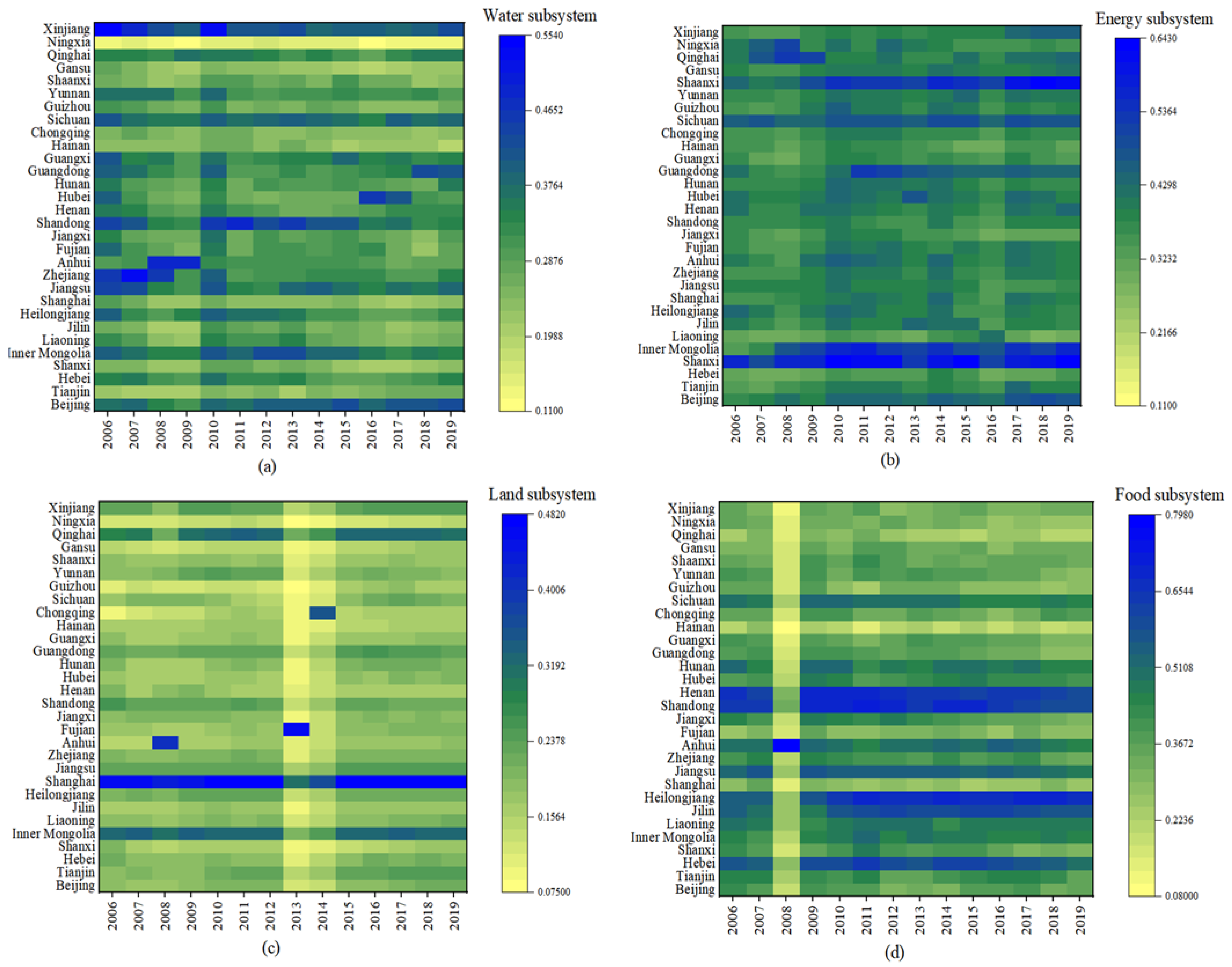
3.1. Analysis of Comprehensive Evaluation Index of WELF Nexus

According to the evaluation index system, the entropy method was used to calculate the weight of each evaluation index in each subsystem of water, energy, land and food from 2006 to 2019. In the water subsystem, water consumption per capita (W5) and urban sewage discharge (W11) were given lower weights. In the energy subsystem, total CO₂ emission (E12) had the lowest weight. In the land subsystem, the indicator weights were ranked as follows: land area occupied per capita (L1) > GDP per land (L13) > wetland area ratio (L8) > forestry land area (L6) > rate of forest cover (L9) > forestation area (L12) > area of built-up (L3) > greening coverage of built-up areas (L5) > arable land area ratio (L7) > agricultural land conversion (L10) > urban road area per capita (L4) > relief amplitude (L2) > sanded land area (L11). In the food subsystem, the contribution of agricultural machinery power (F3) was the lowest. Further, the weights of water resources per capita (W1), total energy generation (E1), land area occupied per capita (L1), and total crop area sown (F1) were always at high levels. These indicators are the factors that contributed the most to the water, energy, land, and food subsystems, respectively. The reason is that resources provide products and service functions, which are the natural conditions for human survival. As resources can constrain China’s economic growth [98], the importance of total resources is self-evident. However, resources are non-exclusive and finite, leading to increasing scarcity in the face of growing demand for resources. The shortage of resources is a bottleneck to comprehensive and sustainable development, which restricts human productive activities, and the rational exploitation of natural resources has become particularly urgent.

Figure 1 depicts the comprehensive evaluation indices of water, energy, land and food subsystems in 30 provinces of China from 2006 to 2019. In the water resources subsystem, the high scores were mostly clustered in the eastern coastal areas. Although the per capita water resources in Shandong were not the highest, the annual water-saving irrigation area was 2628.95 thousand hm², and the annual urban water saving consumption was 642.12 million m³, which resulted in a relatively high comprehensive evaluation index for Shandong’s water resources system. The evaluation index of water resources in Ningxia was relatively low, mainly due to the low precipitation, lack of water resources, and low proportion of domestic water, among which the annual precipitation was only 15.861 billion m³. Inner Mongolia, Shanxi and Shaanxi received high scores for their energy subsystems; this was mainly due to their good energy resource reserves, such as coal, and their high energy self-sufficiency rates. Annual total energy production in Shanxi reached 647.58 million tons of standard coal, about 300 times higher than that of Hainan. In the land subsystem index, Shanghai and Inner Mongolia scored higher. Although Shanghai has relatively low per capita land area, and its land resources are in short supply, its land use structure is relatively reasonable; the ratio of wetland area was as high as 73.27% in 2013, and Shanghai has always led the country in average land GDP. Benefiting from the advantages of vast land resources and sparse population, Inner Mongolia’s comprehensive land evaluation index has also been in the forefront. In the grain subsystem, the comprehensive evaluation index for Shandong, Henan and Heilongjiang is more outstanding. Shandong, Henan and Heilongjiang are the major grain producing provinces in China, with average annual grain yield per unit area of 6.20 t/hm², 5.73 t/hm² and 4.69 t/hm², respectively. Moreover, with the advantages of flat terrain, the level of agricultural machinery power has also been an important factor promoting the high yield of grain in these areas. However, Hainan is in a special geographical location, with less cultivated land area, an average annual grain sown/area proportion of 47.31%, and a low grain self-sufficiency rate. The grain problem in Hainan has long been a prominent challenge that needs to be solved.

3.2. Spatial-Temporal Characteristics of the Coupling Coordination of the WELF Nexus

3.2.1. Time-Series Change Characteristics

Based on the comprehensive evaluation index system, the entropy weight method was used to measure the coupling coordination degree of the WELF nexus in 30 provinces, and the results for 2006, 2010, 2014 and 2019 are shown in

Table 3. Level of coupling and coordination of the WELF nexus in 30 provinces.

Province	2006	2010	2014	2019	Average
Beijing	0.5672	0.5792	0.5469	0.5930	0.5668
Tianjin	0.5322	0.5519	0.5358	0.5524	0.5414
Hebei	0.5817	0.5905	0.5626	0.5775	0.5678
Shanxi	0.5783	0.5707	0.5363	0.5464	0.5427
Inner Mongolia	0.6081	0.6634	0.6308	0.6429	0.6311
Liaoning	0.5620	0.5711	0.5311	0.5442	0.5419
Jilin	0.5598	0.5835	0.5482	0.5589	0.5522
Heilongjiang	0.6099	0.6342	0.5931	0.6020	0.5980
Shanghai	0.5874	0.5903	0.5678	0.5734	0.5687
Jiangsu	0.6187	0.6176	0.6004	0.5985	0.5977
Zhejiang	0.5830	0.5850	0.5537	0.5555	0.5598
Anhui	0.5507	0.5751	0.5589	0.5573	0.5725
Fujian	0.5340	0.5437	0.5120	0.5310	0.5307
Jiangxi	0.5645	0.5844	0.5232	0.5218	0.5366
Shandong	0.6382	0.6422	0.6169	0.6026	0.6139
Henan	0.6134	0.6056	0.5559	0.5879	0.5763
Hubei	0.5681	0.5677	0.5391	0.5572	0.5512
Hunan	0.5861	0.5900	0.5574	0.5755	0.5589
Guangdong	0.5892	0.5908	0.5554	0.5760	0.5693
Guangxi	0.5700	0.5567	0.5338	0.5318	0.5361
Hainan	0.4840	0.4946	0.4489	0.4619	0.4704
Chongqing	0.4905	0.5364	0.5757	0.5198	0.5121
Sichuan	0.5997	0.6106	0.5678	0.5980	0.5889
Guizhou	0.5054	0.5168	0.5064	0.5097	0.5020
Yunnan	0.5663	0.5785	0.5445	0.5345	0.5532
Shaanxi	0.5485	0.5653	0.5364	0.5514	0.5461
Gansu	0.5197	0.5149	0.4903	0.5211	0.5023
Qinghai	0.5597	0.5772	0.5401	0.5685	0.5633
Ningxia	0.4688	0.4815	0.4508	0.4520	0.4585
Xinjiang	0.5962	0.6008	0.5503	0.5946	0.5702

. During the sample period, the average value of the coupling coordination degree of the WELF nexus in each region was 0.47~0.64, mostly at the stage of reluctant coordination, which shows that the promotion effect of water, energy, food and land was about equal to the inhibition effect, and had not yet entered the ideal coupling coordination state. On the whole, the coupling coordination degree showed an “N” type evolutionary pattern of rising, then falling and then rising during the sample observation period, and the coupling coordination development of the WELF nexus in each region was not stable. With the promotion of the ecological civilization in China, the sustainable use of resources has achieved initial results, and the South-North Water Diversion Project has helped to adjust the uneven spatial distribution of water resources, which in turn has improved the coordination of regional resources. However, the rigid demand for resources due to population growth and economic development is still huge, and there are still fluctuations in the coupled and coordinated development of the WELF nexus. In a few regions, the coupling coordination degree of the WELF nexus has shown a slight increase and a tendency to stabilize, and has risen more quickly in Chongqing, from 0.4905 in 2006 to 0.5198 in 2019, with a growth rate of 5.97%. However, most regions have shown declining characteristics; for example, Shanxi, Jiangxi, Shandong, Guangxi, and Yunnan all have growth rates of −5.5% or more. The reason for this may be that the economic scale of these regions is increasing, and their economic development has been relatively disorderly, such that demand for fossil energy and water resources is still increasing, and the pressure on resources is prominent [99], which affects the synergistic development of the WELF nexus.

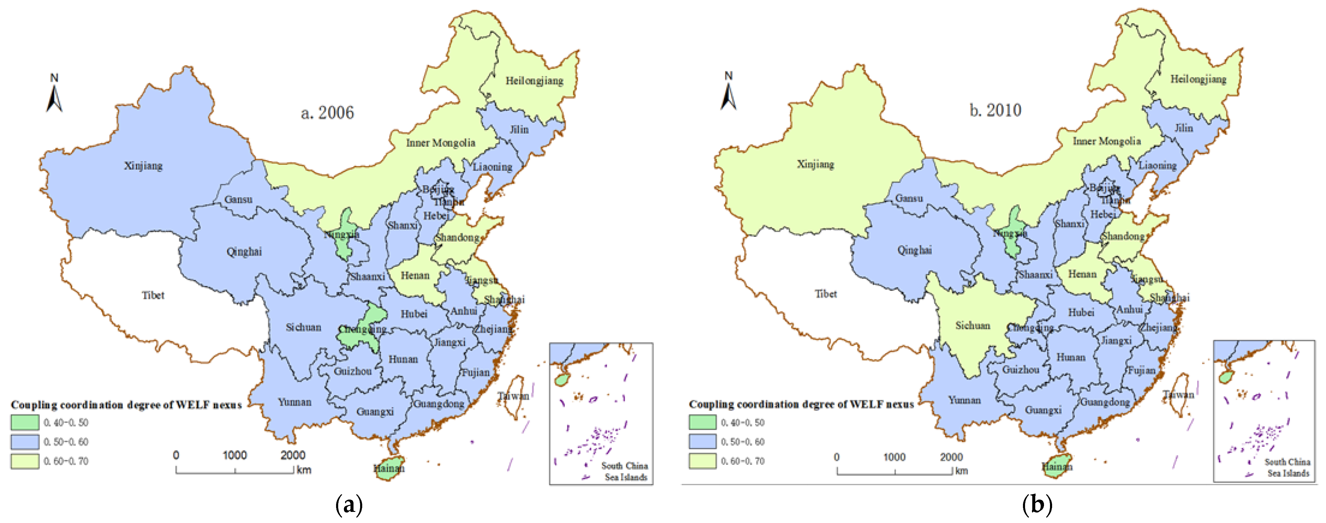
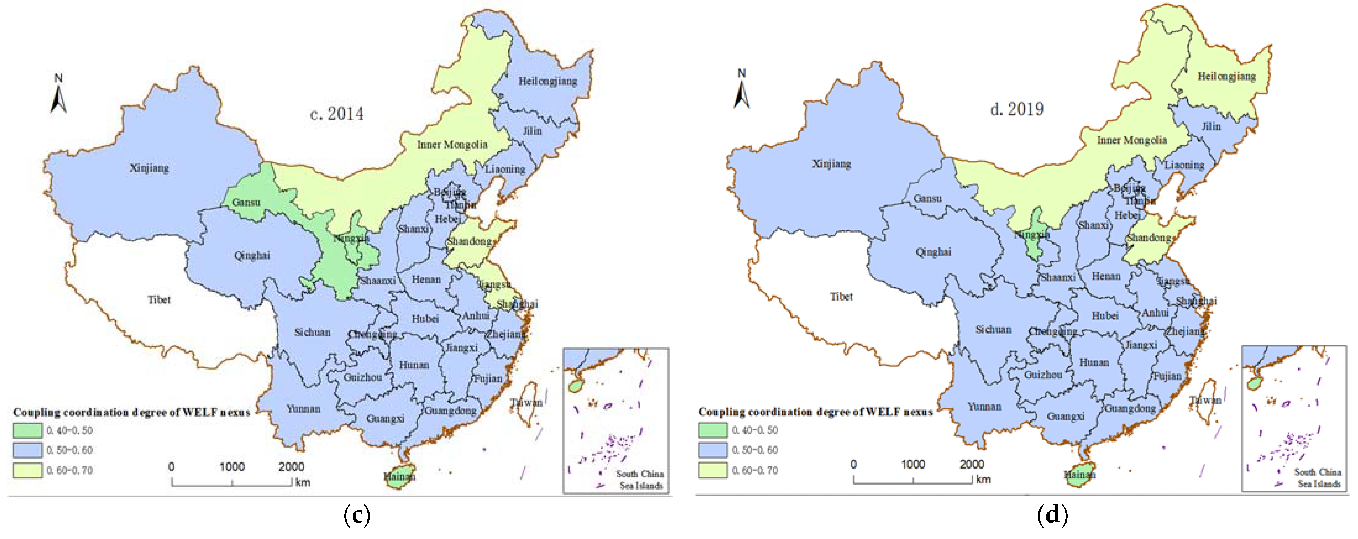
3.2.2. Spatial Distribution Characteristics

In order to reflect more intuitively the characteristics of spatial variation in the degree of coupling and coordination of the WELF nexus in China, ArcGIS 10.2 was used to visualize the coupling coordination degree of the WELF nexus in 2006, 2010, 2014 and 2019. The results of spatial distribution are shown in Figure 2. As a whole, the WELF nexus in most provinces remains barely coordinated. At the same time, the coupling coordination degree of the WELF nexus presents regional heterogeneity. Most provinces with poor coupling coordination are concentrated in the western region. Ningxia has faced the risk of near-disorder for a long time, and Chongqing and Gansu are facing a transition from barely coordinated to near-disorder. The industrial and economic foundations of Inner Mongolia are weak, focused mainly in the development of primary industry, but because its reserves of natural resources are good, the coupling coordination degree of its WELF nexus has maintained a primary coordination status for a long time. The development of the four subsystems of water, energy, land and food in Hunan and Hubei in the central region is barely balanced, and the positive effects among the four subsystems are approximately equal to the negative effects. The coupling coordination degree of Henan has gradually devolved from primary coordination to barely coordinated, probably because of its flat topography and its early role as the main grain producing area in China; however, with the intensification of water shortages and “heavy” industrial structure, the coordinated development of its WELF nexus has been less effective. The overall coupling coordination in the eastern region is high; most provinces are barely coordinated, while only Hainan has been in a state of near-disorder for a long time. The primary coordination is concentrated in Shandong and Jiangsu; they are promoting sustainable and healthy economic development, and the coupling coordination of the WELF nexus has also been a focus of their attention to promote coordinated economic development and ecological protection.

Review No. GS (2019) 1822 (supervised by the Ministry of Natural Resources), with no modification of the base map (excluding data from Tibet, Hong Kong, Macao and Taiwan)

3.3. Analysis of Regional Differences and Their Decomposition in the Coupling Coordination of the WELF Nexus

The Dagum Gini coefficient method was used to measure the regional differences in the coupled coordination of WELF nexus and their sources of contribution in the whole country and the three regions of east, central and west. The results are shown in

Table 4. National and intra-regional Gini coefficients.

Year	National		Intra-Regional Gini Coefficients
		East	Middle	West
2006	0.0394	0.0391	0.0206	0.0459
2007	0.0373	0.0388	0.0161	0.0428
2008	0.0499	0.0381	0.0541	0.0475
2009	0.0410	0.0347	0.0276	0.0522
2010	0.0377	0.0343	0.0182	0.0483
2011	0.0411	0.0389	0.0232	0.0514
2012	0.0344	0.0319	0.0193	0.0417
2013	0.0407	0.0402	0.0208	0.0468
2014	0.0380	0.0412	0.0189	0.0450
2015	0.0367	0.0349	0.0153	0.0485
2016	0.0396	0.0332	0.0205	0.0531
2017	0.0384	0.0320	0.0251	0.0497
2018	0.0393	0.0349	0.0236	0.0499
2019	0.0394	0.0351	0.0229	0.0497

and

Table 5. National and intra-regional Gini coefficients.

Year	Inter-Regional Differences			Variance in Contribution Rate (%)
	East—Middle	East—West	Middle-West	Intra-Regional	Inter-Regional	Hypervariable Density
2006	0.0320	0.0462	0.0405	32.5112	30.3715	37.1173
2007	0.0328	0.0440	0.0356	32.4489	23.0123	44.5387
2008	0.0503	0.0481	0.0601	30.6870	32.6326	36.6804
2009	0.0335	0.0456	0.0438	33.1863	14.1369	52.6768
2010	0.0281	0.0444	0.0408	32.6500	24.9665	42.3835
2011	0.0323	0.0475	0.0421	33.4238	16.8178	49.7584
2012	0.0268	0.0401	0.0365	32.6211	22.1026	45.2762
2013	0.0337	0.0497	0.0388	32.3035	26.7726	40.9239
2014	0.0317	0.0446	0.0353	33.9297	13.6805	52.3898
2015	0.0266	0.0445	0.0373	33.3829	18.2844	48.3326
2016	0.0279	0.0476	0.0429	32.7557	22.0087	45.2356
2017	0.0294	0.0442	0.0411	33.1568	15.2031	51.6401
2018	0.0311	0.0457	0.0405	33.1482	13.6465	53.2054
2019	0.0302	0.0464	0.0414	32.8915	16.1355	50.9730

.

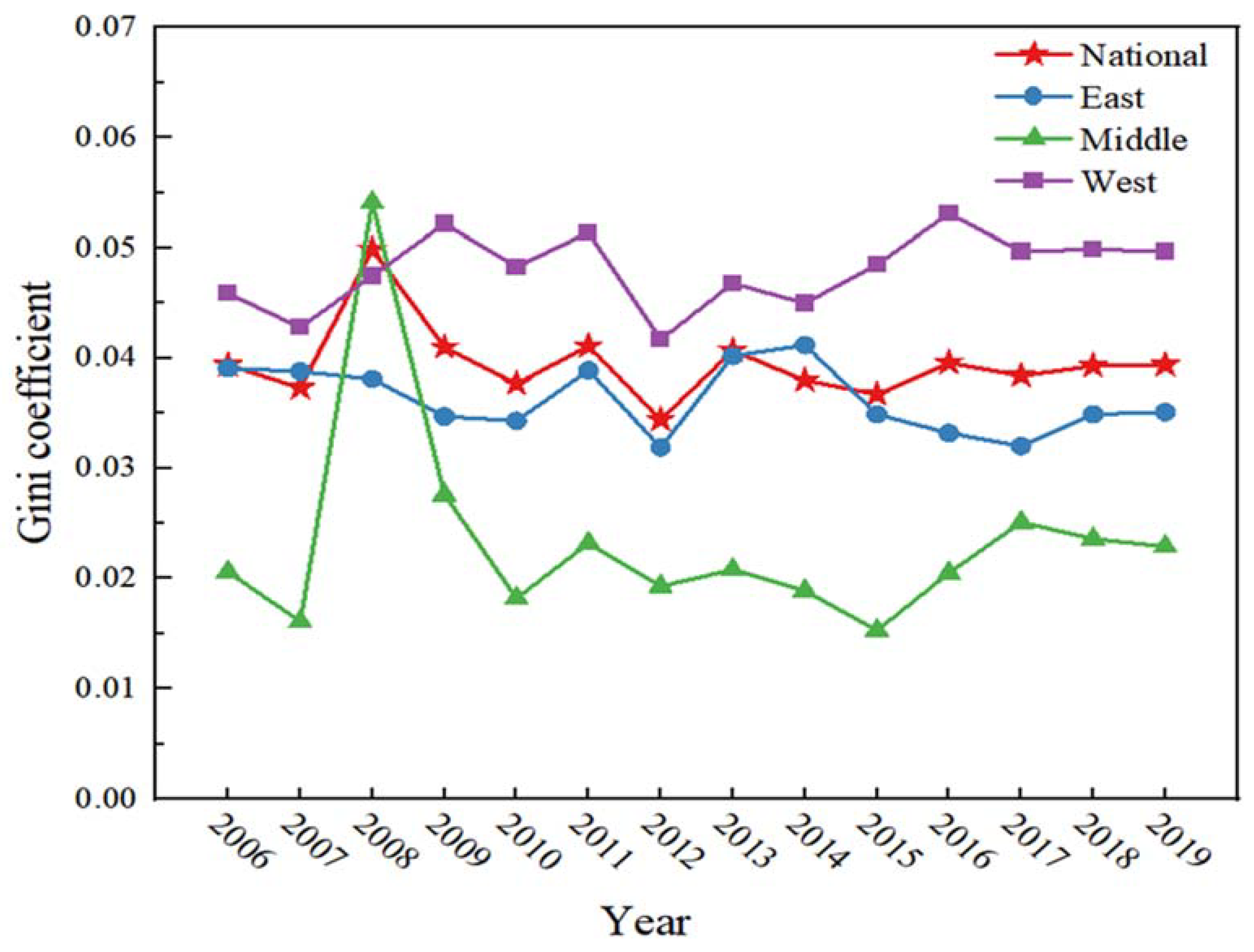
3.3.1. National and Intra-Regional Differences

Figure 3 shows the Gini coefficient and characteristics of change in the coupling coordination degree of the WELF nexus for the whole country and the three considered regions. From a national perspective, the overall variation in the coupling coordination degree of the WELF nexus from 2006 to 2019 was small, with the Gini coefficient ranging from 0.0344 to 0.0499, reaching a maximum value of 0.0499 in 2008, followed by a small decline from 2010 to 2011, and then an uneven rise in 2011. It then fell to a minimum value of 0.0344 in 2012 and showed a slight upward trend in 2013, after which it maintained a steady trend in general until 2019, fluctuating slightly above and below 0.039. This shows that there was a relatively small difference between the provincial levels of coordination of the WELF nexus nationwide, but the overall trend was clearly fluctuating and generally unstable.

The Gini coefficients of the coupled WELF nexus in the eastern, central and western regions vary. Specifically, the Gini coefficient in the eastern region can be broadly classified as “steadily declining”, “steeply rising”, “fluctuating declining”, “slowly rising”, “steadily increasing”, and “stabilizing and rising “. That is, 2006 to 2010 showed a steady downward trend, followed by a steep upward momentum in 2011, a fluctuating downward trend in 2012, a slow upward trend in 2012 to 2014, a flat downward trend thereafter that continued until 2017, and an upward trend in steady state fluctuations from 2017 to 2019. During the sample observation period, the overall Gini coefficient in the east decreased slightly, by nearly 0.004, or about 10.23%. The Gini coefficient in the central region fluctuated more sharply, and the evolutionary trend was as follows: a decreasing trend from 2006 to 2007, followed by a sharp increase in 2008, reaching a maximum value of 0.0541 during the observation period, then a sharp decreasing trend from 2008 to 2010, a fluctuating rebound in 2011, then a small decreasing trend lasting until 2015, followed by a growth trend from 2015 to 2017, and then a steady decreasing trend. During this period, the Gini coefficient in the central region increased by nearly 0.0023 compared with 2006, for an increase of about 11.17%. The evolutionary trend in the western region was marked by irregular fluctuation, with a downward trend in 2007 and an overall “M” shaped trend from 2007 to 2012, i.e., it was an upward phase from 2007 to 2009, then showed a fluctuating downward trend from 2009 to 2010, followed by a rebound phase from 2010 to 2011 and a sharp downward trend from 2011 to 2012. The overall trend was steadily increasing from 2012 to 2016, followed by a stabilization and decline phase through 2019. During the observation period, the Gini coefficient for the western region also increased, rising by nearly 0.0038, or about 8.28%.

In 2008, the Gini coefficient for the whole country and the central region fluctuated significantly. The reason may be that the global food crisis in 2008 affected the production of and income from Chinese food, and the reduction in cultivated land area and the quality of cultivated land also affected the development of food. These influences caused abnormal changes in the grain subsystems in Heilongjiang, Shandong and other provinces with large-scale grain production, which led to a significant decline in the coupling coordination degree. However, the fluctuation in the coupling coordination degree in most provinces was relatively smooth, and the comprehensive evaluation index of the grain subsystem in Anhui remained at a high level; together, these factors aggravated the differences between the whole country and the central region. On the whole, the coupling coordination degree of the WELF nexus in the eastern region showed a small decline, while the central and western regions showed weak growth trends amidst fluctuations. Comparing the values, we can see that the Gini coefficient in the western region was larger than that in the eastern and central regions, and the average values of the three regions were 0.0480, 0.0362 and 0.0233, respectively, which meant that the unbalanced development of the coupled WELF nexus in the western region was the most prominent, followed by the eastern region and finally the central region. Possible reasons for this phenomenon were the high degree of coordination of the WELF nexus coupling in Sichuan, and the low levels of water, energy and food adaptability in the western provinces of Gansu and Ningxia. In addition, water resources were abundant in the southwest and scarce in the northwest, and there were differences in the stability of the water systems, which aggravated the unevenness of the coupling coordination of the WELF nexus in the western provinces.

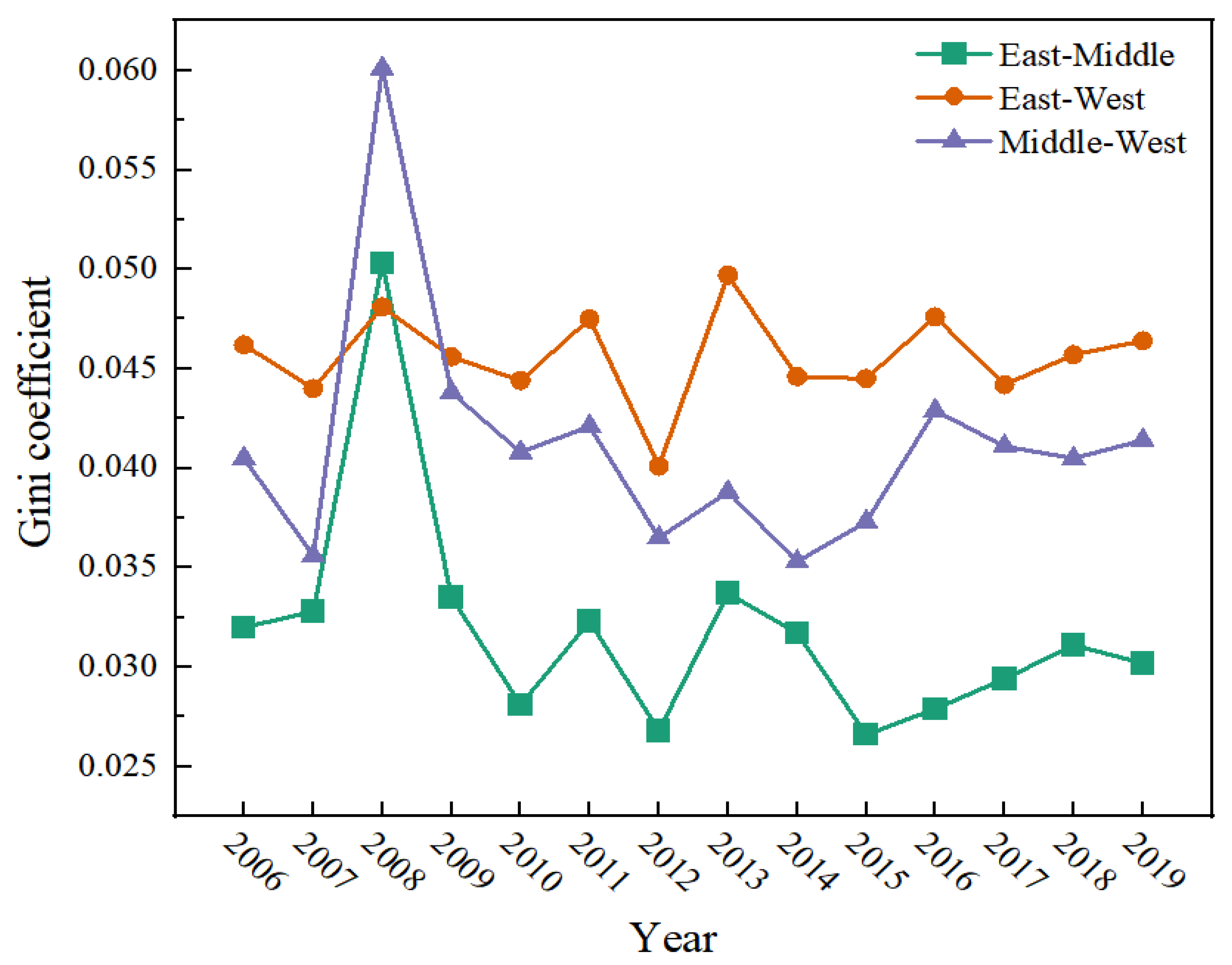
3.3.2. Inter-Regional Differences

Figure 4 depicts the evolution of the inter-regional differences in the coupling coordination degree of the WELF nexus during the observation period. Among them, the east-central region roughly went through a process of “rapid increase—sharp decrease—small increase—steep decrease—fluctuating rebound—obvious decrease—steady increase—slight decrease”, with a rapid increase from 2006 to 2008, a sharp decrease from 2008 to 2010, followed by a small increase in 2011, a decline in 2012, and a fluctuating rebound in 2013. The sharp rise was followed by a sharp decline from 2008 to 2010, then by a slight rise in 2011, a decline in 2012, a fluctuating rebound in 2013, a significant decline from 2013 to 2015, and a steady rise from then to 2018. Overall, the east-middle interregional Gini coefficient declined from 0.0320 in 2006 to 0.0302 in 2019, a decrease of nearly 0.0018, or about 5.63%. The overall fluctuation in the Gini coefficient between the eastern and western regions was relatively small, as follows: a small decline from 2006 to 2007, an upward trend in 2008, a steady declining trend from 2008 to 2010, a fluctuating rebound in 2011, followed by a steep decline to a minimum value of 0.0401 in 2012, a sharp increase in 2013, a decline from 2013 to 2015, a rebound and rise in 2016, and a downward trend in 2017, followed by a more moderate growth trend in 2018–2019. The change in the Gini coefficient between the East-West regions was small, and even though there were several upward trends, it did not have a large impact on the overall flat declining trend. The Gini coefficient between the central and western regions could be roughly divided into “steep decline—sharp rise—rapid decline—steady rise—gentle decline” phases, i.e., it showed a steep decline from 2006 to 2007, reached a maximum in 2008 during the observation period, showed a sharp decline from 2008 to 2014, although fluctuating and rising in 2011 and 2013, but still maintained a declining trend overall, and then showed a steady rise until 2016, followed by a gentle decline from 2016 to 2019. During the observation period, the Middle-West Gini coefficient increased from 0.0405 in 2006 to 0.0414 in 2019, an increase of nearly 0.0009, or only 2.22%.

During the observation period, the inter-regional differences between the eastern and middle regions showed a slight decrease, while the overall differences between eastern and western regions did not change significantly, and the differences between middle and western regions showed a slight increase. In terms of magnitude, of the inter-regional Gini coefficient, the inter-regional differences in the coupling coordination of the WELF nexus during the observation period were as follows, in descending order: East-West, Middle-West and East-Middle, with mean values of 0.0456, 0.0412 and 0.0319, respectively. Most of the eastern regions are economically developed coastal provinces with abundant water resources, sufficient energy resources and reasonable land use planning, and most of the provinces have good WELF nexus coordinated development capacity. The northwest region suffers from water and food scarcity and poor land quality, and its energy resources cannot easily make up for these disadvantages in water, land and food. In addition, with the increase in coal and oil mining in the western development strategy, energy use has been growing, and accelerated urbanization in the western region in recent years has further aggravated the imbalance between water, energy, food and land. Regional differences in economic development and resource abundance have led to significant differences in the coupling coordinated development of the WELF nexus between the eastern and western regions.

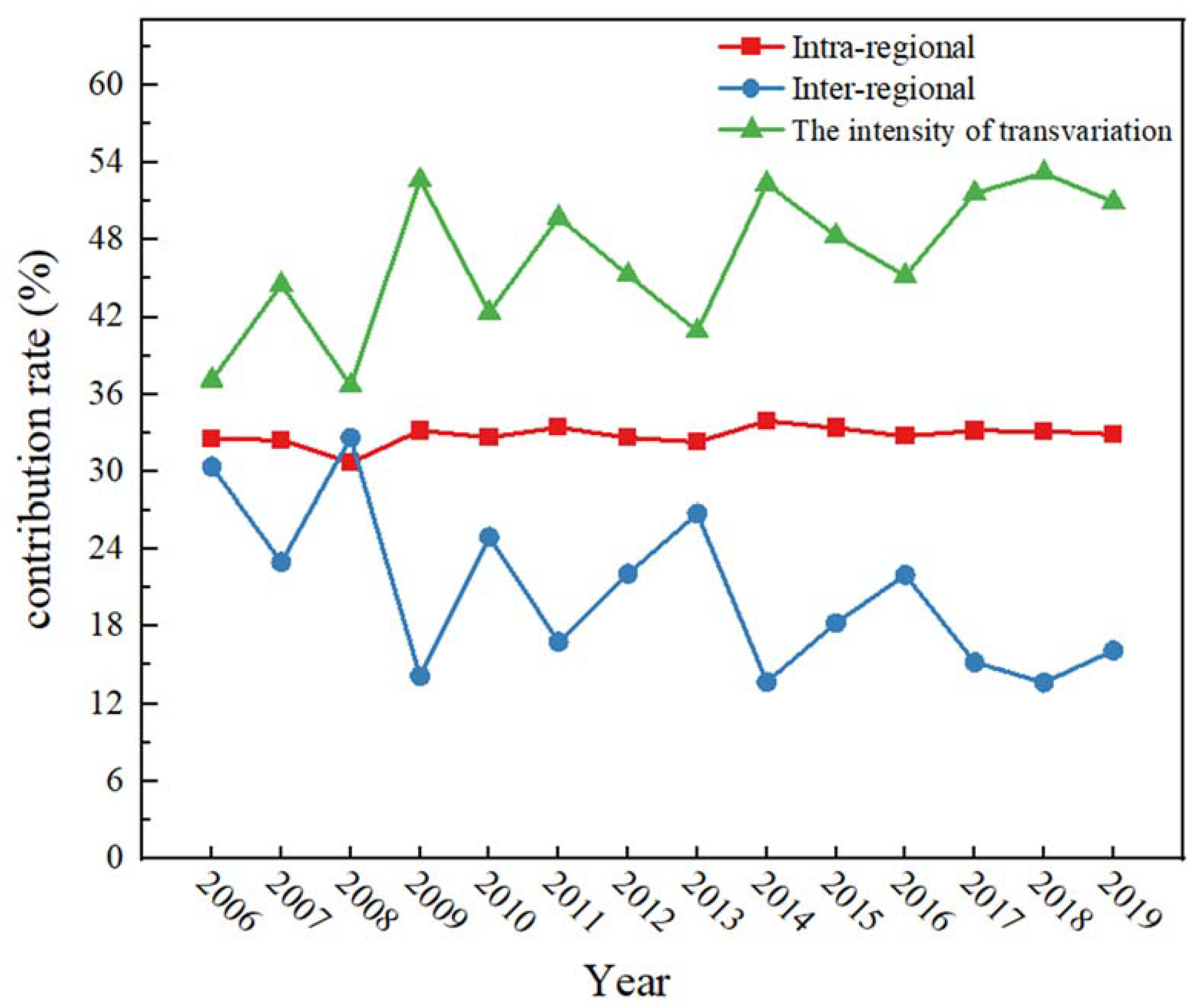
3.3.3. Sources of Variation and Contribution Rates

Figure 5 depicts the evolution of the sources of variation in the coupling coordination of the WELF nexus. It can be seen that the intra-regional contribution rate was 32.51% in 2006, and then remained basically stable as a whole. During the sample observation period, the intra-regional contribution rate fluctuated around 32.5%, with a small decrease reaching a minimum value of 30.69% in 2008, but that did not have a large impact on the overall stable trend. The intra-regional contribution rate reached 32.89% in 2019; compared with 2006, that was down by 0.38%, for a decrease of about 1.17%. The inter-regional contribution rate showed a declining trend with fluctuations, reaching 30.37% in 2006 and then roughly going through a process of “small decline—rebound upward—substantial decline—fluctuating upward—obvious decline—steady growth—sharp decline—counter trend upward—slowing tend”. The inter-regional contribution rate in 2019 reached 16.14%, down significantly, by 14.23%, compared to 2006, for an overall decline of about 46.86% and an average annual 3.60% rate of decline, during the observation period. The intensity of transvariation effectively reflected the contribution rate of the overlap between different regions to the overall region, and the contribution rate during the sample observation period irregularly fluctuated upward, to 37.12% in 2006 and 50.97% in 2019, an increase of nearly 13.85%, or about 37.31% compared to 2006, with an average annual growth rate of 2.87%.

In terms of the magnitude of the contribution rate, the intensity of transvariation was the main source of regional differences in the coupling coordination of the WELF nexus in China during the sample observation period, followed by intra-regional differences. The contribution of intra-regional variation was relatively flat overall, and the contribution of inter-regional variation was significantly lower. The mean contributions of the three variables were 46.51%, 32.79%, and 20.70%, respectively. It can be seen that the main source of regional difference in the coupled coordination of the WELF nexus from 2006 to 2019 was the intensity of transvariation, followed by intra-regional variation, while the contribution from inter-regional variation was relatively small.

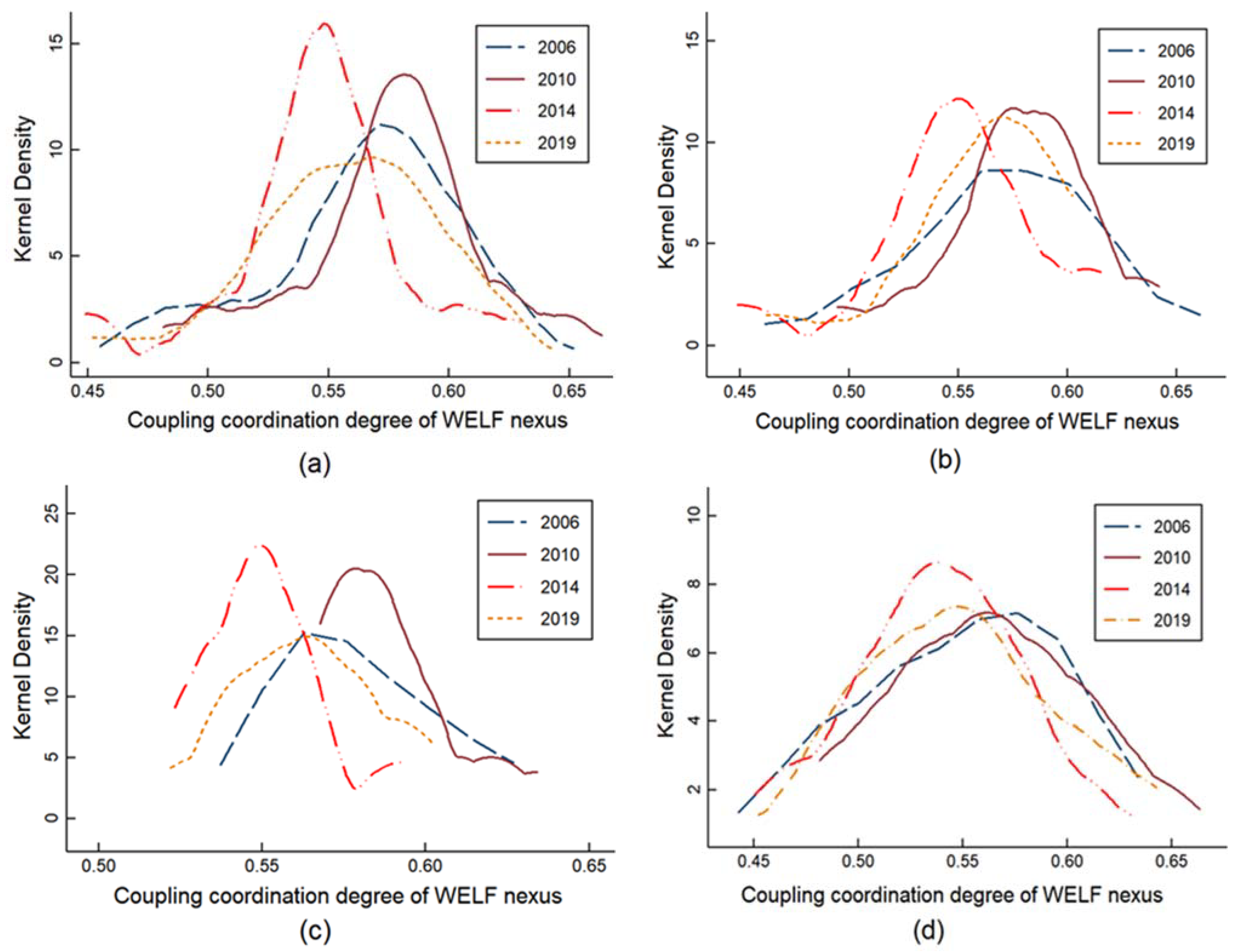
3.4. Dynamic Evolution of Nuclear Density Distribution

In this paper, the kernel density estimation method was applied to characterize the distribution dynamics of in the whole country and the three regions in terms of location, dynamics, extension and polarization trends, revealing information on the dynamics of the coupled WELF nexus coordination. The kernel density estimation results are shown in Figure 6.

From the viewpoint of distribution position, the middle line of the distribution curve for the whole country and the three regions shows a small leftward trend, and the specific pattern of change was: first rightward—then leftward—then rightward, which indicates that the coupling coordination degree of the WELF nexus for the whole country and the eastern, central and western parts of the country were generally in a rising-decreasing-rising trend, but decreasing in general.

In terms of the distribution pattern, the trend of change was almost the same for the whole country and the three regions. The distribution curves for the sample period show that the height of the main peak was evolving through a pattern of “steadily increasing—slightly decreasing”, and the width of the main peak was evolving through a pattern of “slightly narrowing—significantly widening”, which means that the differences between the whole country and the three regions were also going through a pattern of “smaller—larger”. However, in 2019 relative to 2016, the national differences were slightly widening, the trend in the eastern region was narrowing overall, and the trends in the central and western regions were, overall, relatively less obvious.

From the viewpoint of distribution extension, the national, eastern and middle regions gradually displayed an obvious right-trailing phenomenon, while the western region did not. This meant that the provinces with high coupling coordination of the WELF nexus in the national, eastern and central regions maintained strong improvements, and a gap was formed with provinces with low coupling coordination. The difference between provinces with high coupling coordination and provinces with low coupling coordination in the western region was slightly reduced.

In terms of polarization, the nation and three regions had different performance. The country gradually evolved from a “single peak” state to a “main side” bimodal state, and then returned to a “single peak” and a bimodal state. The eastern region had a single-peaked state in general, and in 2010, it had a main peak and a slightly smaller side peak. The central region mainly experienced the evolution of single peak to “one main and one side” double peak. The bimodal phenomenon was not obvious in the western region. This indicates that the national, eastern and central regions had a slight gradient effect, and regional dispersion in the coupling coordination of the WELF occurred but was less obvious.

3.5. Spatial Convergence Analysis of WELF Nexus Coupling Coordination

3.5.1. Source of Variation and Contribution Rate

Based on the geographical coordinates of each province, an inverse distance spatial weight matrix was constructed, and then the global spatial correlation of the coupling coordination degree of the WELF nexus was tested. The results listed in

Table 6. Global Moran’s I of the coupling coordination of the WELF nexus.

Year	Moran’s I	E(I)	Sd(I)	Z	p-Value
2006	0.000	−0.034	0.033	1.051	0.147
2007	0.013	−0.034	0.034	1.421	0.078
2008	0.035	−0.034	0.030	2.336	0.010
2009	−0.015	−0.034	0.033	0.574	0.283
2010	0.013	−0.034	0.033	1.454	0.073
2011	0.037	−0.034	0.033	2.182	0.015
2012	0.026	−0.034	0.033	1.849	0.032
2013	0.023	−0.034	0.033	1.748	0.040
2014	0.012	−0.034	0.032	1.445	0.074
2015	0.015	−0.034	0.032	1.540	0.062
2016	0.019	−0.034	0.033	1.649	0.050
2017	0.003	−0.034	0.033	1.150	0.125
2018	0.026	−0.034	0.033	1.830	0.034
2019	0.024	−0.034	0.033	1.785	0.037

show that the global Moran’s I index distribution was positive except for 2009, and that all values passed the significance test in general. This indicates that the coordination degree of WELF nexus coupling was spatially positively correlated from 2006 to 2019, with a high–high and low–low spatial clustering phenomenon. The Moran’s I index showed irregular fluctuations, generally increasing from 2006 to 2011 and reaching a maximum value of 0.037 in 2011, highlighting the aggregation trend. From 2011 to 2014, the Moran’s I index decreased significantly, and after 2014, it fluctuated and leveled off. The spatial distribution degree of WELF nexus coupling coordination in China is relatively unstable, and also shows a certain spatial aggregation effect. This is because provinces with a high degree of coupling coordination radiate and drive neighboring provinces by means of linkage cooperation and technology spillover, forming high–high aggregation regions of benign and coordinated development. While the coordinated development of the WELF nexus is influenced by resource endowment and geographical location, provinces with a low degree of coupling and coordination have poor capacity for coordinated development of water, energy, land and food, and neighboring regions also face the same problems, with little cooperation between the two sides, making it difficult to break through regional restrictions and forming a low–low aggregation dilemma.

3.5.2. Spatial Absolute β Convergence Analysis

The spatial absolute β convergence process of the coupled coordination degree of the WELF nexus was analyzed by using the spatial lag model (SAR) based on the results of the LM test, Hausman test, fixed effect test, Wald test and LR test. Fixed effects were selected when the Hausman test value was negative [100]. According to the results in

Table 7. Spatial absolute β-convergence of the coupling coordination of WELF nexus.

Region	National	East	Middle	West
Model Type	Time-space double fixed effects SAR model	Time-space double fixed effects SAR model	Time-space double fixed effects SAR model	Time-space double fixed effects SAR model
$\beta$	−0.5334 ***(0.0422)	−0.5066 ***(0.0675)	−0.7130 ***(0.0905)	−0.4554 ***(0.0613)
$\rho$	0.6869 ***(0.0384)	0.6284 ***(0.0533)	0.3757 ***(0.0922)	0.6997 ***(0.0456)
$R^2$	0.2773	0.2817	0.3124	0.3246
N	390	143	104	143
$\eta$	0.0586	0.0543	0.0960	0.0467

Note: *** denote significance at the 10%, 5%, and 1% levels, respectively; t-statistic in parentheses; and η is the rate of convergence (η = −ln(1 + β)/T).

, the spatial lag coefficient ρ was significantly negative, and the spatial absolute β convergence coefficients of the coupling coordination degree of the WELF nexus in the national, eastern, central and western regions were all negative, and they all passed the 1% significance test, indicating that the spatial absolute β convergence process existed for the coupling coordination degree of the WELF nexus in the whole country and the three regions. This means that in provinces with similar population density, economic development level and other factors, the coupling coordination degree of the WELF nexus in each province eventually trends toward a similar steady state level, and the provinces with a lower coupling coordination degree have higher coupling coordination growth rates than those with a higher coupling coordination degree. The differences in WELF nexus coupling coordination degree showed a gradually decreasing trend. Among them, the national convergence rate was about 5.86%, whereas the central region had the fastest convergence rate, followed by the eastern region, and the western region was the slowest, with convergence rates of 9.60%, 5.43%, and 4.67%, respectively. This indicates that a series of environmental protection policies such as ecological civilization construction and ecological synergistic governance in the context of the new era in China have achieved remarkable results, and the factors are in deep coupling and synergistic symbiosis to promote high-quality economic development.

3.5.3. Spatial Condition β Convergence Analysis

In fact, there is heterogeneity in the development status of different regions, so this paper used spatial conditional β convergence analysis to further consider the influence of control variables, and selected spatial econometric models that satisfy the test rules for different regions. The selected model types and spatial conditional β convergence results are shown in

Table 8. Spatial absolute β-convergence of the coupling coordination of the WELF nexus.

Region	National	East	Middle	West
Model Type	Time-space double fixed effects SDM model	Time-space double fixed effects SAR model	Time-space double fixed effects SEM model	Time-space double fixed effects SAR model
$\beta$	−0.8423 *** (0.0451)	−0.9693 *** (0.0839)	−0.7116 *** (0.0474)	−0.5037 *** (0.0641)
$\rho$	0.7546 *** (0.0481)	0.6489 *** (0.0637)		0.6823 *** (0.0465)
$\lambda$			−0.7546 *** (0.2346)
Popu	−0.0139 *** (0.0018)	−0.0026 (0.0029)	−0.0469 *** (0.0027)	−0.0195 (0.0276)
Pgdp	0.0085 *** (0.0021)	0.0036 (0.0027)	0.0171 * (0.0091)	−0.0014 (0.0039)
Urba	−0.0023 *** (0.0005)	−0.0003 (0.0010)	0.0014 ** (0.0006)	0.0002 (0.0007)
Indu	0.0305 (0.0299)	−0.0293 (0.0573)	−0.0543 (0.0480)	0.0453 (0.0420)
Envi	0.0001 (0.0001)	0.0013 (0.0017)	0.0027 (0.0021)	0.0001 (0.0001)
Weat	−0.0085 *** (0.0029)	−0.0021 (0.0054)	−0.0061 ** (0.0028)	−0.0068 ** (0.0033)
Huma	−0.0078 (0.0050)	−0.0009 (0.0084)	−0.0012 (0.0090)	0.0054 (0.0071)
$R^2$	0.0323	0.1213	0.0460	0.1239
N	390	143	104	143
$\eta$	0.1421	0.2680	0.0956	0.0539

Note: *, **, *** indicate significance at the 10%, 5%, and 1% levels, respectively, with t-statistics in parentheses.

. From the results, it can be seen that the spatial conditional β convergence coefficients of the national, eastern, central and western regions were all negative, and all of them passed the 1% significance test. This indicates that a spatial β convergence process exists in the country and in each region under the influence of population density, urbanization level, economic development level, industrial structure, environmental protection input, climate, human capital factors and spatial spillover effects, and the coordination degrees of WELF nexus coupling in each province in a region gradually converge to their respective steady state levels over time. The national convergence rate is about 14.21%, while the convergence rates in the eastern, central and western regions are 26.80%, 9.56% and 5.39%, respectively. Compared with the spatial absolute β convergence results, factors such as population density, urbanization level, economic development level, industrial structure, environmental protection input, climate, and human capital speed up the convergence of the WELF nexus coupling coordination to some extent.

In terms of control variables, the magnitude and direction of the effect of each influencing factor on the coordination of the WELF nexus coupling varies from region to region. Population density has a significant negative impact on the coupling coordination degree of the WELF nexus in China and the central region, and restrains the convergence of the coupling coordination degree of the WELF nexus to a high level in the above regions. The greater the population density, the greater the demand for resources, and the contradiction between humans and land is further aggravated. Water, energy and food are also in short supply in the case of a large population. The level of economic development has a positive promoting effect on the coupling coordination degree of the WELF nexus in the whole country, the eastern region and the central region, and especially in the whole country and the central region, which is more significant, but the effect on the western region is negative and insignificant. The reason for this phenomenon may be that provinces with a high level of economic development have excellent financial, material and human resources that provide basic guarantees for the coordinated allocation of resources, but that also better promote the development and utilization of clean energy or alternative resources [101]. However, at present, the growth mode of the western region is mostly extensive, and the improvement in economic development level is at the cost of excessive consumption of resources, and the compatibility between resources is poor. Urbanization level has an opposite influence on the coupling coordination degree of the WELF nexus in the country and the central region, inhibiting the coordinated development of resources in the country, while promoting the convergence of the coupling coordination degree of the WELF nexus in the central region to a high level. In general, urban development occupies a large amount of cultivated land, and the impact on land use is unreasonable, which aggravates the imbalance of resources. However, rational urbanization in central China will develop green industries that consume less resources and optimize resource utilization. Temperature has a negative effect on the coupling coordination degree of the WELF nexus in China and the three studied regions, especially in terms of significantly inhibiting the convergence of the coupling coordination degree of the WELF nexus to a high level in China, central China and western China. The problem of global warming is becoming more and more serious, and droughts are frequent. Further increases in temperature will lead to water shortages and reduced grain production, which will aggravate the uneven distribution of water resources and hinder the coordinated development of resources. However, the impacts of industrial structure, environmental protection inputs and human capital on the coupling coordination degree of the WELF nexus are not the same, and they fail the significance test.

4. Conclusions and Recommendations

This study measured the coupling coordination level of the WELF nexus and analyzed its spatial and temporal distribution characteristics, regional differences and spatial convergence. We found that most of the 30 provinces in the country were at the stage of barely coordinated WELF nexus coupling coordination, and the overall level of coupling coordination in most provinces was decreasing. The primary coordination provinces were mostly gathered in the eastern region. Unevenness of coupling coordination is most prominent in the western region, and the difference between eastern and western regions was the most obvious. In terms of the contribution of regional differences, the intensity of transvariation was the main source of regional differences in the coupling coordination degree of the WELF nexus, followed by intra-regional differences, and the contribution of inter-regional differences was relatively small. Our findings also suggest that the provinces with high coupling coordination degrees of the WELF nexus at the national level and in the eastern and central regions maintained strong increases, forming gaps with provinces with low coupling coordination. The difference between provinces with high coupling coordination and provinces with low coupling coordination in the western region was slightly reduced. The national, eastern and central regions were marked by a slight gradient effect, and the coupling coordination degree of the WELF nexus showed the characteristics of regional dispersion but was less obvious. There was spatial absolute β convergence and spatial conditional β convergence in the coupling coordination degree of the WELF nexus for the whole country and the three regions.

Based on the above research findings, this paper puts forward several policy recommendations. First, allocate limited natural resources reasonably and promote the balanced development of the WELF nexus. Focusing on the shortage of natural resources, avoid overexploitation of natural resources [102], use renewable resources to replace or compensate for non-renewable or depleted resources, ease the consumption of resources and secure new resource reserves. Strengthen scientific and technological innovation to lead and accelerate key core technology research and development, promote the transformation and upgrading of industries with high water consumption, high energy consumption and low efficiency, accelerate the development of clean energy, improve comprehensive food production capacity, reasonably plan land use, and continuously improve the efficiency of water, energy, food and land production and use. At the same time, take into account the coordinated development of resources, break through factor bottlenecks, transform resource advantages into economic advantages, manage resources in a more scientific and comprehensive manner, and promote the coupled and coordinated development of the WELF nexus.

Second, strengthen regional resource linkages and sharing and optimize the spatial distribution pattern of resources. The unbalanced phenomenon of WELF nexus coupling and coordination is most prominent in the western region, and the difference between the eastern and western regions is greater than that between the central and western regions and the eastern and central regions. Given this phenomenon, it is necessary to strengthen top-level design, give full play to the regional synergy effect of policies, break through administrative barriers, establish cooperation mechanisms for resource utilization, strengthen the reasonable and appropriate cross-regional flow of resources, and enhance complementary advantages in resources between the eastern and western regions. For provinces with low levels of WELF nexus coupling and coordinated development, strengthen the policy orientation, especially in Ningxia and Hainan, which should focus on the application of resource-efficient methods and technologies. Provinces with high levels of WELF nexus coupling and coordinated development, such as Shandong, should serve as model high-level provinces to spread the benefits of nexus coupling and coordination. Therefore, promoting the flow and linkage of inter-regional factors and adhering to the national strategy are important steps to enhance the overall WELF nexus coupled and coordinated spatial correlation and gradually reduce the differences between regions.

Third, give full play to regional advantages and optimize the synergistic use of resources. The degree of WELF nexus coupling coordination is also affected by other factors. Based on the positive promotion of the level of economic development, optimize the investment of scientific research funds, promote technological innovation, and promote human, financial and material resources to adapt to the coupled and coordinated development of the WELF nexus. In promoting new urban development processes, protect the quantity and quality of arable land, adhere to the red line of arable land, and strictly adhere to the bottom line of resources. For provinces with high population density, it is more important to strengthen the cultivation of innovative talent, implement strategies to attract talent, promote human capital formation with an eye toward advanced development, and promote the transformation of the demographic dividend from quantity to quality. Continuously promote the reduction of carbon emissions, actively respond to climate change, and circumvent the impact of climate change on water security and food production. We should also consider the impact of multiple factors, optimize the sustainable and coordinated use of resources, improve the level of modernization of industry and agriculture, and promote coordinated, high-quality economic development and ecological protection.

References

1. Deng, F.; Li, H.; Yang, M.; Zhao, W.; Gai, Z.; Guo, Y.; Huang, J.; Hao, Y.; Wu, H. On the nonlinear relationship between energy consumption and economic and social development: Evidence from Henan province, China. Environ. Sci. Pollut. Res. 2021, 28, 33192–33207. [Google Scholar] [CrossRef] [PubMed]
2. Qian, X.; Liang, Q.; Liu, L.; Zhang, K.; Liu, Y. Key points for green management of water-energy-food in the belt and road initiative: Resource utilization efficiency, final demand behaviors and trade inequalities. J. Clean. Prod. 2022, 362, 132386. [Google Scholar] [CrossRef]
3. Du, D. The causal relationship between land urbanization quality and economic growth: Evidence from capital cities in China. Qual. Quant. 2017, 51, 2707–2723. [Google Scholar] [CrossRef]
4. Yu, B. Ecological effects of new-type urbanization in China. Renew. Sustain. Energy Rev. 2021, 135, 110239. [Google Scholar] [CrossRef]
5. Şimşek, H.; Öztürk, G. Evaluation of the Relationship between Environmental Accounting and Business Performance: The Case of Istanbul Province. Green Financ. 2021, 3, 46–58. [Google Scholar] [CrossRef]
6. Hao, Y.; Gao, S.; Guo, Y.; Gai, Z.; Wu, H. Measuring the nexus between economic development and environmental quality based on environmental Kuznets curve: A comparative study between China and Germany for the period of 2000–2017. Environ. Dev. Sustain. 2021, 23, 16848–16873. [Google Scholar] [CrossRef]
7. Wang, J.; Lin, Y.; Glendinning, A.; Xu, Y. Land-use changes and land policies evolution in China’s Urbanization processes. Land Use Policy 2018, 75, 375–387. [Google Scholar] [CrossRef]
8. Islam, M.; Hassn, M.Z. Losses of agricultural land due to infrastructural development: A study on Rajshahi District. Int. J. Sci. Eng. Res. 2013, 4, 391–396. [Google Scholar]
9. Zhou, Y.; Chen, M.; Tang, Z.; Mei, Z. Urbanization, land use change, and carbon emissions: Quantitative assessments for city-level carbon emissions in Beijing-Tianjin-Hebei Region. Sustain. Cities Soc. 2021, 66, 102701. [Google Scholar] [CrossRef]
10. Wang, C. Political promotion, fiscal competition and the “Gaping Hole” of policy: The externalities mechanism and effect of cultivated land protection. China Econ. Q. 2019, 18, 441–460. (In Chinese) [Google Scholar] [CrossRef]
11. Miao, Y.; Liu, J.; Wang, R.Y. Occupation of cultivated land for urban–rural expansion in China: Evidence from national land survey 1996–2006. Land 2021, 10, 1378. [Google Scholar] [CrossRef]
12. Mao, D.; Wang, Z.; Wu, J.; Wu, B.; Zeng, Y.; Song, K.; Yi, K.; Luo, L. China’s wetlands loss to urban expansion. Land Degrad. Dev. 2018, 29, 2644–2657. [Google Scholar] [CrossRef]
13. Zhu, J.; Huang, Z.; Li, Z.; Albitar, K. The Impact of Urbanization on Energy Intensity—An Empirical Study on OECD Countries. Green Financ. 2021, 3, 508–526. [Google Scholar] [CrossRef]
14. Bai, Y.; Deng, X.; Jiang, S.; Zhang, Q.; Wang, Z. Exploring the relationship between urbanization and urban eco-efficiency: Evidence from prefecture-level cities in China. J. Clean. Prod. 2018, 195, 1487–1496. [Google Scholar] [CrossRef]
15. Gorelick, J.; Walmsley, N. The greening of municipal infrastructure investments: Technical assistance, instruments, and city champions. Green Financ. 2020, 2, 114–134. [Google Scholar] [CrossRef]
16. Wolde, Z.; Wei, W.; Ketema, H.; Yirsaw, E.; Temesegn, H. Indicators of Land, Water, Energy and Food (LWEF) Nexus resource drivers: A perspective on environmental degradation in the Gidabo Watershed, Southern Ethiopia. Int. J. Environ. Res. Public Health 2021, 18, 5181. [Google Scholar] [CrossRef]
17. Wang, Q.; Chen, X. Energy policies for managing China’s carbon emission. Renew. Sustain. Energy Rev. 2015, 50, 470–479. [Google Scholar] [CrossRef]
18. Wang, Q.; Jiang, R.; Li, R. Decoupling analysis of economic growth from water use in city: A case study of Beijing, Shanghai, and Guangzhou of China. Sustain. Cities Soc. 2018, 41, 86–94. [Google Scholar] [CrossRef]
19. Han, D.; Yu, D.; Cao, Q. Assessment on the features of coupling interaction of the Food-Energy-Water Nexus in China. J. Clean. Prod. 2020, 249, 119379. [Google Scholar] [CrossRef]
20. Aldaya, M.M.; Sesma-Martín, D.; Schyns, J.F. Advances and challenges in the water footprint assessment research field: Towards a more integrated understanding of the Water–Energy–Food–Land Nexus in a changing climate. Water 2022, 14, 1488. [Google Scholar] [CrossRef]
21. Ringler, C.; Bhaduri, A.; Lawford, R. The Nexus across Water, Energy, Land and Food (WELF): Potential for improved resource use efficiency? Curr. Opin. Environ. Sustain. 2013, 5, 617–624. [Google Scholar] [CrossRef]
22. Bijl, D.L.; Bogaart, P.W.; Dekker, S.C.; van Vuuren, D.P. Unpacking the nexus: Different spatial scales for water, food and energy. Glob. Environ. Change 2018, 48, 22–31. [Google Scholar] [CrossRef]
23. Imasiku, K.; Ntagwirumugara, E. An impact analysis of population growth on Energy-Water-Food-Land Nexus for ecological sustainable development in Rwanda. Food Energy Secur. 2020, 9, e185. [Google Scholar] [CrossRef]
24. Wu, H.; Hao, Y.; Ren, S. How do environmental regulation and environmental decentralization affect green total factor energy efficiency: Evidence from China. Energy Econ. 2020, 91, 104880. [Google Scholar] [CrossRef]
25. Wang, M.; Zhu, Y.; Gong, S.; Ni, C. Spatiotemporal differences and spatial convergence of the Water-Energy-Food-Ecology Nexus in Northwest China. Front. Energy Res. 2021, 9, 140. [Google Scholar] [CrossRef]
26. Yuan, M.; Chiueh, P.; Lo, S. Measuring urban Food-Energy-Water Nexus Sustainability: Finding solutions for cities. Sci. Total Environ. 2021, 752, 141954. [Google Scholar] [CrossRef]
27. You, C.; Han, S.; Kim, J. Integrative design of the optimal biorefinery and bioethanol supply chain under the Water-Energy-Food-Land (WEFL) Nexus framework. Energy 2021, 228, 120574. [Google Scholar] [CrossRef]
28. Muraoka, R.; Jin, S.; Jayne, T.S. Land access, land rental and food security: Evidence from Kenya. Land Use Policy 2018, 70, 611–622. [Google Scholar] [CrossRef]
29. Katyaini, S.; Mukherjee, M.; Barua, A. Water–food nexus through the lens of virtual water flows: The case of India. Water 2021, 13, 768. [Google Scholar] [CrossRef]
30. Siddiqi, A.; Anadon, L.D. The Water–Energy Nexus in Middle East and North Africa. Energy Policy 2011, 39, 4529–4540. [Google Scholar] [CrossRef]
31. Bazilian, M.; Rogner, H.; Howells, M.; Hermann, S.; Arent, D.; Gielen, D.; Steduto, P.; Mueller, A.; Komor, P.; Tol, R.S.J.; et al. Considering the Energy, Water and Food Nexus: Towards an integrated modelling approach. Energy Policy 2011, 39, 7896–7906. [Google Scholar] [CrossRef]
32. Biggs, E.M.; Bruce, E.; Boruff, B.; Duncan, J.M.A.; Horsley, J.; Pauli, N.; McNeill, K.; Neef, A.; Van Ogtrop, F.; Curnow, J.; et al. Sustainable development and the Water–Energy–Food Nexus: A perspective on livelihoods. Environ. Sci. Policy 2015, 54, 389–397. [Google Scholar] [CrossRef]
33. Cansino-Loeza, B.; Munguía-López, A.D.C.; Ponce-Ortega, J.M. A Water-Energy-Food Security Nexus framework based on optimal resource allocation. Environ. Sci. Policy 2022, 133, 1–16. [Google Scholar] [CrossRef]
34. Leck, H.; Conway, D.; Bradshaw, M.; Rees, J. Tracing the Water–Energy–Food Nexus: Description, theory and practice. Geogr. Compass 2015, 9, 445–460. [Google Scholar] [CrossRef]
35. Zhang, C.; Chen, X.; Li, Y.; Ding, W.; Fu, G. Water-Energy-Food Nexus: Concepts, questions and methodologies. J. Clean. Prod. 2018, 195, 625–639. [Google Scholar] [CrossRef]
36. Shi, H.; Luo, G.; Zheng, H.; Chen, C.; Bai, J.; Liu, T.; Ochege, F.U.; De Maeyer, P. Coupling the Water-Energy-Food-Ecology Nexus into a bayesian network for water resources analysis and management in the Syr Darya River Basin. J. Hydrol. 2020, 581, 124387. [Google Scholar] [CrossRef]
37. Qin, J.; Duan, W.; Chen, Y.; Dukhovny, V.A.; Sorokin, D.; Li, Y.; Wang, X. Comprehensive evaluation and sustainable development of Water–Energy–Food–Ecology Systems in Central Asia. Renew. Sustain. Energy Rev. 2022, 157, 112061. [Google Scholar] [CrossRef]
38. Yillia, P.T. Water-Energy-Food Nexus: Framing the opportunities, challenges and synergies for implementing the SDGs. Österr. Wasser- und Abfallw. 2016, 68, 86–98. [Google Scholar] [CrossRef]
39. van den Heuvel, L.; Blicharska, M.; Masia, S.; Sušnik, J.; Teutschbein, C. Ecosystem services in the Swedish Water-Energy-Food-Land-Climate Nexus: Anthropogenic pressures and physical interactions. Ecosyst. Serv. 2020, 44, 101141. [Google Scholar] [CrossRef]
40. Lee, S.-H.; Taniguchi, M.; Mohtar, R.H.; Choi, J.-Y.; Yoo, S.-H. An analysis of the Water-Energy-Food-Land Requirements and CO2 Emissions for food security of rice in Japan. Sustainability 2018, 10, 3354. [Google Scholar] [CrossRef]
41. Lazaro, L.L.B.; Giatti, L.L.; Bermann, C.; Giarolla, A.; Ometto, J. Policy and governance dynamics in the Water-Energy-Food-Land Nexus of biofuels: Proposing a qualitative analysis model. Renew. Sustain. Energy Rev. 2021, 149, 111384. [Google Scholar] [CrossRef]
42. Slorach, P.C.; Jeswani, H.K.; Cuéllar-Franca, R.; Azapagic, A. Environmental sustainability in the Food-Energy-Water-Health Nexus: A new methodology and an application to food waste in a circular economy. Waste Manag. 2020, 113, 359–368. [Google Scholar] [CrossRef] [PubMed]
43. Melo, F.P.L.; Parry, L.; Brancalion, P.H.S.; Pinto, S.R.R.; Freitas, J.; Manhães, A.P.; Meli, P.; Ganade, G.; Chazdon, R.L. Adding forests to the Water–Energy–Food Nexus. Nat. Sustain. 2021, 4, 85–92. [Google Scholar] [CrossRef]
44. Franz, M.; Schlitz, N.; Schumacher, K.P. Globalization and the Water-Energy-Food Nexus–Using the global production networks approach to analyze society-environment relations. Environ. Sci. Policy 2018, 90, 201–212. [Google Scholar] [CrossRef]
45. Taniguchi, M.; Masuhara, N.; Teramoto, S. Tradeoffs in the Water-Energy- Food Nexus in the urbanizing Asia-Pacific Region. Water Int. 2018, 43, 892–903. [Google Scholar] [CrossRef]
46. Mahlknecht, J.; González-Bravo, R.; Loge, F.J. Water-Energy-Food Security: A nexus perspective of the current situation in Latin America and the Caribbean. Energy 2020, 194, 116824. [Google Scholar] [CrossRef]
47. Smith, G.; Bayldon Block, L.; Ajami, N.; Pombo, A.; Velasco-Aulcy, L. Trade-offs across the Water-Energy-Food Nexus: A triple bottom line sustainability assessment of desalination for agriculture in the San Quintín Valley, Mexico. Environ. Sci. Policy 2020, 114, 445–452. [Google Scholar] [CrossRef]
48. Wu, L.; Elshorbagy, A.; Pande, S.; Zhuo, L. Trade-offs and synergies in the Water-Energy-Food Nexus: The case of Saskatchewan, Canada. Resour. Conserv. Recycl. 2021, 164, 105192. [Google Scholar] [CrossRef]
49. Bai, J.; Zhang, H. Spatio-temporal Variation and Driving Force of Water-Energy-Food Pressure in China. Sci. Geogr. Sin. 2018, 38, 1653–1660. (In Chinese) [Google Scholar] [CrossRef]
50. Xu, S.; He, W.; Shen, J.; Degefu, D.M.; Yuan, L.; Kong, Y. Coupling and coordination degrees of the core Water–Energy–Food Nexus in China. Int. J. Environ. Res. Public Health 2019, 16, 1648. [Google Scholar] [CrossRef]
51. Qi, Y.; Farnoosh, A.; Lin, L.; Liu, H. Coupling coordination analysis of China’s provincial Water-Energy-Food Nexus. Environ. Sci. Pollut. Res. 2022, 29, 23303–23313. [Google Scholar] [CrossRef] [PubMed]
52. Zhi, Y.; Chen, J.; Wang, H.; Liu, G.; Zhu, W. Assessment of water-energy-food nexus fitness in China from the perspective of symbiosis. China Popul. Resour. Environ. 2020, 30, 129–139. (In Chinese) [Google Scholar]
53. Gu, D.; Guo, J.; Fan, Y.; Zuo, Q.; Yu, L. Evaluating Water-Energy-Food System of Yellow River Basin based on type-2 fuzzy sets and pressure-state-response model. Agric. Water Manag. 2022, 267, 107607. [Google Scholar] [CrossRef]
54. Chen, W.; Chen, Y. Two-step measurement of Water–Energy–Food symbiotic coordination and identification of key influencing factors in the Yangtze River Basin. Entropy 2021, 23, 798. [Google Scholar] [CrossRef]
55. Han, Z.; Ma, H. Adaptability assessment and analysis of temporal and spatial differences of Water-Energy-Food System in Yangtze River Delta in China. Sustainability 2021, 13, 13543. [Google Scholar] [CrossRef]
56. Sun, C.; Wei, Y.; Zhao, L. Co-evolution of water-energy-food nexus in arid areas: Take Northwest China as an example. J. Nat. Resour. 2022, 37, 320–333. (In Chinese) [Google Scholar] [CrossRef]
57. Conway, D.; van Garderen, E.A.; Deryng, D.; Dorling, S.; Krueger, T.; Landman, W.; Lankford, B.; Lebek, K.; Osborn, T.; Ringler, C.; et al. Climate and Southern Africa’s Water–Energy–Food Nexus. Nat. Clim. Chang. 2015, 5, 837–846. [Google Scholar] [CrossRef]
58. Weitz, N.; Strambo, C.; Kemp-Benedict, E.; Nilsson, M. Closing the governance gaps in the Water-Energy-Food Nexus: Insights from integrative governance. Glob. Environ. Chang. 2017, 45, 165–173. [Google Scholar] [CrossRef]
59. Han, X.; Hua, E.; Engel, B.A.; Guan, J.; Yin, J.; Wu, N.; Sun, S.; Wang, Y. Understanding implications of climate change and socio-economic development for the Water-Energy-Food Nexus: A meta-regression analysis. Agric. Water Manag. 2022, 269, 107693. [Google Scholar] [CrossRef]
60. Wicaksono, A.; Jeong, G.; Kang, D. Water–Energy–Food Nexus simulation: An optimization approach for resource security. Water 2019, 11, 667. [Google Scholar] [CrossRef]
61. Wang, Y.; Sun, R. Impact of land use change on coupling coordination degree of regional water-energy-food system: A case study of Beijing-Tianjin-Hebei Urban Agglomeration. J. Nat. Resour. 2022, 37, 582–599. (In Chinese) [Google Scholar] [CrossRef]
62. Al-Bakri, J.T.; Salahat, M.; Suleiman, A.; Suifan, M.; Hamdan, M.R.; Khresat, S.; Kandakji, T. Impact of climate and land use changes on water and food security in Jordan: Implications for transcending “The tragedy of the commons”. Sustainability 2013, 5, 724–748. [Google Scholar] [CrossRef] [Green Version]
63. Deng, C.; Wang, H.; Gong, S.; Zhang, J.; Yang, B.; Zhao, Z. Effects of urbanization on Food-Energy-Water Systems in Mega-Urban Regions: A case study of the Bohai MUR, China. Environ. Res. Lett. 2020, 15, 044014. [Google Scholar] [CrossRef]
64. Wolde, Z.; Wei, W.; Likessa, D.; Omari, R.; Ketema, H. Understanding the impact of land use and land cover change on Water–Energy–Food Nexus in the Gidabo Watershed, East African Rift Valley. Nat. Resour. Res. 2021, 30, 2687–2702. [Google Scholar] [CrossRef]
65. Gondhalekar, D.; Ramsauer, T. Nexus City: Operationalizing the urban Water-Energy-Food Nexus for climate change adaptation in munich, Germany. Urban Clim. 2017, 19, 28–40. [Google Scholar] [CrossRef]
66. de Amorim, W.S.; Valduga, I.B.; Ribeiro, J.M.P.; Williamson, V.G.; Krauser, G.E.; Magtoto, M.K.; de Andrade Guerra, J.B.S.O. The nexus between water, energy, and food in the context of the global risks: An analysis of the interactions between food, water, and energy security. Environ. Impact Assess. Rev. 2018, 72, 1–11. [Google Scholar] [CrossRef]
67. Bai, C.; Sarkis, J. The Water, energy, food, and sustainability nexus decision environment: A multistakeholder transdisciplinary approach. IEEE Trans. Eng. Manag. 2022, 69, 656–670. [Google Scholar] [CrossRef]
68. Sun, C.; Yan, X.; Zhao, L. Coupling efficiency measurement and spatial correlation characteristic of Water–Energy–Food Nexus in China. Resour. Conserv. Recycl. 2021, 164, 105151. [Google Scholar] [CrossRef]
69. Zhu, Y.; Zhang, C.; Fang, J.; Miao, Y. Paths and strategies for a resilient megacity based on the Water-Energy-Food Nexus. Sustain. Cities Soc. 2022, 82, 103892. [Google Scholar] [CrossRef]
70. Dong, C.; Tan, Q.; Huang, G.-H.; Cai, Y.-P. A dual-inexact fuzzy stochastic model for water resources management and non-point source pollution mitigation under multiple uncertainties. Hydrol. Earth Syst. Sci. 2014, 18, 1793–1803. [Google Scholar] [CrossRef]
71. Tan, S.; Liu, Q.; Han, S. Spatial-temporal evolution of coupling relationship between land development intensity and resources environment carrying capacity in China. J. Environ. Manag. 2022, 301, 113778. [Google Scholar] [CrossRef] [PubMed]
72. Wang, J.; Wang, S.; Li, S.; Feng, K. Coupling analysis of urbanization and energy-environment efficiency: Evidence from Guangdong Province. Appl. Energy 2019, 254, 113650. [Google Scholar] [CrossRef]
73. Tang, Z. An integrated approach to evaluating the coupling coordination between tourism and the environment. Tour. Manag. 2015, 46, 11–19. [Google Scholar] [CrossRef]
74. Li, J.; Yuan, W.; Qin, X.; Qi, X.; Meng, L. Coupling coordination degree for urban green growth between public demand and government supply in urban agglomeration: A case study from China. J. Environ. Manag. 2022, 304, 114209. [Google Scholar] [CrossRef]
75. Song, Q.; Zhou, N.; Liu, T.; Siehr, S.A.; Qi, Y. Investigation of a “Coupling Model” of coordination between low-carbon development and urbanization in China. Energy Policy 2018, 121, 346–354. [Google Scholar] [CrossRef]
76. Li, Y.; Li, Y.; Zhou, Y.; Shi, Y.; Zhu, X. Investigation of a coupling model of coordination between urbanization and the environment. J. Environ. Manag. 2012, 98, 127–133. [Google Scholar] [CrossRef] [PubMed]
77. Yang, C.; Zeng, W.; Yang, X. Coupling coordination evaluation and sustainable development pattern of geo-ecological environment and urbanization in Chongqing Municipality, China. Sustain. Cities Soc. 2020, 61, 102271. [Google Scholar] [CrossRef]
78. Xie, X.; Fang, B.; Xu, H.; He, S.; Li, X. Study on the coordinated relationship between urban land use efficiency and ecosystem health in China. Land Use Policy 2021, 102, 105235. [Google Scholar] [CrossRef]
79. Wang, S.; Cui, Z.; Lin, J.; Xie, J.; Su, K. The coupling relationship between urbanization and ecological resilience in the Pearl River Delta. J. Geogr. Sci. 2022, 32, 44–64. [Google Scholar] [CrossRef]
80. Xing, L.; Xue, M.; Hu, M. Dynamic simulation and assessment of the coupling coordination degree of the Economy–Resource–Environment System: Case of Wuhan City in China. J. Environ. Manag. 2019, 230, 474–487. [Google Scholar] [CrossRef]
81. Shi, T.; Yang, S.; Zhang, W.; Zhou, Q. Coupling coordination degree measurement and spatiotemporal heterogeneity between economic development and ecological environment ----Empirical evidence from tropical and subtropical regions of China. J. Clean. Prod. 2020, 244, 118739. [Google Scholar] [CrossRef]
82. Miao, Z.; Chen, X.; Baležentis, T. Improving energy use and mitigating pollutant emissions across “Three Regions and Ten Urban Agglomerations”: A City-Level Productivity Growth Decomposition. Appl. Energy 2021, 283, 116296. [Google Scholar] [CrossRef]
83. Li, Z.; Luan, R.; Lin, B. The trend and factors affecting renewable energy distribution and disparity across countries. Energy 2022, 254, 124265. [Google Scholar] [CrossRef]
84. Zhang, L.; Ma, X.; Ock, Y.-S.; Qing, L. Research on regional differences and influencing factors of Chinese industrial green technology innovation efficiency based on Dagum Gini coefficient decomposition. Land 2022, 11, 122. [Google Scholar] [CrossRef]
85. Dagum, C. A New Approach to the Decomposition of the Gini Income Inequality Ratio. Empirical Economics 1997, 22, 515–531. [Google Scholar] [CrossRef]
86. Chen, J.; Wu, Y.; Wen, J.; Cheng, S.; Wang, J. Regional differences in china’s fossil energy consumption: An analysis for the period 1997–2013. J. Clean. Prod. 2017, 142, 578–588. [Google Scholar] [CrossRef]
87. Han, H.; Ding, T.; Nie, L.; Hao, Z. Agricultural eco-efficiency loss under technology heterogeneity given regional differences in China. J. Clean. Prod. 2020, 250, 119511. [Google Scholar] [CrossRef]
88. Lee, J.; Gong, J.; Li, S. Exploring spatiotemporal clusters based on extended kernel estimation methods. Int. J. Geogr. Inf. Sci. 2017, 31, 1154–1177. [Google Scholar] [CrossRef]
89. Liu, H.; Guo, L.; Qiao, L. Spatial-temporal pattern and dynamic evolution of logistics efficiency in China. J. Quant. Tech. Econ. 2021, 38, 57–74. (In Chinese) [Google Scholar] [CrossRef]
90. Yao, M.; Duan, J.; Wang, Q. Spatial and temporal evolution analysis of industrial green technology innovation efficiency in the Yangtze River Economic Belt. Int. J. Environ. Res. Public Health 2022, 19, 6361. [Google Scholar] [CrossRef]
91. Cao, J.; Law, S.H.; Bin Abdul Samad, A.R.; Binti, W.; Mohamad, W.N.; Wang, J.; Yang, X. Effect of financial development and technological innovation on green growth—Analysis based on spatial Durbin Model. J. Clean. Prod. 2022, 365, 132865. [Google Scholar] [CrossRef]
92. Hao, Y.; Li, Y.; Guo, Y.; Chai, J.; Yang, C.; Wu, H. Digitalization and electricity consumption: Does internet development contribute to the reduction in electricity intensity in China? Energy Policy 2022, 164, 112912. [Google Scholar] [CrossRef]
93. Lou, L.; Li, J.; Zhong, S. Sulfur Dioxide (SO2) emission reduction and its spatial spillover effect in high-tech industries: Based on panel data from 30 provinces in China. Environ. Sci. Pollut. Res. 2021, 28, 31340–31357. [Google Scholar] [CrossRef]
94. Zhang, W.; Pan, X.; Yan, Y.; Pan, X. Convergence analysis of regional energy efficiency in China based on large-dimensional panel data model. J. Clean. Prod. 2017, 142, 801–808. [Google Scholar] [CrossRef]
95. Yang, X.; Wang, J.; Cao, J.; Ren, S.; Ran, Q.; Wu, H. The spatial spillover effect of urban sprawl and fiscal decentralization on air pollution: Evidence from 269 cities in China. Empir. Econ. 2022, 63, 847–875. [Google Scholar] [CrossRef]
96. Wei, M.; Li, S. Study on the measurement of economic high-quality development level in China in the New Era. J. Quant. Tech. Econ. 2018, 35, 3–20. (In Chinese) [Google Scholar] [CrossRef]
97. Yang, X.; Wang, W.; Wu, H.; Wang, J.; Ran, Q.; Ren, S. The impact of the new energy demonstration city policy on the green total factor productivity of resource-based cities: Empirical evidence from a quasi-natural experiment in China. J. Environ. Plan. Manag. 2021, 1–34. [Google Scholar] [CrossRef]
98. Ren, S.; Hao, Y.; Wu, H. The role of outward foreign direct investment (OFDI) on green total factor energy efficiency: Does institutional quality matters? Evidence from China. Resour. Policy 2022, 76, 102587. [Google Scholar] [CrossRef]
99. Hao, S.; Sun, C.; Song, Q. Study on the competitive relationship between energy and food production for water resources in China: From a perspective of water footprint. Geogr. Res. 2021, 40, 1565–1581. (In Chinese) [Google Scholar] [CrossRef]
100. Lian, Y.; Wang, W.; Ye, R. The efficiency of Hausman test statistics: A Monte-Carlo investigation. J. Appl. Stat. Manag. 2014, 33, 830–841. (In Chinese) [Google Scholar] [CrossRef]
101. Kwakwa, P.A.; Adusah-Poku, F.; Adjei-Mantey, K. Towards the Attainment of Sustainable Development Goal 7: What Determines Clean Energy Accessibility in Sub-Saharan Africa? Green Financ. 2021, 3, 268–286. [Google Scholar] [CrossRef]
102. Nur Utomo, M.; Rahayu, S.; Kaujan, K.; Agus Irwandi, S. Environmental performance, environmental disclosure, and firm value: Empirical study of non-financial companies at Indonesia stock exchange. Green Financ. 2020, 2, 100–113. [Google Scholar] [CrossRef]
Figure 1. Evolutionary trends in the comprehensive evaluation indices for each subsystem, from 2006–2019. (a) Water subsystem. (b) Energy subsystem. (c) Land subsystem. (d) Food subsystem.
Land 11 01543 g001
Figure 2. Spatial distribution of the coupling coordination degree of the WELF nexus. (a) 2006. (b) 2010. (c) 2014. (d) 2019.
Land 11 01543 g002aLand 11 01543 g002b
Figure 3. Evolution of the Gini coefficient of the coupling coordination of the WELF nexus nationwide and in three regions.
Land 11 01543 g003
Figure 4. Gini coefficient of inter-regional coupling coordination of the WELF nexus.
Land 11 01543 g004
Figure 5. Sources of variation and contribution to the coupling coordination of the WELF nexus.
Land 11 01543 g005
Figure 6. Kernel density curve of the coupling coordination of WELF nexus. (a) National. (b) East. (c) Middle. (d) West.
Land 11 01543 g006