Endogenous Land Supply Policy, Economic Fluctuations and Social Welfare Analysis in China

Abstract

Motivated by the observation that land supplied by the Chinese government is highly counter-cyclical with GDP fluctuations, this paper constructs a DSGE model to study the relationship between China’s land supply policy and economic fluctuations, and further evaluate the welfare effects. By way of counterfactual exercises, this paper finds that endogenous land supply policy has “direct effect (production input channel)” and “indirect effect (intermediate goods channel)” on GDP fluctuations, and both tend to dampen economic fluctuations in China’s macroeconomy. Specifically, GDP fluctuations increase by 63.35% without the “indirect effect”, increase by 66.75% without the “direct effect”, and increase by 66.79% without both effects. In addition, endogenous land supply policy can increase social welfare by about 1.38%. Verifying by the stylized facts in China, this paper argues that endogenous land supply is an efficient macro-control policy to smooth the economy and increase social welfare.

1. Introduction

The 2008 financial crisis in the U.S. has led to an increasing number of studies on the potential link between the land market and economic fluctuations. On the one hand, recognizing the potential importance of the land market on business fluctuations theoretically, and on the other hand, motivated by noting two features of China’s macroeconomy in practice, this paper tries to explore the relationship between land supply and economic fluctuations in China’s macroeconomy, and further evaluate the welfare effects. The two features are as follows.

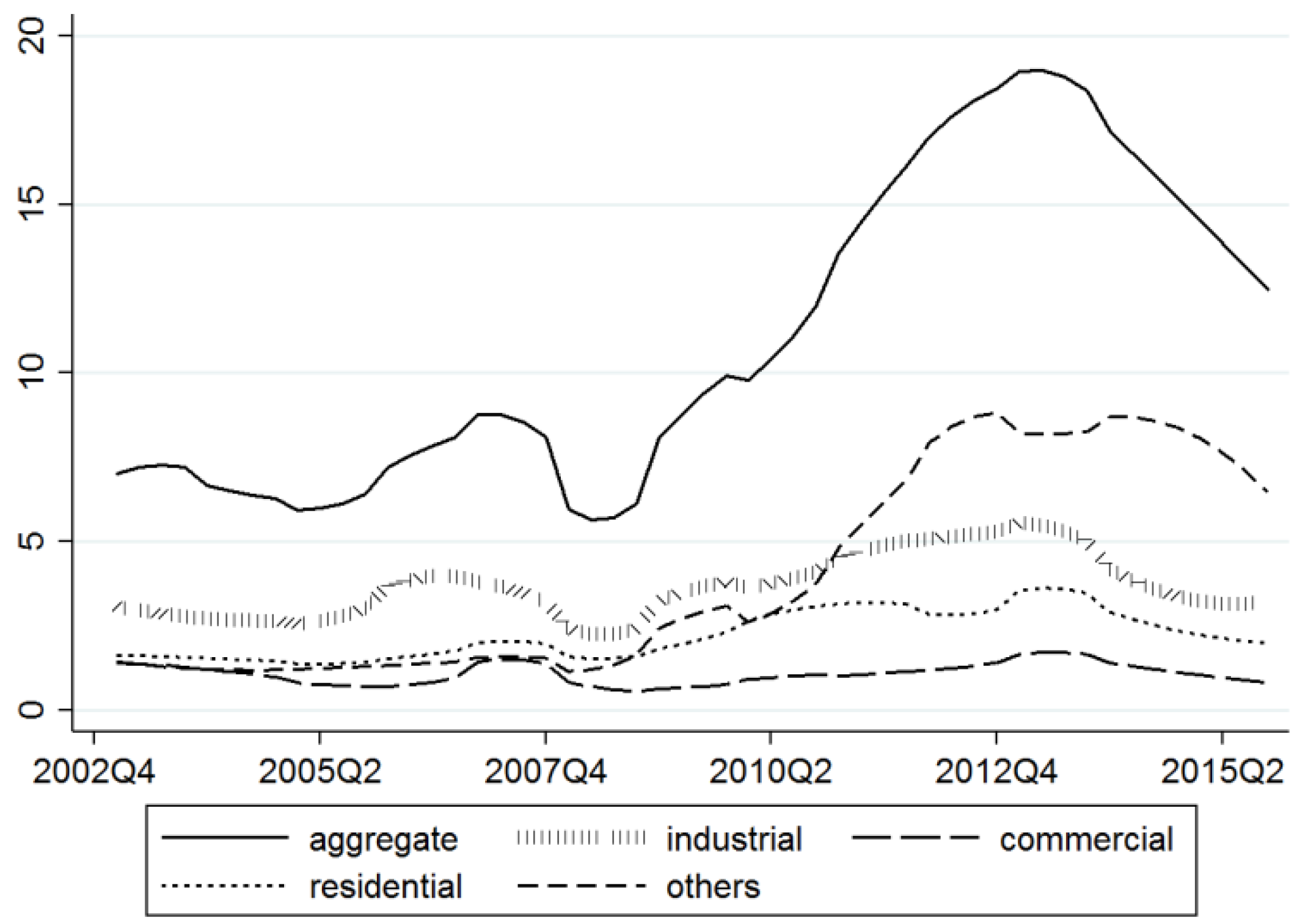
First, as Figure 1 shows, land supply in China is highly cyclical. The correlation between land supply and economic fluctuations can be divided into two periods: from 2003 to 2008 it was about −0.4980, while from 2009 to onward it changed to 0.5158. Such movement applies to various types of land. In Figure 2, I further divide land into four categories and show that they largely move together. Hence, in this paper, I concentrate on the aggregate land supply. I also present correlations between GDP fluctuations and land supply by provincial level data from 2003 to 2014 in

Table 1. Correlations of province-level data.

	2003–2008	2009–2014		2003–2008	2009–2014
Beijing	−0.4321	0.5522	Jiangxi	0.1731	0.5250
Tianjin	−0.2829	0.6659	Shandong	−0.7226	0.1137
Hebei	−0.1272	−0.2077	Henan	0.4657	−0.1378
Shanxi	0.2162	0.6513	Hubei	−0.7393	−0.0436
Inner Mongolia	0.2836	−0.0876	Hunan	−0.4645	0.2663
Liaoning	−0.7199	0.7771	Guangdong	0.2943	−0.3180
Jilin	−0.6314	−0.2737	Guangxi	0.2298	0.2986
Hei Longjiang	−0.0069	0.4189	Hainan	−0.6647	0.5253
Shanghai	−0.7387	0.4606	Chongqing	−0.7877	0.4152
Jiangsu	−0.5729	0.0001	Sichuan	−0.7075	−0.1250
Zhejiang	−0.9580	0.4560	Guizhou	−0.6106	0.6813
Anhui	−0.7664	0.1615	Xizang	0.0474	−0.2823
Fujian	0.5804	0.3544	Yunnan	0.1602	0.0272
Shanxi	−0.3756	0.0315	Gansu	−0.0906	0.2487
Qinghai	−0.0262	0.2477	Ningxia	−0.2555	−0.1926
Xinjiang	−0.1922	0.5383

, which shows co-movement with aggregate data in Figure 1. More specifically, take Hangzhou, which has the highest dependence on land finance, as an example; the correlation coefficient between the supply area of state-owned construction land and the annual GDP growth rate in Hangzhou is −0.2233 from 2005 to 2021. That China’s land supply is highly cyclical sets it apart from many industrialized countries. As a comparison,

Table 2. Year-on-Year growth rate of land (%).

	Std. Dev.	Mean	Min	Max
U.S. (residential)	0.14	0.44	0.25	0.65
China (residential)	22.87	4.61	−26.39	41.36
China (aggregate)	24.80	8.06	−31.52	54.43

calculates and shows that the annualized growth rate of land supply in China is a highly fluctuated variable while that in the U.S. is largely constant (U.S. data comes from [1]). In this paper, I argue that the substantial cyclicality of land supply in China is due to the fact that revenues of selling land have become one of the most important sources of the local government’s income. As

Table 3. Ratio of land sales revenues to local fiscal revenues (%).

2003	2004	2005	2006	2007	2008	2009
57.93	54.30	39.35	44.30	51.96	36.35	53.02
2010	2011	2012	2013	2014	2015
67.74	61.23	45.93	63.53	45.31	37.63

shows, revenues from land sales on average represent about 51.75% of total government income from 2003 to 2014. Consequently, as land prices and tax revenues change with business cycles, land supply in China changes as well.

Second, the relative size of the housing sector in China is large and plays an important role in China’s economy. Specifically, according to the National Bureau of Statistics, the ratio of the real estate industry and construction industry to GDP is 11.39%, contributing to GDP growth by 11.19% from 2003 to 2014. Data from the Ministry of Housing Construction indicates that steel consumption of the real estate industry and construction industry represents about 50% of total steel consumption in China. Motivated by these observations, in the model, I establish a link between the housing sector and the goods in this paper by assuming that the production of housing services requires output from the goods sector as one of its inputs.

Note: GDP series is adjusted by GDP Deflator, log transformed, and detrended with HP filter. The local government supplies land through four channels: free transfer, rent, sale, and others. Measurement of land supply: 10,000 hectares.

Note: “Others” includes the land used for public service, public building, public transportation, water conservancy facility, and special use.

In the model, the cyclical land supply of the local government affects the economy in two ways. First, as in [2], land enters the production function of the goods firm as an input. As a result, fluctuations in the prices and supply of land directly affect the firm’s incentive of acquiring land and adjusting production. I call this the “direct effect” of land policy. Second, as the housing firm also uses output of the goods-producing firm to produce housing services, land prices also affect how much the housing firm sources from the goods firm. Specifically, as the housing firm produces more (less) housing services, demand for the goods firm increases (decreases) accordingly. I call this the “indirect effect” of land policy. I then calibrate the benchmark model to the fluctuations in China’s quarterly data and demonstrate that the calibrated model is able to explain the observed cyclicality of land supply in China. With the calibrated model, I present the impulse responses of a number of key economic variables to illustrate the mechanisms in the benchmark model. I then assess the importance of the two effects of land policy by way of counterfactual exercises.

This paper is most related to two strands of the literature. The first pays attention to the land market and economic fluctuations. These papers argue that monetary policy, geographical position, and unemployment will all affect land price and further economic fluctuations [3,4,5,6,7]. Moreover, enterprises’ collateral channel will amplify the fluctuations of land price and output which may lead to recession [8,9]. Land financing will promote economic growth [10]. If land resources are unevenly distributed, it will hinder economic growth and reduce the efficiency of resource allocation [11], and a higher level of land marketization will lead to more effective land and housing supply [12]. Other related papers in the literature include [13,14,15,16,17,18].

The second strand of the literature studies how the housing market affects the economy. Slow technological progress in the housing sector, productivity, housing premium, household income, and consumption will affect housing fluctuations, and the effect will be amplified by a collateral channel, especially in a unified housing market [19,20,21,22,23,24,25,26,27,28,29,30,31,32]. Improper space allocation, frictional labor markets, and deviation from competitive rent pricing will lead to market distortion [33,34], especially with the development of platform economy [35]. Moreover, housing share can also be used to forecast excess returns on stocks, so that monetary policy, international interest rates, and the current account will be important in the macro-control [36,37,38,39,40].

Different from the literature which has proposed that dynamics in the land market affect final output as it is used by firms as collateral1, this paper studies the link between the land market and China’s macroeconomy by assuming that local governments actively adjust land supply according to their budget constraints2 instead of focusing on the channel of using land as collateral. In addition, I establish a link between the housing sector and the goods sector by assuming that outputs from the goods sector are used as intermediate inputs in producing housing services. Therefore, this paper offers a new possible explanation of the co-movement of the land market, real estate market, and macro-economy from a new perspective of land supply other than land collateral.

The rest of the paper proceeds as follows. Section 2 presents the baseline model. Section 3 presents the details of the quantitative analysis. Section 4 presents three counterfactual exercises to illustrate the relative importance of the two channels I propose in the model, and then I do a robustness check to show the land supply pattern in a social planner problem. Section 5 concludes.

2. The Model

The model makes three extensions to an otherwise standard DSGE model. First, following [2], I assume that household consumes housing services and that land is used as an input in the production of the consumption good. Second, I assume that there is a representative housing firm, which uses land and final consumption goods as intermediate inputs to produce housing services. Last, I include local government in the model, which controls and adjusts land supply in each period. In the model, land does not depreciate and the housing services are fully depreciation, therefore there is no market for second-hand housing trading. Compared with traditional macro-economic models, the DSGE model has micro-foundation in which individuals (e.g., household) make optimal inter-temporal decisions to maximize objective function subject to constraints. Furthermore, the DSGE model contains exogenous shocks, which represent what cause economic fluctuations in real economy (e.g., technological changes, natural disasters, and sudden wars). By this method, this paper can simulate counter-factual experiments for policy evaluation.

2.1. The Representative Household

The representative household has the following utility function:

$$E{\displaystyle \sum _{t=0}^{\infty }{\beta }^t}{A}_t\left[\log (C_t)+{\phi }_t\log (H_t)-{\psi }_t\frac{N_{ht}^{1+\eta }}{1+\eta }\right],$$

(1)

where $C_t$ denotes consumption of final goods, $H_t$ denotes consumption of housing services, $N_{ht}$ denotes labor hours, and $\eta >0$ is the inverse Frisch elasticity of hours worked. The term $A_t$ is a shock to the household’s patience factor, ${\phi }_t$ represents a shock to housing services, and ${\psi }_t$ is a shock to labor supply.

The intertemporal preference shock $A_t$ follows the following stationary process:

$$ln{A}_t=(1-{\rho }_a)ln\overline{A}+{\rho }_{a}ln{A}_{t-1}+{\sigma }_a{\epsilon }_{at},$$

(2)

where $\overline{A}>0$ is a constant, ${\rho }_a\in (0,1)$ measures the degrees of persistence, ${\sigma }_a$ is the standard deviation of the shock, and ${\epsilon }_{at}$ is an i.i.d. standard normal process.

The housing demand shock ${\phi }_t$ follows the following stationary process:

$$ln{\phi }_t=(1-{\rho }_{\phi })ln\overline{\phi }+{\rho }_{\phi }ln{\phi }_{t-1}+{\sigma }_{\phi }{\epsilon }_{\phi t},$$

(3)

where $\overline{\phi }>0$ is a constant, ${\rho }_{\phi }\in (0,1)$ measures the persistence of the shock, ${\sigma }_{\phi }$ is the standard deviation of the shock, and ${\epsilon }_{\phi t}$ is an i.i.d. standard normal process.

The labor supply shock ${\psi }_t$ follows the following stationary process:

$$ln{\psi }_t=(1-{\rho }_{\psi })ln\overline{\psi }+{\rho }_{\psi }ln{\psi }_{t-1}+{\sigma }_{\psi }{\epsilon }_{\psi t},$$

(4)

where $\overline{\psi }>0$ is a constant, ${\rho }_{\psi }\in (0,1)$ measures the persistence of the shock, ${\sigma }_{\psi }$ is the standard deviation of the shock, and ${\epsilon }_{\psi t}$ is an i.i.d. standard normal process.

Let $q_t$ be the price of housing services, $w_t$ be the wage rate, and ${\pi }_t$ and ${\pi }_{ht}$ be the profits from final goods producers and housing firms, respectively. At each $t$, the representative household’s budget constraint is:

$$C_t+q_t{H}_t=w_t{N}_{ht}+{\pi }_t+{\pi }_{ht},$$

(5)

The household’s problem is to choose a sequence of {$C_t$,$H_t$,$N_{ht}$} to maximize (1) subject to (2)–(5), for all $t\ge 0$.

2.2. The Representative Goods Firm

The final goods market is assumed to be perfectly competitive. Carried forward from $t-1$, at each $t$ the entrepreneur is endowed with $K_{t-1}$ units of capital stock and $L_{e,t-1}$ units of land. Output of the representative goods firm is used as intermediate inputs of housing services as well as household’s final consumption good. Its production function is:

$$Y_t=Z_t{\left[L_{e,t-1}^{\varphi }{K}_{t-1}^{1-\varphi }\right]}^{\alpha }{N}_{et}^{1-\alpha },$$

(6)

where $K_t$, $L_{et}$, and $N_{et}$ denote capital, land, and labor, respectively. Total factor productivity (TFP) $Z_t$ follows the stochastic process:

$$ln{Z}_t=(1-{\rho }_z)ln\overline{Z}+{\rho }_{z}ln{Z}_{t-1}+{\sigma }_z{\epsilon }_{zt},$$

(7)

where ${\rho }_z$ measures the degrees of persistence, ${\sigma }_z$ is the standard deviations, and ${\epsilon }_{zt}$ is an i.i.d. standard normal process.

Let $p_t$ denote land price, I assume that, in each period $t$, the firm pays an output tax at the rate $\tau$. It maximizes life-time profits, which can be written as:

$${\displaystyle \sum _{t=0}^{\infty }{\beta }^t}\frac{{\Lambda }_t}{{\Lambda }_0}[(1-\tau )Y_t-K_t+(1-\delta )K_{t-1}-w_t{N}_{et}-p_t(L_{et}-L_{e,t-1})],$$

(8)

where investment follows $I_t=K_t-(1-\delta )K_{t-1}$, and ${\Lambda }_t$ is household’s Lagrange multiplier. The representative firm’s problem is to choose $\left\{K_t,L_{et},N_{et}\right\}$ to maximize (8) at each $t$.

2.3. The Representative Housing Firm

The representative housing firm’s problem is analogous to that solved by the representative goods firm. As the downstream firm and the producer of housing services, the representative housing firm’s production function is:

$$Y_{ht}=M_t^{1-\gamma }{L}_{h,t-1}^{\gamma },$$

(9)

where $M_t$ is intermediate goods produced by the goods firm, and $L_{h,t-1}$ represents land inputs purchased from the local government and accumulated up to $t-1$.

For simplicity, I assume that the housing firm does not pay taxes and the housing services are fully depreciation. Hence, it maximizes life-time profits, which can be written as:

$${\displaystyle \sum _{t=0}^{\infty }{\beta }^t}\frac{{\Lambda }_t}{{\Lambda }_0}[q_t{Y}_{ht}-M_t-p_t(L_{ht}-L_{h,t-1})].$$

(10)

The housing firm’s problem is to choose $\left\{M_t,L_{ht}\right\}$ at each $t$ to maximize (10).

2.4. The Local Government

I assume that the local government maintains a balanced budget at each $t$. In each period, the local government has two sources of revenue: tax receipts and land sales. I denote $G_t$ as the level of government spending at $t$. Its per-period budget constraint is as follows:

$$G_t+u_{L_{et}}+u_{L_{ht}}=\tau Y_t+p_t(L_t^s-L_{t-1}^s).$$

(11)

where $u_{L_{et}}=\frac{\Omega }{2}{(L_{et}-L_{e,t-1})}^2$ and $u_{L_{ht}}=\frac{\Omega }{2}{(L_{ht}-L_{h,t-1})}^2$ are the adjustment costs of land supply which are analogous to [41]. As behavior of the local government plays a crucial role in the model, a detailed discussion is warranted. First, note that government spending is assumed to be exogenously given in the paper. As a result, holding government spending as share of GDP $G_t/Y_t$ constant, land supply ($L_t^s-L_{t-1}^s$) is counter-cyclical. To see this, re-write Equation (11) as follows:

$$(\frac{G_t}{Y_t}-\tau )+\frac{u_{L_{et}}+u_{L_{ht}}}{Y_t}=\left(\frac{p_t}{Y_t}\right)\cdot \left(L_t^s-L_{t-1}^s\right).$$

(12)

Suppose that the economy receives a negative (positive) TFP shock, both land price $p_t$ and output $Y_t$ will decrease (increase). However, one can show that the percentage decrease in land price is always larger than that of the output. As a result, with constant $G_t/Y_t$ and $\tau$, land supply $L_t^s-L_{t-1}^s$ must necessarily increase (decrease). Essentially, this means that, in the model, the local government’s desire to maintain a stable spending share of GDP as well as a balanced budget causes it to adjust land supply counter-cyclically. In equilibrium, the steady-state $\frac{g}{y}>\tau$, and the land supply $\left(L^s-L_{-1}^s\right)>0$ always holds according to the data.

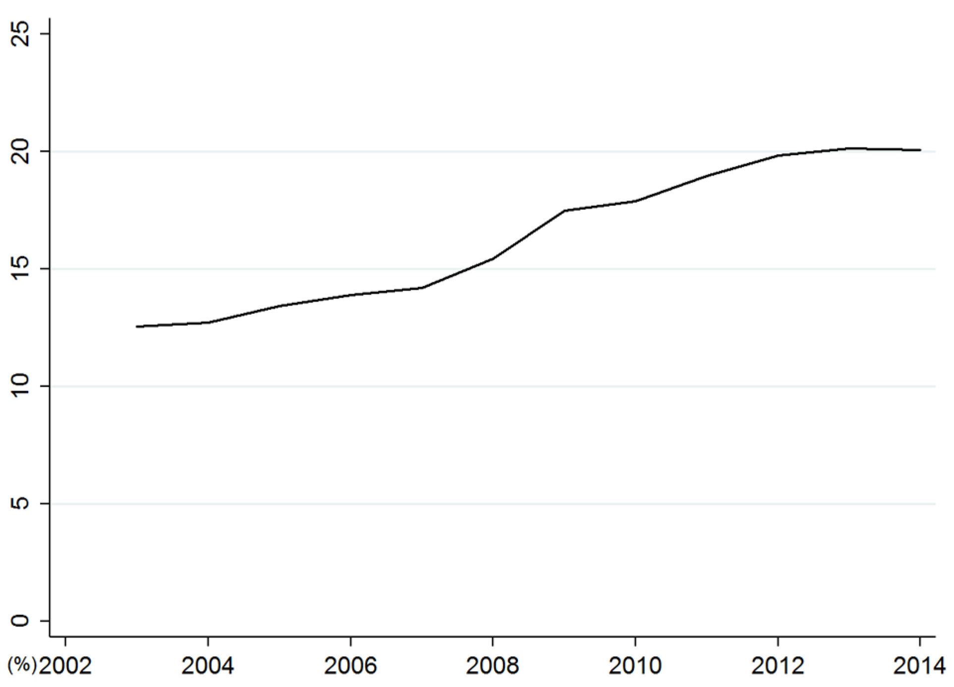
As Figure 1 shows, land supply in China did exhibit strong counter-cyclicality before 2008. However, starting from 2008, it became noticeably pro-cyclical. I believe this is a direct result of the massive spending program, which is often referred to as the “The four-trillion plan”, instituted by the Chinese government in response to the 2008 financial crisis originated from the U.S.3 To see this, one can refer to Figure 3, which shows that local government spending as share of GDP in China was relatively stable before 2008 and started to increase to a substantially higher level after 2008.

In the model, this is reflected as a growing $G_t$ and a declining $Y_t$, which leads to an increasing $G_t/Y_t$. With a constant tax rate $\tau$ and declining $p_t/Y_t$, it must necessarily mean a larger land supply ($L_t^s-L_{t-1}^s$). In other words, in the model, the pro-cyclicality that land supply in China exhibited after 2008 was a result of its local government’s desire to increase spending as share of GDP while maintaining a balanced budget, when the economy experienced negative shocks.

Admittedly, the above representation of the local government’s behavior in China risks over-simplifying what it actually does. However, as shown in the next section, this simplification does a fairly good job at fitting the land supply data and hence captures the essence of the mechanisms explored in this paper. This does not necessarily mean that other government behaviors, such as borrowing by China’s local governments, do not have important implications on China’s macro-economy. Rather, I choose to focus on land supply by the local government in China and leave other potentially important mechanisms to future research.

2.5. Market Clearing Conditions and Equilibrium

In a competitive equilibrium, the markets for goods, labor, land, and housing services all clear. The goods market clearing condition implies that:

$$C_t+K_t-(1-\delta )K_{t-1}+M_t+G_t+u_{L_{et}}+u_{L_{ht}}=Y_t.$$

(13)

The land market clearing condition implies that:

$$L_{et}+L_{ht}=L_t^s.$$

(14)

The housing services market clearing condition implies that:

$$H_t=Y_{ht}.$$

(15)

The labor market clearing condition implies that:

$$N_{ht}=N_{et}=N_t.$$

(16)

A competitive equilibrium consists of sequences of prices $\{w_t,q_t,p_t\}$ and allocations $\{C_t,H_t,N_{ht}, N_{et},L_{et},L_{ht},L_t^s,M_t,K_t,Y_t,G_t\}$ such that (i) taking prices and tax rate as given, the allocations solve the optimizing problems of the household, the goods firm, and the housing firm; (ii) the local government’s budget (11) is satisfied; and (iii) all markets clear.

3. Calibration and Estimation

Calibration of the model proceeds as follows. First, I log-linearized the model around the steady state. Second, I fit the log-linearized model to four quarterly time series in China: the real price of housing services, real per capita household consumption, real per capita GDP, and number of employees4. I then show the mechanism by impulse response. The sampled period ranges from 2003:Q1 to 2014:Q4. Data on China’s macroeconomy are taken from WIND Database, Ministry of Land and Resources, and China Statistical Yearbook.

3.1. Parameter Values and Steady-States

I solve the model numerically based on calibrated parameters. I partition the model parameters into two subsets. The first subset of parameters includes the structural parameters, which are calibrated using the steady-state relations. This set of parameters is collected in

Table 4. Values of parameters.

Parameter	Description	Value
$\alpha$	Share of capital and land in firm’s production	0.5
$\beta$	Subjective discounting factor	0.99
$\eta$	Inverse Frisch elasticity	2
$\gamma$	Share of land in housing sector’s production	0.5
$\varphi$	Share of land relative to capital in firm’s production	0.0697
$\tau$	Steady state of tax rate of local government	0.0760
$\delta$	Steady state of depreciation rate	0.0250
$\frac{c}{y}$	Steady state of consumption-output ratio	0.3795
$\frac{g}{y}$	Steady state of local government spending-output ratio (before 2008)	0.1369
$\frac{g}{y}$	Steady state of local government spending-output ratio (after 2008)	0.1906
$\frac{pl}{y}$	Steady state of land sales-output ratio	0.0943
$\frac{l_h}{l}$	Steady state of residential land-total land supply ratio	0.2168

. Calibration is commonly used in macro quantitative analysis. It selects the fitting target through macro-data, and then calculates the relevant parameter values that can reach the fitting target in the model. The calibration parameters make the theoretical model consistent with the real data, which is helpful to predict the dynamic transition of macro-economy under shocks.

As is standard in the literature, I fix the subjective discount factor $\beta$ at 0.99. I select 0.5 for $\alpha$, which is consistent with empirical evidence in Chinese data [42,43]. For the utility function parameters, I set $\eta =2$, implying a Frisch elasticity of labor supply of 0.5, consistent with microeconomic evidence [44]. I select 0.5 for $\gamma$, which determines the share of land in the production of housing services. This value is consistent with the estimates of intermediate input share in U.S. data by [45] and was subsequently used in studies on China’s macroeconomy such as [44]. Following [2], I select 0.0697 for $\varphi$ as the share of land relative to capital in firm’s production. I set the tax rate $\tau =0.0760$ according to China Statistical Yearbook, as it is the average share of tax receipts in China’s local government budgets in the sampled period. Lastly, I select 0.025 for the capital depreciation rate $\delta$ as it is the value commonly used in the literature. Moreover, I calculate last five steady-state moments in Table 4 based on data of consumption, local government spending, output, land sales revenues, and land supply from WIND Database, Ministry of Land and Resources, and China Statistical Yearbook.

3.2. Estimating Shocks

To match the model to the fluctuations observed in the data, I follow the approach in [43,46], in which the authors propose a Bayesian method to estimate the parameters of shocks. Bayesian estimation is also widely used. It constructs a Markov process with a stable transition distribution in a space, makes the parameters of the model approach the stable distribution of the chain by finding an appropriate Markov chain transition equation, and calculates the Monte Carlo integration by using the sampling points in the steady distribution, and then infers the peak, skewness, mean, and variance. This is a parameter estimation method based on Bayesian statistical theory, which is mainly used to generate posteriori distributed samples. Moreover, I refer to [2,41] for the prior distributions.

Table 5. Parameter estimations.

Parameter	Distribution	Prior	Std. Dev.	Posterior	90% Probability Interval
${\rho }_a$	Beta	0.5000	0.2000	0.9129	[0.8554, 0.9719]
${\rho }_{\phi }$	Beta	0.5000	0.2000	0.4107	[0.2254, 0.6034]
${\rho }_{\psi }$	Beta	0.5000	0.2000	0.9109	[0.8369, 0.9944]
${\rho }_z$	Beta	0.5000	0.2000	0.7798	[0.6896, 0.8844]
${\epsilon }_a$	InvGamma	0.0100	Inf	0.0079	[0.0061, 0.0100]
${\epsilon }_{\phi }$	InvGamma	0.0100	Inf	0.0829	[0.0693, 0.0986]
${\epsilon }_{\psi }$	InvGamma	0.0100	Inf	0.0107	[0.0092, 0.0126]
${\epsilon }_z$	InvGamma	0.0100	Inf	0.0092	[0.0079, 0.0107]

reports the estimates of structural parameters at the posterior mode. I also report the 90% probability intervals for model parameters in the table. One can see from Table 5 that the estimated shocks are persistent and have large standard deviations.

3.3. Impulse Responses

Impulse response can clearly show the response path of the economic system to the impact (i.e., shocks) from a certain moment in the present and future. The impulse response cares about how indeterministic items affect key variables, and the lag order needs to be set for the impulse response.

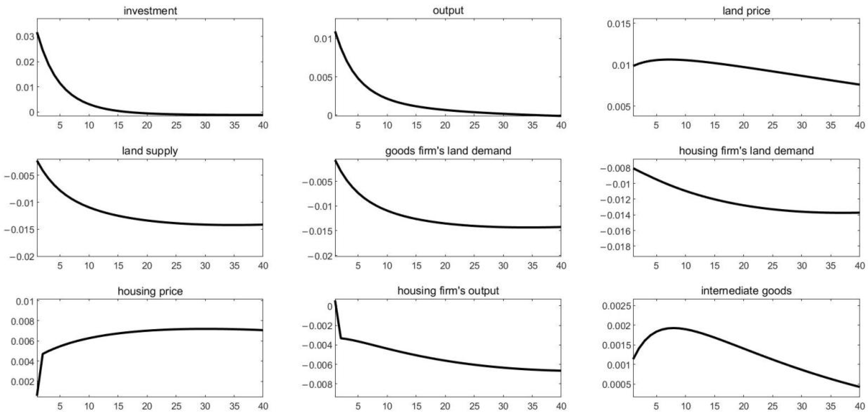
Figure 4 shows the impulse responses of nine key macroeconomic variables following a positive (one standard deviation) TFP shock. Not surprisingly, output increases after a positive TFP shock. Both land price and the price of housing services increase as a result. As described by Equation (11), local government reduces its land supply following the TFP shock.

Endogenous land supply dampens the business cycle both directly and indirectly. Such dampening effect has directly led to the U-shaped demand for land curves of both the goods firm and the housing firm. Initially, the positive TFP shock causes land price to increase. The counter-cyclical nature of the local government’s behavior means that land supply decreases as a result. Because land is an input in the production of both the goods firm and the housing firm, a decrease in land supply directly impacts output negatively. Consequently, the positive stimulating effect of a TFP shock is dampened. This is the “direct effect” of the endogenous land supply. On the other hand, the “indirect effect” works through the intermediate goods market. After a positive TFP shock hits the economy, the endogenously falling land supply and the resulting rising land prices partially offset the housing firm’s incentive of increasing its output. As output of the goods firm is also used as input of housing service, this means that demand for final good decreases after the initial increase.

4. Counterfactual Exercises

In this section, I perform three counterfactual exercises based on the calibrated benchmark model. The goal is to assess, quantitatively, how endogenous land supply and the linkage between the housing sector and the goods sector impact China’s business cycles. First, by assuming that the production of housing services does not use any intermediate inputs from the goods firm, I study the “indirect effect”, which works through the intermediate inputs market. The second exercise studies the role of endogenous land supply. Specifically, I assume that the local government maintains a fixed land supply, instead of actively adjusting land supply as in the baseline model. In this case, tax rate on the goods firm is allowed to vary in order the keep a balanced government budget. In the last counterfactual exercise, I shut down both channels to see how the business cycles in China would change when land supply is fixed and that the linkage between the housing sector and the goods sector ceases to exist.

Table 6. Std. Dev. of GDP summary $Y_t$ (%).

		Std. Dev.	$\frac{\mathit{b}\mathit{a}\mathit{s}\mathit{e}\mathit{l}\mathit{i}\mathit{n}\mathit{e}}{\mathit{c}\mathit{o}\mathit{u}\mathit{n}\mathit{t}\mathit{e}\mathit{r}\mathit{f}\mathit{a}\mathit{c}\mathit{t}\mathit{u}\mathit{a}\mathit{l}}.$
	China’s data	1.7116	-
1	baseline model	1.7767	-
2	Endogenous land supply, no intermediate goods	4.8483	36.65%
3	Exogenous land supply, with intermediate goods	5.3428	33.25%
4	Exogenous land supply, no intermediate goods	5.3489	33.21%

provides a summary of the results of the counterfactual exercises.

4.1. Case One: Endogenous Land Supply and $\gamma =1$

In this counterfactual, I shut down the channel by which the housing sector affects the goods sector through intermediate inputs. I achieve this by setting $\gamma =1$ in Equation (9). Hence, it becomes:

$$Y_{ht}=L_{ht}.$$

(17)

Doing so allows us to completely shut down the “indirect effect”, which works through the intermediate inputs market. A comparison between the counterfactual exercise (without linkage) and benchmark model shows that, in general, business cycles become more pronounced as a result. To observe the changes of key variables, I simulate the calibrated model by assuming a one standard deviation positive TFP shock. As shown in Figure 5, the changes of housing service and housing service prices are larger compared to the benchmark case. As a result of the larger decrease in housings service, the increase of housing service price is larger.

What are the implications of these larger changes in housing service and housing services price on China’s business cycles? I answer this question by replacing Equation (9) with Equation (17), while keeping all the shocks estimated in the calibrated model. As Table 6 shows, the standard deviation of output jumps from 1.7767 to 4.8483 as a result. This shows that having a linkage between the housing sector and the goods sector will lead to smaller fluctuation in output.

4.2. Case Two: Fixed Land Supply and $\gamma <1$

To explore the role of the “direct effect”, I consider the case that land supply by the local government is fixed to $\overline{L}$. In this case, two changes need to be made. First, the local government’s budget constraint becomes:

$$G_t={\tau }_t{Y}_t,$$

(18)

Moreover, land market clearing condition implies that:

$$L_{et}+L_{ht}=\overline{L}.$$

(19)

Figure 6 shows the changes in the case of fixed land supply and the impulse responses following one standard deviation positive TFP shock. As Figure 6 indicates, it takes longer for the changes of output to fall back to zero compared to the baseline model (over 40 quarters in Figure 6 vs. 35 quarters in Figure 4). Changes of housing services become positive as a result of the fixed land supply because the land is reallocated between both firms and not actively adjusted by the government. Another important observation is that, to keep Equation (18) balanced, tax rate declines, which will further amplify economic fluctuations.

What are the implications of fixed land supply on China’s business cycles? I answer this question by assuming fixed land supply in the counterfactual, while keeping all the shocks estimated in the calibrated model. As Table 6 shows, the standard deviation of output increases from 1.7767 to 5.3428 as a result. This shows that having fixed land supply will lead to much larger fluctuations in output.

4.3. Case Three: Fixed Land Supply and $\gamma =1$

What if I shut down both the “direct effect” and the “indirect effect”? I answer this question by combining case one and two. In Figure 7, I find that the persistence of output is much larger. Moreover, declining tax rate will further amplify economic fluctuations.

To examine the implications on China’s business cycles, I assume no linkages between the housing sector and the goods sector and that land supply is fixed, while keeping all the shocks estimated in the calibrated model. As shown in Table 6, while the three counterfactual exercises all generate larger standard deviations in real GDP, the last one in which both channels are absent generates the most pronounced business cycles. I therefore conclude from the counterfactual exercises that both of the two particular channels considered in this paper tend to cause China’s business cycles to be less pronounced.

4.4. Welfare Analysis: The Optimal Land Supply Policy

Next, I compare the macro implications of the fix land supply policy regime relative to the benchmark regime of the endogenous land supply policy. I measure welfare gains under the counterfactual policy relative to the benchmark model as the percentage change in permanent consumption that would leave the representative household indifferent between living in an economy under the fix land supply policy and in the benchmark economy. The result shows that endogenous land supply policy can increase social welfare by about 1.38%. This implies that by endogenous land supply, the government is able to dampen the business cycle both directly and indirectly, leading to superior outcomes for welfare than fix land supply policy.

4.5. Robustness Check: Social Planning Problem

In the benchmark model, I suppose that the local government adjusts actively the land supply according to the $\frac{G_t}{Y_t}$ ratio, and it is kind of an exogenous assumption. Now, I try to formulate a social planning problem which generates the endogenous land supply that maximizes social welfare, and I find that the counter-cyclical land supply pattern is still robust. The detailed model and results are shown in Appendix A.

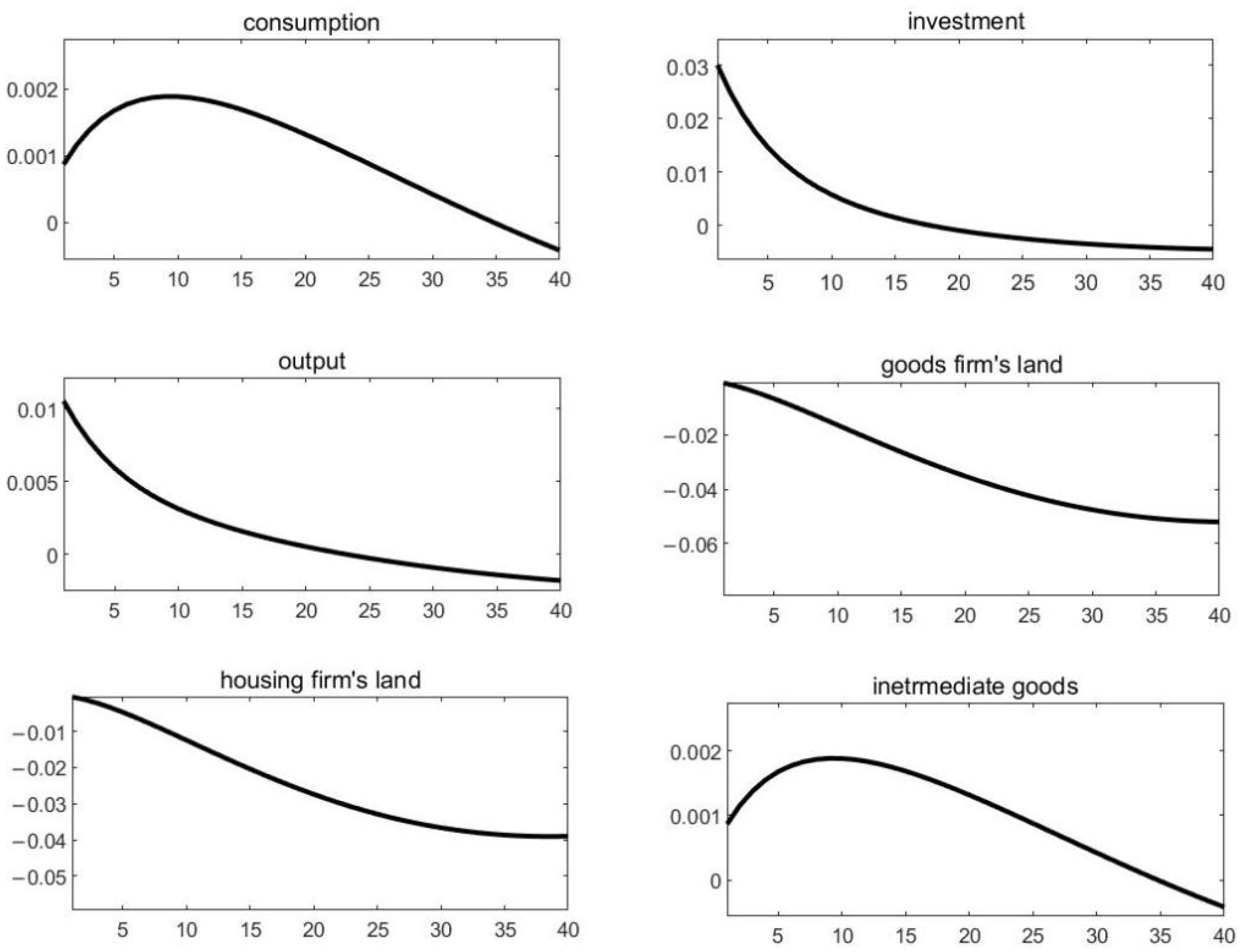
As a positive TFP shock increases the intertemporal substitution elasticity $E_t\beta \frac{C_t}{C_{t+1}}$5. Therefore, a positive TFP shock increases the right hand side (marginal cost) larger than the left hand side (marginal benefit). The social planner (local government) will decrease land supply $L_{et}$ and $L_{ht}$ to equate both the equations. Similarly, a negative TFP shock leads to increasing land supply $L_{et}$ and $L_{ht}$.

In Figure 8, I show the key variables’ impulse responses following a one standard deviation of positive TFP shock. A positive shock increases consumption, final goods firm’s investment, and output, obviously. According to Equations (A15) and (A16), the marginal cost exceeds the marginal revenue at the time and therefore the government decreases both the goods firm and housing firm’s land supplies. This implies that the counter-cyclical pattern of land supply is still robust in an endogenous social planner’s problem.

4.6. Discussion

This paper explores the counter-cyclical relationship between land supply and economic fluctuations. The main mechanism argued in this paper can be verified by a series of documents of the Chinese government.

Table 7. Chronology of structural changes.

Dates	Major Structural Changes	The Condition of China	Document Effect
2003	Document from State Council NO.18 [2003]	Overheated investment in real estate	Tighten land supply and make housing market and economy less pronounced
2004	Document from State Council NO.28 [2004]	Overheated investment in real estate
2005	Document from State Council NO.26 [2005]	Rapid decline in the real estate market growth	Increase land supply and simulate real estate investment
2008	“The four-trillion” plan	Financial crisis	Land supply kept relatively loose to simulate economy
2010	Document from State Council NO.04 [2010]	Two years after financial crisis

displays major structural changes from 2003 onward. In 2003, the year-on-year growth of real estate investment was as high as 30.3%, so the State Council issued a document named “Circular of the State Council on Promoting the Sustained and Sound Development of Real Estate Market” (No.18, [2003]) and set a tone of “strict management of land and keep tight credit” to control the overheated investment in real estate. “Decision of the State Council on Deepening the Reform and Exercising Strict Land Administration” (No.28, [2004]) was published continuously. Both documents were aimed to tighten land supply and make the economy less pronounced. The two documents had substantial effects on the land and housing market, and investment declined heavily as a result. Under strict policy control, the growth rate of real estate investment slowed down further in 2005, and the proportion of real estate investment in fixed assets investment dropped rapidly from the peak 51.33% to 17.8% in 2005. So followed by a document named “Circular of the General Office of the State Council on Transmitting and Issuing the Proposals of the Ministry of Construction and Other Departments for Stabilizing the Housing Price” (No.26, [2005]) in 2005, the government targeted to simulate economy and planned to increase land supply. At the end of 2006, national real estate investment rate increased back to 21.8%.

After the 2008 financial crisis, to coordinate with “The four-trillion plan”, land supply was kept relatively loose to help improve economic recovery. A good example was the document “Circular of the General Office of the State Council on Pushing Forward the Stable and Sound Development of the Real Estate Market” (No.04, [2010]). Data from IMF’s World Economic Outlook shows that the recent 2008 financial crisis brought down the GDP growth rate of the U.S. sharply to −3.5% in 2009, as well as Germany (−5.1%), France (−2.6%), Britain (−4.4%), Canada (−2.8%), Japan (−5.5%), and so on. Russia was the worst (−7.8%) in the BRIC countries in 2009; others such as Brazil and South Africa reached −0.3% and −1.5%, respectively. However, China’s GDP growth rate greatly achieved 9.6%, 9.2%, and 10.4% from 2008 to 2010, ranking the second largest economy surprisingly. Such rapid growth may likely have something to do with the distinct China’s land policy. The real estate market has a great impact on economic growth, which has been confirmed by many literature studies [2,41,47,48]). Land supply will affect land price, as well as housing price and housing premium, and the effect will be amplified by housing collateral [19,31]. As a result, the impact of land supply on the economy will eventually be transmitted to family wealth and social welfare [37,49]. Moreover, land supply policy can affect the formulation and implementation of fiscal and monetary policies through land mortgage, so comprehensive macro control policy is needed [17,50]. As land supply is a very important policy, although I study the Chinese economy in quantitative analysis, I believe that the findings are applicable to a much larger group of countries, where the housing sector is large relative to the overall economy or that (local) governments at various levels can actively adjust land supply (e.g., Singapore, Chinese Hong Kong).

5. Conclusions and Policy Implications

5.1. Conclusions

In this paper, I first present evidence that China’ land supply is highly cyclical. I argue that this is mainly due to the fact that local governments in China actively adjust land supply to maintain their budgets. Moreover, I argue that it is important to consider how the large share of the housing sector in the overall Chinese economy could have implications on its business cycles.

To study the roles of these two factors, I construct a DSGE model that incorporates endogenous land supply and a housing sector that uses output of the goods sector in producing housing services. In the model, the cyclical land supply by the local government affects the economy in two ways. First, land enters the production function of the goods firm as an input. As a result, fluctuations in the prices of land directly affect firms incentive of acquiring land and adjusting production. I call this the “direct effect” of land policy. Second, as the housing firm uses land to produce housing services, the housing firm produces more (less) housing services, and demand for the goods firm increases (decreases) accordingly. I call this the “indirect effect” of land policy. I then calibrate the model to the fluctuations by four quarterly China time series.

By way of counterfactual exercises, I find that both mechanisms I study in the model tend to dampen the business cycles in China. GDP fluctuations increase by 63.35% without “indirect effect”, increase by 66.75% without “direct effect”, and increase by 66.79% without both effects. Moreover, endogenous land supply policy can increase social welfare by about 1.38%.

5.2. Policy Implications

Verifying by the stylized facts in China, this paper finds that endogenous land supply is an efficient macro-control policy to smooth the economy and increase social welfare. This paper argues that the government should: first strengthen the monitoring of the land market and the statistical analysis of the real estate market, and put forward timely land policies in view of the latest economic situation. During economic recession, appropriately increase land supply to stimulate real estate and real economy investment; while during economic prosperity, tighten land supply and make good use of the counter-cyclical land supply policy to ensure stable economic growth. Second, the government should strengthen land supply management, comprehensively consider land supply, supply structure, development time limit and idle land ratio, reasonably determine land supply, and explore reasonable land transfer methods. Third, in the process of land supply, the government should try to avoid the problem of rent-seeking in the land market and the problem of excessive growth of local government land mortgage financing loans. Land rent-seeking will lead to resource misallocation and social welfare loss. With the increasing balance of local government financing, its repayment pressure and the risk of default are gradually increasing as well.

This paper does not distinguish land types. In practice, although the fluctuation trend of various types of land is similar, their impacts are completely different. The price of commercial and residential land is high, but the supply area is relatively low. However, the price of industrial land is low and its supply area accounts for a large proportion. Therefore, it is important to divide different types of land and incorporate them into the heterogeneous DSGE model in the future. Moreover, with the in-depth development of the world economy, exchanges between countries have become increasingly frequent. All countries are inevitably affected by the world economic environment. China is no exception. Since China joined the WTO in 2001, its economy has become more and more open. Therefore, expanding the DSGE model in open economy is also a promising direction for further research.

References

- Davis, M.A.; Heathcote, J. The Price and Quantity of Residential Land in the United States. J. Monet. Econ. 2007, 54, 2595–2620. [Google Scholar] [CrossRef]
- Liu, Z.; Wang, P.; Zha, T. Land-Price Dynamics and Macroeconomic Fluctuation. Econometrica 2013, 81, 1147–1184. [Google Scholar]
- Kwon, E. Monetary Policy, Land Prices, and Collateral Effects on Economic Fluctuations: Evidence from Japan. J. Jpn. Int. Econ. 1998, 12, 175–203. [Google Scholar] [CrossRef]
- Saiz, A. The Geographic Determinants of Housing Supply. Q. J. Econ. 2010, 125, 1253–1296. [Google Scholar] [CrossRef]
- Miao, J.; Wang, P.; Zhou, J. Housing Bubbles and Policy Analysis; Working Paper; Boston University: Boston, MA, USA, 2014. [Google Scholar]
- Liu, Z.; Miao, J.; Zha, T. Land Prices and Unemployment. J. Monet. Econ. 2016, 80, 86–105. [Google Scholar] [CrossRef]
- Du, X.; Huang, Z. How Does The G20 Summit Affect Land Market? Evidence from China. Int. J. Strateg. Prop. Manag. 2021, 25, 432–445. [Google Scholar] [CrossRef]
- Kiyotaki, N.; Moore, J. Credit Cycles. J. Political Econ. 1997, 105, 211–248. [Google Scholar] [CrossRef]
- Gan, J. Collateral, Debt Capacity, and Corporate Investment: Evidence from a Natural Experiment. J. Financ. Econ. 2007, 85, 709–734. [Google Scholar] [CrossRef]
- Mo, J. Land Financing and Economic Growth: Evidence from Chinese Counties. China Econ. Rev. 2018, 50, 218–239. [Google Scholar] [CrossRef]
- Chen, C.; Restuccia, D.; Santaeulàlia-Llopis, R. The Effects of Land Markets on Resource Allocation and Agricultural Productivity; NBER Working Paper 24034; National Bureau of Economic Research: Cambridge, MA, USA, 2021.
- Li, L.; Bao, X.H.; Robinson, G.M. The Return of State Control and Its Impact on Land Market Efficiency in Urban China. Land Use Policy 2020, 99, 104878. [Google Scholar] [CrossRef]
- Greenwood, J.; Hercowitz, Z.; Krusell, P. Long-Run Implications of Investment-Specifific Technological Change. Am. Econ. Rev. 1997, 87, 342–362. [Google Scholar]
- Christiano, L.; Eichenbaum, M.; Evans, C. Nominal Rigidities and the Dynamics Effects of a Shock to Monetary Policy. J. Political Econ. 2005, 113, 1–45. [Google Scholar] [CrossRef] [Green Version]
- Campbell, J.R.; Hercowitz, Z. The Role of Collateralized Household Debt in Macroeconomic Stabilization; NBER Working Paper Series, No. 11330; National Bureau of Economic Research: Cambridge, MA, USA, 2006.
- Taylor, J.B. Housing and Monetary Policy; NBER Working Paper Series, No. 13682; National Bureau of Economic Research: Cambridge, MA, USA, 2007.
- He, C.; Wright, R.; Zhu, Y. Housing and Liquidity. Rev. Econ. Dyn. 2014, 18, 435–455. [Google Scholar] [CrossRef]
- Chaney, T.; Sraer, D.; Thesmar, D. The Collateral Channel: How Real Estate Shocks Affect Corporate Investment. Am. Econ. Rev. 2012, 102, 2381–2409. [Google Scholar] [CrossRef]
- Case, K.E. Real Estate and the Macroeconomy. Brook. Pap. Econ. Act. 2000, 31, 119–162. [Google Scholar] [CrossRef]
- Glaeser, E.L.; Gyourko, J.; Saks, R. Why Have Housing Prices Gone Up? Am. Econ. Rev. Pap. Proc. 2005, 95, 329–333. [Google Scholar] [CrossRef]
- Lustig, H.; Nieuwerburgh, S.V. Housing Collateral, Consumption Insurance and Risk Premia: An Empirical Perspective. J. Financ. 2005, 60, 1167–1219. [Google Scholar] [CrossRef]
- Sinai, T.; Souleles, N.S. Owner-Occupied Housing as a Hedge Against Rent Risk. Q. J. Econ. 2005, 120, 763–789. [Google Scholar]
- Ortalo-Magnè, F.; Rady, S. Housing Market Dynamics: On the Contribution of Income Shocks and Credit Constraints. Rev. Econ. Stud. 2006, 73, 459–485. [Google Scholar] [CrossRef]
- Iacoviello, M. House Prices, Borrowing Constraints, and Monetary Policy in the Business Cycle. Rev. Econ. Dyn. 2005, 95, 739–764. [Google Scholar] [CrossRef]
- Iacoviello, M.; Neri, S. Housing Market Spillovers: Evidence from an Estimated DSGE Model. Am. Econ. J. Macroecon. 2010, 2, 125–164. [Google Scholar] [CrossRef]
- McCarthy, J.; Steindel, C. Housing Activity and Consumer Spending. Bus. Econ. 2007, 42, 6–21. [Google Scholar] [CrossRef]
- Campbell, J.; Cocco, J. How Do House Prices Affect Consumption? Evidence from Micro Data. J. Monet. Econ. 2007, 54, 591–621. [Google Scholar] [CrossRef] [Green Version]
- Campbell, S.D.; Davis, M.A.; Gallin, J.; Martin, R.F. What Moves Housing Markets? A Variance Decomposition of the Rent-Price Ratio. J. Urban Econ. 2009, 66, 90–102. [Google Scholar] [CrossRef]
- Kahn, J.A. What Drives Housing Prices? Fed. Reserve Bank N. Y. Staff Rep. 2008, 626, 1–42. [Google Scholar] [CrossRef]
- Wu, J.; Gyourko, J.; Deng, Y. Is There Evidence of a Real Estate Collateral Channel Effect on Listed Firm Investment in China? NBER Working Paper Series, No. 18762; National Bureau of Economic Research: Cambridge, MA, USA, 2013.
- Fang, H.; Gu, Q.; Xiong, W.; Zhou, L. Demystifying the Chinese Housing Boom; NBER Working Paper 21112; National Bureau of Economic Research: Cambridge, MA, USA, 2015.
- An, G.; Becker, C.; Chen, E. Housing Price Appreciation and Economic Integration in A Transition Economy: Evidence from Kazakhstan. J. Hous. Econ. 2021, 52, 101765. [Google Scholar] [CrossRef]
- Chapelle, G.; Wasmer, E.; Bono, P.H. An Urban Lbor Market with Frictional Housing Markets: Theory and An Application to The Paris Urban Area. J. Econ. Geogr. 2021, 21, 97–126. [Google Scholar] [CrossRef]
- Maynou, L.; Monfort, M.; Morley, B.; Ordóez, J. Club Convergence in European Housing Prices: The Role of Macroeconomic and Housing Market Fundamentals. Econ. Model. 2021, 103, 105595. [Google Scholar] [CrossRef]
- Shabrina, Z.; Arcaute, E.; Batty, M. Airbnb and Its Potential Impact on The London Housing Market. Urban Stud. 2022, 59, 197–221. [Google Scholar] [CrossRef]
- Aoki, K.; Proudman, J.; Vlieghe, G.W. House Prices, Consumption, and Monetary Policy: A Financial Accelerator Approach. J. Financ. Intermediation 2004, 13, 414–435. [Google Scholar] [CrossRef]
- Piazzesi, M.; Schneider, M.; Tuzel, S. Housing, Consumption, and Asset Pricing. J. Financ. Econ. 2007, 83, 531–569. [Google Scholar] [CrossRef]
- Favilukis, J.; Ludvigson, S.; Nieuwerburgh, S. The Macroeconomic Effects of Housing Wealth, Housing Finance, and Limited Risk-Sharing in General Equilibrium. J. Political Econ. 2017, 125, 140–223. [Google Scholar] [CrossRef]
- Franjo, L. International Interest Rates, The Current Account and Housing Markets. Econ. Model. 2018, 75, 268–280. [Google Scholar] [CrossRef]
- Li, S.; Suardi, S.; Wee, B. Bank Lending Behavior and Housing Market Booms: The Australian Evidence. Int. Rev. Econ. Financ. 2022, 819, 184–204. [Google Scholar] [CrossRef]
- Iacoviello, M. Financial Business Cycles. Rev. Econ. Dyn. 2015, 18, 140–163. [Google Scholar] [CrossRef]
- Brandt, L.; Hsieh, C.T.; Zhu, X. Growth and Structural Transformation in China. In China’s Great Economic Transformation; Brandt, L., Rawski, T.G., Eds.; Cambridge University Press: Cambridge, UK, 2008. [Google Scholar]
- Miao, J.; Wang, P.; Xu, Z. A Bayesian Dynamic Stochastic General Equilibrium Model of Stock Market Bubbles and Business Cycles. Quant. Econ. 2015, 6, 599–635. [Google Scholar] [CrossRef]
- Chang, C.; Liu, Z.; Spiegel, M.M. Capital Controls and Optimal Chinese Monetary Policy. J. Monet. Econ. 2015, 74, 1–15. [Google Scholar] [CrossRef]
- Basu, S. Intermediate Goods and Business Cycles: Implications for Productivity and Welfare. Am. Econ. Rev. 1995, 85, 512–531. [Google Scholar]
- Sims, C.A.; Zha, T. Bayesian Methods for Dynamic Multivariate Models. Int. Econ. Rev. 1998, 39, 949–968. [Google Scholar] [CrossRef]
- Miao, J.; Wang, P.; Zha, T. Liquidity Premia, Price-Rent Dynamics and Business Cycles; Working Paper; Boston University: Boston, MA, USA, 2014. [Google Scholar]
- Li, X.; Hui, C.M.; Shen, J. The Consequences of Chinese Outward Real Estate Investment: Evidence from Hong Kong Land Market. Habitat Int. 2020, 98, 102151. [Google Scholar] [CrossRef]
- Arestis, P.; Zhang, S. Are There Irrational Bubbles under The High Residential Housing Prices in China’s Major Cities? Panoeconomicus 2020, 67, 1–26. [Google Scholar] [CrossRef]
- Chen, C.; Chiang, S. Time-varying Spillovers Among First-tier Housing Markets in China. Urban Stud. 2020, 57, 844–864. [Google Scholar] [CrossRef]
Figure 1.
Business cycles of GDP and land supply.
Figure 2.
Various types of land supply (measurement: 10,000 hectares).
Figure 3.
The ratio of local government spending to GDP.
Figure 4.
Impulse responses to a positive (one standard deviation) TFP shock (endogenous land, 1).
Figure 5.
Impulse responses to a positive (one standard deviation) TFP shock (endogenous land, = 1).
Figure 6.
Impulse responses to a positive (one standard deviation) TFP shock (fix land, < 1).
Figure 7.
Impulse responses to a positive (one standard deviation) TFP shock (fix land, = 1).
Figure 8.
Impulse responses to a positive (one standard deviation) TFP shock in social planner’s problem.