Evaluating Ecosystem Services for the Expansion of Irrigation on Agricultural Land

Abstract

Managing water resources requires consideration of both environmental and socio-economic benefits to effectively balance the benefits and costs. This includes identifying ecosystem services (ES) of concern and how to evaluate the project or proposed changes effect on these ES. The purpose of this effort is to describe methods to evaluate ecosystem services to provide expanded irrigation to existing agricultural lands in Alabama and the potential application to other areas. A case study has been undertaken on the Middle Alabama watershed in central Alabama and methods have been developed and applied to evaluate ES in terms of how irrigated versus rainfed fields will affect sediment retention, fertilizer usage and the effect of the subsequent discharges of sediment and nitrogen from fertilizer on water quality. The results of case studies in the Middle Alabama watershed indicate positive ES benefits from sustainable agricultural practices and the irrigation of agricultural lands versus rainfed fields. We anticipate these methods will be applicable to other watersheds outside the southeast region too.

1. Introduction

While the annual precipitation rate in Alabama averages 1400 mm, annual rates typically ranged from 1140 to 1605 mm since 1900 with rates as low as 890 mm in some years. In addition, growing season precipitation is highly variable, and climate change is expected to intensify the hydrologic cycle. Though there is still a lot of uncertainty, trends for growing seasonal precipitation in the growing season show an inclination towards slightly drier conditions [1]. Due to the highly variable summer precipitation in Alabama, irrigation can be a key adaptation strategy to bolster agricultural resilience [2] well as a mitigation strategy against climate change.

To that end, a federally funded initiative was begun in 2017 to encourage farmers in the state to irrigate existing agricultural land by sharing the cost of irrigation facilities. The Alabama Natural Resources Conservation Service (NRCS) is working with the Sponsoring Local Organization (SLO), Alabama Soil and Water Conservation Committee (ASWCC), to allocate Public Law 83-566 “Watershed Protection and Flood Prevention Act” (henceforth referred to as PL-566) funding to support this ongoing program, the Alabama Irrigation Project (AIP). As a federally funded initiative, the execution of the program requires that an environmental impact assessment and a cost-benefit analysis be performed. This is being done by scientists at Auburn University and the University of Alabama in Huntsville. The program is being executed across the state at the large watershed (HUC-8) level. Currently, the Middle Alabama basin is under investigation and activities in this basin form the basis of this manuscript.

Potential benefits (or costs) of irrigation involves impacts on ecosystem services including soil health and water quality. A crop that does not mature properly due to lack of moisture does not efficiently uptake nutrients, contributing to residual nutrients to be lost to surface or groundwater during rains. Additionally, a crop that does not mature reduces the amount of organic matter available for incorporation into the soil. Organic matter is linked to improved soil nutrient and moisture levels mitigating production loss. Irrigated crops have been shown to have better nutrient use efficiency, especially in times of drought or in critical growth stages where rainfall is limited [3].

The purpose of this study is to evaluate the impact of irrigation on regulating and supporting ecosystem services and to demonstrate methods that quantify the benefit or cost of expanded irrigation on existing agricultural land. In particular, we looked at sediment and nutrient transport under natural rain-fed and irrigated conditions and the associated impact on ecosystem services. We anticipate this work will contribute to the existing inventory of methods being developed to quantify how anthropogenic actions affect the natural environment and inherent ecosystem services.

1.1. Ecosystem Services

The Millennium Ecosystem Assessment (MA) conducted by the United Nations in the early 21st century brought the concept of ecosystem services to the attention of natural resources managers [4]. Simply put, ecosystem services are the benefits to society provided by healthy ecosystems such as wetlands, agricultural systems, forests, or aquatic bodies, for example [5,6]. The MA grouped ecosystem services into four categories:

• Provisioning Services. Provisioning services are tangible benefits that can be derived from any type of ecosystem. This includes food, water, oil, wood, fibers, etc.
• Regulating Services. A regulating service is the benefit provided by ecosystems that mitigate or modulate natural processes. Regulating services might include water purification by streams, erosion and flood control, and carbon storage by plants for example.
• Cultural Services. A cultural service is a non-tangible benefit that contributes to the cultural advancement of society. Ecosystems play a role in the development of local, national, and global cultures. For example, the symbiotic relationship of the Acadian people and the wetlands of south Louisiana, or development of indigenous cultures based on their relationships with the landscapes.
• Supporting Services. Supporting services relate to the natural processes by which ecosystems themselves are sustained. These processes include photosynthesis, nutrient cycling, soil health, and the hydrologic cycle.

For the purposes of this study, changes to ecosystem services could be either a cost or a benefit. For example, some studies [7] have shown that irrigation can actually decrease nutrient export from agricultural fields thus improving water quality. On the other hand, irrigated fields might be expected to increase runoff (and thus sediment transport) compared to rainfed fields due to the higher antecedent soil moisture exhibited under irrigation.

The ecosystem services valuation follows a modification of the procedure outlined in Troy and Bagstad [6] in their study in Ontario Canada. It involves delineation of the study area; development of a typology to tie together physical parameters of the basin such as land cover, soils and topography to the relevant ecosystem services; mapping of the physical data bases; and then valuation of the services. The following paragraphs describe each of the steps.

1.2. Study Area

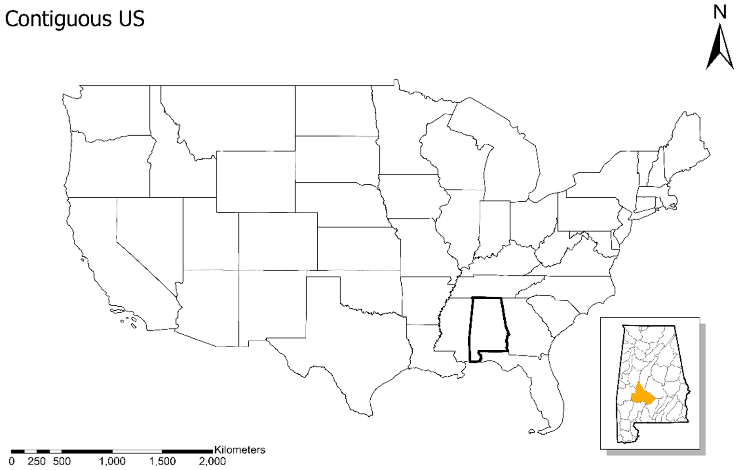
The project area (Middle Alabama Basin) is located in a warm temperate climate that is fully humid with hot summers (Figure 1).

The average annual precipitation is 1400 mm, with the maximum monthly value recorded in March at about 138 mm, and the minimum monthly value recorded in October at about 86.4 mm. The lowest minimum temperatures occur in December and January, with values between 1.7 and 2.2 °C. The highest maximum temperatures occur in July and August with values approaching 33 °C. Topography is generally characterized by gently rolling hills, sharp ridges, prairies, and alluvial flood plains. Elevation in the project area ranges from 100 to 1800 m. The watershed is sparsely developed (3%) and predominantly forest land (55%). The Middle Alabama watershed is sparsely populated with an estimated population of 148,000. This is a socially and economically disadvantaged region in Alabama with a population below the poverty rate of 27.3% as opposed to 15.5% statewide.

The Middle Alabama Watershed HUC 8 comprises 577,098 hectares, including 103,258 hectares of agricultural land. The agricultural land has 90,108 hectares not irrigated and 1009 hectares irrigated.

1.3. Soils

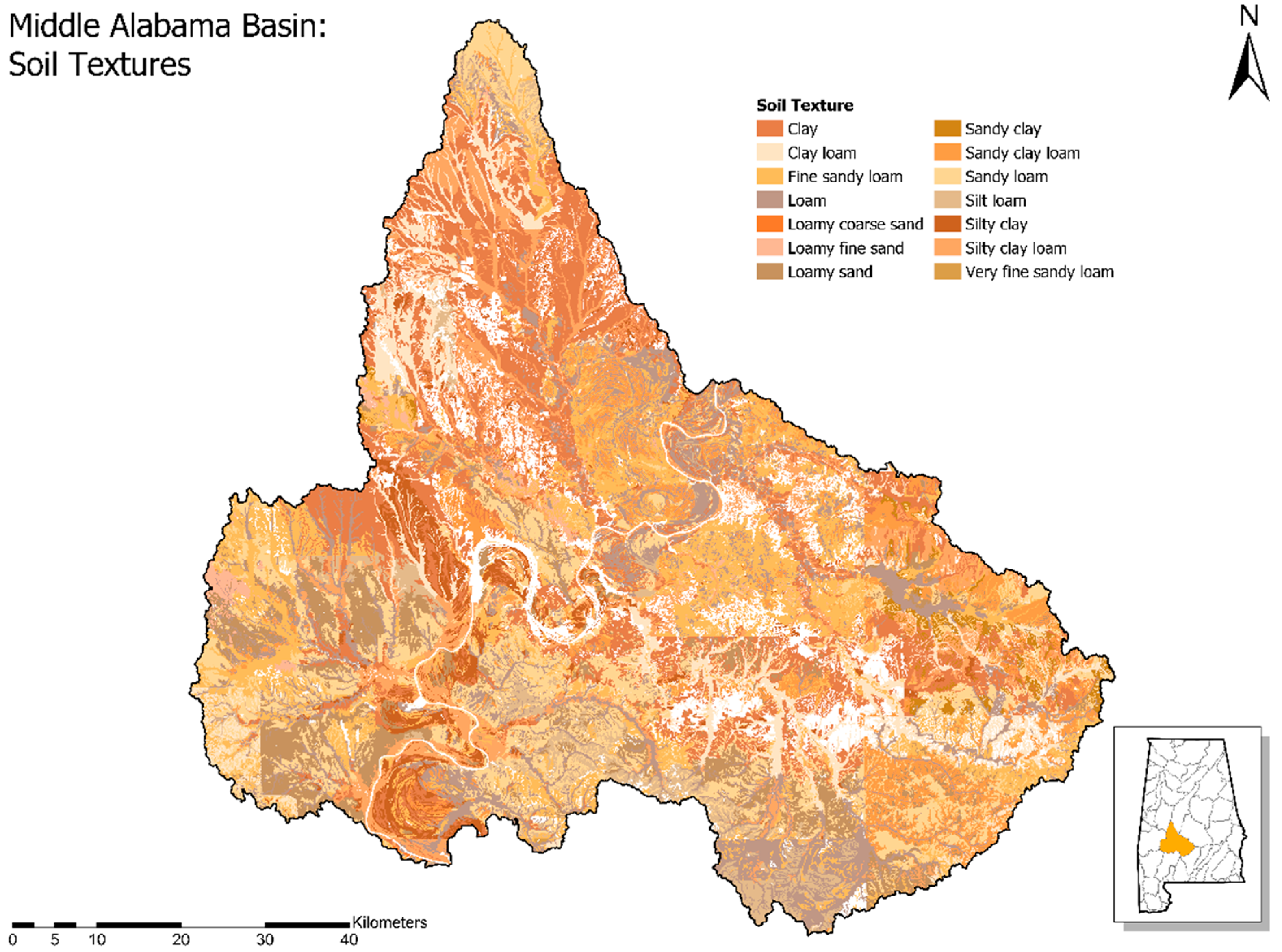
As shown in Figure 2 the soils of the basin are predominately clays, clay loams, silty clays, and silty clay loams. As a rule, these soils would be slow draining and therefore would produce relatively high runoff for given storm events.

Figure 3 displays the hydrologic soil groups HSG) of the basin. HSG classify soils as to drainage or infiltration capacity. The soil in the Middle Alabama Basin is generally composed of C and D hydrologic soil groups with 43% of the area being Group D and 29% Group C (Figure 3). The final 28% of the area in the Middle Alabama Basin consists of Groups A, B, B/D, and C/D. Group D soil primarily consists of clay soils that have high swelling potential, high runoff potential, and slow infiltration rates of less than 0.02 cm/h. Group C soils also tend to have slow infiltration rates between 0.02–0.05 cm/h. and moderate to high runoff potential [8].

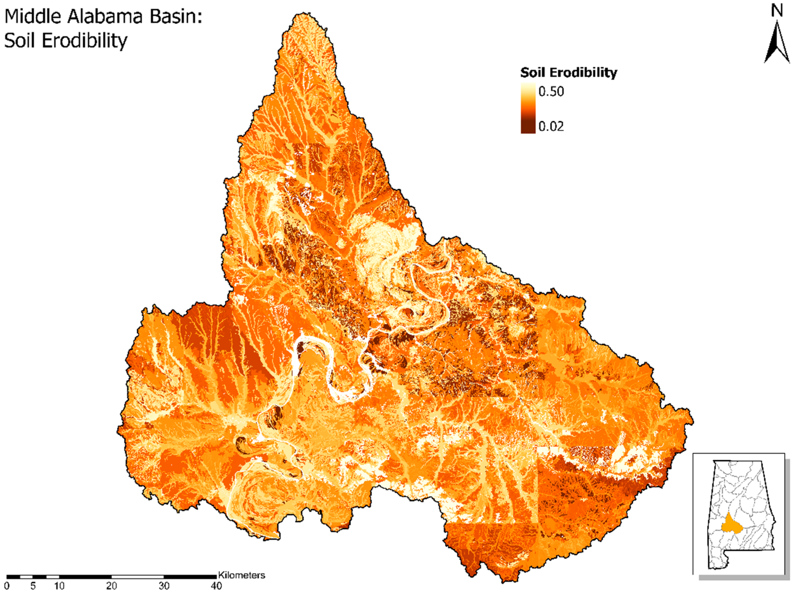
The spatial distribution of the soil erodibility index of the watershed is shown in Figure 4. The erodibility generally mimics the soil texture map with the higher erodibility soils located in the upper reaches of the basin.

1.4. Land Cover

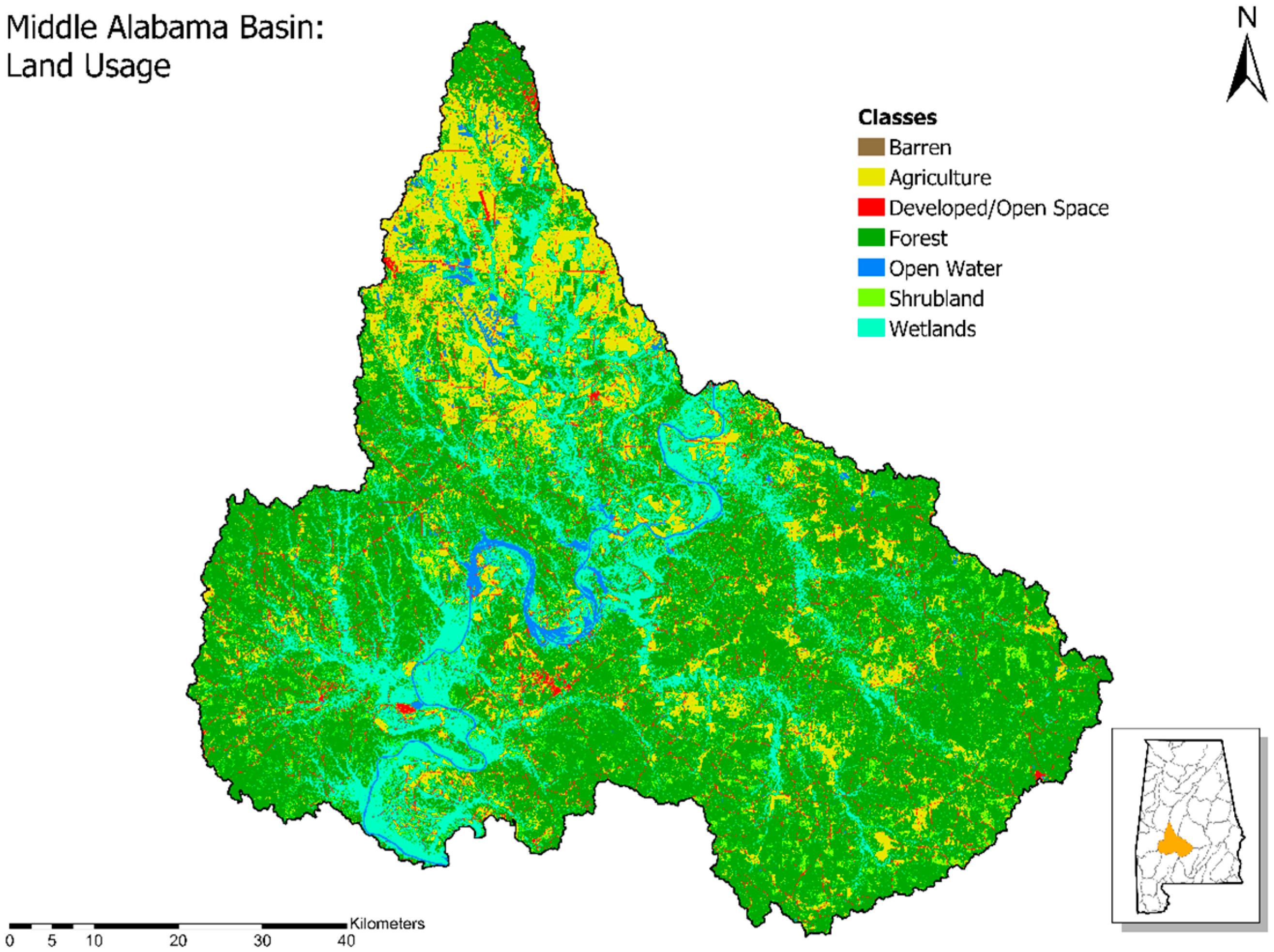
The land cover of the Middle Alabama Basin is predominantly forested with agricultural land generally located in the northern third of the basin (Figure 5). There is very little urban or developed land in the watershed. Other land cover classes in the watershed include wetlands (19%) and agriculture land (16%).

The topography of the basin is moderate with the steeper areas confined to the headwaters of the tributaries (Figure 6). There are many large floodplains with very little slope and then gently sloping planes above those. Since agricultural land is generally located on the more moderate slopes, or even in the flood plains, then the sediment export from the fields would be expected to be suppressed. Figure 4 shows that the soil erodibility is usually lower in these areas as well.

Based on an evaluation of the databases with respect to the goals and constraints of the federal irrigation program, and with the resources available, it was decided to concentrate on two ecosystem services: soil erosion and nutrient transport (water quality). Other potential services, such as increased crop yield (provisioning service) were not allowed to be considered under the program. In contrast to the Troy and Bagstad [6] procedure, ecosystem services were only evaluated for one land cover (agricultural) rather than all covers in the database. This was due to the nature of the overall project, which was just to evaluate the effects of expanded irrigation on existing agricultural land.

2. Materials and Methods

2.1. Materials

2.1.1. Soil Erosion: Universal Soil Loss Equation

One ecosystem service that is being evaluated in the study is soil loss from irrigated fields in the basin. In order to perform this analysis a version of the Universal Soil Loss Equation (USLE) developed by the US Agricultural Research Service is being employed. Soil loss calculated by the equation under irrigated conditions is compared to baseline (i.e., rain-fed) conditions without irrigation.

The USLE was developed during the 1950’s and 60’s by the Agricultural Research Service of the US Department of Agriculture [9]. It was felt at that time that a method needed to be developed to predict annual erosion losses from cultivated land in order to develop conservation measures to reduce soil losses in the US. The USLE resulted from this effort. The equation is empirical in nature and tries to relate erosion losses to weather, soil and land practice factors that would be expected to affect soil loss as follow:

A = R × K × LS × C × P

(1)

where, A = long term annual soil loss (tons/acre or tonnes/ha) for the subject area and R = energy factor for dislodging and transporting soil particles for the area where the subject field is located. The R-factor is theoretically calculated as a product of the kinetic energy of a rainfall event times its maximum 30-min intensity of fall. K = the soil erodibility factor, which corresponds to the collective effects of the detachment susceptibility of soil and the sediment transportability as well as the amount and rate of runoff under a given rainfall erosivity. LS = the slope length-gradient factor, which corrects the K value to account for the slope length and ground slope of the actual area of interest. C = crop management factor (dimensionless) and P = conservation practice factor (dimensionless).

While the USLE proved to be an effective tool for soil conservation studies, it was not thought to be ideal for the situation in this case. The principal reason is that there is no mechanism in the original USLE to account for changes in soil moisture between rainfed and irrigated conditions. The soil erodibility factor (k) accounts for soil texture and organic content, but not moisture content. However, due to some ambiguities with the rainfall energy factor (R), Williams [10] replaced the rainfall factor with a runoff energy factor to develop the Modified USLE (MUSLE) [9]. This substitution introduces the possibility of accounting for soil moisture variations. The equation was developed using individual storm data from 18 basins in Texas and Nebraska and subsequently validated on 102 basins throughout the United States using runoff data generated by the hydrologic component of the Simulator for Water Resources in Rural Basins (SWRRB) model [11].

2.1.2. The Modified Universal Soil Loss Equation

Is calculated as follows:

Y = CR × E × K × LS × C × P

(2)

where, Y = sediment yield for a particular runoff event (m tons), CR = conversion factor depending on units = 11.8 for SI units, E = erosivity energy factor for soil movement initiated by runoff, and the other factors are as before in the USLE.

The runoff energy factor is a function of both the volume of runoff for a particular event and its peak runoff rate:

$${\mathrm{E}=(\mathrm{Qq}}_{\mathrm{p}}{)}^{0.56}$$

(3)

where, Q = runoff (m³) and ${\mathrm{q}}_{\mathrm{p}}$ = peak runoff (m³/s).

The runoff, and to some extent the peak runoff, will be related to the antecedent soil moisture condition (AMC) before the rain event. The AMC can be introduced into the analysis through the use of the NRCS curve number [12]. The curve number (CN) was developed as a method to specify the total potential losses in a catchment with a specific land cover/soil matrix. The relationship between the total losses (S) and the CN is:

$$\mathrm{S}=\left(\frac{1000}{\mathrm{CN}}\right)-10$$

(4)

It is obvious that as the CN increases, the total potential losses decrease. Higher CN are associated with urban land covers and/or relatively impervious soils such as clays while lower CN appear under relatively undeveloped areas and highly pervious soils such as forests and sands. Cultivated land can exhibit fairly high CN depending on the soil classification.

For purposes of CN estimation, soils are classed into one of four hydrologic soil groups (HSG) based on drainage characteristics as shown in

Table 1. Hydrologic Soil Groups.

Class	Drainage Characteristics
A	Well drained, high infiltration rate, Sands
B	Moderately well drained, moderately high infiltration rate, silts, some sands
C	Moderately slow drained, slow infiltration rate, some clays
D	Poorly drained, very slow infiltration rate, clays

:

A search of the literature has revealed very little research into curve numbers associated with irrigated fields. Therefore, the impacts of irrigation on both sediment and nutrient exports were based on the results of experiments conducted on corn plots by Ellenburg [3] and further described by Ellenburg et al. [7]. The study area of these experiments was in the same region (North Alabama) with similar soil types and slopes as the Middle Alabama, so it is expected that the results will translate well. In these experiments, various fertilizer amounts, and delivery strategies were applied to corn plots under both rain-fed and irrigated conditions. A standard crop model, the Decision Support System for Agrotechnology (DSSAT), was used to model the crop growth, nitrogen usage and plant stress [13,14]. The DSSAT model accounts for the complete nitrogen cycle including mineralization, denitrification, crop uptake and soil leaching. However, it does not account for any lateral movement of water from the field due to runoff. In order to account for this, a kinematic wave-based model was developed by Ellenburg to carry surface runoff and mobilized residual nitrogen off the site.

The Ellenburg study encompassed two years—2010 and 2011. In general, 2010 could be considered a relatively dry year with about 700 mm of precipitation occurring during the growing season, while 2011 was wetter receiving about 900 mm of rain during the growing season. The runoff values for the two seasons were 94 mm and 149 mm for the rain-fed plots in 2010 and 2011, and 97 mm and 161 mm for the irrigated plots for the two years respectively. Thus, there was an increase of 3.2% in runoff between the rain-fed and irrigated fields in 2010 (dry year) and 8% increase in the wet year (2011). In order to be conservative, we assumed an 8% increase in runoff across the board between the rain-fed and irrigated conditions in the Middle Alabama watershed.

2.2. Methodology

2.2.1. Sediment Method

The climate station at Camden, Alabama was used to represent the climate conditions over the basin. The study is based on the last six years of the record (2017–2022) and only the rainfall during the growing season (June–August) was of interest to determine the impact of irrigation on the sediment yield from the agricultural region of the basin. The runoff was computed from the daily rainfall data using the NRCS curve number methodology:

$$\mathrm{Q}=\frac{{(\mathrm{P} - 0.2\mathrm{S})}^2}{(\mathrm{P}+0.8\mathrm{S})}$$

(5)

where, Q = runoff (mm) and P = daily precipitation (mm).

In Equation (5), the numerator term 0.2S represents the initial abstractions in the basin, i.e., interception, depression storage, etc. Therefore, for runoff to occur, the precipitation must exceed the initial abstractions.

First an evaluation of the land cover, soils, and topographic characteristics of the Middle Alabama watershed was performed. Based on the land cover map (Figure 5), the overwhelming majority of the agricultural land is in the northern part of the basin. Comparison with the soils map (Figure 3) it can be seen that the soils in this region are predominantly clay which would be classed as HSG D. Based on NRCS guidance [12] for row crop agriculture in good condition with some conservation overlaying class D soils leads to a CN of 86 (S = 1.62 cm). Based on the reasoning outlined above, this could be taken to represent rain fed conditions. For irrigated conditions, an increase of 8% from the base value was assumed based on the Ellenburg study [3].

The runoff energy factor (Equation (3)) is ${\mathrm{E} = (\mathrm{Qq}}_{\mathrm{p}}{)}^{0.56}$. In the computation of this factor NRCS methodology was followed as before. The peak runoff rate is given by a solution of the NRCS triangular unit hydrograph [15]:

$${\mathrm{T}}_{\mathrm{ov}}{=\mathrm{K}\left(\mathrm{NL}\right)}^{0.467}{\mathrm{S}}^{-0.235}$$

(6)

where, T_ov = overland flow travel time (min), K = 1.44 (SI units), N = overland flow retardance factor, L = plane length of overland flow (m) and S = plane slope (m/m).

Similarly, the channel flow time is computed from the well-known Kirpich Equation:

T_ch = K_ch L_ch^0.77 S_ch^−0.385

(7)

where, T_ch = channel travel time in min, K_ch = 0.0195 (SI units) and L and S are channel length and slope as before. The computations were done for a representative one square mile area of the Middle Alabama watershed, i.e., the flow course length is 2126 m, the mean land slope is 1.7% and CN is given above. It can be noted that the computations of runoff (Q) and peak runoff rate (${\mathrm{q}}_{\mathrm{p}}$) are in English units while the MUSLE computations are in SI units. In this case, the NRCS computations were done as above and then the runoff and peak values were converted to SI units.

2.2.2. MUSLE Parameters of Rain-Fed vs. Irrigation Conditions

Baseline conditions were estimated to evaluate the impact of the expansion of sustainable irrigation practices on sediment yields. The baseline factors for C and P were derived from a biophysical table developed in TerrSet 2020 (v.19.0.6) linking agriculture conservation, practices and other biophysical factors with land cover land use classes (see Supplementary Materials). The K factor for the watershed is from the Soil Survey Geographic Database (SSURGO) soils data. The soil erodibility factor was calculated by averaging erodibility values from the Esri USA SSURGO Erodibility Factor Living Atlas across each basin [16]. The average erodibility of 0.24 in the Middle Alabama Basin was applied in the MUSLE.

Other factors were adjusted to estimate the effect of project implementation based on assumed sustainable conservation and farming practices (factors C and P). Potentially the use of conservation practices such as no till agriculture, contour farming, and crop rotations could reduce sediment loads and improve water quality. Based on the implementation of more sustainable agricultural practices with irrigation on all the agricultural land; we assume spring conservation, including crop rotations and no till agriculture to adjust the C factor to 0.24 [8]. While contour farming in slope areas would potentially merit an adjustment of the P factor, however, the Middle Alabama is relatively flat, so no conservation adjustment was made. The following values of the relevant factors were used in the baseline analysis:

• Mean K (soil erodibility) = 0.24; average from the SSURGO soils data
• C (cover management) = 0.37; average from the biophysical table, only agriculture land. (See Supplementary Materials)
• P (conservation practice) = 0.5; average from the biophysical table, only agriculture land. (See Supplementary Materials)
• LS (slope steepness and length) = 0.50; The slope length (L) for the Middle Alabama Basin was obtained by measuring the distance over agricultural land between five sets of points throughout the Basin. The lengths of all 10 sets of points were averaged for a value of 83.2 m (2733 ft). The slope steepness factor (S) was calculated by estimating the slope for all five sets of points and were averaged to obtain a percent slope of 1.69. The overall LS value of approximately 0.5 was derived from a biophysical table in Ward et al. (see Supplementary Materials) using slope length and percent slope.

For the irrigation model simulations, all factors remain the same except for the cover management factor C. Cover management was modified to assume conservation tillage and reduced to a C factor of 0.24 for the irrigated case. An evaluation of census data for row crops in Perry and Dallas counties, which represent a large majority of the agricultural land in the Middle Alabama basin, indicates that about 60% of the row crop farmers are using no till or reduced tillage in their fields [17]. Therefore, the results of the rainfed (RF) simulation are a combination of 60% yield calculated using the conservative C (0.24) and 40% yield using the C = 0.37. This is our baseline or current conditions. For expanded irrigation (IR) on existing agricultural land, we assume no till or reduced tillage on all new agricultural land irrigated (C = 0.24). The combined scenario (CB) assumes we realistically add approximately 20% irrigated acreage to the mix, so the results are calculated as follows:

$$\mathrm{Y}=\left(\mathrm{RF} \times 0.8\right)+(\mathrm{IR} \times 0.2)$$

(8)

The MUSLE estimates the soil loss for each runoff event in terms of the amount of soil that was moved. This needs to be distinguished from the amount that actually reaches the hydrologic system. This load is a proxy for the estimated ecosystem services, positive or negative, that will result from row crop farming practices under rainfed and irrigated scenarios. As such, average soil delivery ratios for drainage areas for various sizes have been developed [18]. A delivery ratio of a representative square mile for the Middle Alabama is 3 percent of the total sediment load moved. Thus, to estimate the total sediment loss to the system, and the associated positive or negative ecosystem services, the results from MUSLE are multiplied by 0.03.

2.2.3. Valuation of Sediment Reduction

The ecosystem service for sediment reduction is valued as the cost of removing deposited sediment from waterways, which is avoided by this project. An assumed economic value of sediment volume removed is taken from Cooke et al. [19] at $8 per cubic meter, in 2021-dollars after adjusting for inflation.

2.2.4. Nutrient Method

Our method estimates Total Nitrogen runoff from agricultural fields under rainfed and irrigation scenarios. Total Nitrogen (TN) is composed of nitrates, nitrites, organic nitrogen and ammonia. Nitrite and ammonia compounds are usually present in low quantities unless the waterway is heavily polluted and are not considered in our analysis. Agriculture and wastewater are primary sources, however, we are only focused on TN from agricultural fields. Increased nitrogen levels can cause algae blooms and decrease dissolved oxygen leading to fish kills and overall degradation of the aquatic habitat [20]. As in the previous case, the baseline runoff was calculated for rain-fed conditions using a CN of 86. Then, as before, these values were increased by 8% to represent irrigated conditions.

The same concept was employed to calculate the nutrient runoff as in the case of sediment runoff. The Ellenburg experimental data are given in

Table 2. Experimental Data in North Alabama on Nitrogen Export for Corn Crops.

Year	P (mm)	Q-RF (mm)	Q-Irr (mm)	N-RF (kg/ha)	N-Irr (kg/ha)
2010	699	94.23	97.34	45.3	39.5
2011	901	149.28	161.58	33.36	41.68

below:

The percent difference between rain-fed and irrigated nutrient export per mm of runoff was applied to the runoff values computed for the Middle Alabama basin. These ratios are 0.48 kg/ha/mm for 2010 rain-fed; 0.40 kg/ha/mm for 2010 irrigated; 0.22 kg/ha/mm for 2011 rain-fed and 0.26 kg/ha/mm for 2011 irrigated. Applying these ratios to the runoff values (increasing the base rain-fed values by 8% as before), the nutrient exports were computed for both rain-fed and irrigated conditions.

The landscape delivery ratio (LDR) parses the fertilizer load in runoff that, due to soils and landscape characteristics, reaches the stream channel [21]. An LDR of 0.30 is assumed for the Middle Alabama watershed, which accounts for the nutrient losses during overland flow from the field to the stream. Fertilizer loads for rainfed agricultural land are estimated at 140 kg/ha and for irrigated fields 280 kg/ha [22,23]. The ecosystem services value of nutrient reduction is measured as the societal cost of nitrogen loss to waterways and is valued at $1.76 per kg, in 2021-dollars after adjusting for inflation [24]. This value is obtained as the equilibrium price from a nutrient trading scheme in Chesapeake Bay.

3. Results

3.1. Sediment Loads & Ecosystem Services

The simulation results for sediment loads in both rain-fed and irrigated conditions are summarized in

Table 3. Climate and Runoff Data with Resulting Sediment Loads and Associated Ecosystem Services.

Year	No. Events	P (mm)	Qir (mm)	Qrf (mm)	YRF	YRF+IR	Diff (Tonnes/ha)	ES Value ($/m3/ha)
2017	26	544.32	164.59	152.40	8.0	7.83	−0.17	−0.11
2018	25	423.7	101.53	94.01	4.67	4.57	−0.10	−0.06
2019	19	317.5	61.04	56.52	2.67	2.61	−0.06	−0.04
2020	16	316.48	64.20	59.44	2.73	2.67	−0.06	−0.04
2021	28	521.72	145.02	134.28	6.97	6.82	−0.15	−0.10
2022	19	423.42	182.10	182.10	9.47	9.28	−0.20	−0.13

below. For each year, the simulated results for each individual runoff event are summed to get the annual value and associated ecosystem service benefit (+) or cost (−).

The results indicate that, under the conditions assumed in this analysis, the irrigated fields export slightly less sediment than do the rain-fed fields. The additional conservation measures assumed in the irrigated scenario largely offsets the increased runoff and sediment from irrigated versus rainfed fields as noted in the low annual ecosystem service costs.

However, the results also show the impact of climate on sediment yield. Not surprisingly, the wetter years tended to produce the most sediment yield since they also produced the most surface runoff. However, the MUSLE equation indicates that, with proper conservation measures applied, increased sediment discharge from irrigated fields can be mitigated.

3.2. Nutrient Loads & Ecosystem Services

The results from the nutrient export analysis are given in

Table 4. Climate Data with Nutrient Loads and Associated Ecosystem Services.

Year	No. Events	P (mm)	Nrf (kg/ha)	Nir (kg/ha)	Diff (kg/ha)	ES Value ($/kg/ha)
2017 (wet)	26	544.32	33.28	40.73	−7.45	−3.93
2018 (wet)	25	423.7	20.53	25.13	−4.59	−2.42
2019 (dry)	19	317.5	26.59	22.89	+3.69	+1.95
2020 (dry)	16	316.48	27.96	24.07	+3.88	+2.05
2021 (wet)	28	521.72	29.32	35.89	−6.56	−3.46
2022 (wet)	19	423.42	36.82	45.07	−8.24	−4.35

below:

The nutrient export results are in general agreement with the results of past investigations described in the literature [25,26,27,28]. As in the sediment case, climate plays an important role in nutrient export. As seen in the results, during the two dry years (2019, 2020) the irrigated fields exported less nitrogen than did the rain-fed fields while the reverse was true of the wetter years. This phenomenon is related to the uptake efficiency of the corn plants under wet and dry conditions. When conditions in the field are dry, there is not enough moisture available for the plants to uptake all of the nutrients that they need. Thus, the residual nitrogen left in the soil is available for transport when rain events do occur. In general, droughts have been associated with an increase in the nitrogen left in the soil [29,30]. On the other hand, wet (or irrigated) conditions mitigate this situation by “watering in” the nitrogen into the soil column for easy uptake by the plants.

Ecosystem service values correlate with the nitrogen export values show that positive ecosystem service benefits exist during dry years when irrigation is more likely to be needed to sustain crops. However, the differences in ecosystem service benefits or costs are small between the dry and wet years. As an illustration, the AIP plans to irrigate about 405 hectares of existing agricultural land in the Middle Alabama basin over the next year. If we assume 2019 values for the dry year and 2021 values for the wet year since each of these years have the most events, the annual ecosystem service benefit from the AIP in 2019 is $790.00 and the ecosystem service cost in 2021 is −$1402.

4. Discussion

Both the sediment and nutrient methods used to estimate the respective loads entering the hydrologic system plus valuation approaches are based on established literature and experimental results. The valuation approaches are variable and may be affected by regional and local economics. The benefits from being able to quantify ecosystem services with established methods are substantial. For example, the value (plus or minus) of ecosystem services can be included in benefit/cost analyses that are used to make multiple decisions regarding how development affects the natural environment and whether or not to proceed with various types of development projects. Resource managers and other decision-makers have to make difficult decisions on a daily basis and more robust data, numbers versus qualitative assessments, are essential to help them make best possible decisions for the benefit of society.

While our analysis and results are most closely aligned with regulating and supporting ecosystem services for improved water quality that results from reduced nutrient and sediment loads discharged into streams and rivers, our methods are not robust enough to parse benefits discretely among each ecosystem service type. Arguments may also be made that improved water quality will provide some cultural and provisioning ecosystem service benefits too. Being able to parse benefits by ecosystem service type is a major challenge that will require new methods to be conceptualized along with additional variables and assumptions.

We believe the methods presented herein are transferable to other similar agricultural (corn crops) and climatic regions in the southeast US with minor adjustments to the factors used in the MUSLE and adjustments based on experimental results. Most (if not all) states have Land Grant schools with agricultural extension services that conduct the type of experiments used in this study. However, there are challenges in using the methods in different climate and crop type regions, including using data from different sources and difficulty in acquiring all the data needed. While soils data are available nationally, climate data varies by region and data from NRCS, or agricultural extension services is of varying availability and quality in some areas.

To illustrate some of these issues, we explored application of the sediment and nutrient methods to the Central Valley of California. Data gathered from the Upper Dry watershed in the Central Valley of California showed different climate, farming techniques, and land use than the Middle Alabama watershed. The Upper Dry watershed land cover land use is primarily agriculture, however, grassland/pasture (16%), developed land in the Fresno metropolitan area (11%) and forest (4%) land are also found. The forest land is largely found in the upland areas east of Fresno, California toward the Sierra National Forest and upland areas at the western end of the watershed toward the Pacific Coast Mountain ranges. While the Upper Dry does get an average annual rainfall of approximately 254 mm, this is about five times less than in Alabama where the average annual rainfall is 1400 mm. Irrigated land in the Upper Dry is approximately 393,588 hectares while the Middle Alabama is only 1019 hectares [30,31]. Out of total cropland, this means that 85% of cropland in the Upper Dry is irrigated while only 1.2% of cropland is irrigated in the Middle Alabama. Agricultural land use is also vastly different. Both watersheds are similar in size (Upper Dry with 550,630 hectares and Middle Alabama with 577,098 hectares) but the percent of crop to land use and diversity of crops is significantly higher in the Upper Dry compared to Middle Alabama. There are around 13 different types of crop groups grown in the Upper Dry with fruit trees and fruit using up a2proximately 37% of crop land while the Middle Alabama has around 10 different crop groups with fallow/idle cropland and grains using approximately 13% of crop land [32]. All of these factors combined make it very difficult for a 1-to-1 comparison. Given the crop diversity, climate and soil moisture differences, determining the appropriate fertilizer loads, landscape delivery ratios to streams and appropriate cover crop (C factor) and farming practices (P factor) would be unique challenges compared to the southeast US.

5. Conclusions

An approach to quantify ecosystem service values provides complementary added value to only qualitative information. Being able to quantify the value of ecosystem services allows these services to be included in benefit/cost ratios and provide resource managers with stronger data to support decision-making. The data required for the sediment and nutrient approaches is readily available and the methods are readily transferable to other watersheds in the southeast with similar crops and farming practices. Using the method outside the southeast US in regions with different crops, climates, and farming practices will require more research to establish appropriate input values.

References

- Carter, L.; Terando, A.; Dow, K.; Hiers, K.; Kunkel, K.E.; Lascurain, A.; Marcy, D.; Osland, M.; Schramm, P. Southeast. Impacts, Risks, and Adaptation in the United States. In Fourth National Climate Assessment; Reidmiller, D.R., Avery, C.W., Easterling, D.R., Kunkel, K.E., Lewis, K.L.M., Maycock, T.K., Stewart, B.C., Eds.; U.S. Global Change Research Program: Washington, DC, USA, 2018; Volume II, pp. 743–808. [Google Scholar] [CrossRef]
- Rosa, L.; Chiarelli, D.D.; Sangiorgio, M.; Beltran-Peña, A.A.; Rulli, M.C.; D’Odorico, M.C.; Fung, I. Potential for sustainable irrigation expansion in a 3 °C warmer climate. Proc. Natl. Acad. Sci. USA 2020, 117, 29526–29534. [Google Scholar] [CrossRef] [PubMed]
- Ellenburg, W.L. The Impact of Irrigation on Nutrient Export from Agricultural Fields. Master’s Thesis, University of Alabama in Huntsville, Huntsville, AL, USA, 2011. [Google Scholar]
- Millennium Ecosystem Assessment. Ecosystems and Human Well-Being: Synthesis; Island Press: Washington, DC, USA, 2005. [Google Scholar]
- National Wildlife Federation, Ecosystem Services. Available online: https://www.nwf.org/Educational-Resources/Wildlife-Guide/Understanding-Conservation/Ecosystem-Services (accessed on 2 October 2022).
- Troy, A.; Bagstad, K. Estimation of Ecosystem Service Values for Southern Ontario; Spatial Informatics Group, LLC: Pleasanton, CA, USA, 2009. [Google Scholar]
- Ellenburg, W.L.; Cruise, J.F.; Ortiz, B.V.; Suhs, R. The impact of irrigation on surface nitrate export from agricultural fields in the Southeastern US. J. Environ. Qual. 2022; under review. [Google Scholar]
- Ward, A.; Trimble, S.; Burckhard, S.; Lyon, J. Environmental Hydrology, 3rd ed.; CRC Press, Taylor and Francis Group: Boca Raton, FL, USA, 2016; ISBN 13: 978-1-4665-8941-4. [Google Scholar]
- Wischmeier, W.H.; Smith, D.D. Predicting Rainfall Erosion Losses. A Guide to Conservation Planning; The USDA Agricultural Handbook No. 537; USDA: Beltsville, MD, USA, 1978. [Google Scholar]
- Williams, J.R. Sediment-yield prediction with Universal Equation using runoff energy factor. In Present and Prospective Technology for Predicting Sediment Yield and Sources; ARS-S-40; USDA: Washington, DC, USA, 1975; pp. 244–252. [Google Scholar]
- Williams, J.R. Testing the Modified Universal Soil Loss Equation. In Proceedings of the Workshop on Estimating Erosion and Sediment Yield on Rangelands, Tucson, AZ, USA, 7–9 March 1981; ARM-W-26. Agricultural Research Service: Oakland, CA, USA, 1982; pp. 157–161. [Google Scholar]
- U.S. Department of Agriculture; Natural Resources Conservation Service. Time of concentration. In National Engineering Handbook; Part 630; U.S. Department of Agriculture: Washington, DC, USA, 1972; Chapter 15. [Google Scholar]
- Jones, J.; Hoogenboom, G.; Porter, C.H.; Boote, K.J.; Batchelor, W.D.; Hunt, L.A.; Wilkens, P.W.; Singh, U.; Gijsman, A.J.; Ritchie, J.T. The DSSAT cropping system model. Eur. J. Agron. 2003, 18, 235–265. [Google Scholar] [CrossRef]
- Hoogenboom, G. Decision Support System for Agrotechnology Transfer (DSSAT). 2010. Available online: www.dssat.net (accessed on 7 July 2022).
- Pongsai, S.; Schmidt, V.; Shrestha, R.P.; Clemente, R.S.; Eiumnoh, A. Calibration and validation of the Modified Universal Soil Loss Equation for estimating sediment yield on sloping plots: A case study in Khun Satan catchment of Northern Thailand. Can. J. Soil Sci. 2010, 90, 585–596. [Google Scholar] [CrossRef] [Green Version]
- The Gridded Soil Survey Geographic (gSSURGO) Database for Alabama. United States Department of Agriculture, Natural Resources Conservation Service. Available online: https://gdg.sc.egov.usda.gov/FY2015officialrelease (accessed on 29 August 2022).
- Perdue, S.; Hamer, H. 2017 Census of Agriculture: Alabama State and County Data; AC-17-A-1; United States Department of Agriculture’s National Agricultural Statistics Service: Annapolis, MD, USA, 2019; pp. 51–555. [Google Scholar]
- Roehl, J.N. Sediment Source Areas, Delivery Ratios and Influencing Morphological Factors. Intern. Assoc. Sci. Hydrol. 1962, 59, 202–213. [Google Scholar]
- Cooke, G.D.; Welch, E.B.; Peterson, S.A.; Nichols, S.A. Restoration and Management of Lakes and Reservoirs, 3rd ed.; CRC Press: Boca Raton, FL, USA, 2005. [Google Scholar]
- U.S. EPA (United States Environmental Protection Agency). National Estuary Program—Challenges Facing Our Estuaries. Key Management Issues: Nutrient Overloading. 2005. Available online: https://www.epa.gov/nep/how-national-estuary-programs-address-environmental-issues (accessed on 8 August 2022).
- Hoos, A.B.; McMahon, G. Spatial analysis of instream nitrogen loads and factors controlling nitrogen delivery to streams in the southeastern United States using spatially referenced regression on watershed attributes (SPARROW) and regional classification frameworks. Hydrol. Process. 2009, 23, 2275–2294. [Google Scholar] [CrossRef]
- Patterson, P. Crop, Soil and Environmental Sciences Departmental Series Alabama Agricultural Experiment Station, Auburn University. 2020. Available online: https://aurora.auburn.edu/bitstream/handle/11200/49810/AlabamaRowCropsPDF_R2_AGedits.pdf?sequence=1&isAllowed=y (accessed on 1 September 2022).
- Debaeke, P.; Hilaire, A. Production of rainfed and irrigated crops under different crop rotations and input levels in southwestern France. Can. J. Plant Sci. 1997, 539–548. Available online: https://cdnsciencepub.com/doi/pdf/10.4141/P96-089 (accessed on 15 October 2022).
- Ribaudo, M.; Savage, J.; Aillery, M. An Economic Assessment of Policy Options to Reduce Agricultural Pollutants in the Chesapeake Bay; ERR-166; United States Department of Agriculture, Economic Research Service: Annapolis, MD, USA, 2014. [Google Scholar]
- Liang, B.C.; Remillard, M.; MacKenzie, A.F. Influence of Fertilizer, Irrigation, and Non-Growing Season Precipitation on Soil Nitrate-Nitrogen under Corn. J. Environ. Qual. 1991, 20, 123. [Google Scholar] [CrossRef]
- Allaire-Leung, S.E.; Wu, L.; Mitchell, J.P.; Sanden, B.L. Nitrate leaching and soil nitrate content as affected by irrigation uniformity in a carrot field. Agric. Water Manag. 2001, 48, 37–50. [Google Scholar] [CrossRef]
- Merchán, D.; Causapé, J.; Abrahao, R. Impact of irrigation implementation on hydrology and water quality in a small agricultural basin in Spain. Hydrol. Sci. J. 2013, 58, 1400–1413. [Google Scholar] [CrossRef] [Green Version]
- Phene, C.J.; Beale, O.W. High-frequency Irrigation for Water Nutrient Management in Humid Regions1. Soil Sci. Soc. Am. J. 1976, 40, 430. [Google Scholar] [CrossRef]
- Nafziger, E.; Spring Soil Nitrogen Following the Drought of 2012. In The Bulletin: Integrated Pest and Crop Development; 2013. Available online: https://farmdoc.illinois.edu/field-crop-production/crop_production/spring-soil-nitrogen-following-the-drought-of-2012.html (accessed on 15 August 2022).
- NRCS. Drought Increases the Risk of Soil Erosion and Nitrogen Leaching, Huron, S.D. 2012. Available online: http://articles.aberdeennews.com/2012-10-19/farmforum/34592139_1_drought-increases-nitrate-n-drought-conditions (accessed on 28 September 2022).
- USDA. Guidance for Conducting Analysis Under the Principles, Requirements, and Guidelines for Water and Land Related Resources Implementation Studies and Federal Water and Resource Investments; DM 9500-013; USDA: Annapolis, MD, USA, 2017. [Google Scholar]
- USDA. National Agricultural Statistics Service Cropland Data Layer; USDA-NASS: Washington, DC, USA, 2017. Available online: https://nassgeodata.gmu.edu/CropScape/ (accessed on 7 September 2022).