Article

Estimation and Dynamic Analysis of Soil Salinity Based on UAV and Sentinel-2A Multispectral Imagery in the Coastal Area, China

1
School of Geographical Sciences and Surveying Engineering, China University of Mining and Technology, Beijing 100083, China
2
School of Resources and Environment, Shandong Agricultural University, Taian 271018, China
3
School of Environment Science and Spatial Informatics, China University of Mining and Technology, Xuzhou 221116, China
*
Author to whom correspondence should be addressed.
Land 2022, 11(12), 2307; https://doi.org/10.3390/land11122307
Submission received: 25 October 2022 / Revised: 25 November 2022 / Accepted: 7 December 2022 / Published: 15 December 2022

Abstract

:
An efficient, convenient, and accurate method for monitoring the distribution characteristics of soil salinity is required to effectively control the damage of saline soil to the land environment and maintain a virtuous cycle of the ecological environment. There are still problems with single-monitoring data that cannot meet the requirements of different regional scales and accuracy, including inconsistent band reflectance between multi-source sensor data. This article proposes a monitoring method based on the multi-source data fusion of unmanned aerial vehicle (UAV) multispectral remote sensing, Sentinel-2A satellite remote sensing, and ground-measured salinity data. The research area and two experimental fields were located in the Yellow River Delta (YRD). The results show that the back-propagation neural network model (BPNN) in the comprehensive estimation model is the best prediction model for soil salinity (modeling accuracy R2 reaches 0.769, verification accuracy R2 reaches 0.774). There is a strong correlation between the satellite and UAV imagery, while the Sentinel-2A imagery after reflectivity correction has a superior estimation effect. In addition, the results of dynamic analysis show that the area of non-saline soil and mild-saline soil decreased, while the area of moderately and heavily saline soils and solonchak increased. Additionally, the average area share of different classes of saline soils distributed over the land use types varied in order, from unused land > grassland > forest land > arable land, where the area share of severe-saline soil distributed on unused land changed the most (89.142%). In this study, the results of estimation are close to the true values, which supports the feasibility of the multi-source data fusion method of UAV remote sensing satellite ground measurements. It not only achieves the estimation of soil salinity and monitoring of change patterns at different scales, but also achieve high accuracy of soil salinity prediction in ascending scale regions. It provides a theoretical scientific basis for the remediation of soil salinization, land use, and environmental protection policies in coastal areas.

1. Introduction

As an ecological problem, soil salinization has long been paid close attention to by governments and researchers worldwide. The Yellow River Delta (YRD) region has a shallow groundwater level, high salinity, and easy accumulation of groundwater salinity on the surface. Under different driving forces such as seawater intrusion, climate change, and human farming, its surface morphology and ecological environment have undergone dramatic changes [1,2]. Soil salinization has gradually become a major soil degradation and development problem facing the YRD in China, one that seriously restricts local agricultural productivity and food security [3,4]. Therefore, it is necessary to conduct re-al-time and accurate monitoring of soil salinization and its temporal and spatial dynamic changes in the YRD, which also prevents the deterioration of salinization, improves the ecological environment, and strengthens land management [5,6].
Traditional soil salinity measurement methods are accurate but time-consuming and labor-intensive [7,8], which is not conducive to monitoring soil salinity in large-scale areas. The rapid development of remote sensing technology since the 1990s has provided new ideas and methods for quantitative monitoring of soil salinity. Satellite remote sensing, such as Landsat, High Resolution, SPOT, and Sentinel, has been widely used in the quantitative estimation of soil salinity due to its large-scale and high-efficiency advantages [9]. UAV remote sensing technology realizes intelligent and rapid acquisition, processing, and analysis of high-resolution imagery data using GPS differential positioning technology, telemetry, remote control technology, and remote sensing technology [10,11,12,13,14]. A proximal sensing method, such as EM (Effective Microorganisms), has been widely used to monitor soil salinity globally. In particular, the quasi-3D joint-inversion between multiple sources of data provides additional more accurate and efficient methods for mapping soil salinity [15,16]. Although researchers have extensively researched the comprehensive application of multi-source data for saline soil monitoring and have achieved considerable results [17,18], most data sources are a combination of optical data and radar data, including the two different satellite remote sensing data methods. However, it is relatively lacking in the combination of satellite remote sensing, UAV remote sensing, and ground soil salinity measurement data.
The necessary premise for the reasonable prevention and control of soil salinization is to quickly and accurately obtain the spatial and temporal distribution of saline soil [19,20]. Scholars at home and abroad have performed the transformation and screening of different spectral parameters and related indices based on sensitive bands [20,21,22]. Based on the spectral characteristics of soil salinity, a large number of salinity indices such as Salinity Index 1-Salinity Index 6 (SI1-SI6) and the normalized difference salinity index (NDSI) have been established [7,23,24]. The research concluded that the recognition effect of the integrated band (covering the visible-near-infrared band and the combined band in the infrared spectral range) is superior to that of the independent band, and most of the vegetation index can be used as an estimation index of soil salinity content to reflect soil salinity indirectly [25,26]. In addition, linear regression methods such as support vector machines (SVM), partial least squares regression (PLSR), and machine learning methods such as backpropagation neural network (BPNN) and random forest (RF) are used in quantitative estimation and the estimation of soil salinity results [21,27,28,29,30]. Many combined, transformative, and innovative research methods have emerged for improving the accuracy of saline soil quantitative estimation using different remote sensing data sources for saline soils from varied regions [21,27,31,32,33]. However, the soil salinity sensitivity of different indices has strong regionality. In previous studies, the methods of spectral parameter selection and comparison of soil salinity estimation models were relatively common and single. A variety of modeling methods lack the sensitivity to verify the soil salinity with different band index combinations.
The study of the dynamic changes of soil salinization is a crucial and basic work for exploring the regional soil salinity variation pattern and formulating salinization management measures [34,35]. Land use types that change with time are unstable feature types. The stability of saline soils changes with land use type migration [36], as reflected in the dynamic changes of area of different grades of saline soils and the grade transformation between different grades of saline soils. Therefore, to further explore the stability and variability trends of different degrees of saline soils, it is necessary to analyze soil salinity dynamics in conjunction with land use types [37,38,39].
In this study, the following issues are discussed. (1) Construction of a soil salinity prediction model in the YRD based on UAV multispectral remote sensing imagery. (2) Reflectance of UAV multispectral imagery and Sentinel-2A satellite imagery correction. (3) Verification and estimation of the best prediction model for soil salinity in the experimental and study areas. (4) Analysis of the dynamics of saline soils in the YRD and their relationship with different land use types. A quantitative estimation of soil salinity is used to achieve different scales in different years in the YRD region.

2. Materials and Methods

2.1. Study Area

The study area is located in four counties, Hekou, Kenli, Dongying, and Lijin, of Dongying City, Shandong Province (37°16′–38°00′ N, 118°06′–119°18′ E), covering an area of approximately 6000 km2 (Figure 1). The region has a warm temperate continental monsoon climate, with cold winters, hot summers, and four distinct seasons. The annual average temperature is 13.23 °C, the average annual rainfall is 530 mm, and the average annual potential evaporation is 1500 mm [40]. The overall topography of the area tends to be flat, with the topography decreasing from southwest to northeast, and the average elevation is less than 15 m. Geomorphological types include granite, gentle hills, and shallow depressions. The study area is on the typical Yellow River alluvial plain in the YRD. The main soil types are fluvisol and solonchak, and the texture of the cultivated layer is most widely distributed with sandy loam and light loam, with an area proportion of over 70%. The test areas were two test fields located in Lijin County and the Kenli District. The salinity of the saline soil in the test area covers both high and low values, which are representative to a certain extent. A sampling point distribution diagram of the test areas is shown in Figure 1.

2.2. Data Acquisition and Preprocessing

The data acquisition and pre-processing in this study focused on soil salinity data, UAV image data, Sentinel-2A image data, and land use data. The methodological scheme of this study is shown in Figure 2.

2.2.1. Soil Salinity Data

Field investigations and soil sample collection were conducted from March 25 to 28, 2019. We conducted field research and field evidence beforehand, and clarified the approximate distribution of soils with high, medium, and low salinity in the study area based on the relevant results of the research. The bare soil area (containing only some crop straw) and the bare soil–crop mixed area were selected as the test areas, following the principle of covering the high and low values of soil salinity in the test area as much as possible by laid-out sample points according to a few meters x a few meters. A total of 129 sampling points and 36 calibration control points were arranged evenly in the interior. A handheld GPS locator was used to measure the field latitude and longitude coordinates of each sampling point. At the same time, environmental information such as topography, elevation, and vegetation type of the sampling sites were also recorded. A five-point sampling method was used to collect 0–20 cm surface soil samples at each sampling point. The obtained soil samples were cleaned of roots, stones, and other debris, fully mixed, naturally air-dried, ground, and sieved. The soil conductivity value was measured with a DDS-307A conductivity meter, with 30 extracts randomly selected. The corresponding total soil salt content was calculated and the conversion relationship between the soil salt content in the study area and the conductivity value of the extract was obtained (Equation (1)):
S t = 2.9863 E C 1 : 5 0.1019   R 2   =   0.9813   * *
where ** is the significance level at p < 0.01, S t is the total soil salt content (g·kg−1), and E C 1 : 5 is the conductivity of the 1:5 soil–water ratio of the soil extract (mS·cm−1), with the total salt content of the remaining soil samples without ion composition determination calculated from E C 1 : 5 using Equation (1). Three replicate experiments were performed for each treatment.

2.2.2. UAV Multispectral Imagery Data

The remote sensing platform used for imagery acquisition was the Matrice 600 Pro® six-rotor UAV produced by Shenzhen DJI Innovation Technology Co., Ltd., Shenzhen, China (the flight load is 5.5 kg, the hovering time is 16 min, and the maximum horizontal flight speed in a windless environment is 65 km·h−1), equipped with a Parrot Sequoia agricultural multispectral camera (containing four 1.2 million pixel narrow-band and synchronized monochromatic sensors, including four bands named Bg, Br, Breg, and Bnir) for near-ground imagery of UAVs in the test area. The acquisition time of the data was from 12:00 to 15:00 on 27 March 2019 (the weather was clear). The calibration control point (whiteboard) data were collected before takeoff, the flight height of the UAV was set to 50 m, the spatial resolution was 2.2 cm, the camera shooting time interval was 1.5 s, and three flight missions were performed.
In the later stage, Pixel Wrench2 software was used to extract, register, and synthesize the acquired imagery; Pix4D mapper software was used for imagery stitching, orthorectification, and other preprocessing; and ENVI5.3 Classic software was used to complete the data processing of ground sample collection control points, including geometric correction and georeferencing.

2.2.3. Sentinel-2A Multispectral Imagery Data

In this study, imagery of the study area in March 2019 was obtained and downloaded through the ESA Copernicus data-sharing website (https://scihub.copernicus.eu/ (accessed on 21 July 2020) for subsequent spectral reflectance correction and soil salinity estimation in the study area. Atmospheric correction and resampling were performed on the downloaded data using the Sentinel application platform SNAP software and Sen2cor plug-in, while mosaic, splicing, reflectance extraction, classification, and imagery output processing were completed using ENVI5.3 software.
The wavelength ranges of the B3-Green, B4-Red, B6-Vegetation Red Edge, and B7-Vegetation Red Edge of Sentinel-2A multispectral imagery data are consistent with those of the four bands of UAV imagery (Table 1). This can meet the need of establishing a soil-salinity prediction model. To unify the band names, in follow-up research, the four bands in the multispectral imagery of the UAV correspond to Bg, Br, Breg, and Bnir, respectively. The four bands in the Sentinel-2A satellite imagery and the UAV have the same wavelength range, corresponding to G, R, REG, and NIR, respectively.

2.2.4. Land Use Data

Based on the remote sensing monitoring data of the current land use situation in China, the land use classification of the study area in different periods (2016 and 2019) was conducted using Sentinel-2A multispectral imagery. The methods of dynamic degree analysis and area statistics were integrated to analyze the characteristics of temporal variability and spatial distribution patterns of soil salinity in the study area in different years, as well as the relationship between the distribution and variability of saline soil in different degrees and land use. To ensure that the multispectral images contain as much soil information as possible when used as a base map for estimating soil salinity content, this study removed the information from construction land and waters and mudflats, then used a combination of the maximum likelihood method in supervised classification and human–computer interactive interpretation to classify the land use types into six categories: forest land, grassland, arable land, construction land, water area (including coastal salt flats and mudflats), and unused land. Subsequently, four land types, namely, forest land, grassland, arable land, and unused land, were extracted to generate regions of interest (ROI) and the remote sensing images to be estimated were cropped.
The land use dynamic degree was calculated (Equation (2)):
D R i = S i b S i a × 1 T × 100 %
where D R i represents the land dynamic degree of different land use types, i represents a certain feature type, S i b refers to the area after the change of a certain feature type, S i a is the area before the change of a certain feature type, and T is the time interval when the change occurred [41]. Similarly, the area dynamic degree of different degrees of saline soils can be calculated and expressed by K [35] (Wang et al., 2017).

2.3. Selection of Sensitive Bands and Spectral Parameters of Soil Salinity

Using the correlation coefficient method and the Grey Correlation analysis method, three different types of spectral parameters, namely, the triangle vegetation index (TVI), salinity index (SI), and brightness index (BI), were selected to correlate with the soil salt content (Table 2). For the correlation analysis, the sensitive bands and spectral parameters suitable for soil salinity estimation in the study area were screened according to the Grey Correlation degree and correlation coefficient [42].

2.4. Construction and Verification of Estimation Model for Soil Salinity

The construction and verification of the estimation model for soil salinity were conducted based on UAV images (test area) and satellite images (study area). In this study, the soil sample modeling and validation sets were divided by the K–S (Kennard–Stone) algorithm [49]. The sample division results were automatically obtained using MATLAB R2019 software. After removing outliers, the 126 samples were divided into two groups: 90 samples in the training set and 36 samples in the validation set. After the screening of sensitive spectral parameters was completed, the ratio mean method (a correction method for digital processing of multi-band remote sensing imagery) was used to calculate the correction coefficients of the reflectance of each band of the UAV and Sentinel-2A satellite imagery, and reflectance correction processing was performed on the two. For example, B3-Green/B1-Green takes the mean of all ratios as the reflectance correction coefficient for each band of the Sentinel-2A satellite imagery. This study used four modeling methods: BPNN, SVM, PLSR, and multiple linear regression (MLR). Three soil salinity prediction models based on the band reflectivity, different vegetation index, and soil salinity index, respectively, were constructed. On this basis, band and index screening were performed by Pearson correlation coefficient and Grey Correlation index, two different criteria of correlation analysis index. The waveband, vegetation index, and salinity index combinations with high sensitivity to soil salinity in the study area were selected as sensitive spectral parameters and combined with the above four modeling methods in turn to construct a comprehensive soil salinity inversion model. Finally, the best modeling method and the best estimation model for soil salinity prediction in the test and research areas were verified and selected by comparing the accuracy of the four estimation models for the subsequent estimation of soil salinity in the experimental and research areas. The evaluation index consists of three main indices, namely, the coefficient of determination (R2), root mean square error (RMSE), and relative percent deviation (RPD). Among them, when the value of R2 is similar to 1, it can indicate that the inverse model has strong stability and high fit. When the value of RMSE is smaller, the estimation ability of the model is superior. Larger values of RPD equate to higher predictive power of the model, though it should be emphasized that the model starts to have some predictive power only when the RPD ≥ 1.4 [13].
The accuracy of screening sensitive bands can be improved by calculating the diagnostic index Pi for different bands. The formula for calculating the band diagnostic index is as follows (Equation (3)) [50]:
P i = R i × σ i
where R i is the correlation coefficient between the reflectance value in each band and the soil salt content, σ i is the standard deviation of the reflectance value of all soil sampling points in band i , and i in this study was 126 (unit: piece).
The concordance correlation coefficient (CCC, ρ c ) is used for calculating Lin’s concordance of the calibration and validation sets (Equation (4)) [51,52]:
ρ c = 2 σ 12 σ 1 2 + σ 2 2 + μ 1 μ 2 2
where ρ c represent the concordance correlation coefficient, μ 1 and μ 2 represent the mean for the first and second variable, σ 1 2 and σ 2 2 represent the variance for the first and second variable, and σ 12 is the covariance for the first and second variable.
The above process was completed using MATLAB R2019a, ENVI5.3, ArcGIS10.2.2, and SPSS21.0.

3. Results and Analysis

3.1. Construction of Soil Salinity Prediction Model Based on UAV Multispectral Imagery

The descriptive statistics of the soil samples are presented in Table 3. There were three outliers among the 129 collected samples in the study area. After excluding the outliers, the soil salt content of the 126 samples ranged from 0.254 to 20.64 g·kg−1, with a mean value of 7.581 g·kg−1 and a standard deviation of 5.736 g·kg−1, which clearly showed that the overall soil salt content in the study area was high. The modeling and validation set both showed similar statistical results to the mean and standard deviation of the entire soil sample set, which can reduce or avoid the bias of the later model construction and validation and ensure the reliability of the modeling.

3.1.1. Salt-Sensitive Spectral Parameters of UAV

For the same band or spectral index, the Grey Correlation coefficients were higher than the Pearson correlation coefficients [21,53]. The sensitive bands for soil salinity were Bg and Br by combining the two correlation analyses [53]. Finally, the bands with higher Grey Correlation (p > 0.01), TVI, and SI were selected as the main sensitive spectral parameters for the construction of the quantitative estimation model (Table 4 and Figure 3).

3.1.2. Construction of Soil Salt Prediction Model

(1)
Construction of estimation model based on band reflectivity
Table 5 and Figure 4a show the spectral parameters and accuracy statistics, respectively, of the band-reflectance estimation model. Overall, the BPNN model had the highest modeling and verification accuracies, with R2 values of 0.613 and 0.622, respectively. The MLR model exhibited the lowest modeling and verification accuracy. Only the BPNN model had a relative percent deviation (RPD) > 1.4. According to the model verification ability evaluation standard [20], the best band reflectance model is only a rough estimate.
Based on the spectral parameters of the band reflectance model, the spectral index with a higher Grey Correlation is selected from the 103 spectral parameters based on the band and its mathematical transformation. The mean statistics are calculated according to the band classification and modeling accuracy R2 (those belonging to the same band have undergone a mathematical transformation, with the spectral parameters counted as one class). The statistical results were uniformly represented by Bg, Br, Breg, and Bnir (Figure 5). All subsequent estimation models used this method for the statistical analysis. The results show that the R2 of Bnir was the highest at 0.53. The estimation effect of the spectral parameters containing the Breg band is the worst. Therefore, the three bands of Bg, Br, and Bnir were more suitable for predicting the soil salinity content in the experimental area.
(2)
Construction of estimation model based on vegetation index
From Table 5 and Figure 4b, the modeling and verification accuracy of the four modeling methods are in the same order from high to low, with BPNN > PLSR > SVM > MLR; the modeling accuracy and verification accuracy of the other three models, except the MLR model, were greater than 0.6 and RPD was greater than 1.4, indicating that the vegetation index has a certain ability to invert soil salinity.
From Figure 5, it can be seen that the prediction model constructed by NDVI, DVI, and GNDVI and soil salinity in the study area among the six vegetation indices and their mathematical transformations performed the best [45,49], with R2 values of 0.534, 0.513, and 0.522, respectively. The estimation performance of the NDVI-reg is second only to these three vegetation indices, while it also shows high estimation accuracy; an accurate salinity estimation could not be achieved with SAVI and RVI [21,54,55]. Therefore, NDVI, DVI, and GNDVI are suitable sensitive vegetation indices for building soil salinity estimation models [26].
(3)
Construction of estimation model based on soil salinity index
Table 5 shows the spectral parameters of the estimation model based on the soil salinity index. Combined with Figure 4c, the fitting effect between the soil salinity in the study area and the soil salinity index (including relevant parameters after mathematical transformation) is relative to the fitting effect between the soil salinity and the estimation model of the vegetation index. This may be because the vegetation coverage in the study area was low in March, and the soil began to accumulate on the surface under the action of evaporation, so the sensitivity of the salinity index was higher at this time. In addition, the modeling accuracy and verification accuracy of the four modeling methods are greater than 0.6, among which the RPD of the BPNN model is greater than 2.0, which means that it has a superior soil salinity estimation ability. The MLR model is still at a prediction disadvantage among the four models [5,21,22,56].
Figure 5 shows that the soil salinity estimation model constructed based on NDSI performs the best (R2 = 0.556). In addition, the estimation accuracy of NDSI, SI-T, and SI1 salinity index (including mathematical transformation) is superior to that of SI, SI3, and SI7 [57]. The index is superior, the fitting effect is superior, and it can be used as a sensitive parameter for soil salinity estimation.
(4)
Construction of a comprehensive estimation model for soil salinity
The results showed that the standard deviation σi and diagnostic index Pi (0.472, 0.456) of the Bg and Br bands were higher and the Ri, σi, and Pi values of Breg were much lower than those of Bg, Br, and Bnir. In other words, the Bg and Br bands are the most suitable and sensitive for soil salinity estimation in the study area, while the Bnir band is the more relatively sensitive (Table 6).
Therefore, two sensitive bands and one more relatively sensitive band (green light, red light, and near-red band), three sensitive vegetation indices (NDVI, DVI, GNDVI), and three sensitive salinity indices (SI-T, SI1, NDSI) were used to perform addition and subtraction, multiplication and division, logarithm, cubic function, square root, and other mathematical operations (Table 7) to construct a comprehensive estimation model of soil salinity (Figure 4d).
In summary, the best estimation model of soil salinity in the study area was the BPNN in the comprehensive estimation model of soil salinity [22,58]. Its R2 and RMSE for the modeling set were 0.769 and 2.342, respectively; the R2, RMSE, and RPD for the validation set were 0.774, 1.475, and 1.799, respectively. The modeling and validation accuracy scatter plots of the best prediction model are shown in Figure 6a, while a comparison chart of the soil salinity prediction results in the validation set is shown in Figure 6b. The scatter plot results show that most soil samples are distributed on both sides of the 1:1 line with no obvious offset. The concordance correlation coefficients were calculated to be 0.817 and 0.836 for the calibration and validation sets, respectively. The overall linear relationship between the measured and predicted values shows that the model has high accuracy.

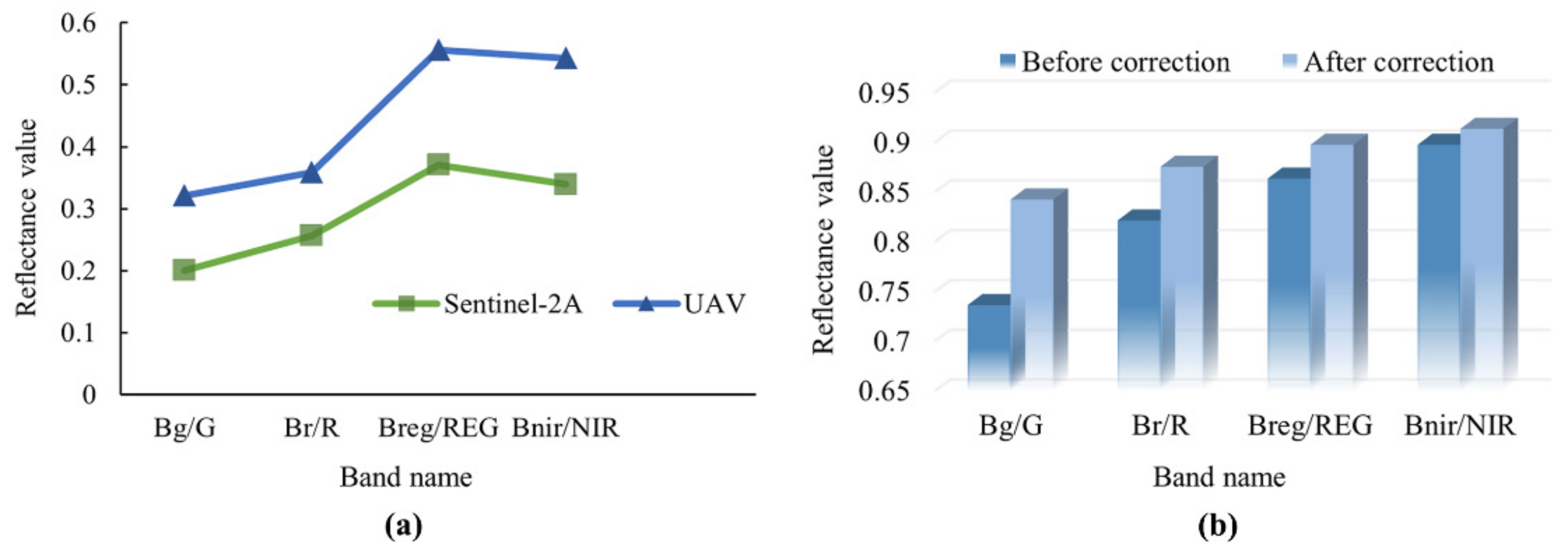
3.2. Reflectance Correction of Sentinel-2A Multispectral Imagery

It is clear from the chart that the reflectivity of each band of the UAV multispectral imagery was slightly higher than that of the Sentinel-2A satellite imagery (Figure 7). The reflectivities of the two bands of Bnir/NIR and Breg/REG were generally higher. However, the reflectance values of the Bg/G, Bnir/NIR, Breg/REG, and Br/R bands showed the same trend. In addition, the order of the correlation coefficients of the reflectance of the two bands before the correction was Bnir/NIR (0.897) > Breg/REG (0.863) > Br/R (0.821) > Bg/G (0.736), with all greater than 0.7 (p > 0.01). From the above results, it can be observed that there is a strong correlation between the various bands of the UAV multispectral imagery and Sentinel-2A satellite imagery, and it is highly feasible for them to perform reflectance correction and estimation.
Therefore, the ratio mean method was used to correct the reflectivity of the two. The reflectivity correction coefficients of each band of Sentinel-2A satellite imagery, calculated based on the reflectivity of the UAV multispectral imagery, are shown in Table 8. The results show that the waveband reflectance correction coefficients of the imagery were all between 0.60 and 0.75. After correction processing, the correlation coefficients between the UAV multispectral imagery and their corresponding band reflectances were greater than 0.8. It has been proven that the combination of satellite–aircraft multi-source remote sensing data for reflectivity correction is beneficial for guaranteeing the accuracy of subsequent soil salinity estimation, and it has the feasibility of estimation.

3.3. Verification and Estimation of the Best Prediction Model of Soil Salinity

3.3.1. Verification of the Best Prediction Model

The optimal prediction model for soil salinity based on UAV multispectral imagery was applied to Sentinel-2A satellite imagery before and after reflectance correction. The comparison results of the model and verification accuracy are shown in Table 9. There are two cases: (1) The best prediction model for soil salinity was applied to Sentinel-2A satellite imagery without reflectivity correction. (2) The best prediction model for soil salinity was applied to Sentinel-2A satellite imagery after reflectivity correction.
The results show that the modeling and verification accuracy of model (2) is superior, while the satellite–machine combination is feasible and conducive to large-scale soil salinity estimation in the subsequent study area.

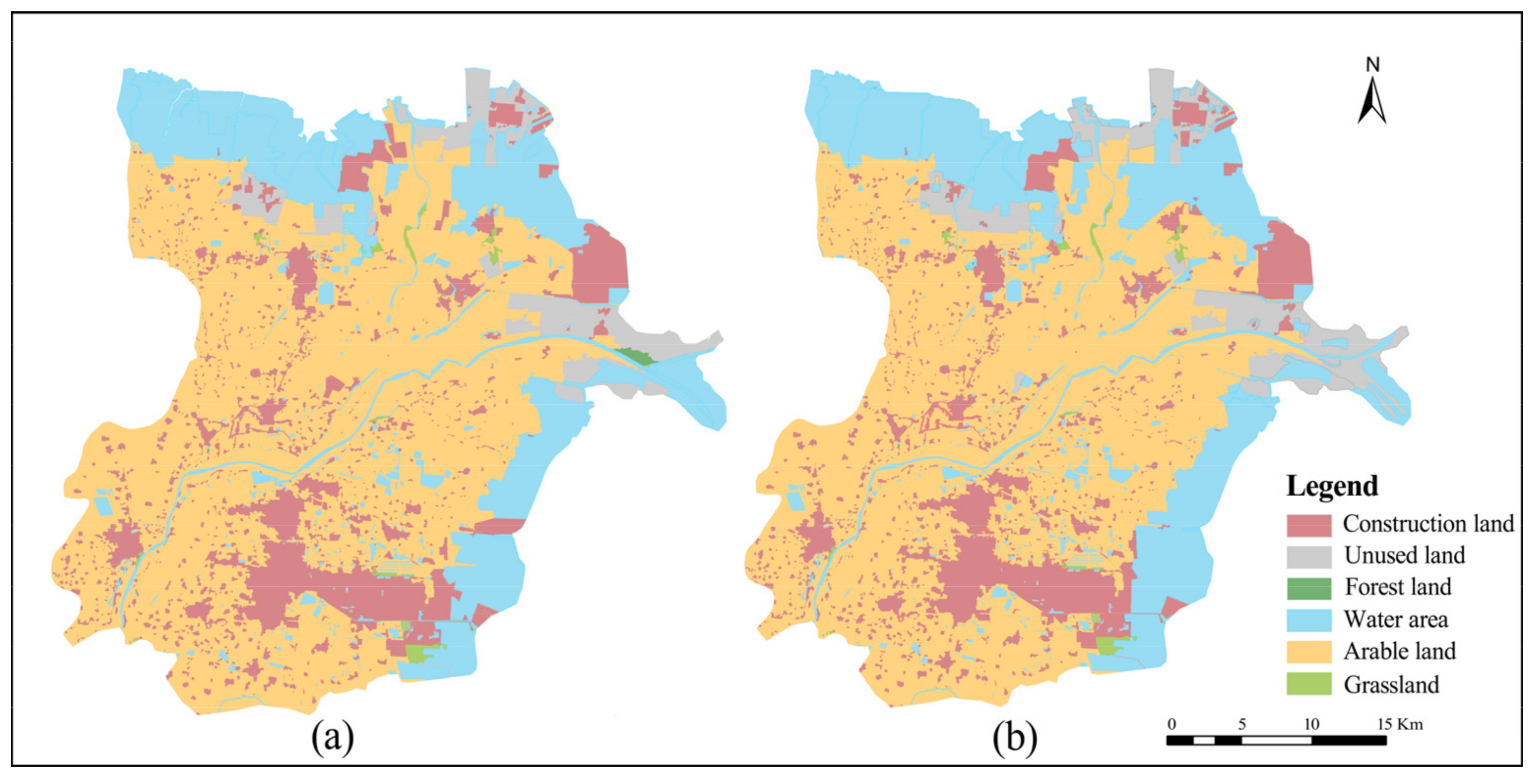
3.3.2. Estimation of Soil Salinity

(1)
Estimation of soil salinity in test area based on UAV multispectral imagery
The estimation results for the soil salinity content in the experimental area are shown in Figure 8. The estimation results were classified according to the classification standard of coastal saline soil with chloride-dominated soil soluble salts in a semi-humid area of China, with the area proportion calculated [3,21,53,59].
The results showed that the estimation value of soil salinity in the experimental area ranged from 0.194 to 21.04 g·kg−1, with an average value of 7.76 g·kg−1 and a standard deviation of 5.81 g·kg−1, which is consistent with the descriptive statistical results of the study area. In addition, the estimation results showed that the percentage of soil salinity content was either extremely high (SC > 20 g·kg−1) or extremely low pixel value (SC < −2 g·kg−1) and was controlled within 10%. Overall, the five grades of saline soil were distributed in the test area. The area of severe-saline soil and solonchak was the largest, reaching 30.67% and 39.19%, respectively, while the proportion of non-saline soil was the lowest (1.56%). Additionally, the proportion of saline soil in the test area for mild-saline soil and moderate-saline soil was 9.35% and 19.23%, respectively. Specifically, the soil salinity content of test area 1 was relatively high, while the heavily salinized soil and saline soil were the most widely distributed, showing a high distribution in the east, low in the west, high in the north, and low in the south. The overall soil salinity in test area 2 was lower than that of test area 1. The distribution of different grades of saline soil was relatively scattered, with the salt content in the middle relatively high, mainly in severely saline and saline soils. The soil salinity estimation in the experimental area showed good results, consistent with the actual situation obtained during the field investigation.
(2)
Retrieval of soil salinity in the study area based on Sentinel-2A satellite imagery
Based on the Sentinel-2A satellite imagery after reflectance correction and the best estimation model, a spatial distribution map of the soil salinity content in the study area in 2019 was obtained (Figure 9a). The ENVI pixel statistics showed that the percentages of extremely low (SC < −2 g·kg−1) or extremely high (SC > 20 g·kg−1) pixel values in the soil salinity estimation results in 2019 were all within 15%, indicating that these results were basically reliable.
From a spatial point of view, the overall distribution trend of soil salinity in the study area in 2019 gradually decreased from northeast to southwest, with moderately and severely salinized soils and saline soils dominating, and very little distribution of non-salinized soils. The overall salinization phenomenon was comparatively serious. The overall soil salinity in the study area is relatively high, and the problem of salinization is correspondingly serious, indicating that the area of moderately saline soil accounted for the highest (43.33%) and the area of non-saline soil accounted for the lowest (2.82%). The proportion of saline soil in the test area for mild-saline soil, severe-saline soil, and solonchak was 15.17%, 28.48%, and 10.2%, respectively. These results are similar to the actual situation in the study area and that described in previous studies [6,60,61].

3.4. Soil Salinity Dynamics in the YRD

3.4.1. Temporal Variation of Soil Salinity

The best salinity prediction model was applied to the reflectance-corrected Sentinel-2A multispectral imagery of March 2016 in the study area (Figure 9b). Based on the pixel statistics in the ENVI software, it is clear that the percentages of extremely low values (SC < −2 g·kg−1) or extremely high values (SC > 20 g·kg−1) that appear in the estimation results of soil salinity in the study area were within 15%. Although the predicted values of severe-saline soils may be low, the results are basically within the normal range. Some of the high salinity areas (mainly in the eastern coastal areas) still showed a trend of increasing salinity, while some of the low salinity areas (mainly located along the Yellow River with richer irrigation water and near the ancient Yellow River ancient road) showed a trend of decreasing salinity content. Overall, the soil salinity in the study area was severe, but the soil salinity coefficients of variation were 0.51 and 0.78 in the study area in 2016 and 2019, respectively, which were less than 1.0. To sum up, the interannual variation of soil salinity was not strong (0.27) and was classified as a medium degree of variation.
Table 10 shows that the degree of change of saline soil area in the study area during 2016–2019 was from mild-saline soil > moderate-saline soil > severe-saline soil > non-saline soil > solonchak, where the stability of mild and moderate saline soil was the weakest and easily transformed with other types of saline soil. Meanwhile, the overall trend of soil salinity in the study area was slightly increasing. Spatially, compared with 2016, the distribution of both severe-saline soil and solonchak within different counties of the study area increased in 2019. Although soil salinity began to accumulate in the areas on both sides of the inlet, the overall change in salinity coverage area was minuscule. The results of different levels of DRi showed that the non-saline soil, mild-saline soil, and solonchak in the study area changed at the fastest rate during 2016–2019, while both moderately and severely saline soil showed a lower degree of expansion (DRi = 0.278 and 0.352, respectively).

3.4.2. The Ground Feature Stability of Saline Soil

As can be seen from Figure 10, the area of arable land in the study area was most widely distributed in both 2016 and 2019, followed by water area mainly in the eastern coastal area and the northern region. Due to the influence of topography, construction land was mainly distributed in the southeastern and northeastern regions of the YRD area. Unused land was mainly distributed near the water area and arable land, and mostly concentrated in the north and east of the study area. The distribution of forest land and grassland occupied a relatively tiny area.
In addition, the dynamics degree in land use motility in the study area from 2016 to 2019 had varying degrees of variation (Table 11), with only 0.152 and 0.058 in construction land and arable land, respectively. While it has a faster rate of change in forest land and grassland, there is an increasing trend of unused land in the eastern coastal region (K of 0.847).
Statistical analysis of the area of different classes of saline soils was based on the feature types in the study area (Table 12). From 2016 to 2019, the area shares of non-saline soil and mild-saline soil distributed on the four feature types showed a negative trend, while the area share of moderately saline soil, severely saline soil, and solonchak showed a positive trend, which was more serious and consistent with the trend in Table 10. In addition, the average area share of different classes of saline soils distributed on four land use types changed from unused land > grassland > forest land > arable land in descending order, where the area share of severe-saline soil distributed on unused land changed the most (89.142%) and the area share of non-saline soil distributed on grassland changed the least (−12.149%). Although the degree of change in the area share of saline soil in arable land was the lowest among the four types of land (19.421%), the change in the area share of moderate-saline soil was the highest (66.914%). The above results indicate that unreasonable tillage has the risk of increasing soil salinization.

4. Discussion

4.1. Estimation Method and Accuracy Verification of Soil Salinity

Using multi-source data for soil salinity estimation, especially after data from different sensors are added to estimation research and analysis, improving spectral consistency is the key to the efficient and accurate monitoring of soil salinity. In this study, the reflectivity of the Sentinel-2A satellite imagery band was slightly lower than that of the UAV multispectral imagery, but the changes in reflectivity in each band of the two methods were consistent. After the reflectivity correction of the two, they show an ideal correlation. They can realize large-scale soil salinity estimation in the study area based on the combination of satellite–computer data and, at the same time, ensure the consistency of soil salinity estimation results with the actual situation.
Soil salinity prediction models exhibit a certain degree of uncertainty. Firstly, the input variables of the soil salinity prediction model were the spectral parameters calculated by the UAV near-ground imagery after the conversion of different bands and various vegetation and salinity indices. The modeling prediction variables are the soil samples measured after drying, grinding, and sieving. The salinity content obtained by the conversion of the conductivity of the formula is different from the actual situation, so the model established based on this has a certain modeling error [36,42,62]. Secondly, although the imagery imaging time should be as close to the sample collection time as possible, there is still a time difference of 5–20 days, which will increase the error of soil salinity monitoring to a certain extent. The percentages of extremely low or extremely high pixel values in the estimation of the experimental area and the study area in different periods were less than 10% and 15%, respectively. The results showed that the estimation was normal, although the high degree of salinized soil content may have been underestimated. This will affect the absolute value of soil salinity but has little effect on the analysis of the multi-year temporal and spatial variation trends and spatial distribution patterns of soil salinity in the entire study area.
Combined with the analysis of the elevation map of the study area (Figure 1), the central and eastern parts of the YRD region are prone to soil salinization due to their low elevation, flat terrain, and slight inclination toward the coast. The overall elevation in the southwest is higher, some mountainous areas are distributed, and the phenomenon of salt accumulation is weaker than that in the central and eastern regions. One of the key characteristics of soil salinization is that it is stable and stubborn, while the activity of nutrients is low and it is generally not easy to change without obvious external forces [35,53]. Combined with the estimation results, the sampling period in this study was in the middle of the ecological water replenishment period of the Yellow River basin in March. Although moderately salinized, severely salinized, and saline soils were distributed in the southwestern part of the study area, the estuary and banks of the Yellow River were all distributed. The soil salinity in this region was not high [53]. Therefore, targeted flow management of the Yellow River is of great significance in improving soil salinization in the YRD.

4.2. Soil Salinity Dynamics and Its Relationship with Land Use

Due to the differences in regional land use, physical stability, and human activities, the salt content of the surface soil in the YRD showed interannual fluctuations of different degrees. The central–eastern part of the YRD region is prone to soil salinization due to its low elevation and flat topography, which makes it easy for salinity to accumulate on the surface and makes the ecological environment extremely fragile. In the southwestern part, the overall elevation is higher and there is some mountainous distribution, so the salinity aggregation phenomenon is relatively weak (Figure 1). The salinity estimation results showed that saline soils in the YRD are widely distributed, with salinization still expanding overall. However, the reason that the salinization phenomenon did not significantly intensify in 2019 compared with 2016 is that one of the key characteristics of soil salinization is its stability and stubbornness, with low activity of nutrients. Consequently, it is generally not easy to change under conditions without obvious external forces. In addition, the sampling period of this research was in March, which was in the middle stage of the ecological recharge period of the Yellow River basin. Although there was an increasing trend of soil salt content in the southwestern part of the study area, the soil salt content in the estuary and the riparian area of the Yellow River was not high [53]. Therefore, targeted flow management of the Yellow River is crucial for improving soil salinity in the YRD.
The year-to-year variation of the area share of different classes of saline soils distributed in different land types was significant. However, the field survey proved that the construction of the Yellow River Estuary Nature Reserve provided a better guarantee to stifle soil salinization and maintain biodiversity in the YRD region. In addition, as the land use type with the largest area share in the study area, the area share of moderate-saline soil on cultivated land varied as high as 53.334% from 2016 to 2019. The results overall indicate that irrational tillage has the risk of increasing soil salinization. Therefore, the protection and ecological development of the soil and land in the YRD cannot be delayed.
The YRD region is affected by its own land formation time conditions as well as unreasonable land use and development, resulting in the overall poor soil quality in the study area. Therefore, the land suitability development model should be further strengthened and land use should be reasonably planned. In addition, in recent years, the arable land in the YRD has increased significantly. In pursuit of high output, there is much unreasonable farming and excessive application of chemical fertilizers, which have led to different degrees of increase in soil salinity in the existing arable land. Therefore, in order to prevent the aggravation of salinization, it is necessary to insist on both saline land management and optimization of agricultural production methods. The measures to balance agricultural development and ecological environmental protection include reasonable tillage and irrigation, promotion of soil formula fertilization, organic and chemical fertilizer application, and adjustment of planting structure.

5. Conclusions

In this research, multi-source field measurement data of soil salinity, UAV, and Sentinel-2A multispectral imagery were fused to construct estimation models of soil salinity at different scales in the YRD. The correction process of reflectance between different images was conducted using the ratio mean method, and finally the inversion of soil salinity in the test and study areas was achieved. In addition, the characteristics of spatial and temporal dynamic variability of soil salinity and its relationship with land use in the Yellow River Delta region from 2016 to 2019 were explored and analyzed. Finally, both high-precision inversion and dynamic analysis of soil salinity based on multi-source data were realized. The main conclusions are as follows:
(1)
Among the different spectral indices, some single bands, vegetation indices, and salinity indices, which are more sensitive to soil salinity, were screened. The BPNN modeling method (R2 = 0.769, RMSE = 2.342 for the modelling set; R2 = 0.774, RMSE = 2.475, RPD = 1.799 for the validation set) and the comprehensive estimation model had the best predicting effect of soil salinity in the Yellow River Delta region.
(2)
Sentinel-2A satellite imagery and UAV imagery reflectance correction can solve the problem of band reflectance and correlation in multi-source data fusion.
(3)
The anomalous values of the estimation results were within 10% and 15% in the test area and study area during 2016–2019, which was consistent with the actual situation. Meanwhile, it shows that the best prediction model of this study can, to a certain extent, realize large-scale estimation of satellite imagery of different periods after reflectance correction.
Because the resolutions of the UAV and Sentinel-2A imagery are to a certain extent different, the spectral fusion problem caused by this difference can be further studied. In addition, there was a strong correlation between soil moisture and salinity in the YRD region. The advantages of satellite–aircraft multi-source remote sensing data can further achieve high-precision extraction and estimation of regional water and salt information while ensuring the spectral characteristics of the two, which is conducive to providing new ideas for the comprehensive improvement of saline–alkali land and optimization of the ecological environment in the YRD region.

Author Contributions

Conceptualization, Z.Z.; Methodology, Z.Z., B.N. and X.K.; Software, Z.Z. and X.K.; Validation, Z.Z.; Visualization, Z.Z.; Formal analysis, Z.Z.; Investigation, Z.Z. and B.N.; Data curation, Z.Z.; Writing—original draft preparation, Z.Z.; Writing—review and editing, Z.Z., B.N., X.L., X.K. and Z.H.; Supervision, B.N., X.L. and Z.H.; Funding acquisition, B.N. and Z.H. All authors have read and agreed to the published version of the manuscript.

Funding

This work was supported by the National Natural Science Foundation of China (NSFC, grant number 41807004), the Postdoctoral Science Foundation of China (PSFC, grant number 2017M622237), and the National Natural Science Foundation of China (NSFC, grant number 41771542).

Data Availability Statement

The datasets used and/or analyzed during the current study are available from the corresponding author on reasonable request.

Acknowledgments

Thank you to the Institute of Land Reclamation and Ecological Reconstruction and X.L.’s research team for their help in this research, to the ESA for support with the Sentinel-2A MSI imagery.

Conflicts of Interest

The authors declare that they have no known competing financial interests or personal relationships that could have appeared to influence the work reported in this paper.

References

  1. Fan, X.; Pedroli, B.; Liu, G.; Liu, Q.; Liu, H.; Shu, L. Soil salinity development in the yellow river delta in relation to groundwater dynamics. Land Degrad. Dev. 2012, 23, 175–189. [Google Scholar] [CrossRef]
  2. Lu, Q.S.; Kang, L.Y.; Shao, H.B.; Zhao, Z.P.; Chen, Q.; Bi, X.L.; Shi, P. Investigating marsh sediment dynamics and its driving factors in Yellow River delta for wetland restoration. Ecol. Eng. 2016, 90, 307–313. [Google Scholar] [CrossRef]
  3. Chen, H.Y.; Zhao, G.X.; Li, Y.H.; Wang, D.Y.; Ma, Y. Monitoring the seasonal dynamics of soil salinization in the Yellow River delta of China using Landsat data. Nat. Hazards Earth Syst. Sci. 2019, 19, 1499–1508. [Google Scholar] [CrossRef] [Green Version]
  4. Ma, Y.; Chen, H.Y.; Zhao, G.X.; Wang, Z.R.; Wang, D.Y. Spectral Index Fusion for Salinized Soil Salinity Inversion Using Sentinel-2A and UAV Images in a Coastal Area. IEEE Access 2020, 8, 159595–159608. [Google Scholar] [CrossRef]
  5. Guo, B.; Zang, W.Q.; Luo, W.; Wen, Y.; Yang, F.; Han, B.M.; Fan, Y.W.; Chen, X.; Qi, Z.; Wang, Z.; et al. Detection model of soil salinization information in the Yellow River Delta based on feature space models with typical surface parameters derived from Landsat8 OLI image. Geomat. Nat. Hazards Risk 2020, 11, 288–300. [Google Scholar] [CrossRef]
  6. Sun, H.Z.; Xu, L.R.; Wang, J.; Fu, X. Remote Sensing Monitoring of Spatial-Temporal Variation of Soil Salinization before and after Irrigation in the Yellow River Delta. J. Coast. Res. 2020, 105, 56–60. [Google Scholar] [CrossRef]
  7. Wang, J.Z.; Ding, J.L.; Yu, D.L.; Ma, X.K.; Zhang, Z.P.; Ge, X.Y.; Teng, D.X.; Li, X.H.; Liang, J.; Lizag, A.; et al. Capability of Sentinel-2 MSI data for monitoring and mapping of soil salinity in dry and wet seasons in the Ebinur Lake region, Xinjiang, China. Geoderma 2019, 353, 172–187. [Google Scholar] [CrossRef]
  8. Xu, C.; Zeng, W.Z.; Huang, J.S.; Wu, J.W.; van Leeuwen, W.J.D. Prediction of Soil Moisture Content and Soil Salt Concentration from Hyperspectral Laboratory and Field Data. Remote Sens. 2016, 8, 42. [Google Scholar] [CrossRef] [Green Version]
  9. Meng, B.P.; Ge, J.; Liang, T.G.; Yang, S.X.; Gao, J.L.; Feng, Q.S.; Cui, X.; Huang, X.D.; Xie, H.J. Evaluation of Remote Sensing Inversion Error for the Above-Ground Biomass of Alpine Meadow Grassland Based on Multi-Source Satellite Data. Remote Sens. 2017, 9, 372. [Google Scholar] [CrossRef] [Green Version]
  10. Hu, X.; Niu, B.B.; Li, X.J.; Min, X.Y. Unmanned aerial vehicle (UAV) remote sensing estimation of wheat chlorophyll in subsidence area of coal mine with high phreatic level. Earth Sci. Inf. 2021, 14, 2171–2181. [Google Scholar] [CrossRef]
  11. Wang, N.; Xue, J.; Peng, J.; Biswas, A.; He, Y.; Shi, Z. Integrating Remote Sensing and Landscape Characteristics to Estimate Soil Salinity Using Machine Learning Methods: A Case Study from Southern Xinjiang, China. Remote Sens. 2020, 12, 4118. [Google Scholar] [CrossRef]
  12. Wei, G.F.; Li, Y.; Zhang, Z.T.; Chen, Y.W.; Chen, J.Y.; Yao, Z.H.; Lao, C.C.; Chen, H.F. Estimation of soil salt content by combining UAV-borne multispectral sensor and machine learning algorithms. Peerj 2020, 8, e9087. [Google Scholar] [CrossRef]
  13. Zhao, D.X.; Wang, J.; Zhao, X.Y.; Triantafilis, J. Clay content mapping and uncertainty estimation using weighted model averaging. Catena 2022, 209, 14. [Google Scholar] [CrossRef]
  14. Zhao, W.J.; Zhou, C.; Zhou, C.Q.; Ma, H.; Wang, Z.J. Soil Salinity Inversion Model of Oasis in Arid Area Based on UAV Multispectral Remote Sensing. Remote Sens. 2022, 14, 1804. [Google Scholar] [CrossRef]
  15. Huang, J.; Koganti, T.; Santos, F.A.M.; Triantafilis, J. Mapping soil salinity and a fresh-water intrusion in three-dimensions using a quasi-3d joint-inversion of DUALEM-421S and EM34 data. Sci. Total Environ. 2017, 577, 395–404. [Google Scholar] [CrossRef]
  16. Zhao, D.X.; Li, N.; Zare, E.; Wang, J.; Triantafilis, J. Mapping cation exchange capacity using a quasi-3d joint inversion of EM38 and EM31 data. Soil Tillage Res. 2020, 200, 12. [Google Scholar] [CrossRef]
  17. El Hajj, M.; Baghdadi, N.; Zribi, M.; Bazzi, H. Synergic Use of Sentinel-1 and Sentinel-2 Images for Operational Soil Moisture Mapping at High Spatial Resolution over Agricultural Areas. Remote Sens. 2017, 9, 1292. [Google Scholar] [CrossRef] [Green Version]
  18. Sui, J.; Qin, Q.M.; Ren, H.Z.; Sun, Y.H.; Zhang, T.Y.; Wang, J.D.; Gong, S.H. Winter Wheat Production Estimation Based on Environmental Stress Factors from Satellite Observations. Remote Sens. 2018, 10, 962. [Google Scholar] [CrossRef] [Green Version]
  19. An, D.Y.; Zhao, G.X.; Chang, C.Y.; Wang, Z.R.; Li, P.; Zhang, T.R.; Jia, J.C. Hyperspectral field estimation and remote-sensing inversion of salt content in coastal saline soils of the Yellow River Delta. Int. J. Remote Sens. 2016, 37, 455–470. [Google Scholar] [CrossRef]
  20. Wang, J.Q.; Peng, J.; Li, H.Y.; Yin, C.Y.; Liu, W.Y.; Wang, T.W.; Zhang, H.P. Soil Salinity Mapping Using Machine Learning Algorithms with the Sentinel-2 MSI in Arid Areas, China. Remote Sens. 2021, 13, 305. [Google Scholar] [CrossRef]
  21. Wang, D.Y.; Chen, H.Y.; Wang, Z.R.; Ma, Y. Inversion of soil salinity according to different salinization grades using multi-source remote sensing. Geocarto Int. 2022, 37, 1274–1293. [Google Scholar] [CrossRef]
  22. Yang, N.; Yang, S.; Cui, W.X.; Zhang, Z.T.; Zhang, J.R.; Chen, J.Y.; Ma, Y.; Lao, C.C.; Song, Z.S.; Chen, Y.W. Effect of spring irrigation on soil salinity monitoring with UAV-borne multispectral sensor. Int. J. Remote Sens. 2021, 42, 8952–8978. [Google Scholar] [CrossRef]
  23. Mandal, A.K. The need for the spectral characterization of dominant salts and recommended methods of soil sampling and analysis for the proper spectral evaluation of salt affected soils using hyper -spectral remote sensing. Remote Sens. Lett. 2022, 13, 588–598. [Google Scholar] [CrossRef]
  24. Shrestha, R.P. Relating soil electrical conductivity to remote sensing and other soil properties for assessing soil salinity in northeast Thailand. Land Degrad Dev. 2006, 17, 677–689. [Google Scholar] [CrossRef]
  25. Allbed, A.; Kumar, L.; Aldakheel, Y.Y. Assessing soil salinity using soil salinity and vegetation indices derived from IKONOS high-spatial resolution imageries: Applications in a date palm dominated region. Geoderma 2014, 230, 1–8. [Google Scholar] [CrossRef]
  26. Zhou, X.H.; Zhang, F.; Zhang, H.W.; Zhang, X.L.; Yuan, J. A Study of Soil Salinity Inversion Based on Multispectral Remote Sensing Index in Ebinur Lake Wetland Nature Reserve. Spectrosc. Spect. Anal. 2019, 39, 1229–1235. [Google Scholar] [CrossRef]
  27. Masoud, A.A. Predicting salt abundance in slightly saline soils from Landsat ETM plus imagery using Spectral Mixture Analysis and soil spectrometry. Geoderma 2014, 217, 45–56. [Google Scholar] [CrossRef]
  28. Yu, H.; Liu, M.Y.; Du, B.J.; Wang, Z.M.; Hu, L.J.; Zhang, B. Mapping Soil Salinity/Sodicity by using Landsat OLI Imagery and PLSR Algorithm over Semiarid West Jilin Province, China. Sensors 2018, 18, 1048. [Google Scholar] [CrossRef] [Green Version]
  29. Peng, J.; Biswas, A.; Jiang, Q.S.; Zhao, R.Y.; Hu, J.; Hu, B.F.; Shi, Z. Estimating soil salinity from remote sensing and terrain data in southern Xinjiang Province, China. Geoderma 2019, 337, 1309–1319. [Google Scholar] [CrossRef]
  30. Wang, Y.; Xie, M.D.; Hu, B.F.; Jiang, Q.S.; Shi, Z.; He, Y.F.; Peng, J. Desert Soil Salinity Inversion Models Based on Field In Situ Spectroscopy in Southern Xinjiang, China. Remote Sens. 2022, 14, 4962. [Google Scholar] [CrossRef]
  31. Guo, B.; Han, B.M.; Yang, F.; Fan, Y.W.; Jiang, L.; Chen, S.T.; Yang, W.N.; Gong, R.; Liang, T. Salinization information extraction model based on VI-SI feature space combinations in the Yellow River Delta based on Landsat 8 OLI image. Geomat. Nat. Hazards Risk 2019, 10, 1863–1878. [Google Scholar] [CrossRef] [Green Version]
  32. Taghadosi, M.M.; Hasanlou, M.; Eftekhari, K. Retrieval of soil salinity from Sentinel-2 multispectral imagery. Eur. J. Remote Sens. 2019, 52, 138–154. [Google Scholar] [CrossRef] [Green Version]
  33. Wu, D.; Jia, K.L.; Zhang, X.D.; Zhang, J.H.; Abd El-Hamid, H.T. Remote Sensing Inversion for Simulation of Soil Salinization Based on Hyperspectral Data and Ground Analysis in Yinchuan, China. Nat. Resour. Res. 2021, 30, 4641–4656. [Google Scholar] [CrossRef]
  34. Hassani, A.; Azapagic, A.; Shokri, N. Predicting long-term dynamics of soil salinity and sodicity on a global scale. Paroc. Natl. Acad. Sci. USA 2020, 117, 33017–33027. [Google Scholar] [CrossRef]
  35. Wang, Z.R.; Zhao, G.X.; Gao, M.X.; Chang, C.Y. Spatial variability of soil salinity in coastal saline soil at different scales in the Yellow River Delta, China. Environ. Monit. Assess 2017, 189, 80. [Google Scholar] [CrossRef]
  36. Zhang, T.R.; Zhao, G.X.; Gao, M.X.; Wang, Z.R.; Jia, J.C.; Li, P.; An, D.Y. Soil Salinity Estimation Based on Near-Ground Multispectral Imagery in Typical Area of the Yellow River Delta. Spectrosc. Spect. Anal. 2016, 36, 248–253. [Google Scholar] [CrossRef]
  37. Bui, E.N. Soil salinity: A neglected factor in plant ecology and biogeography. J. Arid Environ. 2013, 92, 14–25. [Google Scholar] [CrossRef]
  38. Mau, Y.; Porporato, A. A dynamical system approach to soil salinity and sodicity. Adv. Water Resour. 2015, 83, 68–76. [Google Scholar] [CrossRef] [Green Version]
  39. Yao, R.J.; Yang, J.S.; Wu, D.H.; Xie, W.P.; Gao, P.; Wang, X.P. Geostatistical monitoring of soil salinity for precision management using proximally sensed electromagnetic induction (EMI) method. Environ. Earth Sci. 2016, 75, 1362. [Google Scholar] [CrossRef]
  40. Zhang, Z.X.; Song, Y.T.; Zhang, H.Z.; Li, X.J.; Niu, B.B. Effect of different improvement modes on physical and chemical characters of the coastal saline soil. Chin. J. Appl. Ecol. 2021, 32, 1393–1405. [Google Scholar] [CrossRef]
  41. Zhen, Y.; Wu, Z.P.; Yin, Z.H.; Yang, X.Q.; Zhao, X.H. Study on spatio-temporal change of land use in Zoige County, Sichuan Province. Ecol. Sci. 2022, 41, 41–49. [Google Scholar] [CrossRef]
  42. Zhang, C.; Lu, D.S.; Chen, X.; Zhang, Y.M.; Maisupova, B.; Tao, Y. The spatiotemporal patterns of vegetation coverage and biomass of the temperate deserts in Central Asia and their relationships with climate controls. Remote Sens. Environ. 2016, 175, 271–281. [Google Scholar] [CrossRef]
  43. Alhammadi, M.S.; Glenn, E.P. Detecting date palm trees health and vegetation greenness change on the eastern coast of the United Arab Emirates using SAVI. Int. J. Remote Sens. 2008, 29, 1745–1765. [Google Scholar] [CrossRef]
  44. Bannari, A.; El-Battay, A.; Bannari, R.; Rhinane, H. Sentinel-MSI VNIR and SWIR Bands Sensitivity Analysis for Soil Salinity Discrimination in an Arid Landscape. Remote Sens. 2018, 10, 855. [Google Scholar] [CrossRef] [Green Version]
  45. Huete, A.; Didan, K.; van Leeuwen, W.; Vermote, E. Global-scale analysis of vegetation indices for moderate resolution monitoring of terrestrial vegetation. In Proceedings of the Remote Sensing for Earth Science, Ocean, and Sea Ice Applications, Florence, Italy, 20–24 September 1999; Volume 3868, pp. 141–151. [Google Scholar] [CrossRef]
  46. Douaoui, A.E.K.; Nicolas, H.; Walter, C. Detecting salinity hazards within a semiarid context by means of combining soil and remote-sensing data. Geoderma 2006, 134, 217–230. [Google Scholar] [CrossRef]
  47. Abbas, A.; Khan, S.; Hussain, N.; Hanjra, M.A.; Akbar, S. Characterizing soil salinity in irrigated agriculture using a remote sensing approach. Phys. Chem. Earth 2013, 55–57, 43–52. [Google Scholar] [CrossRef]
  48. Khan, N.M.; Rastoskuev, V.V.; Sato, Y.; Shiozawa, S. Assessment of hydrosaline land degradation by using a simple approach of remote sensing indicators. Agr. Water Manag. 2005, 77, 96–109. [Google Scholar] [CrossRef]
  49. Wu, W.C. The Generalized Difference Vegetation Index (GDVI) for Dryland Characterization. Remote Sens. 2014, 6, 1211–1233. [Google Scholar] [CrossRef] [Green Version]
  50. Zhang, H.Y.; Fan, J.W.; Shao, Q.Q. Land use/land cover change in the grassland restoration program areas in China, 2000-2010. Prog. Geo. 2015, 34, 840–853. [Google Scholar] [CrossRef]
  51. Crawford, S.B.; Kosinski, A.S.; Lin, H.M.; Williamson, J.M.; Barnhart, H.X. Computer programs for the concordance correlation coefficient. Comput. Meth. Programs Biomed. 2007, 88, 62–74. [Google Scholar] [CrossRef]
  52. Lin, L.I. A concordance correlation coefficient to evaluate reproducibility. Biometrics 1989, 45, 255–268. [Google Scholar] [CrossRef]
  53. Zhang, S.M.; Zhao, G.X. A Harmonious Satellite-Unmanned Aerial Vehicle-Ground Measurement Inversion Method for Monitoring Salinity in Coastal Saline Soil. Remote Sens. 2019, 11, 1700. [Google Scholar] [CrossRef] [Green Version]
  54. Bian, L.L.; Wang, J.L.; Liu, J.; Han, B.M. Spatiotemporal Changes of Soil Salinization in the Yellow River Delta of China from 2015 to 2019. Sustainability 2021, 13, 822. [Google Scholar] [CrossRef]
  55. Qi, G.H.; Chang, C.Y.; Yang, W.; Gao, P.; Zhao, G.X. Soil Salinity Inversion in Coastal Corn Planting Areas by the Satellite-UAV-Ground Integration Approach. Remote Sens. 2021, 13, 3100. [Google Scholar] [CrossRef]
  56. Zare, E.; Arshad, M.; Zhao, D.X.; Nachimuthu, G.; Triantafilis, J. Two-dimensional time-lapse imaging of soil wetting and drying cycle using EM38 data across a flood irrigation cotton field. Agr. Water Manag. 2020, 241, 106383. [Google Scholar] [CrossRef]
  57. Liu, J.; Zhang, L.; Dong, T.; Wang, J.L.; Fan, Y.M.; Wu, H.Q.; Geng, Q.L.; Yang, Q.J.; Zhang, Z.B. The Applicability of Remote Sensing Models of Soil Salinization Based on Feature Space. Sustainability 2021, 13, 3711. [Google Scholar] [CrossRef]
  58. Liu, D.D.; Zhang, Y.J.; Liu, J.; Mei, X.D.; Zhao, X.M.; Zhu, J.W.; Wang, M.S.; Wang, Y.L. Study on Inversion of Soil Salinity with Hyperspectral Remote Sensing. In Proceedings of the 2016 International Conference on Environmental Science and Engineering (Ese 2016), Guilin, China, 15–17 April 2016; pp. 526–530. [Google Scholar]
  59. Chen, H.Y.; Ma, Y.; Zhu, A.X.; Wang, Z.R.; Zhao, G.X.; Wei, Y.A. Soil salinity inversion based on differentiated fusion of satellite image and ground spectra. Int. J. Appl. Earth Obs. 2021, 101, 102360. [Google Scholar] [CrossRef]
  60. Meng, L.; Zhou, S.W.; Zhang, H.; Bi, X.L. Estimating soil salinity in different landscapes of the Yellow River Delta through Landsat OLI/TIRS and ETM plus Data. J. Coast Conserv. 2016, 20, 271–279. [Google Scholar] [CrossRef]
  61. Zhang, M.L.; Wang, H.X.; Pang, X.K.; Liu, H.; Wang, Q. Characteristics of soil salinity in the typical area of Yellow River Delta and its control measures. IOP Conf. Ser. Earth Environ. Sci. 2017, 64, 012078. [Google Scholar] [CrossRef]
  62. Niu, B.B.; Zhang, Z.X.; Yu, X.Y.; Li, X.J.; Wang, Z.; Loaiciga, H.A.; Peng, S. Regime shift of the hydroclimate-vegetation system in the Yellow River Delta of China from 1982 through 2015. Environ. Res. Lett. 2020, 15, 024017. [Google Scholar] [CrossRef]
Figure 1. Sketch map of the research area based on elevation and distribution map of sampling points in the test areas.
Land 11 02307 g001
Figure 2. Methodological scheme of this study.
Land 11 02307 g002
Figure 3. Correlation coefficient between soil salinity and spectral indices.
Land 11 02307 g003
Figure 4. Accuracy statistics of (a) band reflectivity estimation model, (b) vegetation index estimation model, (c) soil salinity index estimation model, and (d) comprehensive estimation model in different modeling methods.
Land 11 02307 g004
Figure 5. Statistics of reflectivity and modeling accuracy for different bands and spectral parameters.
Land 11 02307 g005
Figure 6. (a) Scatter plot for accuracy verification based on the best estimation model of soil salinity according to UAV multispectral imagery. (b) Comparison of the prediction results of soil salinity in the validation set.
Land 11 02307 g006
Figure 7. (a) Comparison of reflectivity between UAV multispectral imagery and Sentinel-2A satellite imagery. (b) Correlation between UAV multispectral imagery and reflectivity of Sentinel-2A imagery before and after correction.
Land 11 02307 g007
Figure 8. Estimation map of soil salt content in the test area.
Land 11 02307 g008
Figure 9. (a) Spatial distribution of soil salt content in the study area in 2019. (b) Spatial distribution of soil salt content in the study area in 2016.
Land 11 02307 g009
Figure 10. (a) Map of land use types in the study area in 2016. (b) Map of land use types in the study area in 2019.
Land 11 02307 g010
Table 1. The corresponding relationship of data between Sentinel-2A imagery and UAV imagery.
Band NameUAV Imagery Data
(Equipped with Sequoia Agricultural Multispectral Camera)
Sentinel-2A Imagery Data
BandCenter Wavelength (nm)FWHMBandCenter Wavelength (nm)
BgB1-Green55020B3-Green560
BrB2-Red66020B4-Red665
Breg1---B5-Vegetation Red Edge705
Breg2B3-Red Edge7355B6-Vegetation Red Edge740
BnirB4-Near IR79020B7-Vegetation Red Edge783
Table 2. Spectral indexes and related formulas.
Index TypeSpectral IndexExpressionReferences
Triangle Vegetation Index (TVI)Normalized Vegetation Index (NDVI) N I R     R N I R   +   R [24]
Difference Vegetation Index (DVI) N I R     R [24]
Soil Adjusted Vegetation Index (SAVI) 1   +   L N I R     R N I R   +   R   +   L L = 0.5 [43]
Ratio Vegetation Index (RVI) N I R R [43]
Green Light Normalized Difference Vegetation Index (GNDVI) N I R     G N I R   +   G [44]
Red Edge Normalized Vegetation Index
(NDVI-reg)
N I R     R E G N I R     R E G [44]
Salinity Index (SI)Salinity Index (SI-T) R NIR × 100 [45]
Salinity Index 1 (SI1) G × R [25]
Salinity Index 2 (SI2) G 2 + R 2 + NIR 2 [46]
Salinity Index 3 (SI3) G 2 + R 2   [46]
Salinity Index 7 (SI7) R   ×   NIR G [47]
Normalized Difference Salinity Index (NDSI) ( R     NIR ) ( R   +   NIR ) [48]
Salinization Remote Sensing Index (SRSI) NDVI     1 2 + SI 1 2 [43]
Brightness Index (BI)Brightness Index (BI) R 2 + NIR 2 [48]
Note: NIR, R, REG, and G in the formulas represent the reflectance values of near-infrared band, red band, red edge band, and green band, respectively.
Table 3. Descriptive statistics of soil samples.
Sample TypeMinimum
(g·kg−1)
Maximum
(g·kg−1)
Average
(g·kg−1)
Standard Deviation
(g·kg−1)
All samples0.25420.6407.5815.736
Modeling set0.26720.6407.5725.725
Validation set0.25420.2307.6215.804
Table 4. Correlation coefficient between soil salinity and UAV’s band.
BandGrey Correlation IndexPearson Correlation Index
Bg0.597 **0.561 **
Br0.599 **0.554 **
Breg0.580 *0.579 *
Bnir0.630 **0.547 **
* Significant at 0.05 level. ** Significant at 0.01 level.
Table 5. Spectral parameters of the band reflectance, vegetation index, and salinity estimation model.
Model TypeSerial NumberSpectral ParametersSerial NumberSpectral Parameters
Band reflectance1Bg7 sin Breg
2Br8 log 2 Bnir
3Breg9 Bg 2 + 5 2
4Bnir10 Breg + 1 Breg 1
5 Bg 2 11 ln Br
6 Br + 2 / 2 Br 12 Bnir × 3
Vegetation index1NDVI9 NDVI × 3
2DVI10 log 2 GNDVI
3SAVI11 SAVI + ln 2
4RVI12 ln SAVI
5GNDVI13 log 3 RVI
6NDVI-reg14 Bg 2 + 5 2
7 3 + NDVI 2 15 NDVI reg + 1 NDVI reg 1
8 DVI + 5 2 DVI 16 sin DVI + cos DVI
Salinity index1SI-T10 SI 1 2 + 3 2
2SI11 log 2 SI 3 / 2
3SI112 SI 7 + ln 2
4SI313 ln SI 7
5SI714 log 3 NDSI
6NDSI15 SI 3 2 + 5 2
7 log 2 SI 16 NDSI + 1 × 1 NDSI
8 3 × SI T + 1 10 sin SI 1
Table 6. Diagnostic index of each band in UAV imagery.
BgBrBregBnir
Ri0.597 **0.599 **0.580 *0.630 **
σi0.7910.7610.4700.532
Pi0.4720.4560.2730.335
* Significant at 0.05 level. ** Significant at 0.01 level.
Table 7. Spectral parameters of comprehensive estimation model of soil salinity.
Serial NumberSpectral ParametersSerial NumberSpectral Parameters
1Bg10 Bg 2 + 5 2
2Br11 Br + 2 / 2 Br
3Bnir12 Bnir × 3 × Bnir + 1
4NDVI13 3 × NDVI
5DVI14 DVI + 5 2 DVI
6GNDVI15 log 2 GNDVI
7SI-T16 3 × SI T + 1
8SI117 sin SI 1
9NDSI18 NDSI + 1 × 1 NDSI
Table 8. Sentinel-2A satellite imagery reflectance correction coefficient for each band.
Band NameGRREGNIR
Coefficient of reflectance correction0.6140.6310.7260.741
Table 9. Comparison of the accuracy of different models before and after reflectivity correction.
ModelModeling AccuracyVerification Accuracy
R2RMSER2RMSERPD
(1)0.4214.050.3994.361.43
(2)0.6373.520.5943.901.69
Table 10. Statistical table of dynamic changes of different types of saline soil.
Types of Saline SoilArea(km2)Area Change
(km2)
DRi
(%)
20162019
Non-saline soil203.257110.440−92.817−1.370
Mild-saline soil851.014594.104−256.910−0.906
Moderate-saline soil1552.8171696.937144.1200.278
Severe-saline soil998.2681115.365117.0970.352
Solonchak310.955399.46588.5100.854
Table 11. The dynamics degree of land use in the study area from 2016 to 2019 (unit: hectares).
Land UseK (%)Land UseK (%)
Grassland0.188Forest land1.484
Arable land0.058Water area1.148
Construction land0.152Unused land0.847
Table 12. Changes in different grades of saline soil based on land use types in the study area from 2016 to 2019 (unit: %).
Types of Saline SoilArea Change (%)
GrasslandArable LandForest LandUnused Land
Non-saline soil−12.149−15.701−19.630−21.710
Mild-saline soil−38.306−23.968−13.134−50.139
Moderate-saline soil46.43866.91438.02034.104
Severe-saline soil74.24053.33469.08389.142
Solonchak29.77719.42125.66148.603
Publisher’s Note: MDPI stays neutral with regard to jurisdictional claims in published maps and institutional affiliations.

