Article

Comparison of Machine Learning-Based Prediction of Qualitative and Quantitative Digital Soil-Mapping Approaches for Eastern Districts of Tamil Nadu, India

by
Ramalingam Kumaraperumal
1,*,
Sellaperumal Pazhanivelan
2,*,
Vellingiri Geethalakshmi
2,
Moorthi Nivas Raj
1,
Dhanaraju Muthumanickam
1,
Ragunath Kaliaperumal
2,
Vishnu Shankar
3,
Athira Manikandan Nair
4,
Manoj Kumar Yadav
5 and
Thamizh Vendan Tarun Kshatriya
4
1
Department of Remote Sensing and GIS, Tamil Nadu Agricultural University, Coimbatore 641003, India
2
Water Technology Centre, Tamil Nadu Agricultural University, Coimbatore 641003, India
3
Department of Physical Science and Information Technology, Tamil Nadu Agricultural University, Coimbatore 641003, India
4
Department of Soil Science and Agricultural Chemistry, Tamil Nadu Agricultural University, Coimbatore 641003, India
5
Deutsche Gesellschaft für Internationale Zusammenarbeit (GIZ) GmbH, New Delhi 110029, India
*
Authors to whom correspondence should be addressed.
Land 2022, 11(12), 2279; https://doi.org/10.3390/land11122279
Submission received: 21 October 2022 / Revised: 10 December 2022 / Accepted: 10 December 2022 / Published: 13 December 2022

Abstract

:
The soil–environmental relationship identified and standardised over the years has expedited the growth of digital soil-mapping techniques; hence, various machine learning algorithms are involved in predicting soil attributes. Therefore, comparing the different machine learning algorithms is essential to provide insights into the performance of the different algorithms in predicting soil information for Indian landscapes. In this study, we compared a suite of six machine learning algorithms to predict quantitative (Cubist, decision tree, k-NN, multiple linear regression, random forest, support vector regression) and qualitative (C5.0, k-NN, multinomial logistic regression, naïve Bayes, random forest, support vector machine) soil information separately at a regional level. The soil information, including the quantitative (pH, OC, and CEC) and qualitative (order, suborder, and great group) attributes, were extracted from the legacy soil maps using stratified random sampling procedures. A total of 4479 soil observations sampled were non-spatially partitioned and intersected with 39 environmental covariate parameters. The predicted maps depicted the complex soil–environmental relationships for the study area at a 30 m spatial resolution. The comparison was facilitated based on the evaluation metrics derived from the test datasets and visual interpretations of the predicted maps. Permutation feature importance analysis was utilised as the model-agnostic interpretation tool to determine the contribution of the covariate parameters to the model’s calibration. The R2 values for the pH, OC, and CEC ranged from 0.19 to 0.38; 0.04 to 0.13; and 0.14 to 0.40, whereas the RMSE values ranged from 0.75 to 0.86; 0.25 to 0.26; and 8.84 to 10.49, respectively. Irrespective of the algorithms, the overall accuracy percentages for the soil order, suborder, and great group class ranged from 31 to 67; 26 to 65; and 27 to 65, respectively. The tree-based ensemble random forest and rule-based tree models’ (Cubist and C5.0) algorithms efficiently predicted the soil properties spatially. However, the efficiency of the other models can be substantially increased by advocating additional parameterisation measures. The range and scale of the quantitative soil attributes, in addition to the sampling frequency and design, greatly influenced the model’s output. The comprehensive comparison of the algorithms can be utilised to support model selection and mapping at a varied scale. The derived digital soil maps will help farmers and policy makers to adopt precision information for making decisions at the farm level leading to productivity enhancements through the optimal use of nutrients and the sustainability of the agricultural ecosystem, ensuring food security.

1. Introduction

Conventional methods for soil surveys involve delineating soil polygons based on the subjective decisions made by the surveyors and are usually presented in printed reports or chart format. The lack of digital forms of soil information can limit the efficiency of several applications, in addition to the inefficiency of the traditional methods in representing the within-class variability and current variability of the respective soil attributes [1,2]. In the last few decades, there has been an evident shift in soil surveys from soil surveyor-based qualitative soil delineation to data-driven quantitative assessment of the soils [3]. The transformation was accelerated mainly due to the increasing need for soil resource information for selecting suitable crops, the area and yield estimation of crops, determining the predominant soil types, delineating the management zones and drainage classes, adopting appropriate land use plans, and identifying potential carbon sequestration zones, among others [4]. With the technical advancements in remote sensing, geographical information systems, and data analysis, a cumulative collection of mapping procedures has been implemented and evolved to increase the accuracy of the methodology and the generated maps. In addition to the soil spectral information, extensive spatial coverage and temporal consistency from remote sensing data can help with the mapping of inaccessible locations [5].
Digital soil mapping aims to link the soil responses to environmental variables through the implication of inference and numerical models. DSM can be defined as “the creation, and population of spatial soil information systems (SSINFOS) by the use of field and laboratory observational methods, coupled with spatial and non-spatial soil inference models”. Further, the need for a self-updating generic framework for spatial soil inference systems (SSINFERS) has been espoused to derive the data requested by users [6]. The processes included in the digital soil-mapping procedures include (1) Generating soil databases for the particular soil attribute of interest; (2) Deriving and selecting the soil environmental covariates based on the SCORPAN factors that better depict the soil attributes; (3) Model calibration, validation, and parameter tuning; (4) Spatial prediction based on the model calibrated; (5) Interpolation or extrapolation of the prediction function if required; and (6) Accuracy assessment based on the independent datasets.
Conventional soil mapping procedures for characterising soil attributes involve destructive soil sampling, aerial photo interpretation, surveying based on vegetation and topography maps, and associated laboratory analyses. These procedures are highly time consuming and expensive when the mapping is performed at national or regional levels in addition to being based on the surveyor’s conceptual or mental model [7,8]. Some of the machine learning techniques that have been adopted so far based on a literature survey that included comparative studies are multiple linear regression (MLR); regression kriging (RK); random forest (RF); quantile regression forest (QRF); support vector machine (SVM); Bayesian networks; neural networks, e.g., artificial neural networks (ANN) and convolutional neural networks; the generalized additive model (GAM); logistic regression; distance-based learners, e.g., k-nearest neighbour (kNN); decision trees, e.g., Cubist (CB); classification and regression tree (CART); C5.0; principal component regression (PCR); partial least square regression (PLSR); extreme learning machines (ELM); boosted regression trees; and ensemble machine learning (EML) [9,10,11,12,13,14,15,16,17,18,19,20,21,22,23,24,25,26,27,28,29,30].
The model’s predictive ability also depends on the quantity and quality of soil samples, especially when derived from multiple resources. The soil samples can be biased as the surveyor collects the data from areas with better accessibility. Moreover, the associated spatial bias can degrade the statistical relationship between the soil samples and covariates generated, which can impede DSM accuracy. Therefore, attention must be focused on improving the predictive ability of the calibrated DSM model by optimising the sampling procedures, hyperparameter settings, nature of the target and covariate attributes, associated spatial supports, and selected covariate selection procedure [31].
With the advent of many specialized machine learning algorithms, comparison and validation of the algorithms are essential to screen for models that provide unreliable and redundant results when the predictions are further upscaled to the state level. Additionally, the problem inherent with most machine learning algorithms is their lack of detailed interpretability. In such cases, explicit quantification of the covariate information using the global agnostic tools was implemented in several studies including the permutation feature importance analysis. The PFI analysis was considered for its computation efficiency and limited parameterisation [32]. The objectives of this study are (1) to generate digital soil class and attribute maps using a suite of six machine learning algorithms; and (2) to compare and validate the digital soil maps based on the visual interpretation and evaluation metrics derived.

2. Materials and Methods
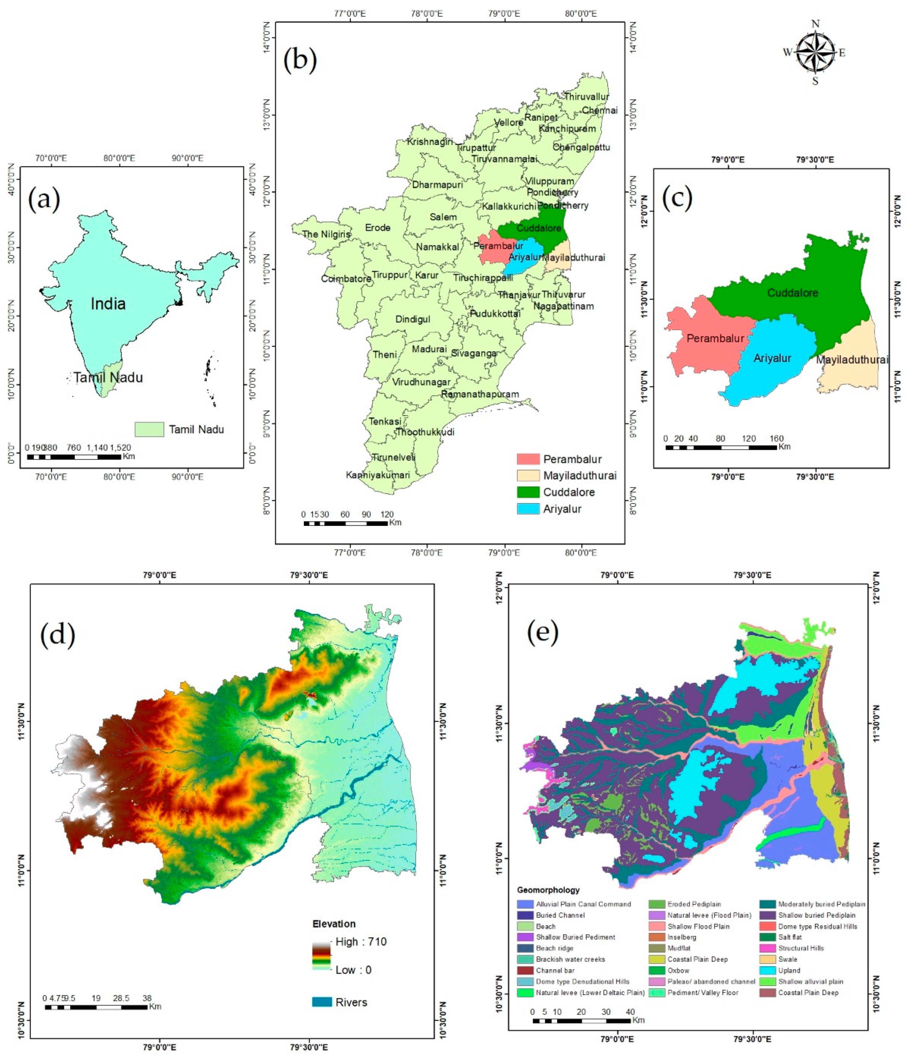
2.1. Study Area

The study area included four districts of Eastern Tamil Nadu, India: Ariyalur, Cuddalore, Mayiladuthurai, and Perambalur. The districts were selected because of their unpredictable climate conditions with greatly varied geomorphological and hydrological characteristics. Given the extremities of the associated factors, the current study also indirectly assessed the potential of the digital soil-mapping procedures to mitigate the shortcomings of mapping regional-level landscapes and delineating the soil attributes. The study area extended geographically from 11°53′22″ to 10°53′15″ N latitude and 78°38′5″ to 79°51′28″ E longitude, collectively covering an area of 8569.21 square km (Figure 1).
The extent of the study area is covered adjacently by the various districts of Tamil Nadu, with coastal regions adjoining the Cuddalore and Mayiladuthurai districts. Ariyalur and Perambalur are considered the inland districts of Tamil Nadu, with nlack and red loam soil as the predominant soil types and a semi-arid climate. In particular, the lands of Ariyalur are characterised by the presence of limestone and ferruginous red loam. At the same time, the Cuddalore and Mayiladuthurai districts have tropical climates with alluvial, sandy loam, and sandy clay loam as the predominant soil textural classes. The study area experiences an annual temperature that varies from 26.81 to 28.01 °C.
Similarly, the annual precipitation of the study area varies from 1351 to 1737 mm from west to east, most of which is contributed by the northeast monsoon downpour. Considering the rain-fed irrigation prevalence of Ariyalur and Perambalur, maize and cotton are the most cultivated crops. In contrast, the Cuddalore and Mayiladuthurai districts are situated in the Cauvery River basin, where the major crops are paddy, pearl millet, maize, and pulses.

2.2. Soil Data

The soil data were extracted from the legacy soil map obtained from the National Resource Information System of NNRMS [33]. A stratified random sampling procedure was used to derive the sampling sites with soil series as a distinctive stratum. A cumulative fraction of each of the 4479 soil observations was sampled, and around 521 sample points corresponding to the habitation, water bodies, and miscellaneous landform elements were included for the soil class delineation. The organic carbon (OC), pH, and cation exchange capacity (CEC) were the continuous soil attributes considered for the digital soil mapping. Similarly, the categorical soil attributes utilised for the delineation were the soil order, suborder, and great group.

2.3. Environmental Covariates

A total of 39 environmental covariates representing the climate, relief, organisms, and parent material were derived from remote sensing and DEM products. Spatially interpolated annual mean temperature and annual rainfall data (global cover) available from WorldClim 2.1 (https://www.worldclim.org/data/worldclim21.html, accessed on 16 March 2021) were downloaded at 30 arc seconds with a temporal range of 1970–2000. Satellite data products with their associated NDVI products in addition to the land use and land cover products were essentially considered the parameters that reflected the organisms’ covariates. The Landsat-8 product (‘LANDSAT/LC08/C01/T1_SR’) depicts the surface reflectance of the study area downloaded from the Google Earth Engine. The data collection was limited to the period from March to May for better delineation of soil properties. A 3-month composite with a median filter was adopted to reduce the effects of cloud cover and shadow effects.
A total of 22 secondary terrain attributes were derived from the Shuttle Radar Topography Mission (SRTM) exclusively through the hydro geomorphometric indexes of the SAGA GIS software. In the case of the parent material covariate, the spectral indices that depict the mineralogy of the study area were derived from the Landsat-8 images. Further, existing soil maps indicating the land use and land cover (organisms) [34], physiography (terrain), and geomorphology (parent material) [35] were obtained from the National Remote Sensing Centre at a 1:50,000 scale and were implemented as the covariate layers. Finally, the derived covariate spatial layers were resampled and reprojected to a 30 m spatial resolution using the ArcGIS 10.6 software. The environmental covariates implemented for the soil attribute delineation are depicted in Table 1.

2.4. Model Development

The model’s training, testing, and spatial depiction of the predicted soil attributes were facilitated through the spatial environment of R. The ithir package and its associated functions for soil-related spatial functions were used in the present study. The visual presentation of the predicted soil attributes was facilitated by ArcGIS software. The packages invoked for the calibration of the machine learning algorithms and their parameterisations are specified in Table 2.

2.4.1. Multiple Linear Regression (MLR)

Multiple linear regression is the most consistently used parametric measure for prediction. MLR determines the linear relationship between the soil attribute and covariates and predicts the outcome of the target attributes by fitting a linear equation with the model parameters (coefficients) [44]. The major constraint of the MLR model is that it does not account for the nonlinear relationship among the variables considered.

2.4.2. Multinomial Logistic Regression (MnLR)

Typically, logistic regression models can describe the binary response variables, where the predictions are defined as the probability of the occurrence (0 and 1) [45]. Multinomial logistic regression predicts the probability of the category membership of the soil attributes based on the covariate predictors [46]. The present study generated logistic regression models for each soil class with default parameter settings [47].

2.4.3. k-Nearest Neighbour (k-NN)

K-nearest neighbour (KNN) is a simple non-parametric classifier based on the known instance to label an unknown instance based on a distance function [48]. The values/classes will be assigned based on the majority classes or average of attributes or on the distance measure implemented, i.e., the Euclidean distance [49]. The k-NN classifier usually requires the data to be normalised for the model calibration, as distance-based learners require the covariates to be in a similar range. The centring and scaling of the datasets were facilitated via the ‘preProcess’ function of the caret package. Further, the k-NN model can be tuned by specifying the number of neighbours (k) within the proximity for the model training. The default parameter setting of the train function with the ‘knn’ method recursively determines the optimal k values by implementing a bootstrap resampling procedure for the model calibration. A k value of 9 was determined from the model calibration for all the soil attributes based on the evaluations of the RMSE (continuous) and overall accuracy (categorical) obtained for other values of k through cross-validation.

2.4.4. Decision Trees (Regression Trees)

The algorithm works by recursively partitioning the datasets and determining the subset that can be further split until the predetermined termination factor is achieved. Decision tree algorithms are generally non-parametric models, and the split associated with the models can be optimised based on passing a control function. The control function can be invoked based on the ‘rpart.control’ parameter. The arguments that are necessarily passed through the ‘rpart.control’ include minsplit (minimum observation in a node for a split to be attempted) and cp (complexity parameter—split that does not decrease the overall lack of fit by the factor of “cp” that is not tried). The ‘rpart’ function was implemented with a ‘minsplit’ of 50 observations. Typically, the default arguments of the ‘rpart’ with a cp of 0.01 with splits based on the “Information” or “gini” index have been determined to be successful at pre-pruning and splitting so that the cross-validation excludes one or two surrogate trees. Still, sometimes it may overprune, especially when the ‘rpart’ is performed on large datasets with a small range [50]. Since splitting the dataset with the default parameter yielded crude and incomparable results, the optimal cost-complexity pruning value (cp) was determined by initially setting the cp value with -Inf. The negative infinity value helps to generate all the maximum possible trees for the datasets. Then, based on the minimum cross-validated error generated, the cp value for pruning was assessed and further fine-tuned regression trees were generated.

2.4.5. Decision Trees (C5.0)

The C5.0 algorithm is a non-parametric and decision tree-based machine learning algorithm that fits the classification trees based on Quinlan’s C5.0 algorithm. The C5.0 algorithm was implemented with the control function defined within the model definition. In general, the implication of trail parameters can help in the implementation of a boosted classification tree process, with the results cumulated at termination [51]. The C5.0 control function was defined in the current study using CF (confidence factor), minCases (minimum number of samples that must be imparted in at least two of the splits), and earlyStopping (a logical that defines whether the internal method for stopping boosting should be used) argument values of 0.95, 20, and FALSE, respectively.

2.4.6. Naïve Bayes (NB) Classifier

A naïve Bayes classifier is a probability-based statistical classifier based on the assumption that the effect of the covariate value on a given class is independent of the values of the other covariates. Referred to as conditional independence, the assumption is made to reduce the associated computational time. Hence, the classifier is termed “Naive” [52]. In short, the classifier assumes that the covariates are completely independent even though some dependency exists between the covariates. The classifier calculates the conditional probabilities of each covariate separately and the a priori chances for each class level.

2.4.7. Support Vector Regression/Machine (SVR/M)

Support vector machine is essentially data classification and a non-parametric technique extended for regression predictions. The SVR/M operates by projecting the data points (support vectors) using hyperplanes and further segregates and groups the datasets, i.e., each segment contains only one kind of data. In cases of SVR/M, the algorithm acknowledges the presence of nonlinearity in the datasets [53]. It calibrates the model by limiting the error associated with the base value (principle of maximal margin). In addition, SVR/M implies kernel functions to predict nonlinear problems by projecting the nonlinear vector to high-dimensional spaces [54]. Based on the object type of the response variable (factor or not), the model instigates the classification or regression of the proposed datasets. With the default parameters included, the number of support vectors is automatically determined for continuous (2788) and categorical (3133) variables, which decides the overall performance of the support vector regression and classification.

2.4.8. Cubist Regression

The Cubist model is the most popular model structure used because of its ability to model the nonlinear relationships associated with the datasets and is an extension of the M5 tree model. Like regression trees (rpart), the parameters are tuned by passing a control function (cubistControl) or control parameter within the model definition [55]. In the present study, values of 100 and 15 were inputted into the rules and extrapolation arguments, respectively.

2.4.9. Random Forest (RF)

Random forest is a boosted decision tree model made by constructing multiple decision trees during training, which are later consolidated to define one single prediction for each observation in the datasets. The average of the individual trees is computed for regression prediction, and for categorical variables, predictions are made on a majority basis [56]. Soil prediction studies consider random forest algorithms for their robust performance and limited need for fine-tuning. The present study implemented fine-tuning by adjusting the ntree (number of trees to be constructed) and mtry (number of covariates selected as candidates at each split) hyperparameters. For spatial prediction of the quantitative soil attributes, an ntree value of 1000 with default mtry values were inputted [57]. For the spatial prediction of the qualitative soil attributes, an ntree value of 500 and mtry of 5 were inputted for pruning the decision trees.

2.5. Model Validation

In order to mitigate the effects of spatial autocorrelation on the validation of the models, spatial partitioning of the datasets was facilitated based on the random holdback procedure. The datasets were partitioned and 70% of the total was sampled for the training dataset and the remaining 30% for validation. We calculated the validation metrics for the quantitative and qualitative soil attributes separately for each predictive model calibrated.

2.5.1. Quantitative Soil Attributes

For the quantitative soil attributes, the coefficient of determination (R2) [a], concordance correlation coefficient (CCC) [b], root mean square error (RMSE) [c], and bias [d] were implemented for determining the quality of the predictions made by each of the machine learning algorithms. The metrics were calculated using the goof function of the ithir package in R.
R 2 = 1 i = 1 n ( p i o i ) 2 i = 1 n ( o i o i ¯ ) 2 [ a ]
C C C = 2 ρ o i p i o i 2 + p i 2 + ( o i ¯ p i ¯ ) 2 [ b ]
R M S E = 1 n i = 1 n ( o i p i ) 2 [ c ]
B i a s = 1 n i = 1 n ( o i p i ) [ d ]
where pi and oi denote the predicted and observed values of the soil attributes, ρ denotes the correlation coefficient between the observed and predicted attributes, and o i ¯   and   p i ¯ denote the means of the observed and predicted values of the soil attributes.

2.5.2. Qualitative Soil Attributes

The class assigned by the machine learning model in the classified image was compared with the class of the validation dataset to determine the “correctness” of the classification. The confusion matrix was generated based on the [58] accuracy assessment measures. For the qualitative soil attributes, the overall accuracy (OA), kappa, quantity disagreement (Q) [e], and allocation disagreement (A) [f] were based on the generated confusion matrix. Further, the substantiations were based on the total disagreement (TD) calculated [g]. The metrics were derived from the goofcat (OA and kappa) and diffTablej (Q and A) functions of the ithir and diffeR packages, respectively. Due to the shortcomings of kappa, as stated by Pontius and Millones [59], disagreement measures were implemented to study the effectiveness of the model’s performance.
Q = ( 2 min ( x i + N x i i N , x + i N x i i N ) 2 100 [ e ]
A = | x + i N x i + N | 2 100 [ f ]
T D = Q + A [ g ]
where N is the cumulative number of items considered for validation. xii is the diagonal entry of the matrix. xi+ and x+i indicate the sum of row i and the sum of column i, respectively.

2.5.3. Variable Importance Measure

A major limitation of the machine learning algorithms implemented is that all models failed to exhibit the functional relationship between the predictor covariates and soil attributes. To facilitate the determination of the percentage influence of the covariates on the spatial model prediction based on the selected machine learning algorithm, the permutation feature importance (PFI) method was implemented. The PFI analysis was presented by Breiman [56] and was subsequently developed by Fisher et al [60]. The analysis is a model-agnostic tool for determining the feature importance of almost every machine learning algorithm implemented, irrespective of the number of covariates implemented. The method estimates the variations in the prediction quality of a single covariate vector. Hence a covariate is deemed important if shuffling its values increases the error of the model, as in this case, where the model heavily relied on the covariate. Further, the model evaluation was also facilitated based on the ability of the model to incorporate the continuous and categorical predictor variables (covariates) for spatial predictions. The differences in the contributions of the covariates for spatial modelling can reflect the ability of the model to mitigate bias and explain the nonlinearity associated with the model trained and tested. The current study included the permutation feature importance for each machine learning algorithm, implicated using the “iml” package in R [61,62].
In addition, the calculations included for determining the contribution of the covariates to the predicted soil attributes for each learner (f) were provided and the error of each algorithm was estimated as follows:
Error ori = soilpropertyf (covariates ori)
For each covariate, the covariate space was extended by randomly permutated covariates to remove their correlation with the soil properties. The error based on the permutated covariates is as follows:
Error perm = soilpropertyf (covariates perm)
By differencing the error derived through the original covariates and permutated covariates, the associated deviations can be derived through the following function and the values can be converted to a percentage for substantiation:
PFI = (Error permError ori)

3. Results

3.1. Descriptive Statistics

Descriptive statistics predominantly define the range of variability associated with the soil properties. The variability of the soil properties is usually attributed to soil-forming factors that are closely related [63]. The summary statistics of the continuous soil attributes based on the minimum, maximum, mean, and standard deviation parameters are presented in Table 3.
The study area’s soils varied in their range of pH values but were typically neutral to slightly alkaline. The pH values showed a moderate spatial variation with a standard deviation of 0.95 and a mean value of 7.2. The minimum and maximum values of the pH were 4.6 and 9.8, respectively, with a coefficient of variation (CV) of 13.12. The organic carbon (OC) was typically low throughout the study area, which may be attributed to tillage activities, high temperatures, and the high erodibility of the soils. The OC values exhibited a standard deviation of 0.26 and a CV of 53%, with a mean value of 0.49%, exhibiting high variability. The minimum and maximum values of the organic carbon were 0.10 and 1.42%, respectively.
The study area soils also showed variability for the cation exchange capacity (CEC) with a standard deviation and CV of 11.24 and 57.61%, respectively, and a mean value of 19.5 meq/L. Further, the CEC’s minimum and maximum values were 3.03 meq/L and 58.1 meq/L, respectively. For all soil attributes, the mean and median values were almost comparable, indicating the normality of the data distribution.

3.2. Model Comparison and Evaluation

3.2.1. Quantitative Soil Attributes

The independent validation datasets partitioned using the random holdback procedure were utilised to validate the model’s performance. Among the machine learning algorithms, the highest R2 and CCC for the pH were estimated by the random forest (38%; 0.50) and Cubist (31%; 0.53) algorithms. Similarly, the highest R2 and CCC for the OC were estimated by the random forest (13%; 0.19) and Cubist (12%; 0.29) algorithms. The RMSE values observed for the pH and OC varied slightly among the models. Compared to the other models, the highest R2 and CCC for the CEC attribute were estimated by the RF (40%; 0.52) followed by the Cubist (29%; 0.52) algorithms, with the lowest RMSE values estimated by the RF and Cubist algorithms at 8.84 and 9.93, respectively. The bias calculated by the models was low for all models. We found that the differences among the metrics of the models were comparable. The metrics assessed for the quantitative soil attributes are presented in Table 4.

3.2.2. Qualitative Soil Attributes

For the qualitative soil attributes, the spatial prediction of the soil order was predicted, with the highest overall accuracy and kappa values estimated by RF (67%; 0.52) and C5.0 (65%; 0.51). Further, from a comparison of the disagreements stated by the algorithms, the random forest (33.87%) and C5.0 (35.53%) algorithms had the comparably lowest total disagreements, with higher allocation disagreements. Similarly, for the soil suborder, the highest overall accuracy and kappa values were estimated by RF (65%; 0.50) and C5.0 (64%; 0.50). On the other hand, the total disagreements were found to be the lowest for RF (35.13%) and Cubist (36.20%), with higher allocation and lower quantity disagreements. Further, for the great group soil predictions, the highest overall accuracy and kappa values were estimated by RF (65%; 0.50) and C5.0 (65%; 0.53%), with the lowest total disagreement of 35.33% for both the RF and C5.0 algorithms. In addition, the classifiers removed the spatial predictions of certain class categories, generally due to low sampling observations concerning the removed categories. The metrics assessed for the qualitative soil attributes are presented in Table 5.

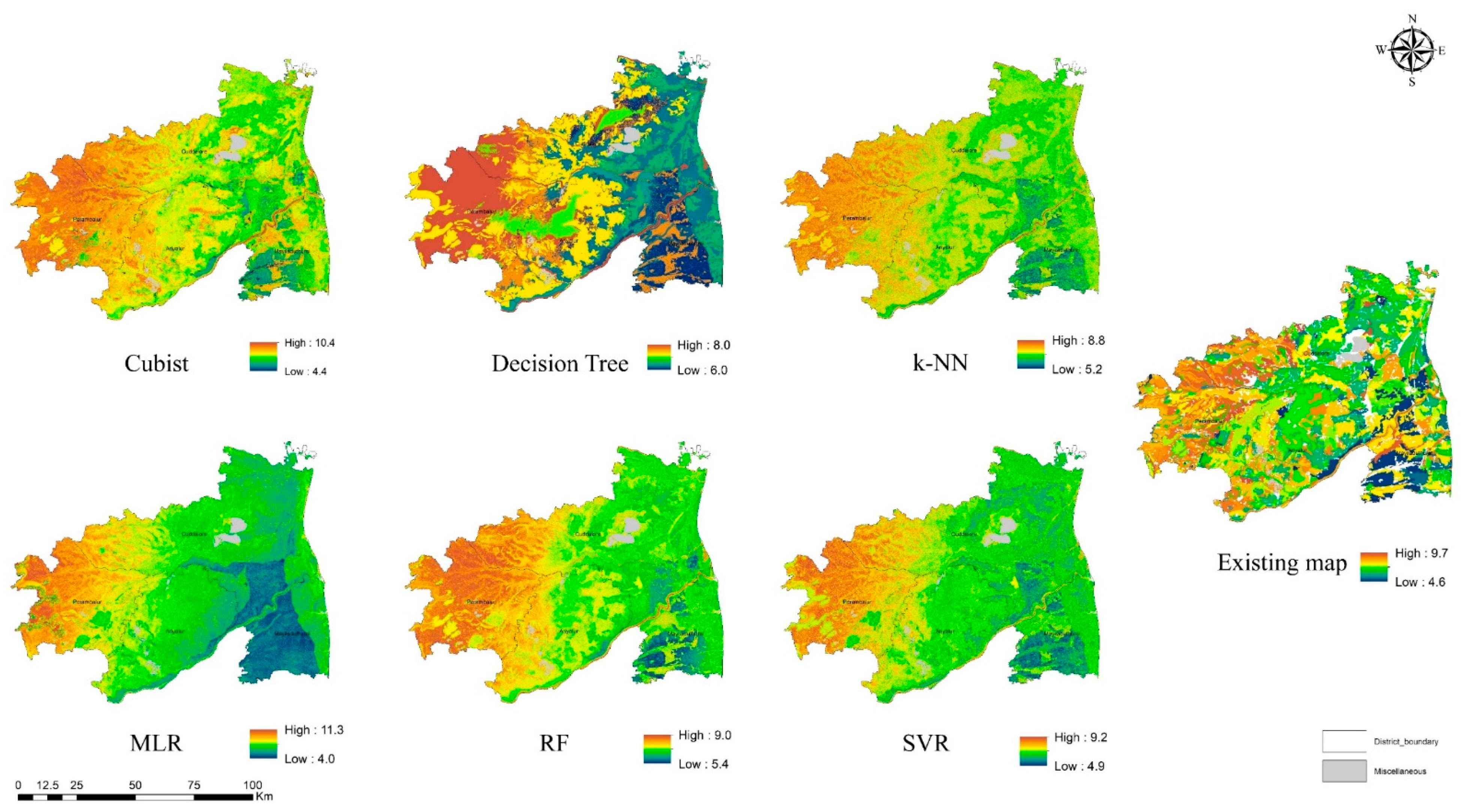
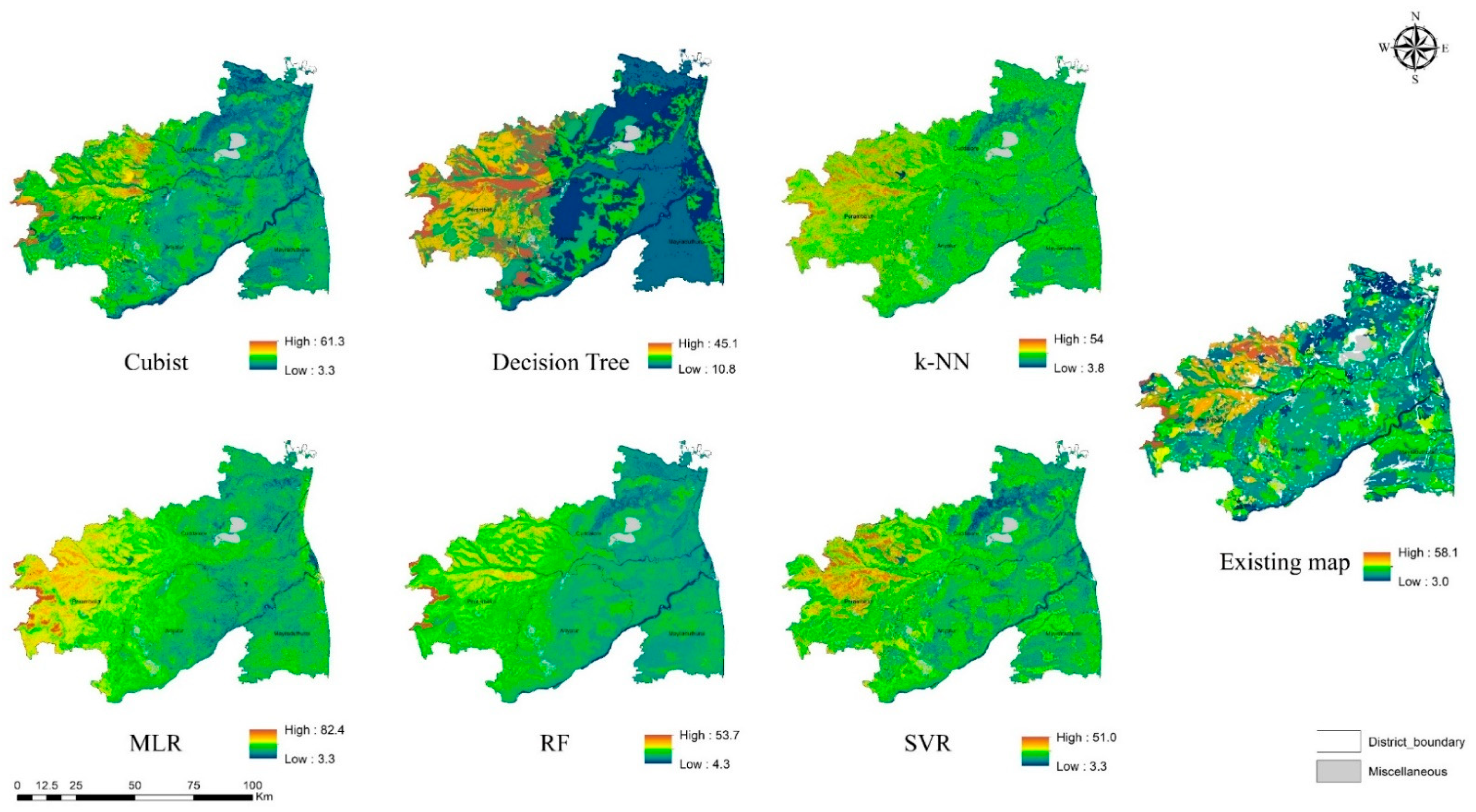
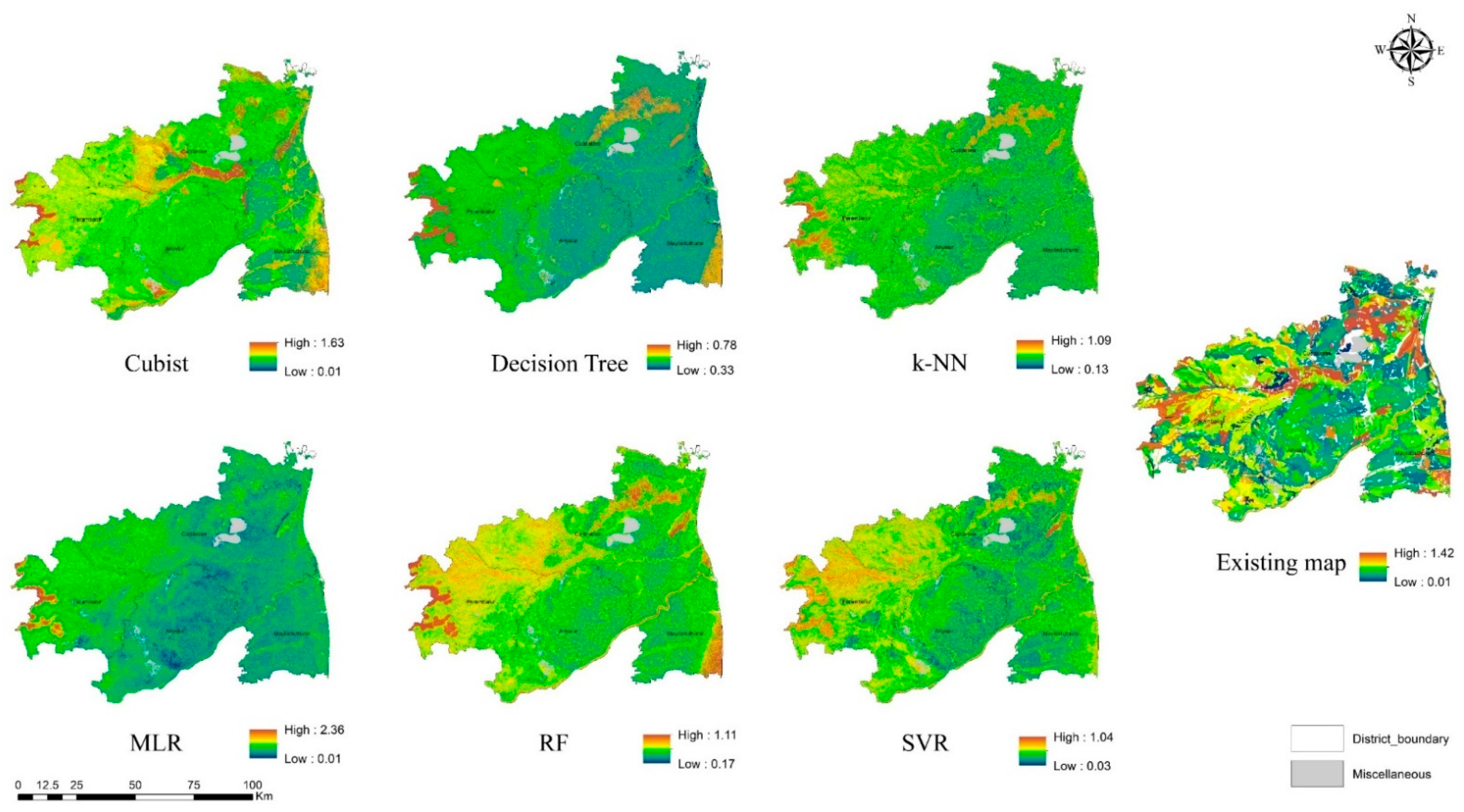
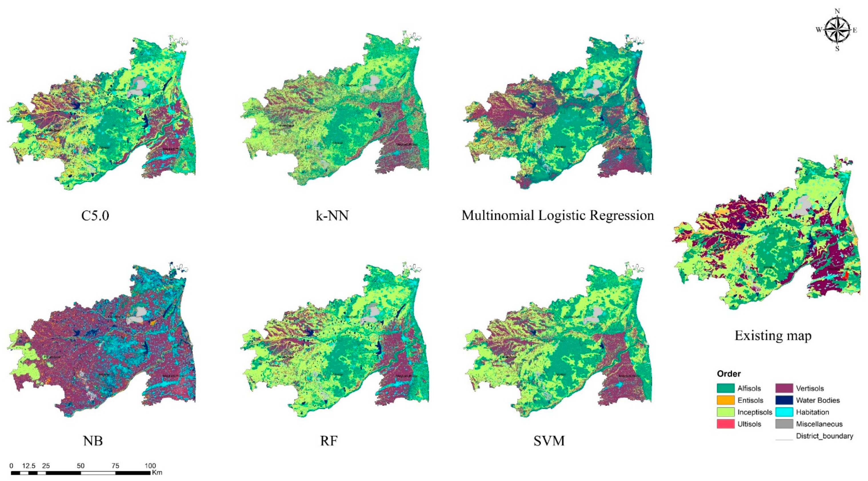
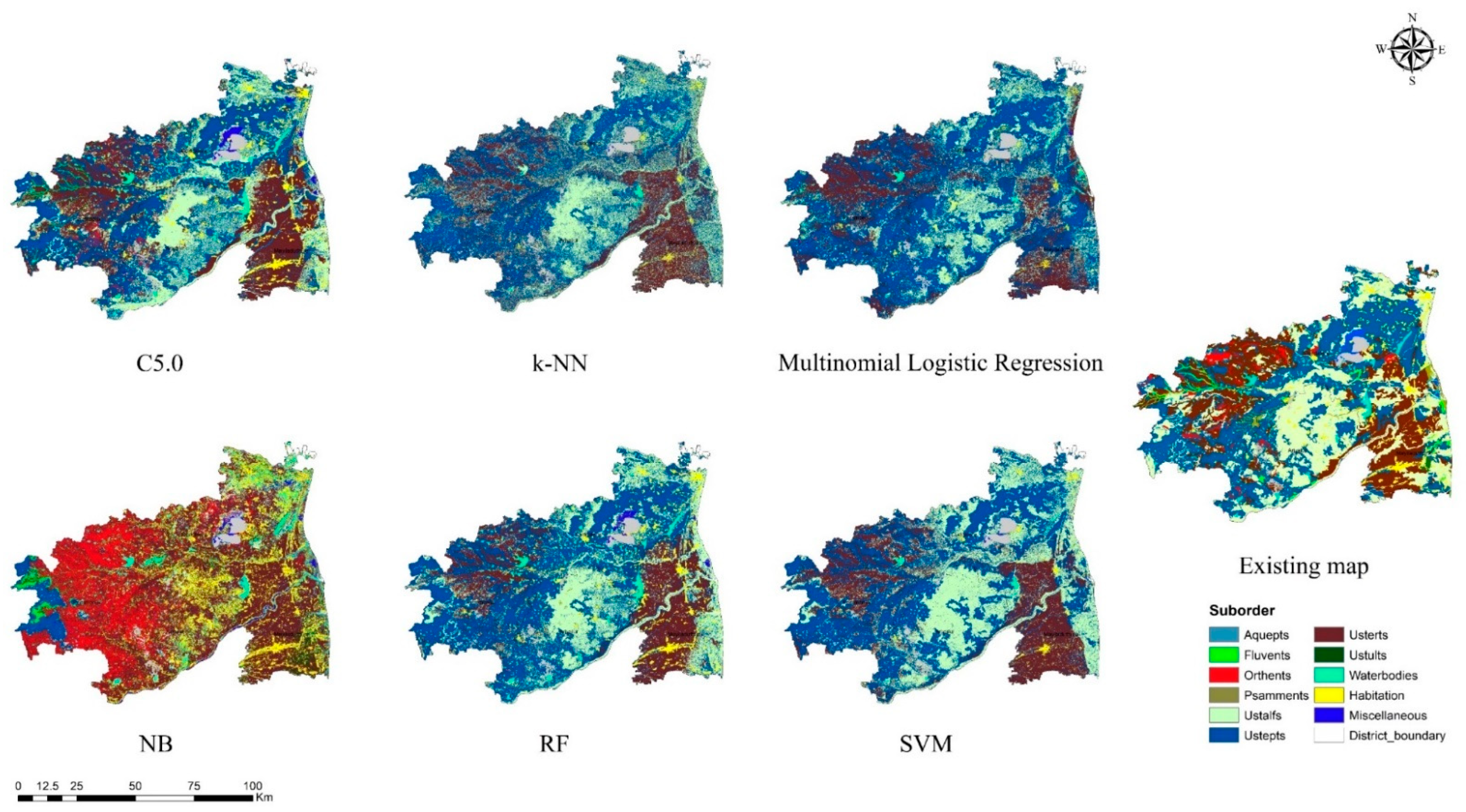
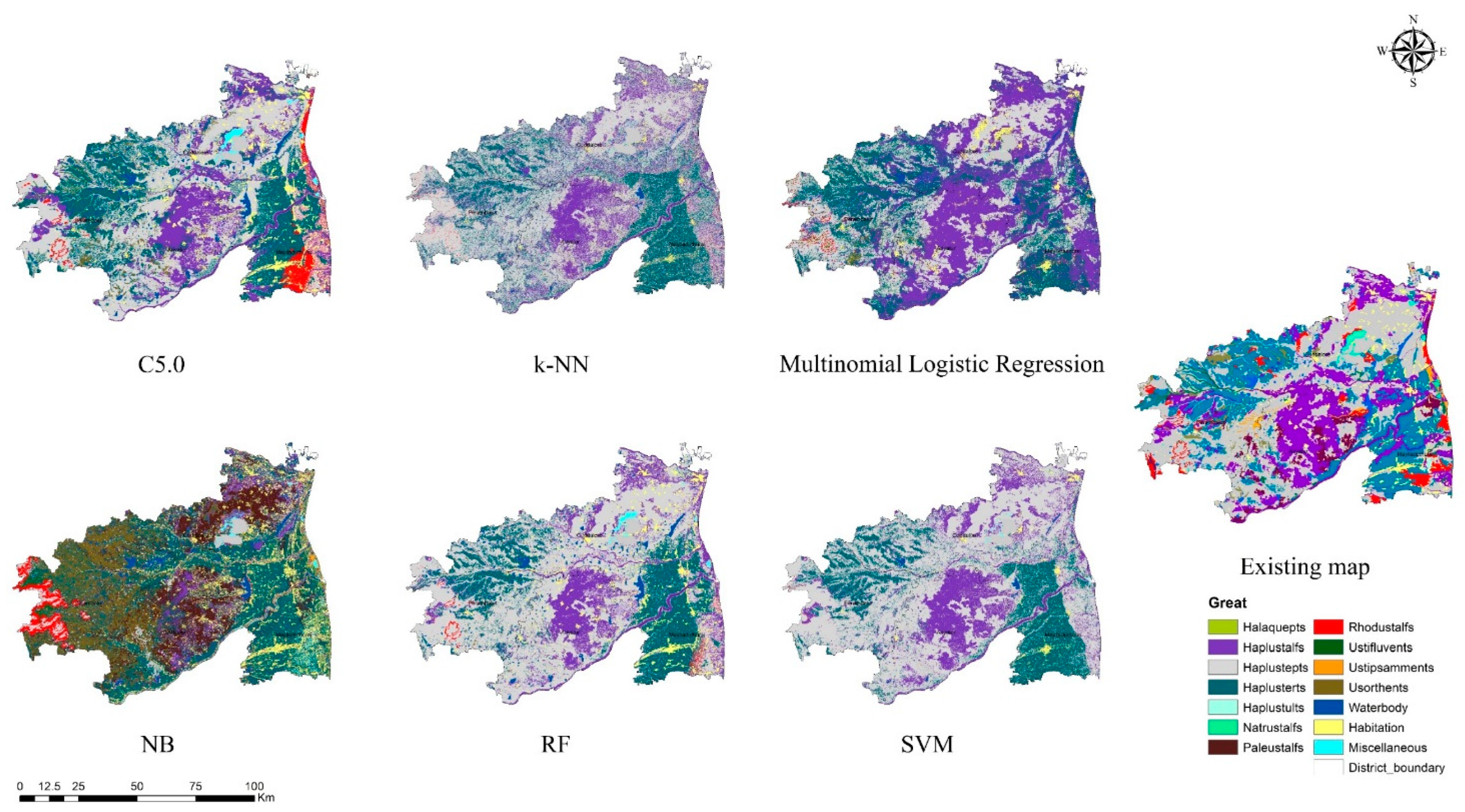
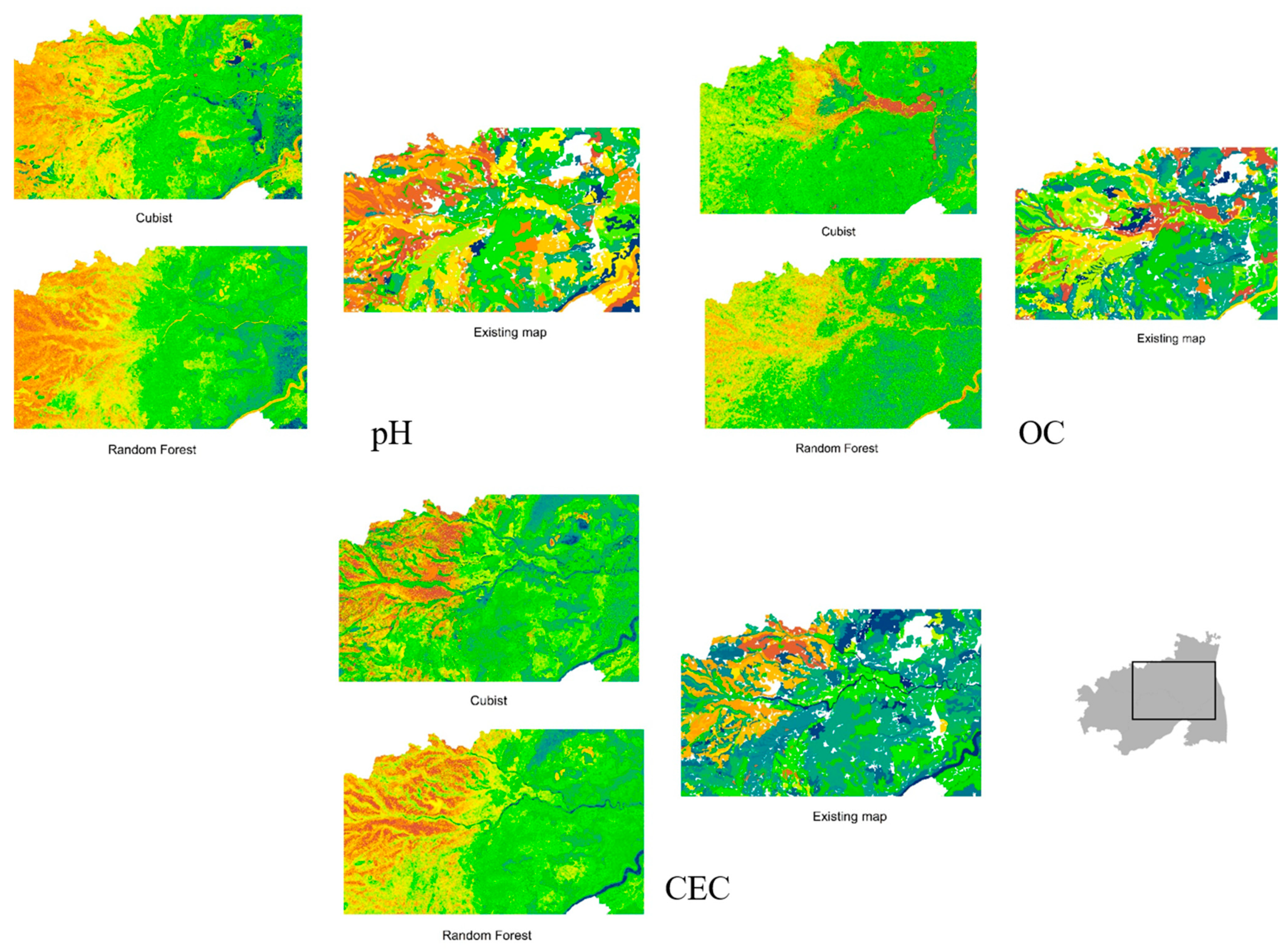
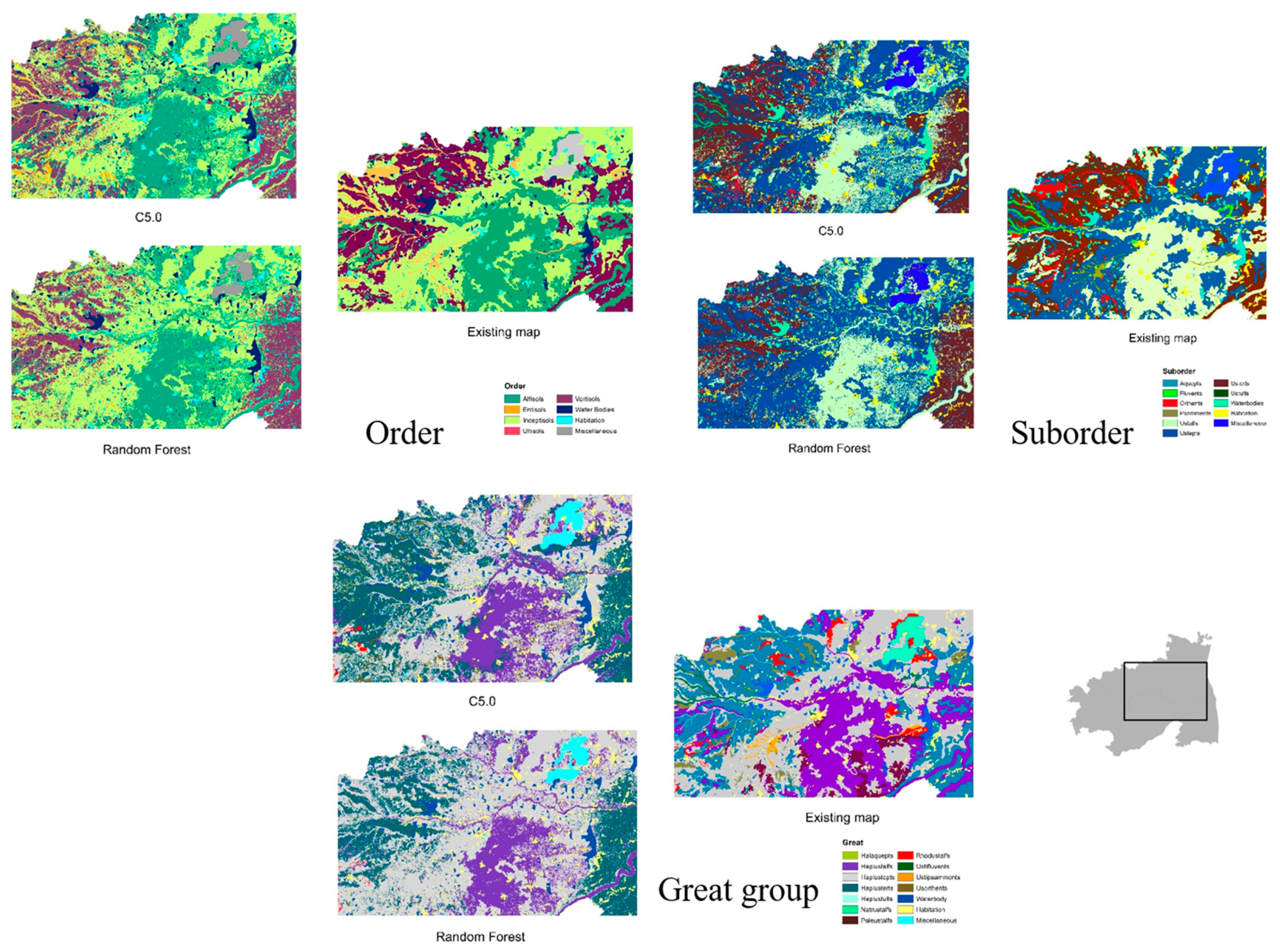
3.3. Visual Assessment

The machine learning algorithms for the spatial modelling and prediction of the quantitative and qualitative soil attributes generated through the raster “predict” function were depicted as their respective attribute maps in Figure 2, Figure 3, Figure 4, Figure 5, Figure 6 and Figure 7. The predicted continuous soil attribute maps were similar to the existing maps, with the added spatial variations explained through the predictions. The comparison of the prediction maps of the pH, OC, and CEC with the existing maps showed that most intricate spatial variations were explained by the Cubist and random forest algorithms, followed by support vector regression, k-NN, decision trees, and multiple linear regression, with an increasing gradient of all soil attributes from west to east. The predicted OC attribute maps depicted a very low concentration, which can be substantiated based on the slope direction, depth, and elevation of the study area.
The lower elevation areas were generally estimated as having lower carbon concentrations due to the increased temperatures [64]. The variations in the minimum and maximum values for the soil attributes were usually attributed to the bias and indicated the underfitting and overfitting of the predictions. The predicted categorical soil attribute maps were almost identical to the existing class maps with variations in the shape and size of the grid clusters, except for the map derived using the naïve Bayes classifier, which depicted evident bias and inconsistencies in the predictions of the implicated categorical soil attributes. In addition, a slight ambiguity in the feature space along the areas of great diversity was also observed for the class prediction maps obtained using multinomial logistic regression and k-NN. Further, the speckled results produced by k-NN due to overfitting might be difficult to interpret.
A larger proportion of the study area was covered by the Inceptisols soil order. The random forest and C5.0-derived soil class maps presented the clearest representation of the class elements followed by SVM, k-NN, and multinomial logistics regression. Although C5.0 and SVM removed three class elements of the great group, they were considered for their potential to adhere to other class elements almost identical to the existing maps. In summary, the predicted soil attribute maps depicted the complex spatial organisation of the variations associated with the existing soil maps and confirmed that all the prediction models, except for naïve Bayes (soil class), could digitally map the soil attributes, but the maps were more accurate with the selected models. The RF and Cubist algorithms for the continuous soil attributes were almost identical to the existing maps, with much greater delineation facilitated by the Cubist algorithm for all the continuous soil attributes considered (Figure 8).
Similarly, when comparing the C5.0 and RF predictions with the existing maps, finer and more detailed boundary delineations were attributed to the C5.0 algorithm (Figure 9). The delineation variations may be attributed to the predictor covariates’ contributions to the spatial model calibration.

3.4. Permutation Feature Importance

The percentage contribution of each parameter derived through PFI analysis was abstracted cumulatively and these are depicted in Table 6.
From Table 6, it can be inferred that the highest overall contributions were from the terrain covariate, which indicates the primary effect of the topographical characteristics on the spatial variability of the soil properties. In general, most models had differing contributions from the parent material and terrain parameters in the model calibration. Between the terrain and parent material covariates, the categorical soil attributes were mostly determined using the terrain parameters. Similarly, the parent material covariate was used the most by the continuous soil attributes. This explains the influence of the nature of the covariate parameter on spatial modelling. Further, MLR showed its linear tendency of data fitting by increasing the incorporation of continuous predictors rather than categorical predictors for its model calibration. Attributable to only two climatic parameters implemented, the influence of the climate covariate on all soil attributes sufficiently explains their importance in predictions of soil properties. The effect of the organisms covariate indicates the constant influence of underlying organisms and other anthropogenic activities on the descriptions of the soil attributes [65].
Furthermore, several of the machine learning algorithms exhibited no influence of the covariates on the calibrated model, which further substantiates the higher bias associated with the models discussed. In summary, for qualitative soil attributes, the Cubist model had an almost equal contribution from all the covariates for its spatial predictions. The equal influence of the covariates is reflected in the finer delineations of the spatial variations accounted for by the Cubist algorithms. Further, impartial influences were presented by the other machine learning algorithms for each soil attribute.
The terrain covariate facilitated a greater influence of the pH soil attribute, followed by the parent material, organisms, and climatic parameters. The influence of the parent material in addition to the terrain attributes can explain the spatial variability of the pH based on the composition of soil-forming materials. The contribution of the organisms covariate was found to be the second highest for the OC after the terrain attributes, which substantiates the generalised influence of the organisms on the soil carbon and organic matter contents. More specifically, the effects of Landsat band 3, LULC, and NDVI on the OC prediction were higher, which has been reported in several studies [66,67]. Similar to those of the OC, the predictions of the CEC showed a stronger influence of organisms than parent material, which contrasts the order of the influence exhibited by the covariates for the pH and CEC soil attributes. In addition, in the cases of the categorical variables, the terrain attributes had a greater influence, followed by parent material and organisms for the C5.0 algorithm. However, the RF algorithm exhibited a contrasting order, with terrain as the most influential, followed by organisms and parent material. Moreover, the inclusion of the parent material in the C5.0 algorithm explains the segregations and almost finer delineations among the classes. This might further substantiate that most soil classifications were based on parent material characteristics [68].

4. Discussion

4.1. Model Efficiency and Performance

Model performance is generally based on the nature of the datasets implicated; the parameters depicted; and the complexity, consistency, and structure of the model proposed [69]. Based on the evaluation metrics assessed for the soil attributes, discussions are herein presented for the comparison of the machine learning algorithms. Besides the metrics specified, the selections were also made by comparing the quality of the visual delineations provided by a particular machine learning algorithm. Since a standardised measure of model efficiency has not yet been determined, several evaluation metrics were assessed to capture the variations in the model training. In general, the comparison results and the resulting predictions of the study might vary from other studies. Although speculating about the reasons behind the differences is difficult, the differences could be because of the varying nature of the study area and the quantity and quality of the soil attributes.

4.1.1. Quantitative Soil Attributes

In general, the lower R2 and CCC values presented by the algorithms were due to the higher variability and complex interactions depicted by the environmental covariates. The high variability can be explained by the management practices, vegetation, and climatic factors influencing the characteristics of the study area [70]. Furthermore, several studies indicated a similar range of R2 results, stating that R2 values < 0.50 are common [71], considering the spatial prediction of the continuous soil attributes. Previous studies on continuous spatial soil predictions resulted in R2 ranges not exceeding 70% [72,73,74,75,76,77].
Other research on digital soil mapping of the continuous soil attributes in India presented similar spatial soil predictions in the watershed regions of Karnataka, India. The R2 values of the predictions for the pH, EC, and OC using random forest regression (RF) yielded 46%, 16%, and 19%, respectively, for the Aland watershed and 30%, 7%, and 12% for the Guppi watershed [78]. Recent works evaluating digital soil-mapping approaches indicated that the variations exhibited by the R2 measure ranged from 9% to 48% for predicting soil fertility nutrients [79]. The low R2 values were due to the lower range of the soil attributes and non-significant spatial variations of the inputted soil datasets. The differences in the results of the evaluation metrics due to scale and range have also been investigated in other studies [80] and it has been stated that the lower values might indicate the insufficiency of the covariates to explain the soil attributes aside from their range and scale [81].
The lower RMSE measure indicates the reasonable performance of the spatial prediction models, which was expected using the sampled data. Further, when comparing the bias, the pH and OC attributes provided an unbiased prediction, with k-NN and MLR suffering a moderate bias when predicting the CEC attribute. When comparing the evaluation metrics derived using the test datasets, for the spatial prediction of the continuous soil attributes, the RF model consistently made the most accurate predictions (with the highest R2 and lowest RMSE). Furthermore, the Cubist model also performed efficiently in addition to the RF algorithm. Similar results were found in previous studies [76,77,78,79,80,81,82,83], which stated the RF and Cubist algorithms as being among the most efficient soil organic carbon prediction models. However, these studies showed differences in the R2 and other evaluation metrics, which might be due to the different sampling designs, scales, and ranges of the soil attributes and covariates incorporated.
Several studies indicated that the random forest approach was considered suitable for spatial soil predictions because of its ability to handle many covariates, limited samples, and low need for hyperparameter tweaking [84]. Furthermore, following RF and Cubist, regression trees (DT) reported comparable prediction metrics. The lower accuracy of support vector machine can be attributed to the larger sampling data implemented. Thus, based on the evaluation metrics and visual assessments, among the machine learning algorithms compared, the RF and Cubist are considered efficient models for predicting the spatial variations in the pH, OC, and CEC for the proposed study.

4.1.2. Qualitative Soil Attributes

The evaluation metrics assessed for the qualitative soil attributes indicated that all the prediction models performed sufficiently in explaining the variability of the soil attributes, except for multinomial logistic regression and the naïve Bayes classifier. In addition to estimating the kappa and overall accuracy (OA), disagreement measures adopted in several recent studies were also estimated in the comparison of the machine learning algorithms for their robustness in depicting the variations in the predicted class [85,86,87,88,89].
Based on the evaluation metrics assessed, the random forest and C5.0 algorithm outperformed other models and predominantly reported the most accurate results for every soil class prediction implicated. Previous studies found that the RF [85,90] and C5.0 [91] algorithms provided the most accurate results and similar results were found by Zeraatpisheh et al. [92], which resulted in multinomial logistic regression for higher soil taxonomic units (due to the inclusion of the AIC-based predictor variable selection) and RF for lower taxonomic units as the best-performing models. Other studies [93] also resulted in RF (kappa = 0.55) being a more efficient model than multinomial logistic regression (kappa = 0.33). The prediction of soil class units in Iran also reported similar results [94], with the RF model performing the best at higher taxonomical units with OAs of 0.87 and 0.52 and kappas of 0.57 and 0.38 for order and suborder class predictions, respectively. The study also reported the increased prediction accuracy of RF compared to the proposed ensemble model.
The overall accuracies of the DSM maps selected based on the evaluation metrics for each soil taxonomic level ranged from 65% to 67%, which was the recommended level reported in the previous studies [95,96]. The results obtained were generally found to be comparable to or higher than the previous studies. For example, soil class prediction [89] in Brazil resulted in an overall accuracy of 0.54 for the RF algorithm. Similar results to our study area have been reported for predicting soil class units, with overall accuracies of 68%, 63.6%, and 58.8% achieved through RF, classification trees, and multinomial logistic regression, respectively [97].
When comparing the disagreement components between the algorithms, the validated naïve Bayes classifier had a higher number of disagreements. The total disagreement measure was found to be the lowest for the RF and C5.0 algorithms, with a higher allocation disagreement. The major limitation of the soil class prediction associated with the C5.0 and support vector machine was that the fitted model failed to classify some of the soil classes, which was mainly attributed to low sampling frequencies related to the particular soil class element. In general, classes with lower sampling frequencies were predicted less accurately due to the limited observations associated with segregating such classes in the feature space.
Further, it was evident that the increase in the number of class categories had no significant effect on the resulting prediction accuracies. From the assessment of the percentage contributions of the covariates, it was observed that NB and multinomial logistic regression did not consider the parent material covariates (spectral ratios). Although the RF and C5.0 algorithms provided comparable results in observing the evaluation metrics, based on the visual assessments, all the machine learning algorithms derived a comparable interpretation, except for the NB classifier.

4.2. Potential Applications at the Farm Level and Policy Decisions

Climate change and an increasing population demand a well-established soil database to increase productivity, reduce emissions, and create a safe environment for future food security. Soil databases are used to assess soil conditions to mitigate global concerns regarding environmental sustainability. In DSM, several studies have addressed the spatial prediction of the contiguous soil attributes viz. pH, CEC, organic carbon, etc., compared to the categorical attributes [98]. The block-level soil information with legacy soil maps also lacks detailed soil information, whereas the soil information predicted and downscaled through DSM helps farmers with their day-to-day management decisions [99]. The high-resolution digital maps can be used to assess crop suitability, soil and land management practices, site-specific fertilizer recommendations, the integration of spatial variability in VRT systems, and irrigation scheduling, subsequently reducing operational costs by optimising the inputs. The proper selection of crops, effective soil and land management practices, and balanced fertilization using DSM will result in reduced input costs and increased farm outputs, thereby improving the net income of farmers in addition to ensuring their livelihoods through crop cultivation [100].
The results from this study depict the strength of digital soil-mapping techniques to generate precise information pertaining to soils. The knowledge can be transferred to farmers through mobile applications and other Information and Communication Technology (ICT) tools on digital platforms. Agro-technology transfer has reached most smallholder farmers in Tamil Nadu, which account for nine million farm holdings, with large variability in the spatial attributes of soil. The further development of soil-based ICT tools in local languages will empower farmers in terms of farm management, resource recycling, and adopting strategies to manage soil constraints [101]. The technology has the potential for upscaling across the different geographies of India.

5. Conclusions

The current study was based on the soil information derived from the existing soil maps, which were based on the stratified random sampling procedure. From the class prediction results, it can be inferred that the strata-based sampling procedure may limit the depiction of the transition variations near the strata boundaries. The effect of the nature and range of the soil and predictor variables had a considerable influence on the resulting predictions. Irrespective of the number of covariates considered, it was observed that the continuous scale predictors had a comparably greater influence than the categorical predictor variables on the model calibration, except for NB and multinomial logistic regression. The key findings of our research are:
  • From the suite of machine learning algorithms compared for mapping three continuous soil attributes and three soil taxonomical units, it can be inferred from the visual interpretation that all the algorithms provided a reasonable spatial prediction of the soil attributes, except for the NB classifier.
  • Among the ML models, the tree-based ensemble (RF) and rule-based models (Cubist and C5.0) efficiently predicted the soil properties spatially. The efficiency of the models can be further increased by adopting appropriate sampling and tuning methods.
  • The probability-based machine learning algorithms (NB and multinomial logistic regression) produced biased and crude results, which might have been due to the inclusion of continuous covariate predictors for the model calibration. Hence, the transformation of covariate predictors and the implementation of suitable variable selection techniques can improve the accuracy of the predictions.
  • The results of k-NN, SVM, and SVR with default parameterisation were used to deduce the potential of the models, which was further increased by the appropriate tuning of parameters. The time required for the computation of SVM/SVR parameterisation is tedious for a larger dataset; hence, it is recommended for limited observations at a smaller scale.
This study also revealed that the spatial predictions of the soil attributes at regional levels with contrasting climates and landscapes were substantial. The tree-based models can be further enhanced and utilised for spatial predictions for producing digital soil maps at other regional and state levels. The digital soil maps generated at the higher spatial resolution will help farmers to execute effective farm planning through the choice of efficient crops, the scientific scheduling of irrigation and need-based nutrient application, effective management practices in the case of soil constraints, and the facilitation of the transformation to digital agriculture.

Author Contributions

Conceptualization, R.K. (Ramalingam Kumaraperumal) and S.P.; Data curation, M.N.R., V.S., A.M.N. and T.V.T.K.; Formal analysis, R.K. (Ramalingam Kumaraperumal), S.P., V.G., R.K. (Ragunath Kaliaperumal) and M.N.R.; Funding acquisition, S.P. and M.K.Y.; Investigation, D.M. and M.N.R.; Methodology, R.K. (Ramalingam Kumaraperumal), S.P., V.G. and M.N.R.; Project administration, S.P. and M.K.Y.; Resources, R.K. (Ramalingam Kumaraperumal), R.K. (Ragunath Kaliaperumal) and D.M.; Software, M.N.R., V.S., A.M.N. and T.V.T.K.; Supervision, R.K. (Ramalingam Kumaraperumal), S.P., V.G. and R.K. (Ragunath Kaliaperumal); Validation, M.N.R., A.M.N. and D.M.; Visualization, M.N.R. and V.S.; Writing—original draft, R.K. (Ramalingam Kumaraperumal) and S.P.; Writing—review and editing, M.N.R., V.S., A.M.N., T.V.T.K. and R.K. (Ramalingam Kumaraperumal). All authors have read and agreed to the published version of the manuscript.

Funding

This research and the APC were funded by GIZ, Germany, Deutsche Gesellschaft für Internationale Zusammenarbeit (Grant number 81278637).

Institutional Review Board Statement

Not applicable.

Informed Consent Statement

Not applicable.

Data Availability Statement

Not applicable.

Acknowledgments

This work is part of the GIZ-ICRI Project for the generation of digital soil maps for Tamil Nadu. Legacy soil data and environmental covariates were obtained from various sources; hence, the authors thank all of them for providing their resources. The boundaries, colours, denominations, and other information shown on any map in this work do not imply any judgment on the part of the authors or their institutes concerning the legal status of any territory or the endorsement or acceptance of such boundaries.

Conflicts of Interest

The authors declare no conflict of interest.

References

  1. Dash, P.K.; Panigrahi, N.; Mishra, A. Identifying opportunities to improve digital soil mapping in India: A systematic review. Geoderma Reg. 2021, 28, e00478. [Google Scholar] [CrossRef]
  2. Zhu, A.-X.; Hudson, B.; Burt, J.; Lubich, K.; Simonson, D. Soil mapping using GIS, expert knowledge, and fuzzy logic. Soil Sci. Soc. Am. J. 2001, 65, 1463–1472. [Google Scholar] [CrossRef] [Green Version]
  3. Bui, E.N.; Searle, R.D.; Wilson, P.R.; Philip, S.R.; Thomas, M.; Brough, D.; Harms, B.; Hill, J.V.; Holmes, K.; Smolinski, H.J. Soil surveyor knowledge in digital soil mapping and assessment in Australia. Geoderma Reg. 2020, 22, e00299. [Google Scholar] [CrossRef]
  4. Dharumarajan, S.; Hegde, R.; Singh, S.K. Spatial prediction of major soil properties using Random Forest techniques—A case study in semi-arid tropics of South India. Geoderma Reg. 2017, 10, 154–162. [Google Scholar] [CrossRef]
  5. Zhang, G.-l.; Feng, L.; Song, X.-d. Recent progress and future prospect of digital soil mapping: A review. J. Integr. Agric. 2017, 16, 2871–2885. [Google Scholar] [CrossRef]
  6. Lagacherie, P.; McBratney, A. Spatial soil information systems and spatial soil inference systems: Perspectives for digital soil mapping. Dev. Soil Sci. 2006, 31, 3–22. [Google Scholar]
  7. Minasny, B.; McBratney, A.B. Digital soil mapping: A brief history and some lessons. Geoderma 2016, 264, 301–311. [Google Scholar] [CrossRef]
  8. Zeraatpisheh, M.; Jafari, A.; Bodaghabadi, M.B.; Ayoubi, S.; Taghizadeh-Mehrjardi, R.; Toomanian, N.; Kerry, R.; Xu, M. Conventional and digital soil mapping in Iran: Past, present, and future. Catena 2020, 188, 104424. [Google Scholar] [CrossRef]
  9. Song, Y.-Q.; Yang, L.-A.; Li, B.; Hu, Y.-M.; Wang, A.-L.; Zhou, W.; Cui, X.-S.; Liu, Y.-L. Spatial prediction of soil organic matter using a hybrid geostatistical model of an extreme learning machine and ordinary kriging. Sustainability 2017, 9, 754. [Google Scholar] [CrossRef] [Green Version]
  10. Wiesmeier, M.; Barthold, F.; Blank, B.; Kögel-Knabner, I. Digital mapping of soil organic matter stocks using Random Forest modeling in a semi-arid steppe ecosystem. Plant Soil 2011, 340, 7–24. [Google Scholar] [CrossRef]
  11. Dharumarajan, S.; Hegde, R. Digital mapping of soil texture classes using Random Forest classification algorithm. Soil Use Manag. 2020, 38, 135–149. [Google Scholar] [CrossRef]
  12. Vaysse, K.; Lagacherie, P. Using quantile regression forest to estimate uncertainty of digital soil mapping products. Geoderma 2017, 291, 55–64. [Google Scholar] [CrossRef]
  13. Dharumarajan, S.; Vasundhara, R.; Suputhra, A.; Lalitha, M.; Hegde, R. Prediction of soil depth in Karnataka using digital soil mapping approach. J. Indian Soc. Remote Sens. 2020, 48, 1593–1600. [Google Scholar] [CrossRef]
  14. Rossel, R.A.V.; Behrens, T. Using data mining to model and interpret soil diffuse reflectance spectra. Geoderma 2010, 158, 46–54. [Google Scholar] [CrossRef]
  15. Maynard, J.J.; Levi, M.R. Hyper-temporal remote sensing for digital soil mapping: Characterizing soil-vegetation response to climatic variability. Geoderma 2017, 285, 94–109. [Google Scholar] [CrossRef] [Green Version]
  16. Taalab, K.; Corstanje, R.; Zawadzka, J.; Mayr, T.; Whelan, M.J.; Hannam, J.A.; Creamer, R. On the application of Bayesian Networks in Digital Soil Mapping. Geoderma 2015, 259–260, 134–148. [Google Scholar] [CrossRef]
  17. Freire, S.; de Lisboa, N.; Fonseca, I.; Brasil, R.; Rocha, J.; Tenedório, J.A. Using artificial neural networks for digital soil mapping—A comparison of MLP and SOM approaches. In Proceedings of the AGILE, Nashville, TN, USA, 5–9 August 2013. [Google Scholar]
  18. Mulder, V.L.; Lacoste, M.; Richer-de-Forges, A.C.; Martin, M.P.; Arrouays, D. National versus global modelling the 3D distribution of soil organic carbon in mainland France. Geoderma 2016, 263, 16–34. [Google Scholar] [CrossRef]
  19. Malone, B.P.; Minasny, B.; McBratney, A.B. Categorical soil attribute modeling and mapping. In Using R for Digital Soil Mapping; Springer: Berlin/Heidelberg, Germany, 2017; pp. 151–167. [Google Scholar]
  20. Zhang, Y.; Ji, W.; Saurette, D.D.; Easher, T.H.; Li, H.; Shi, Z.; Adamchuk, V.I.; Biswas, A. Three-dimensional digital soil mapping of multiple soil properties at a field-scale using regression kriging. Geoderma 2020, 366, 114253. [Google Scholar] [CrossRef]
  21. Padarian, J.; Minasny, B.; McBratney, A.B. Using deep learning for digital soil mapping. Soil 2019, 5, 79–89. [Google Scholar] [CrossRef] [Green Version]
  22. Wadoux, A.M.-C.; Padarian, J.; Minasny, B. Multi-source data integration for soil mapping using deep learning. Soil 2019, 5, 107–119. [Google Scholar] [CrossRef] [Green Version]
  23. Kalambukattu, J.G.; Kumar, S.; Arya Raj, R. Digital soil mapping in a Himalayan watershed using remote sensing and terrain parameters employing artificial neural network model. Environ. Earth Sci. 2018, 77, 203. [Google Scholar] [CrossRef]
  24. Chang, C.-W.; Laird, D.A.; Mausbach, M.J.; Hurburgh, C.R. Near-infrared reflectance spectroscopy–principal components regression analyses of soil properties. Soil Sci. Soc. Am. J. 2001, 65, 480–490. [Google Scholar] [CrossRef] [Green Version]
  25. Yang, R.-M.; Zhang, G.-L.; Liu, F.; Lu, Y.-Y.; Yang, F.; Yang, F.; Yang, M.; Zhao, Y.-G.; Li, D.-C. Comparison of boosted regression tree and random forest models for mapping topsoil organic carbon concentration in an alpine ecosystem. Ecol. Indic. 2016, 60, 870–878. [Google Scholar] [CrossRef]
  26. Wang, B.; Waters, C.; Orgill, S.; Gray, J.; Cowie, A.; Clark, A.; Li Liu, D. High resolution mapping of soil organic carbon stocks using remote sensing variables in the semi-arid rangelands of eastern Australia. Sci. Total Environ. 2018, 630, 367–378. [Google Scholar] [CrossRef] [PubMed]
  27. Brungard, C.; Nauman, T.; Duniway, M.; Veblen, K.; Nehring, K.; White, D.; Salley, S.; Anchang, J. Regional ensemble modeling reduces uncertainty for digital soil mapping. Geoderma 2021, 397, 114998. [Google Scholar] [CrossRef]
  28. Pahlavan-Rad, M.R.; Khormali, F.; Toomanian, N.; Brungard, C.W.; Kiani, F.; Komaki, C.B.; Bogaert, P. Legacy soil maps as a covariate in digital soil mapping: A case study from Northern Iran. Geoderma 2016, 279, 141–148. [Google Scholar] [CrossRef]
  29. Kaya, F.; Başayiğit, L. Spatial Prediction and Digital Mapping of Soil Texture Classes in a Floodplain Using Multinomial Logistic Regression. In Proceedings of the International Conference on Intelligent and Fuzzy Systems, Istanbul, Turkey, 24–26 August 2021; pp. 463–473. [Google Scholar]
  30. Mansuy, N.; Thiffault, E.; Paré, D.; Bernier, P.; Guindon, L.; Villemaire, P.; Poirier, V.; Beaudoin, A. Digital mapping of soil properties in Canadian managed forests at 250m of resolution using the k-nearest neighbor method. Geoderma 2014, 235–236, 59–73. [Google Scholar] [CrossRef]
  31. Khaledian, Y.; Miller, B.A. Selecting appropriate machine learning methods for digital soil mapping. Appl. Math. Model. 2020, 81, 401–418. [Google Scholar] [CrossRef]
  32. Casalicchio, G.; Molnar, C.; Bischl, B. Visualizing the feature importance for black box models. In Proceedings of the Joint European Conference on Machine Learning and Knowledge Discovery in Databases, Dublin, Ireland, 10–14 September 2018; pp. 655–670. [Google Scholar]
  33. NRIS. Manual of National Wastelands Monitoring Using Multitemporal Satellite Data; National Remote Sensing Agency, Department of Space, Government of India: New Delhi, India, 2007; p. 98.
  34. NRSC. Land Use/Land Cover Database on 1:50,000 Scale, Natural Resources Census Project, LUCMD, LRUMG, RSAA; National Remote Sensing Centre, ISRO: Hyderabad, India, 2016.
  35. NRSC. Lithology, Physiography and Soils of Tamil Nadu at 1:50,000 Scale, Natural Resources Census Project; National Remote Sensing Centre, ISRO in Collaboration with Institute of Remote Sensing and Tamil Nadu Agricultural University: Hyderabad, India, 2012.
  36. Hastie, T.; Tibshirani, R.; Friedman, J.H. The Elements of Statistical Learning: Data Mining, Inference, and Prediction; Springer: Berlin/Heidelberg, Germany, 2009; Volume 2. [Google Scholar]
  37. Ripley, B.; Venables, W.; Ripley, M.B. Package ‘nnet’. R Package Version 2016, 7, 700. [Google Scholar]
  38. Kuhn, M. Building predictive models in R using the caret package. J. Stat. Softw. 2008, 28, 1–26. [Google Scholar] [CrossRef] [Green Version]
  39. Therneau, T.; Atkinson, B.; Ripley, B.; Ripley, M.B. Package ‘rpart’. R Package Version 4.1.19. Available online: cran.ma.ic.ac.uk/web/packages/rpart/rpart.pdf (accessed on 23 June 2021).
  40. Kuhn, M.; Quinlan, R. C50: C5.0 Decision Trees and Rule-Based Models. CRAN UTC. Available online: https://cran.r-project.org/web/packages/C50/C50.pdf (accessed on 23 June 2021).
  41. Meyer, D.; Dimitriadou, E.; Hornik, K.; Weingessel, A.; Leisch, F. e1071: Misc Functions of the Department of Statistics, Probability Theory Group. (Formerly: E1071), TU Wien [R Package Version 1.7-12]. Available online: https://cran.r-project.org/web/packages/e1071/e1071.pdf (accessed on 23 June 2021).
  42. Kuhn, M.; Weston, S.; Keefer, C.; Kuhn, M.M. Package ‘Cubist’. Rule- and Instance-Based Regression Modeling. R Package Version 0.4.1. Available online: https://cran.r-project.org/web/packages/Cubist/Cubist.pdf (accessed on 23 June 2021).
  43. Liaw, A.; Wiener, M. Classification and Regression by randomForest. R News 2002, 2, 18–22. [Google Scholar]
  44. James, G.; Witten, D.; Hastie, T.; Tibshirani, R. An Introduction to Statistical Learning; Springer: Berlin/Heidelberg, Germany, 2013; Volume 112. [Google Scholar]
  45. Jafari, A.; Finke, P.; Vande Wauw, J.; Ayoubi, S.; Khademi, H. Spatial prediction of USDA-great soil groups in the arid Zarand region, Iran: Comparing logistic regression approaches to predict diagnostic horizons and soil types. Eur. J. Soil Sci. 2012, 63, 284–298. [Google Scholar] [CrossRef]
  46. Kempen, B.; Brus, D.J.; Heuvelink, G.B.; Stoorvogel, J.J. Updating the 1: 50,000 Dutch soil map using legacy soil data: A multinomial logistic regression approach. Geoderma 2009, 151, 311–326. [Google Scholar] [CrossRef]
  47. Zhang, L.; Yang, L.; Ma, T.; Shen, F.; Cai, Y.; Zhou, C. A self-training semi-supervised machine learning method for predictive mapping of soil classes with limited sample data. Geoderma 2021, 384, 114809. [Google Scholar] [CrossRef]
  48. Cover, T.; Hart, P. Nearest neighbor pattern classification. IEEE Trans. Inf. Theory 1967, 13, 21–27. [Google Scholar] [CrossRef] [Green Version]
  49. Kuhn, M.; Johnson, K. Applied Predictive Modeling; Springer: Berlin/Heidelberg, Germany, 2013; Volume 26. [Google Scholar]
  50. Therneau, T.M.; Atkinson, E.J. An Introduction to Recursive Partitioning Using the RPART Routines; Mayo Foundation: Scottsdale, AZ, USA, 2019; p. 60. [Google Scholar]
  51. Quinlan, J.R. C4. 5: Programming for machine learning. Morgan Kauffmann 1993, 38, 49. [Google Scholar]
  52. Leung, K.M. Naive bayesian classifier. Polytech. Univ. Dep. Comput. Sci./Financ. Risk Eng. 2007, 2007, 123–156. [Google Scholar]
  53. Lamichhane, S.; Kumar, L.; Wilson, B. Digital soil mapping algorithms and covariates for soil organic carbon mapping and their implications: A review. Geoderma 2019, 352, 395–413. [Google Scholar] [CrossRef]
  54. Zhang, M.; Shi, W. Systematic comparison of five machine-learning methods in classification and interpolation of soil particle size fractions using different transformed data. Hydrol. Earth Syst. Sci. Discuss. 2019, 24, 1–39. [Google Scholar]
  55. Quinlan, J.R. Learning with continuous classes. In Proceedings of the 5th Australian Joint Conference on Artificial Intelligence, Hobart, Tasmania, 16–18 November 1992; pp. 343–348. [Google Scholar]
  56. Breiman, L. Random forests. Mach. Learn. 2001, 45, 5–32. [Google Scholar] [CrossRef] [Green Version]
  57. Grimm, R.; Behrens, T.; Märker, M.; Elsenbeer, H. Soil organic carbon concentrations and stocks on Barro Colorado Island—Digital soil mapping using Random Forests analysis. Geoderma 2008, 146, 102–113. [Google Scholar] [CrossRef]
  58. Congalton, R.G. A review of assessing the accuracy of classifications of remotely sensed data. Remote Sens. Environ. 1991, 37, 35–46. [Google Scholar] [CrossRef]
  59. Pontius, R.G.; Millones, M. Death to Kappa: Birth of quantity disagreement and allocation disagreement for accuracy assessment. Int. J. Remote Sens. 2011, 32, 4407–4429. [Google Scholar] [CrossRef]
  60. Fisher, A.; Rudin, C.; Dominici, F. All Models are Wrong, but Many are Useful: Learning a Variable’s Importance by Studying an Entire Class of Prediction Models Simultaneously. J. Mach. Learn. Res. 2019, 20, 177. [Google Scholar] [PubMed]
  61. Molnar, C. Interpretable Machine Learning: A Guide for Making Black Box Models Explainable. 2020. Available online: https://christophm.github.io/interpretable-ml-book/ (accessed on 23 June 2021).
  62. Taghizadeh-Mehrjardi, R.; Hamzehpour, N.; Hassanzadeh, M.; Heung, B.; Goydaragh, M.G.; Schmidt, K.; Scholten, T. Enhancing the accuracy of machine learning models using the super learner technique in digital soil mapping. Geoderma 2021, 399, 115108. [Google Scholar] [CrossRef]
  63. Holmes, K.W.; Kyriakidis, P.C.; Chadwick, O.A.; Soares, J.V.; Roberts, D.A. Multi-scale variability in tropical soil nutrients following land-cover change. Biogeochemistry 2005, 74, 173–203. [Google Scholar] [CrossRef]
  64. Were, K.; Bui, D.T.; Dick, Ø.B.; Singh, B.R. A comparative assessment of support vector regression, artificial neural networks, and random forests for predicting and mapping soil organic carbon stocks across an Afromontane landscape. Ecol. Indic. 2015, 52, 394–403. [Google Scholar] [CrossRef]
  65. McBratney, A.B.; Santos, M.M.; Minasny, B. On digital soil mapping. Geoderma 2003, 117, 3–52. [Google Scholar] [CrossRef]
  66. Mishra, U.; Lal, R.; Slater, B.; Calhoun, F.; Liu, D.; Van Meirvenne, M. Predicting soil organic carbon stock using profile depth distribution functions and ordinary kriging. Soil Sci. Soc. Am. J. 2009, 73, 614–621. [Google Scholar] [CrossRef] [Green Version]
  67. Minasny, B.; McBratney, A.B.; Malone, B.P.; Wheeler, I. Digital mapping of soil carbon. Adv. Agron. 2013, 118, 1–47. [Google Scholar]
  68. Bockheim, J.; Gennadiyev, A.; Hartemink, A.; Brevik, E. Soil-forming factors and Soil Taxonomy. Geoderma 2014, 226–227, 231–237. [Google Scholar] [CrossRef]
  69. Purushothaman, N.K.; Reddy, N.N.; Das, B.S. National-scale maps for soil aggregate size distribution parameters using pedotransfer functions and digital soil mapping data products. Geoderma 2022, 424, 116006. [Google Scholar] [CrossRef]
  70. Forkuor, G.; Hounkpatin, O.K.; Welp, G.; Thiel, M. High resolution mapping of soil properties using remote sensing variables in south-western Burkina Faso: A comparison of machine learning and multiple linear regression models. PLoS ONE 2017, 12, e0170478. [Google Scholar] [CrossRef] [PubMed] [Green Version]
  71. Malone, B.P.; McBratney, A.; Minasny, B.; Laslett, G. Mapping continuous depth functions of soil carbon storage and available water capacity. Geoderma 2009, 154, 138–152. [Google Scholar] [CrossRef]
  72. Stoorvogel, J.; Kempen, B.; Heuvelink, G.; De Bruin, S. Implementation and evaluation of existing knowledge for digital soil mapping in Senegal. Geoderma 2009, 149, 161–170. [Google Scholar] [CrossRef]
  73. Mosleh, Z.; Salehi, M.H.; Jafari, A.; Borujeni, I.E.; Mehnatkesh, A. The effectiveness of digital soil mapping to predict soil properties over low-relief areas. Environ. Monit. Assess. 2016, 188, 195. [Google Scholar] [CrossRef]
  74. de Carvalho Junior, W.; Lagacherie, P.; da Silva Chagas, C.; Calderano Filho, B.; Bhering, S.B. A regional-scale assessment of digital mapping of soil attributes in a tropical hillslope environment. Geoderma 2014, 232–234, 479–486. [Google Scholar] [CrossRef]
  75. Yang, L.; He, X.; Shen, F.; Zhou, C.; Zhu, A.-X.; Gao, B.; Chen, Z.; Li, M. Improving prediction of soil organic carbon content in croplands using phenological parameters extracted from NDVI time series data. Soil Tillage Res. 2020, 196, 104465. [Google Scholar] [CrossRef]
  76. Kingsley, J.; Isong, I.A.; Kebonye, N.M.; Ayito, E.O.; Agyeman, P.C.; Afu, S.M. Using Machine Learning Algorithms to Estimate Soil Organic Carbon Variability with Environmental Variables and Soil Nutrient Indicators in an Alluvial Soil. Land 2020, 9, 487. [Google Scholar] [CrossRef]
  77. Kasraei, B.; Heung, B.; Saurette, D.D.; Schmidt, M.G.; Bulmer, C.E.; Bethel, W. Quantile regression as a generic approach for estimating uncertainty of digital soil maps produced from machine-learning. Environ. Model. Softw. 2021, 144, 105139. [Google Scholar] [CrossRef]
  78. Dharumarajan, S.; Hegde, R.; Janani, N.; Singh, S. The need for digital soil mapping in India. Geoderma Reg. 2019, 16, e00204. [Google Scholar] [CrossRef]
  79. Dharumarajan, S.; Lalitha, M.; Niranjana, K.; Hegde, R. Evaluation of digital soil mapping approach for predicting soil fertility parameters—a case study from Karnataka Plateau, India. Arab. J. Geosci. 2022, 15, 386. [Google Scholar] [CrossRef]
  80. Mello, F.A.; Demattê, J.A.; Rizzo, R.; de Mello, D.C.; Poppiel, R.R.; Silvero, N.E.; Safanelli, J.L.; Bellinaso, H.; Bonfatti, B.R.; Gomez, A.M. Complex hydrological knowledge to support digital soil mapping. Geoderma 2022, 409, 115638. [Google Scholar] [CrossRef]
  81. Zeraatpisheh, M.; Garosi, Y.; Owliaie, H.R.; Ayoubi, S.; Taghizadeh-Mehrjardi, R.; Scholten, T.; Xu, M. Improving the spatial prediction of soil organic carbon using environmental covariates selection: A comparison of a group of environmental covariates. Catena 2022, 208, 105723. [Google Scholar] [CrossRef]
  82. Taghizadeh-Mehrjardi, R.; Minasny, B.; Sarmadian, F.; Malone, B. Digital mapping of soil salinity in Ardakan region, central Iran. Geoderma 2014, 213, 15–28. [Google Scholar] [CrossRef]
  83. Keskin, H.; Grunwald, S.; Harris, W.G. Digital mapping of soil carbon fractions with machine learning. Geoderma 2019, 339, 40–58. [Google Scholar] [CrossRef]
  84. Cianfrani, C.; Buri, A.; Verrecchia, E.; Guisan, A. Generalizing soil properties in geographic space: Approaches used and ways forward. PLoS ONE 2018, 13, e0208823. [Google Scholar] [CrossRef]
  85. Heung, B.; Ho, H.C.; Zhang, J.; Knudby, A.; Bulmer, C.E.; Schmidt, M.G. An overview and comparison of machine-learning techniques for classification purposes in digital soil mapping. Geoderma 2016, 265, 62–77. [Google Scholar] [CrossRef]
  86. Sarmento, E.C.; Giasson, E.; Weber, E.; Flores, C.A.; Hasenack, H. Prediction of soil orders with high spatial resolution: Response of different classifiers to sampling density. Pesqui. Agropecuária Bras. 2012, 47, 1395–1403. [Google Scholar] [CrossRef]
  87. Coelho, F.F.; Giasson, E.; Campos, A.R.; Tiecher, T.; Costa, J.J.F.; Coblinski, J.A. Digital soil class mapping in Brazil: A systematic review. Sci. Agric. 2020, 78, e20190227. [Google Scholar] [CrossRef]
  88. Heung, B.; Hodúl, M.; Schmidt, M.G. Comparing the use of training data derived from legacy soil pits and soil survey polygons for mapping soil classes. Geoderma 2017, 290, 51–68. [Google Scholar] [CrossRef]
  89. Meier, M.; Souza, E.d.; Francelino, M.R.; Fernandes Filho, E.I.; Schaefer, C.E.G.R. Digital soil mapping using machine learning algorithms in a tropical mountainous area. Rev. Bras. De Ciência Do Solo 2018, 42, e0170421. [Google Scholar] [CrossRef] [Green Version]
  90. Brungard, C.W.; Boettinger, J.L.; Duniway, M.C.; Wills, S.A.; Edwards, T.C., Jr. Machine learning for predicting soil classes in three semi-arid landscapes. Geoderma 2015, 239–240, 68–83. [Google Scholar] [CrossRef] [Green Version]
  91. Taghizadeh-Mehrjardi, R.; Nabiollahi, K.; Minasny, B.; Triantafilis, J. Comparing data mining classifiers to predict spatial distribution of USDA-family soil groups in Baneh region, Iran. Geoderma 2015, 253, 67–77. [Google Scholar] [CrossRef]
  92. Zeraatpisheh, M.; Ayoubi, S.; Jafari, A.; Finke, P. Comparing the efficiency of digital and conventional soil mapping to predict soil types in a semi-arid region in Iran. Geomorphology 2017, 285, 186–204. [Google Scholar] [CrossRef]
  93. Jeune, W.; Francelino, M.R.; Souza, E.d.; Fernandes Filho, E.I.; Rocha, G.C. Multinomial logistic regression and random forest classifiers in digital mapping of soil classes in western Haiti. Rev. Bras. De Ciência Do Solo 2018, 42, e0170133. [Google Scholar] [CrossRef]
  94. Taghizadeh-Mehrjardi, R.; Minasny, B.; Toomanian, N.; Zeraatpisheh, M.; Amirian-Chakan, A.; Triantafilis, J. Digital mapping of soil classes using ensemble of models in Isfahan region, Iran. Soil Syst. 2019, 3, 37. [Google Scholar] [CrossRef]
  95. Landis, J.R.; Koch, G.G. An application of hierarchical kappa-type statistics in the assessment of majority agreement among multiple observers. Biometrics 1977, 33, 363–374. [Google Scholar] [CrossRef]
  96. Marsman, B.; de Gruijter, J.J. Quality of Soil Maps: A Comparison of Soil Survey Methods in a Sandy Area; ISRIC, Soil Survey Insitute: Wageningen, The Netherlands, 1986. [Google Scholar]
  97. Collard, F.; Kempen, B.; Heuvelink, G.B.; Saby, N.P.; de Forges, A.C.R.; Lehmann, S.; Nehlig, P.; Arrouays, D. Refining a reconnaissance soil map by calibrating regression models with data from the same map (Normandy, France). Geoderma Reg. 2014, 1, 21–30. [Google Scholar] [CrossRef]
  98. Wadoux, A.M.-C.; Minasny, B.; McBratney, A.B. Machine learning for digital soil mapping: Applications, challenges and suggested solutions. Earth-Sci. Rev. 2020, 210, 103359. [Google Scholar] [CrossRef]
  99. Das, B.; Sarathjith, M.; Santra, P.; Sahoo, R.; Srivastava, R.; Routray, A.; Ray, S. Hyperspectral remote sensing: Opportunities, status and challenges for rapid soil assessment in India. Curr. Sci. 2015, 108, 860–868. [Google Scholar]
  100. Vista, S.; Gaihre, Y. Fertilizer Management for Horticultural Crops Using Digital Soil Maps. In Proceedings of the Tenth National Horticulture Workshop, Lalitpur, Nepal, 28 February–1 March 2021; p. 311. [Google Scholar]
  101. Premasudha, B.; Leena, H. ICT enabled proposed solutions for soil fertility management in Indian agriculture. In Proceedings of the International Conference on Data Engineering and Communication Technology, Pune, India, 15–16 December 2017; pp. 749–757. [Google Scholar]
Figure 1. (a,b) Locational information of the study area in Tamil Nadu; (c) Study area map; (d) Digital elevation model (DEM); (e) Geomorphology.
Land 11 02279 g001
Figure 2. Existing and predicted maps of pH using different machine learning algorithms.
Land 11 02279 g002
Figure 3. Existing and predicted maps of OC using different machine learning algorithms.
Land 11 02279 g003
Figure 4. Existing and predicted maps of CEC using different machine learning algorithms.
Land 11 02279 g004
Figure 5. Existing and predicted maps of soil order using different machine learning algorithms.
Land 11 02279 g005
Figure 6. Existing and predicted maps of suborder using different machine learning algorithms.
Land 11 02279 g006
Figure 7. Existing and predicted maps of the great group using different machine learning algorithms.
Land 11 02279 g007
Figure 8. Visual assessment on the RF and Cubist predicted continuous variables maps.
Land 11 02279 g008
Figure 9. Visual assessment of the RF and Cubist algorithms’ predicted continuous variables maps.
Land 11 02279 g009
Table 1. List of environmental covariates.
CovariateParameterScaleType
ClimateMean Annual Temperature°C/30 sN
Mean Annual Rainfallmm/30 sN
OrganismsLand Use and Land Cover Map1:50,000 scaleC
Landsat 8: Band 130 mN
Landsat 8: Band 230 mN
Landsat 8: Band 330 mN
Landsat 8: Band 430 mN
Landsat 8: Band 530 mN
Normalised Difference Vegetation Index30 mN
ReliefElevation (SRTM DEM)30 mN
Slope Gradient30 mN
Profile Curvature30 mN
Tangential Curvature30 mN
Convergence Index30 mN
Catchment Area30 mN
Modified Catchment Area30 mN
Catchment Slope30 mN
Multiresolution Index of Valley Bottom Flatness30 mN
Multiresolution Index of Ridge Top Flatness30 mN
Topographic Position Index30 mN
Mid-Slope Position30 mN
Terrain Surface Texture30 mN
Valley Depth30 mN
Slope Height30 mN
Normalised Height30 mN
Standardised Height30 mN
Topographic Wetness Index30 mN
Slope Length30 mN
Fuzzy Landform Element Classification30 mC
Stream Power Index30 mN
Geomorphons30 mC
Physiography1:50,000 scaleC
Parent MaterialCarbonate Difference Ratio
(Band 4 − Band 3)/(Band 4 + Band 3)
30 mN
Clay Difference Ratio
(Band 6 − Band 7)/(Band 6 + Band 7)
30 mN
Ferrous Minerals Difference Ratio
(Band 6 − Band 5)/(Band 6 + Band 5)
30 mN
Iron Difference Ratio
(Band 4 − Band 7)/(Band 4 + Band 7)
30 mN
Rock Outcrop Difference Ratio
(Band 6 − Band 3)/(Band 6 + Band 3)
30 mN
Geomorphology1:50,000 scaleC
N—Continuous predictors; C—Categorical predictors.
Table 2. Machine learning algorithms utilised for comparison along with their hyperparameters.
Machine Learning AlgorithmsR PackageHyperparameters
Multiple Linear Regressionlm [36]None
Multinomial Logistic Regressionnnet [37]Default
k-Nearest Neighborcaret [38]k
Decision Tree (Regression Trees)rpart [39]minspilt; cp
Decision Tree (C5.0)C50 [40]trails, rules, control (CF, minCases, earlyStopping)
Naïve Bayese1071 [41]Default
Support Vector Machine/Regressione1071 [41]Default
Cubistcubist [42]committees; control (rules and extrapolation)
Random ForestrandomForest [43]mtry, ntree
Table 3. Descriptive statistics of the continuous soil attributes.
Soil PropertiesUnitMinimumMaximumMeanMedianSDCV
pH-4.69.87.27.20.9513.12
Organic Carbon%0.101.420.490.440.2653.06
Cation Exchange Capacitymeq/L3.0358.119.5117.2911.2457.61
Table 4. Prediction evaluation metrics assessed for continuous soil attributes.
Quantitative Soil AttributeMachine Learning AlgorithmsValidation
R2CCCRMSEBias
pHCubist0.310.530.81−0.02
Decision Tree0.270.440.81−0.01
k-Nearest Neighbour0.190.370.860.01
Multiple Linear Regression0.200.340.85−0.01
Random Forest0.380.500.75−0.01
Support Vector Regression0.250.450.83−0.03
Organic CarbonCubist0.120.290.25−0.02
Decision Tree0.060.160.26−0.01
k-Nearest Neighbour0.040.130.26−0.01
Multiple Linear Regression0.040.090.26−0.01
Random Forest0.130.190.250.00
Support Vector Regression0.060.160.26−0.04
Cation Exchange Capacity (CEC)Cubist0.290.529.93−0.39
Decision Tree0.220.3810.010.12
k-Nearest Neighbour0.150.3110.440.45
Multiple Linear Regression0.140.2910.490.43
Random Forest0.400.528.840.34
Support Vector Regression0.170.3410.39−0.94
Note: R2—Coefficient of Determination; CCC—Concordance Correlation Coefficient; RMSE—Root Mean Square Error.
Table 5. Prediction evaluation metrics assessed for categorical soil attributes.
Qualitative Soil AttributesMachine Learning AlgorithmsValidation
OA (%)KappaQ (%)A (%)TD (%)
OrderDecision Trees (C5.0)650.515.4030.1335.53
k-Nearest Neighbour510.299.2740.4049.67
Multinomial Logistic Regression460.2618.9335.6754.60
Naïve Bayes310.1553.0016.4769.47
Random Forest670.527.8726.0033.87
Support Vector Machine550.3511.4733.6745.13
SuborderDecision Trees (C5.0)640.505.0031.2036.20
k-Nearest Neighbour500.2810.0040.1350.13
Multinomial Logistic Regression460.2117.4737.0754.53
Naïve Bayes260.1352.9321.4074.33
Random Forest650.509.4725.6735.13
Support Vector Machine550.3511.4034.0045.40
Great groupDecision Trees (C5.0)650.536.3329.0035.33
k-Nearest Neighbour500.3013.6736.4050.07
Multinomial Logistic Regression460.2819.0035.0054.00
Naïve Bayes270.1748.0025.5373.53
Random Forest650.5015.0020.3335.33
Support Vector Machine540.3217.8029.1346.93
Note: OA—Overall Accuracy; KD—Kappa Disagreement; Q—Quantity disagreement; A—Allocation Disagreement; TD—Total Disagreement.
Table 6. Percentage contributions of the covariates to the soil attribute predictions implied through permutation feature importance.
Soil AttributesCovariatesMachine Learning Algorithms
CubistDecision Treesk-NNMLRRFSVR
pHClimate (%)2.83.02.43.63.22.1
Organisms (%)21.60.008.36.311.8
Terrain (%)52.593.197.610.184.076.9
Parent material (%)23.13.8077.96.59.2
OCClimate (%)4.04.64.85.63.23.0
Organisms (%)24.538.722.133.229.132.1
Terrain (%)52.352.161.15.358.943.1
Parent material (%)19.24.512.055.98.821.9
CECClimate (%)3.61.32.12.12.52.2
Organisms (%)30.49.720.931.211.222.7
Terrain (%)47.281.362.89.780.064.7
Parent material (%)18.77.714.257.06.210.3
C5.0k-NNMnLRNBRFSVM
OrderClimate (%)4.72.44.53.33.03.0
Organisms (%)6.122.862.20.010.521.6
Terrain (%)82.462.333.291.279.261.8
Parent material (%)6.712.60.05.57.213.7
SuborderClimate (%)3.23.43.14.04.63.2
Organisms (%)2.117.162.562.67.322.2
Terrain (%)90.662.334.20.084.961.8
Parent material (%)4.117.20.133.33.212.8
Great groupClimate (%)2.33.14.63.002.13.0
Organisms (%)5.620.154.014.6811.124.9
Terrain (%)87.962.541.382.3181.961.1
Parent material (%)4.214.20.00.004.911.0
Note: k-NN—k-Nearest Neighbor; MLR—Multiple Linear Regression; RF—Random Forest; SVR/SVM—Support Vector Regression/Machine; MnLR—Multinomial Logistic Regression; NB—Naïve Bayes.
Publisher’s Note: MDPI stays neutral with regard to jurisdictional claims in published maps and institutional affiliations.

