1. Introduction
Soil moisture is among the most dynamic components of soils, changing and fluctuating seasonally and often daily in response to precipitation, evapotranspiration, infiltration, and runoff [
1,
2]. Moisture content can vary both temporally and spatially in any soil landscape depending on environmental conditions, plant interactions, soil properties, cycles of wetting and drying, and many other factors [
1,
3]. While soil moisture and temperature fluctuate, these fluctuations may have predictable patterns that, when observed over time, lend themselves to rational classification [
4,
5]. The concept of soil climate has been developed and geographically mapped to elucidate predictable patterns of moisture relating to seasonal dynamics [
4,
6,
7].
Soil moisture varies spatially within catenas or soil associations found within soil climate regimes [
8]. When considered at a field scale, moisture can show signs of predictable organization due to the influence of gravity through topographical variation [
8]. The description of soil variability across geomorphic space includes documentation of soil features associated with soil moisture variability across landform positions in the practice of field pedology [
9].
A quantitative tool for considering the spatial variability of soil moisture as influenced by topography is the topographic wetness index (TWI) [
10]. TWI is also referred to as the compound topographic index (CTI) and the topographic index (TI) by various authors [
11,
12]. TWI is based on the concept of a steady-state distribution of surface moisture across variable topography and is most relevant when conditions of infiltration rate exceed storage capacity. The TWI is mathematically expressed with the following formula:
where
A is the specific catchment area of a portion of land, and
β is the slope angle. The catchment area represents the size of the area upstream per unit contour length that is expected to contribute water to the pixel for which the TWI is being calculated. Slope represents the tendency of land to shed water to lower adjoining areas, and the natural logarithm scales the index to a more linear range [
12,
13]. In saturated conditions, moisture on a soil surface will move downslope in physically predictable flow patterns governed by gravity and flow dynamics [
10,
12,
14]. When the elevation of a landscape is quantified in a gridded digital elevation model (DEM) TWI can be calculated for each pixel or grid cell representing a unit of the landscape and can be thought of as a parameter describing the tendency of a cell to accumulate water [
13].
TWI has been used in soil studies as an environmental correlative to the spatial variability of properties such as soil organic matter, soil nutrients, soil texture, and other soil features [
15,
16,
17,
18,
19,
20,
21,
22]. Due to its depiction of flow as governed by gravitation and topography through landscapes, it has recently been used for applications as various as fog occurrence and prediction, radon modelling, corrosion potential for underground infrastructure, precision irrigation scheduling, archaeology of agrarian land use, productivity in silvopasture systems, indication of animal grazing preference, soil microbiome diversity, flood prediction, and wildfire occurrence [
23,
24,
25,
26,
27,
28,
29,
30,
31,
32,
33]. While soil moisture measurements for extensive geographic areas are costly or laborious, TWI gives an inexpensive quick view of potential moisture patterns where other data may not be available.
Despite its widespread use and its correlation with environmental variables, TWI has only rarely been tested to see how well it relates to measured soil moisture [
34,
35,
36,
37,
38,
39,
40,
41]. While some studies show correlation and usefulness of TWI [
35,
37,
40], others detail the shortcomings of relying on TWI as a proxy for soil moisture when conditions or site characteristics are unfavorable, or when specific predictions of moisture content are the goal [
38]. Other researchers have found that the strength of correlation between TWI and measured groundwater levels fluctuates with changing moisture conditions [
34,
39,
41].
TWI can be calculated with various algorithms for both the catchment area (the numerator) and slope (the denominator). Authors examining the sensitivity of the TWI to an exhaustive list of flow algorithms and slope calculation methods found that the choice of flow algorithm was the most influential choice regarding the correlation between TWI and observed soil moisture [
36]. Other authors evaluated the performance of flow algorithms on an Apennine hillslope under controlled conditions and found that none of the flow algorithms used were able to reproduce observed overland flow with sufficient specificity and consistent sensitivity to match the observed flow path from a point source [
42]. They found that the correlation between calculated catchment area increased as the resolution (w) of the DEM increased, thereby causing grid cell size to approach the average flow width observed. In a study of TWI and soil moisture, researchers in Finland observed episodic VWC at 5200 study plots using handheld time domain reflectometry sensors in a single season on a mountain tundra landscape [
38] and found that TWI was only a modest proxy for soil moisture at the site and was highly influenced by the flow algorithm and DEM resolution chosen. Other authors showed that the correlation between TWI and VWC for a catchment in Australia was influenced by seasonal changes, rainfall, and antecedent moisture conditions in a period of just over 1 year [
43]. They showed that the ln(a) index (the natural logarithm of the numerator of TWI), was the best univariate spatial predictor of soil moisture for wet conditions at the site. To our knowledge, no studies of the correlation between TWI calculations and VWC examine moisture observations for periods of more than one or two years. Most studies examine moisture content only in one or two seasons, or in a few episodes involving measurements of some spatial intensity but little temporal duration.
DEM map generalization influences TWI values through its influence on slope and upstream contributing area, causing increases in TWI with increasing levels of generalization [
44]. Generalization involves removal of noise and non-noise high-frequency components of a DEM so that excess information is reduced, thereby revealing important features [
11]. DEM maps are commonly generalized in two ways: resampling and filtering [
45,
46]. Generalization through resampling involves choosing a grid cell size to which available DEM data can be aggregated, usually through an averaging function. This aggregating approach can be undertaken to provide a compromise between the coarsest legible and the finest legible grid, and to find an appropriate level of detail that gives adequate information density and minimizes computation time for the purpose chosen [
45]. Similar to resampling, filtering decreases local surface roughness, eliminates excess noise and detail, and allows underlying processes to be portrayed without excess information [
11,
46]. Filtering, however, retains the initial data density without sacrificing resolution. After resampling or filtering, the degree of DEM map generalization affects the values of TWI obtained. For example, DEMs with larger pixels (lower resolution DEMs) have higher values of TWI than DEMs for the same landscape with smaller pixels (higher resolution DEMs) [
40]. Lower resolution DEMs tend to have lower slope values as topographic detail is lost as steeper slopes are averaged. Also, catchment area increases with increasing pixel size [
16,
44]. Smooth filtered DEMs retain some topographic detail while reducing local roughness [
44,
47]. The effect of filtering on flow algorithms can be important, in some cases reversing flow direction of individual pixels, capturing a generalizable trend rather than excessively noisy detail [
48].
In this study we attempt to determine the sensitivities of flow algorithm settings, DEM resolution, and DEM filtering for the calculation of the topographic wetness index at a site used for grazing and agroforestry in Arkansas, North America. We assess TWI calculation methods by examining their correlation to volumetric moisture content m3 m−3 (VWC) from a network of moisture sensors over time. By examining some of the possible sensitivities of the TWI algorithm, we intended to find the algorithm calculation settings that result in moisture values more closely correlated to the record of wetting and drying that we see in the network of soil moisture sensors positioned in various locations at the site.
The research asks the question: Can the TWI, a stationary representation of surface runoff, be used to assess soil moisture conditions that are dynamic with respect to time and depth. We hypothesize that the TWI can be used as a proxy for soil moisture dynamics at a soil landscape scale. Furthermore, we hypothesize that factors such as TWI algorithm, grid resolution, temporal resolution, and placement of soil moisture sensors affect the relationship between TWI and soil moisture.
2. Materials and Methods
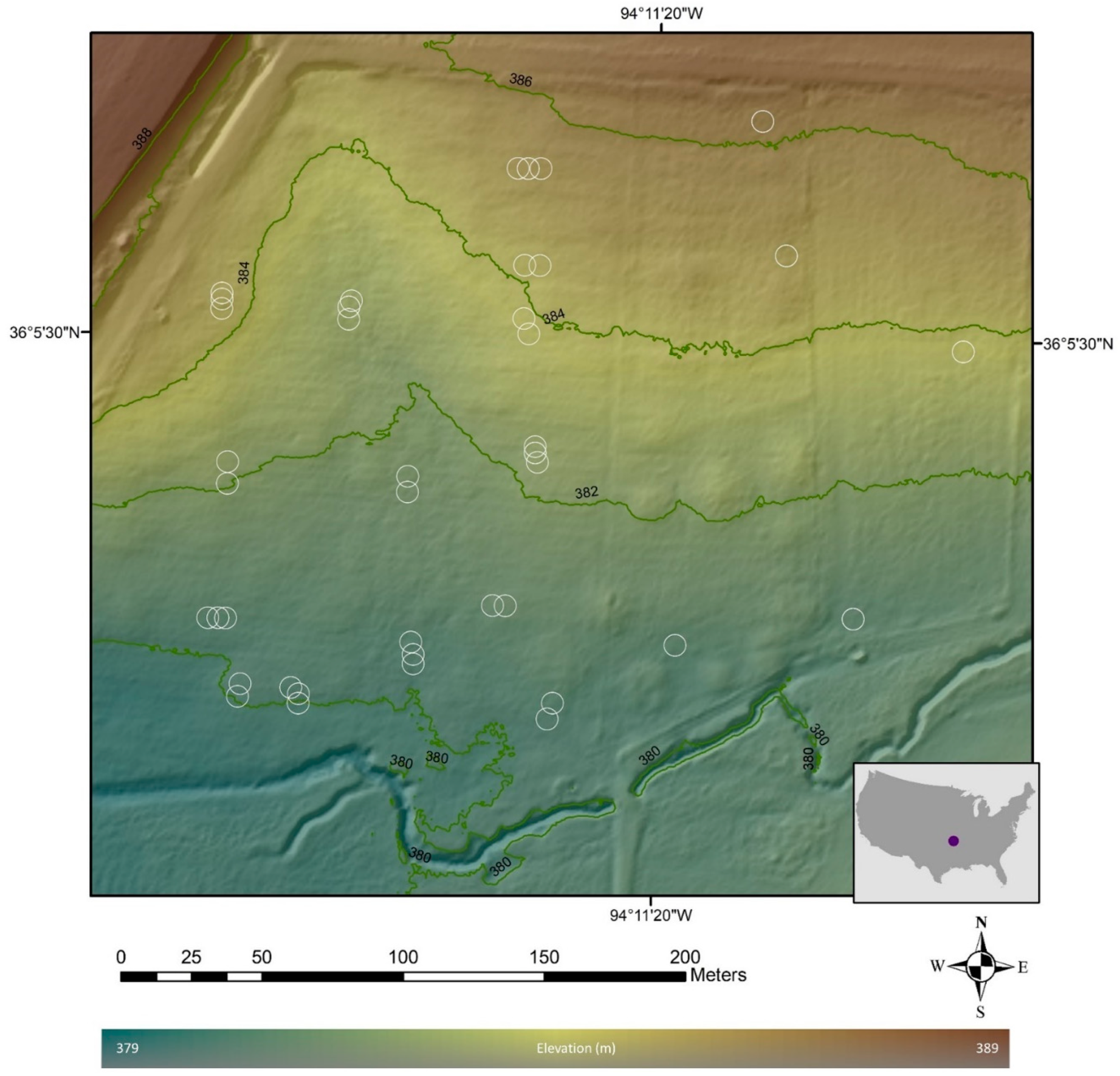
The study site for this investigation was in Fayetteville Arkansas, USA at approximately 36.09 degrees latitude and −94.19 degrees longitude (
Figure 1). The climate is considered humid subtropical in the Köppen-Geiger climate classification system [
49]. The annual total precipitation is around 1200 mm per year and mean annual temperature ranges from 13–15 °C, with a pronounced cold winter and warm humid summer. The bedrock geology is described as Mississippian and Pennsylvanian with depositions ranging from shallow marine to terrestrial and is interpreted to “reflect the interplay of tectonics and eustasy during the Mississippian-Pennsylvanian Periods” [
50]. The study site is 9.9 ha with soils that developed in the Springfield Plateau of the Ozark Highlands [
51].
Elevation for the site ranges from 379 to 387 m. Seventy-three percent of the land area is classed as either “slope” or “footslope” with the Geomorphons landscape classification algorithm and a further 25% classed as “hollow” or “valley” [
52] with a mean slope of 3.3 percent rise, a 1st quartile slope of 2.2 percent, and a 3rd quartile of 4.2 percent. Median slope is 3.1 percent.
The soil at the site is well-developed Ultisol with appreciable amounts of translocated silicate clay and a moderately low degree of base saturation. Both the translocated silicate clay and the fragic properties of some of the soils at the site lead to diminished infiltration rates [
53], thus heightening the potential influence of surface topography on moisture movement through the landscape. The dominant soil series at the site is named Captina, a fine-silty, semiactive, thermic, Typic Fragiudult developed in sloping uplands and old stream terraces in a thin mantle of silty material and underlying colluvium and residuum weathered from limestone, cherty limestone and dolomite or siltstone [
54]. Also included is Pickwick Silt Loam, a fine-silty, mixed, semiactive, thermic, Typic Paleudult developed in silty material and old alluvium; Nixa, a loamy-skeletal, siliceous, active, mesic, Glossic Fragiudult developed in colluvium and loamy residuum; and Johnsburg in the lower elevations of the site, a somewhat poorly drained fine-silty, mixed, active, mesic, Aquic Fragiudult developed in silty material and underlying loamy residuum [
54,
55]. The primary influence resulting in differentiation of the Aquic from the Typic Subgroup at the site is topography, as climate and other soil forming factors are largely uniform at the relevant spatial scale.
We obtained a 1 m resolution digital elevation model made with laser altimetry for the research site from the USGS 3DEP program [
56,
57]. Data were acquired in January 2015 leaf-off conditions using LiDAR Riegl Q-680i sensor mounted on twin engine aircraft; the nominal pulse spacing for acquisition was 0.7 m and the fundamental vertical accuracy was tested at 8 cm [
57]. Light-detection and ranging (LiDAR, or air-borne laser altimetry) bare-earth returns were converted to 1-m elevation rasters through bilinear interpolation [
56]. These DEM data are freely available to the public through the USGS website [
57]. With one exception, we used SAGA GIS (v. 2.3.2 and v. 8.0.1) [
58] for processing DEM data, hydrological correction using minimal modification depression breaching [
59], calculating flow algorithms, calculating slope [
60], and calculating topographic wetness index. The MFDmd flow algorithm (discussed below) was calculated in SimDTA, a software developed for that purpose [
61].
Moisture sensors were installed within treatment blocks of a separate study designed to examine the influence of the performance of pasture grasses between rows of trees and cattle foraging behavior [
31]. Moisture sensors were placed in locations within the grass strips. Sensor locations were chosen by a field soil scientist to represent expected spatial variability of soil moisture within the existing plot structure of the foraging study. Plots were designed to study foraging behavior and forage performance in response to variable fertility. Each plot was outfitted with one soil moisture sensor in a “wet” location, and one in a “dry” location. The sensors were installed at 15 cm and 60–75 cm depths in 42 locations or depths for a single hillslope site of 9.9 ha in April of 2017. In the last year of the study more sensors were installed as the foraging study expanded, increasing the number of sensors to 57 in January of 2021. In a few locations the deep sensors were placed at 45 or 70 cm because restricting layers prevented deeper installation. The temporal resolution of the sensors was one reading every four hours and the number of VWC observations after excluding outages and applying quality control was 274,681 readings for the 5-year period. The TEROS 11 sensors estimate VWC using capacitance/frequency-domain technology at 70-MHz frequency, which minimizes textural and salinity effects; accuracy is reported to be ±0.03 m
3/m
3 with the factory calibration on a typical mineral soil; resolution is 0.001 m
3/m
3 (METER Group, Pullman, WA, USA). No special site-specific calibration was performed [
62]. Readings were logged on a Decagon EM50 data logger (METER Group, Pullman, WA, USA).
Moisture data were interpreted and used in the following way. Any moisture readings with greater than 0.5 m
3/m
3 volumetric moisture from a functional moisture sensor were assumed to represent saturated soil and were imputed with the value 0.5 m
3/m
3. Similarly, any moisture readings less than 0.03 m
3/m
3 from a functional moisture sensor were assumed to represent dry conditions and were imputed to the value 0.03 m
3/m
3. These values were chosen as the upper and lower range for saturated and dry mineral soils in the study landscape based on the reported error of the sensors and the soil water retention curves published by the National Cooperative Soil Survey Laboratory Data database of the United States Department of Agriculture for the soils at the site [
63]. More details of data handling are given in the coverage of statistical methods below.
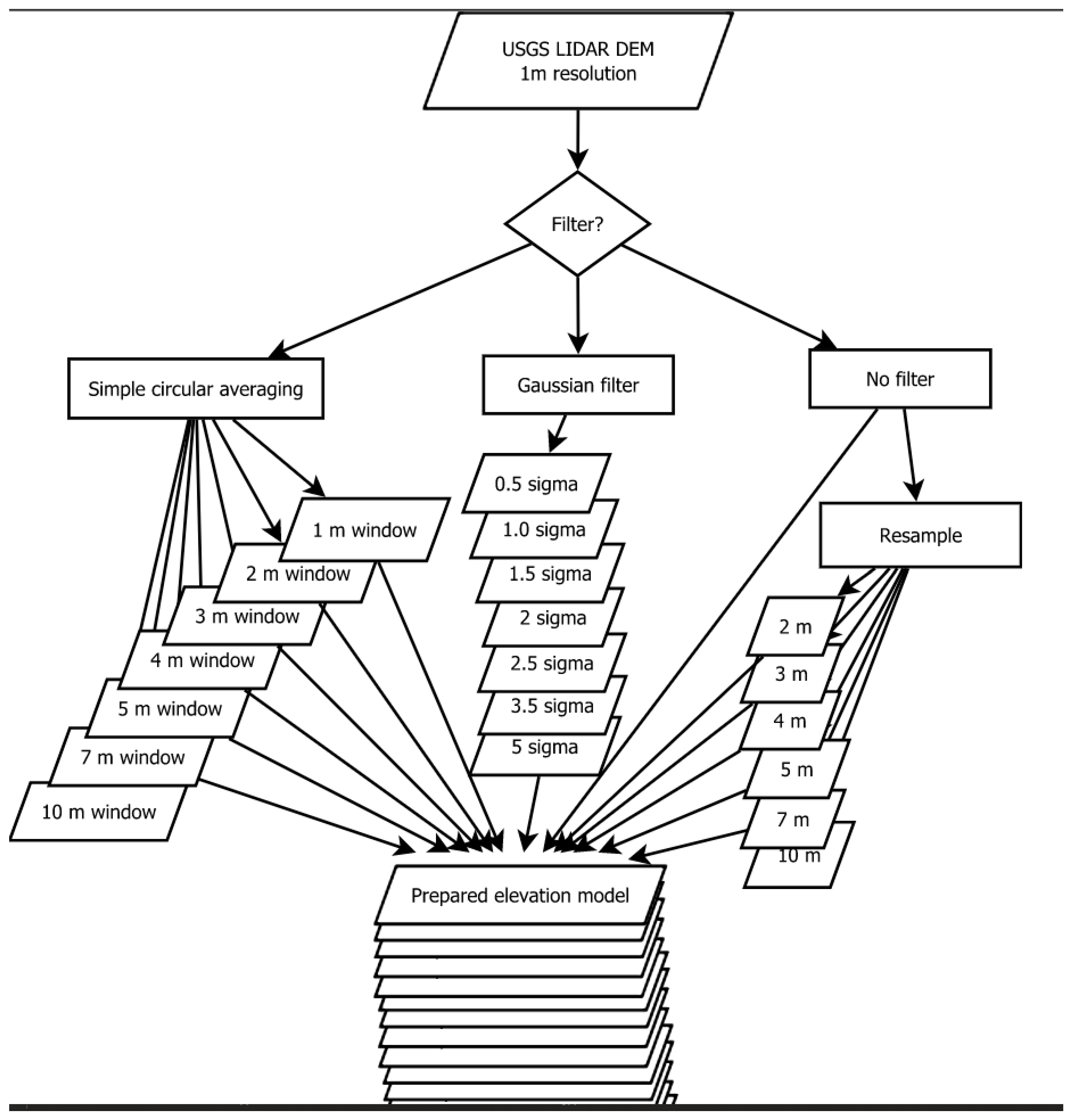
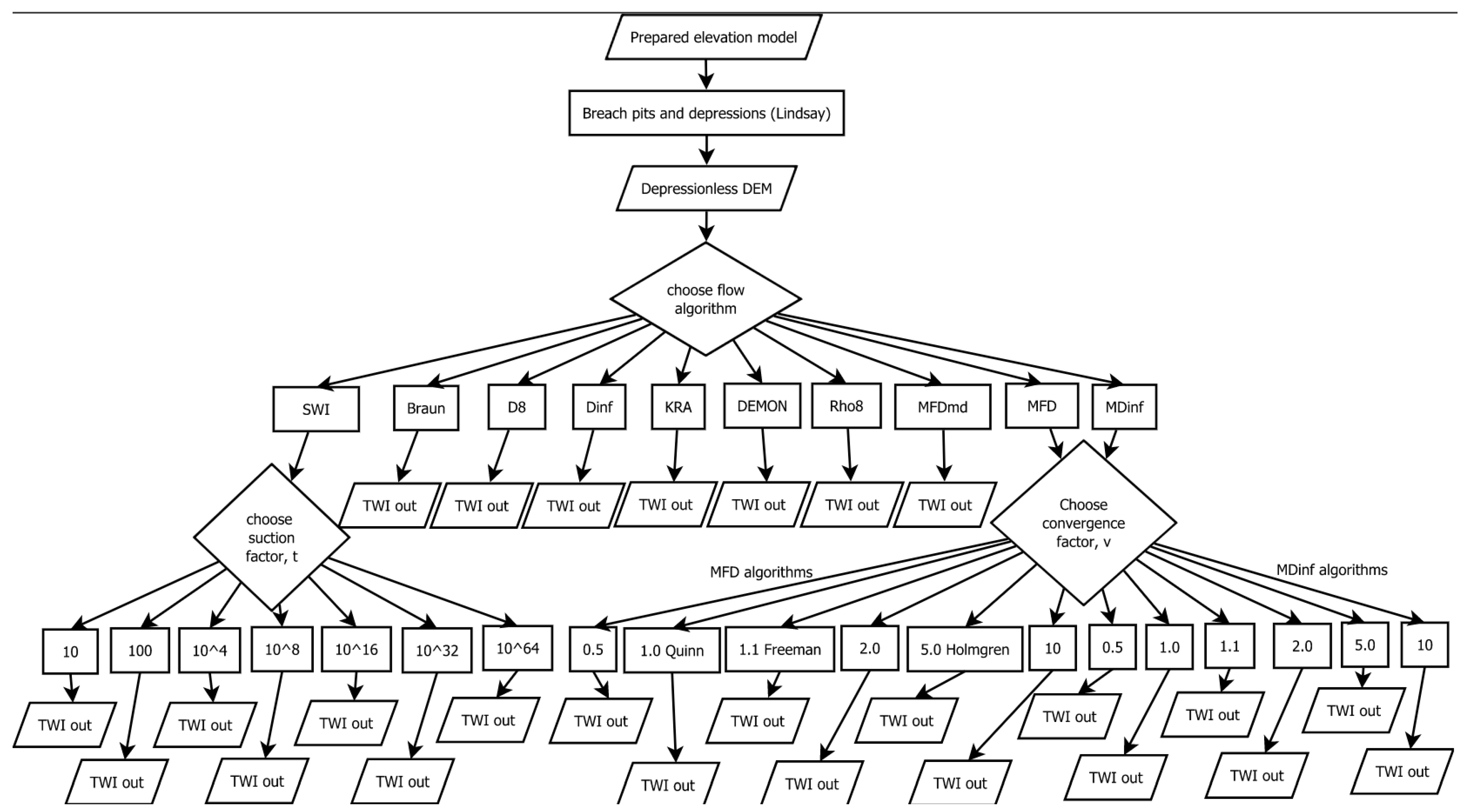
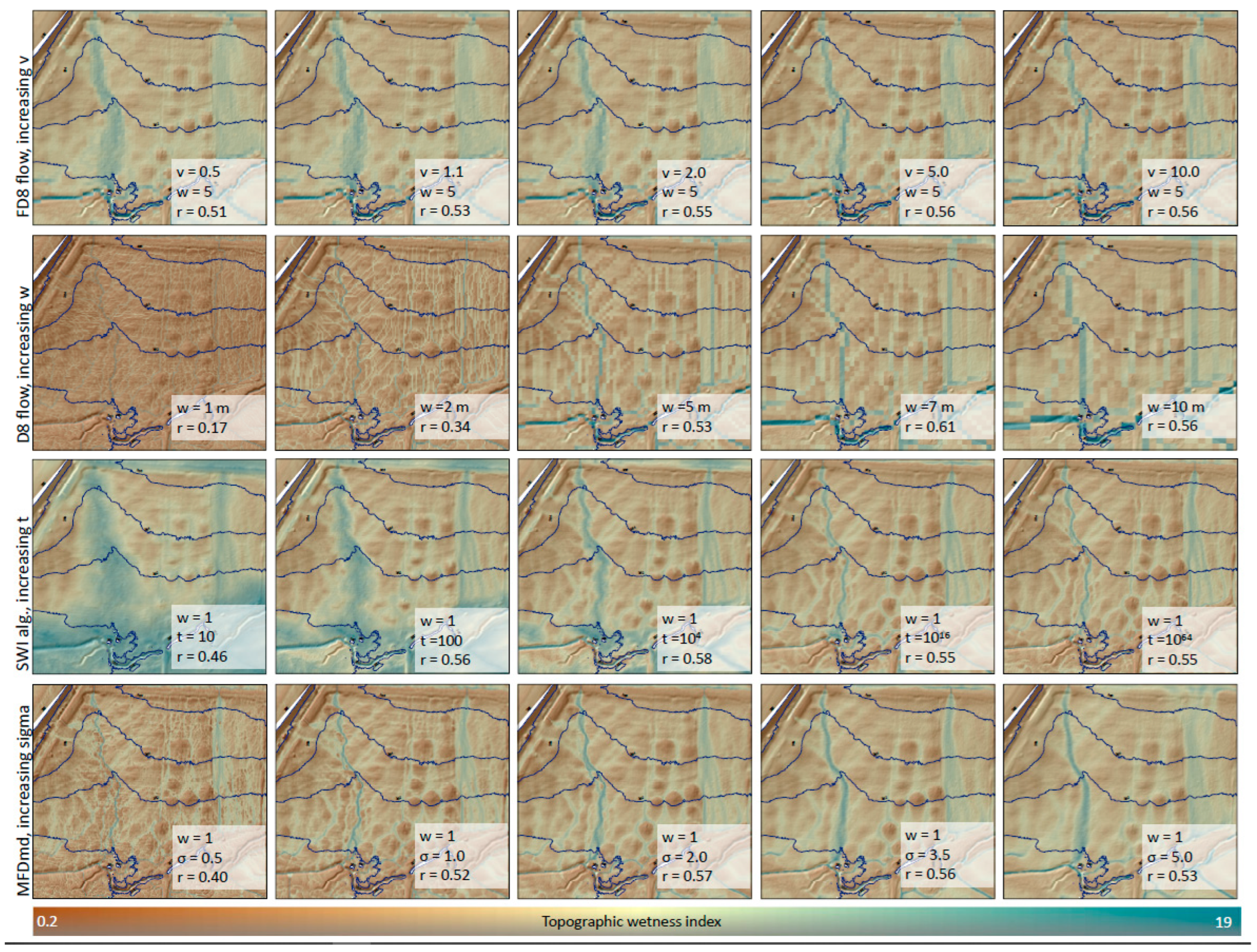
We prepared 21 digital elevation surfaces through filtering and resampling of the source DEM for input into 26 topographic wetness algorithms, deriving a total of 546 topographical wetness index rasters for the site (
Figure 2). The purpose of the generalization of the DEMs through resampling or filtering was to test the degree to which generalization provides control over excessive surface detail. Filtering was undertaken with either a simple circular averaging filter with an averaging kernel, or through a Gaussian filter kernel (
Figure 2). In both cases, the kernel was modified to various settings to test the sensitivity of the TWI to the degree of smoothing. The original unfiltered DEM, and DEMs resampled to larger pixel sizes were also included for comparison. The low-frequency spatial filtering was used to minimize high-frequency noise in the original DEM because “differentiation of a signal increases noise manifestation in a derivative”, and noise in a DEM leads to production of more noisy models of morphometric derivative attributes [
11]. Unfiltered DEMs were resampled to 2, 3, 4, 5, 7, and 10 m using averaging. The elevation value for the 2 m pixel was calculated by averaging the four 1m pixels that fell within its geographic location. The 5 m pixel was assigned an average of the 25 pixels of the original 1 m DEM that fell within its location, and the other resampled DEMs were calculated the same simple way. The 1 m, unfiltered DEM was left unmodified before algorithm preparation.
A common practice when preparing digital elevation models for hydrological terrain analysis is flow path enforcement through the removal of spurious pits and peaks, typically by filling a DEM [
64,
65]. This solves the problem of discontinuous flow as local micro pits are “filled” so that flow within the structure of a landscape is given an outlet point, and flow is not unrealistically disrupted by “disappearing” into pits. Filling pits at the DEM for our research site resulted in excessive generation of flat depression surfaces and was considered unacceptable, as it changed elevations and eliminated real topographic detail for about 66% of the study area. Instead, a DEM depression breaching algorithm was chosen, which successfully eliminated closed depressions with minimal alteration of the elevation model while enforcing continuous flow paths through carving [
59,
64].
Filtered DEMs were processed with averaging filters of either Gaussian or simple circular shape. In the case of the circular filter, the average value of all pixels within a circular moving window of a specified radius was assigned to the central pixel. The moving window was set to 1, 2, 3, 4, 5, 7, and 10 pixels to give output DEMs on a continuum of an increasing degree of smoothing to the initial elevation model. For Gaussian filtering a given value of sigma was chosen to represent the shape of a three-dimensional Gaussian curve. The values of sigma were chosen as 0.5, 1.0, 1.5, 2.0, 2.5, 3.5, and 5.0 pixels to cover approximately the same area as the simple circular filter. The value of the central pixel in the Gaussian filtration was assigned according to the standard Gaussian probability density function.
The 26 algorithm settings chosen to calculate the topographical wetness index and applied to the 21 prepared (original, filtered, or resampled) elevation models for the site differ primarily in their implementation of flow algorithms (
Figure 3). Flow algorithms allow for the calculation of the catchment area or A, the numerator in Equation (1). Catchment area is calculated by tabulating the number of pixels that would contribute runoff flow to the receiving pixel in a scenario in which no water is absorbed in the soil and flow is determined by gravity. Flow algorithms determine the direction of flow from higher elevation pixels to lower elevation pixels [
12,
13]. They are broadly classed as single-direction flow and multiple direction flow algorithms. Multiple-direction flow algorithms can be further subdivided based on whether flow is limited to two or three receiving neighboring pixels. A review of flow algorithms can be found in Wilson [
13], but we will also summarize them here.
Figure 3 illustrates the flow algorithms and the decision points for various algorithm settings tested in this study.
Single-direction flow algorithms model flow from the source pixel to a single receiving pixel typically determined by calculating the direction of steepest descent. These algorithms were developed to aid in the extraction of drainage networks from digital elevation models and not necessarily for depicting variable soil moisture. They are the default option in several GIS software applications, though they perform less well when flow dispersal is an important feature of a landscape, or when ridges, peaks, and saddles are present [
13,
34].
The deterministic single-flow (D8) algorithm routes flow from the central pixel to the lowest of its surrounding 8 grid cells [
14]. It was the first flow algorithm developed and is the simplest and the quickest to calculate. The stochastic single-direction flow algorithm (Rho8) includes a random element into the assignment of flow directions designed to reduce grid bias [
13,
66]. Output from Rho8 is different each time it is run, unless specifying a pseudorandom number generator seed. Aspect-driven kinematic routing (KRA) assigns flow to cardinal directions while specifying flow direction continuously [
67]. KRA calculates contributing area by summing the number of flow paths passing through a grid cell.
In multiple flow direction algorithms flow is dispersed to multiple downslope pixels [
68]. The first of these algorithms are limited in the number of receiving pixels. In the deterministic infinity (Dinf) algorithm flow direction is assigned to each cell by a continuous value from 0 to 2π. The vector describing flow direction determines the proportions of flow that are distributed to two receiving pixels on the two sides of the drainage flow direction vector [
69]. The Braunschweiger multiple flow direction (Braun) algorithm limits flow to three receiving pixels, routing outflow to the cell with orientation nearest to the aspect of the source cell and its two neighboring cells [
38,
70]. The Digital Elevation Model Networks (DEMON) flow routing algorithm involves the use of best-fit planes through the four corners of a pixel and allows flow to two receiving pixels [
71].
Multiple-flow algorithms that direct flow to all eight surrounding pixels include the multiple flow direction (MFD), multiple triangular flow direction (MDinf), multiple flow direction with maximum downslope gradient adjustment (MFDmd), and the SAGA Wetness Index (SWI). The Mass Flux (MF) algorithm (not examined in this paper) divides each grid cell into four quarters and defines a continuous flow direction for each depending on the elevation of the whole pixel and two of its cardinal neighbors; flow from each quarter of the central pixel is then allowed to flow into one or two of its cardinal neighbors [
13].
In the multiple flow algorithms MFD [
68,
72,
73], MDinf [
74], MFDmd [
61], and SWI [
75] the fraction of a pixel’s flow (d) moving to a neighboring cell (NBi) is calculated with:
where L is the draining contour length and v is the flow dispersion exponent [
13,
38,
76]. As the v-value increases more of the fraction of flow proceeds to the steepest slope resulting in a higher degree of flow convergence. Different authors have recommended different values for the constant v-value. The original algorithm also included a different L-value for flow routed to diagonal vs. cardinal directions, but this is not implemented in the SAGA software used in this study and similar studies [
36,
38].
Quinn [
68] used a v-value of 1.0 while Freeman [
72] recommended a v-value of 1.1, and Holmgren [
73], working at elevation sites with steeper relief recommended values between 4 and 6. It has been recommended to use higher values of v in landscapes with steeper slopes and lower values in less sloping landscapes [
76]. Qin et al. [
77] developed the MFDmd algorithm which implements a dynamic v-value based on local slopes for each pixel by calculating v in Equation (2) with the function:
where e is the maximum downslope gradient and min(e, 1) is the minimum of e and 1. The coefficient 8.9 is set so that f(e) will be close to 1.1 in flat areas and as high as 10 in steeply sloping areas. This implementation of the algorithm takes the task of defining the value of v away from the user, possibly leading to more consistent results across landscapes with various magnitudes of slope. Furthermore, it confers the advantage that the user need not define a single v-value in landscapes characterized by both flat and sloping areas together [
77]. The authors of this algorithm indicated that its implementation in the SAGA-GIS software had at least one error and they offered to run the elevation models for our study in their own software program, SimDTA (Qin 2022, personal communication, January 15). This is the only flow algorithm implemented for this study that was not done in SAGA-GIS.
The MDinf triangular multiple-flow direction algorithm directs flow using triangular facets similar to Dinf and behaves similarly in most landforms, but it allows flow to diverge in multiple directions when landforms direct divergent flow, where more than one steepest downslope direction from a cell occurs, such as on divergent hillslopes, ridges, saddles, and summits [
12]. Where flow divergence is allowed, the MFD flow algorithm of Quinn is used, and values of v govern flow divergence partitioning. In the current study, the MDinf algorithm tended to be among the best at matching observed soil moisture. In our results, its output was not highly influenced by the v-values chosen, presumably because v-values are only relevant in areas where flow divergence occurs in the algorithm with divergent downward sloping directions from a given pixel.
The SAGA Wetness Index (SWI) is an implementation of the v = 1.1 multiple direction flow algorithm that iteratively modifies the catchment area based on a function of local slope and the flow accumulation of pixels adjacent to each pixel [
71,
74]. The SWI concept assumes that pixels adjacent to one another will have influence through “suction” or lateral moisture movement due to soil porosity and that this influence increases in flatter terrain. The flow accumulation is thus calculated using the upstream contributing area and the MFD given in Equation (2), but then adjacent pixels were assumed to contribute additional flow accumulation units locally based on the formula:
where SWI is the saga wetness index, SCA
M is a modified specific catchment area,
t is the so-called “suction factor,” a parameter entered by the user, SCA
Max is the maximum stable value for SCA
M obtained through the iterations, and β is slope. The iterative algorithm allows adjacent pixels to contribute flow and continues for as long as the modified specific catchment area is less than the new modified specific catchment area. Increasing slope values and increasing t values both diminish the influence of adjacent pixels, thereby lessening the modification of the original specific catchment area. In the Saga GIS software, the default t value is set to 10 but can be modified by the user. In the original publication introducing the SWI, the equation above is given with a constant value of 15 (where the value
t is placed in the above equation) [
75] (Böhner and Selige, 2004). The formula parsed above was confirmed with the developers of the algorithm (J. Böhner 2021, personal communication, 2 November 2021). Following other authors [
38], we tested the sensitivity of the
t factor for its influence on the correlation between the SWI and observed soil moisture. While some authors [
38] found that higher values of
t led to greater coefficients of determination between the SWI and the observed soil moisture the highest value they chose to examine was
t = 256. We increased our tested values by doubling orders of magnitude from
t = 10 to
t = 10
64. This high value was chosen as the endpoint because the output of SWI rasters began to converge when
t values were set between
t = 10
32 and
t = 10
64.
Statistical Analysis
We used TWI calculated with each of the 546 different outputs from flow algorithms and DEM preparations to predict soil moisture (VWC) at several different temporal resolutions at point locations corresponding to the soil moisture sensors. We used the following time periods and constraints:
Mean VWC for each month (April 2017–December 2021). A moisture-sensor-month combination was only included if the sensor gave readings for at least 10 unique days during that month.
Mean VWC for each year (2017–2021). A sensor-year combination was only included if the sensor gave readings for at least 7 unique months, in each of which there were at least 10 unique days of readings.
Grand mean VWC for the entire measurement period.
Mean VWC by day during three months in the water year representing recharge, saturation, and use periods in the water year, represented in November, April, and September for the years 2017, 2018, 2019, 2020, and 2021.
For every combination of period and algorithm, we generated four sets of predicted values:
We fit a linear regression of VWC on TWI using data from all sensors with valid readings for the given time slice, then used that regression to generate predicted values for all sensors.
We fit a linear regression of VWC on TWI and the depth of the sensor using data with valid readings during the time slice, then used that regression to generate predicted values for all sensors.
We fit a linear regression of VWC on TWI using spatially blocked cross-validation (CV). Each cross-validation had as many folds as there were sensors used to fit the regression. For each CV fold, we omitted all data points from a single sensor (1 to 3 data points depending on how many moisture probes were connected to the logger). The sensors attached to a single logger are spatially adjacent, making this is a conservative approach to address potential spatial autocorrelation in soil moisture unrelated to TWI. Within each fold, we fit the regression to all data except for the value(s) from the held-out sensor, then predicted the value(s) from the held-out sensor. We combined the predicted values from each CV fold, resulting in a vector of predicted values corresponding to all observed values.
We fit another linear regression using spatially blocked CV in the same way as above but included both TWI and depth of the moisture sensor as predictors.
For each of the above four sets of predicted values, we took the Pearson correlation r between observed values and predicted values (combining predictions across all CV folds in the latter two cases) as a metric of prediction performance.
All data processing and model fitting was done using R software, version 4.1.2. Models were fit with the lm() function.
In the more successful iterations of the TWI settings, higher values of TWI correspond to greater degrees of wetting and greater consistency of moistness throughout the measurement period while lower values of TWI correspond to drier areas. Ambient drying and wetting conditions at the site represented continuous levels of establishment and disruption of a steady state of moisture conditions and therefore greater or lesser topographical organization of soil moisture [
41].
3. Results
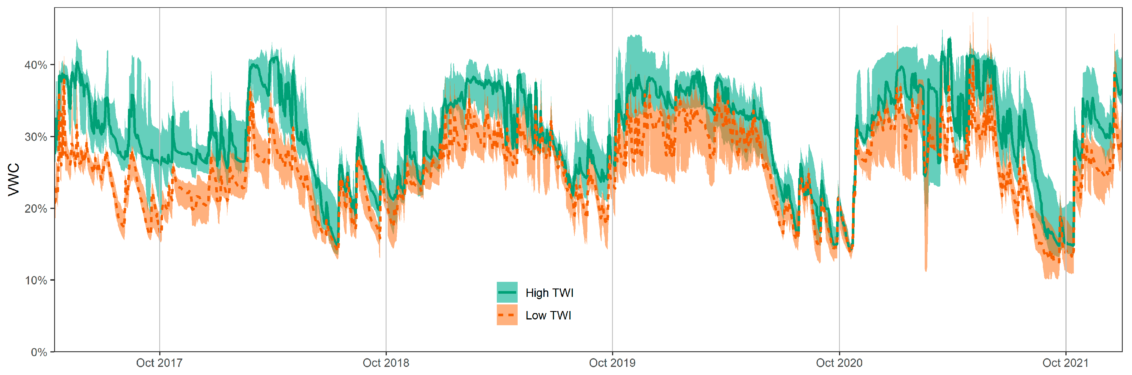
Soil volumetric water content at observation points at the site fluctuated daily and seasonally, with some abrupt influxes corresponding to daily precipitation events followed by more gently sloping episodes of decrease or drying-out (
Figure 4). In most water years, the lowest average values for VWC were found near the end of the growing season in September or October when soil moisture use and evapotranspiration were greatest. Following this, a recharge period from October to January or February led to increases in VWC, reaching saturated conditions before the latest spring frost date and the onset of increased evapotranspiration in May. Moisture sensors at locations with higher TWI values consistently showed higher VWC, but the magnitude of the difference varied with season and apparent rainfall events (
Figure 4).
TWI and soil moisture at the site were positively correlated, with median monthly Pearson correlation coefficients of 0.50 across all algorithms for the models that include a depth component, indicating that TWI has some predictive power for determining areas at the site more prone to retain moisture than other areas.
The most influential single factor for model performance at all time resolutions was DEM generalization. We refer here to filtering and resampling as map generalization. TWI algorithms that were run on DEMs that were generalized through resampling to coarser pixel sizes or through Gaussian or simple circular filtering provided a better fit to measured moisture than non-generalized DEMs, or DEMs taken from the initial LIDAR dataset at 1 m pixel resolution with only the depression breaching algorithm applied before TWI calculation (
Figure 5).
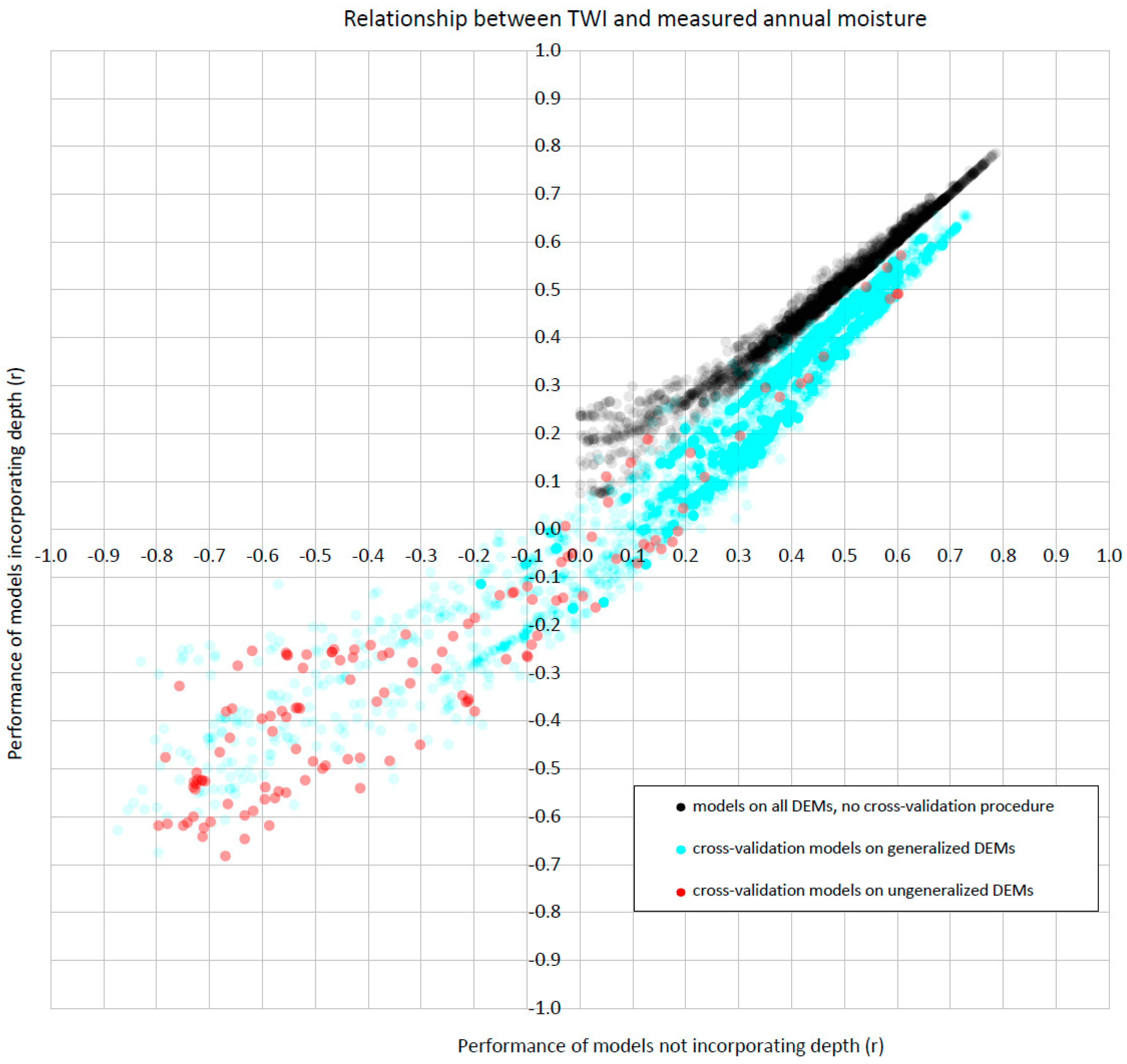
Annual average VWC compared to TWI values extracted for the point locations of the moisture sensors showed wide variation in model performance, with Pearson correlation coefficients ranging from 0 to nearly 0.8 (
Figure 6). In almost all cases, overall model performance improved substantially when the original DEM was resampled to coarser pixel sizes or when it was filtered with a Gaussian or a simple circular smoothing filter to remove or generalize surface detail. Lower correlations occurred disproportionately with iterations of TWI that were applied to DEMs that had not been filtered or resampled. On DEMs that were not generalized, 85% of the cross-validated models had r values less than 0, indicating no reliable performance with respect to spatial prediction of soil moisture at the site. On maps that were generalized, performance improved to 79% of cross-validated models with r values greater than 0, indicating some predictive capability. Model performance also improved when moisture sensor depth was included, though the improvement was most marked when initial performance was poor. The best performing models without depth showed little improvement when depth was included, while the poor performing models, such as those with r values below 0.3 improved much more.
Generalization through increasing the pixel size by resampling resulted in a linear increase in median TWI performance when DEM pixel size was increased from 1 to 7 m and a slight decrease from 7 to 10 m (
Table 1). Generalization through filtering the 1 m DEMs with a simple circular averaging filter also improved model performance with the highest performance reported for the 5 and 7 m radius filter windows, with a slight decline at the 10 m radius. Gaussian filtering showed a similar effect, with the best performance at 3.5 sigma and a small decline at 5.0 sigma.
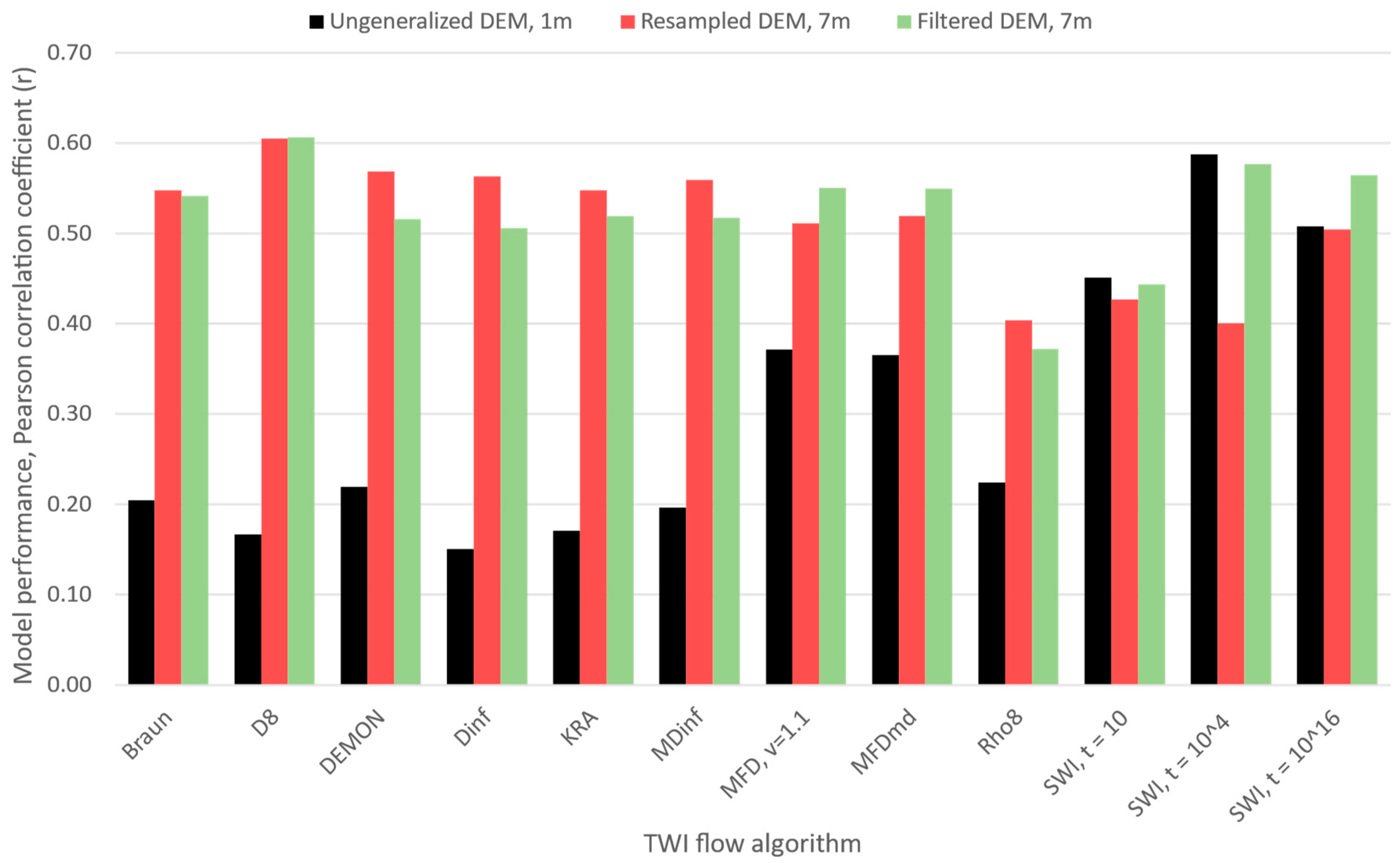
Varying the flow algorithms for calculating catchment area influenced model performance at predicting annual soil moisture to different degrees (
Figure 7). In general, the multiple flow direction algorithms outperformed single-direction algorithms when run on the initial 1 m DEM, unmodified except for hydrologic correction. The best performances of TWI models on the unmodified DEM were from the SAGA Wetness Index with a suction factor in the range of t = 10
4 to t = 10
16. When elevation models were resampled to 7 m, however, single-flow algorithms performed at a similar or sometimes better level. The D8 algorithm applied to a resampled 7 m elevation model gave the best performance for predicting annual soil moisture of all algorithms. Filtering was a better strategy for map generalization when using multiple flow direction algorithms while resampling was better for single-flow direction algorithms.
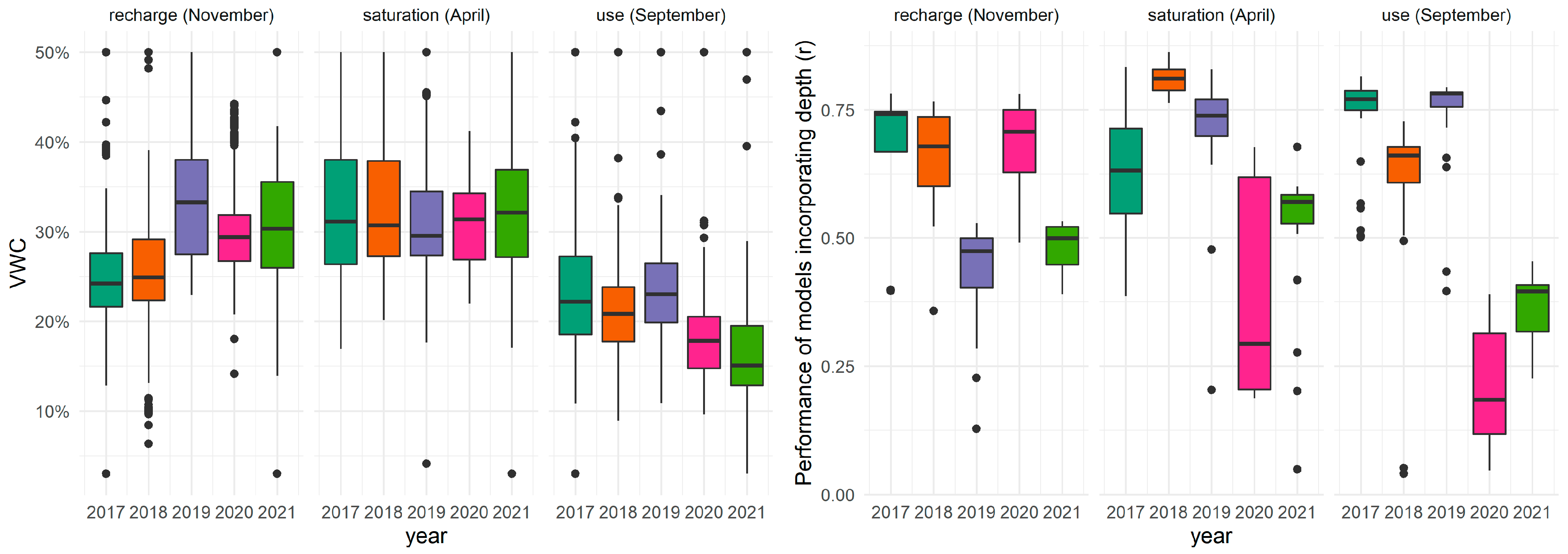
Correlations between VWC and TWI were sensitive to seasonal variation and presumed antecedent moisture conditions relating to spikes in VWC from precipitation events (
Figure 8). Daily VWC during recharge showed good correlation to TWI in November of 2017, 2018, and 2020. In November of 2019 and 2021, however, VWC was relatively high, and correlations were lower than in the other months. During the saturation period when soils are wettest, before the onset of seasonal evapotranspiration in May, correlations between TWI and VWC were high except in the two wettest months with highest median VWC, 2020 and 2021. Presumably, even though moisture conditions were high in the other years, there was enough drying time or time for topographic redistribution of moisture to maintain high correlations with TWI. In 2020 and 2021, however, moisture conditions were at their highest and topographic organization of moisture did not occur as reliably, making correlations between TWI and VWC relatively low. In September, when evapotransporative demand is at its strongest, correlations between TWI and VWC were high. The exception here was again 2020 and 2021, in which very low values of VWC likely led to low correlations between TWI and VWC. In dry conditions, soil texture may govern soil moisture to a greater degree than topography, and the spatial correlation between soil moisture and topography reduces at both the dry and wet end of field conditions [
41].
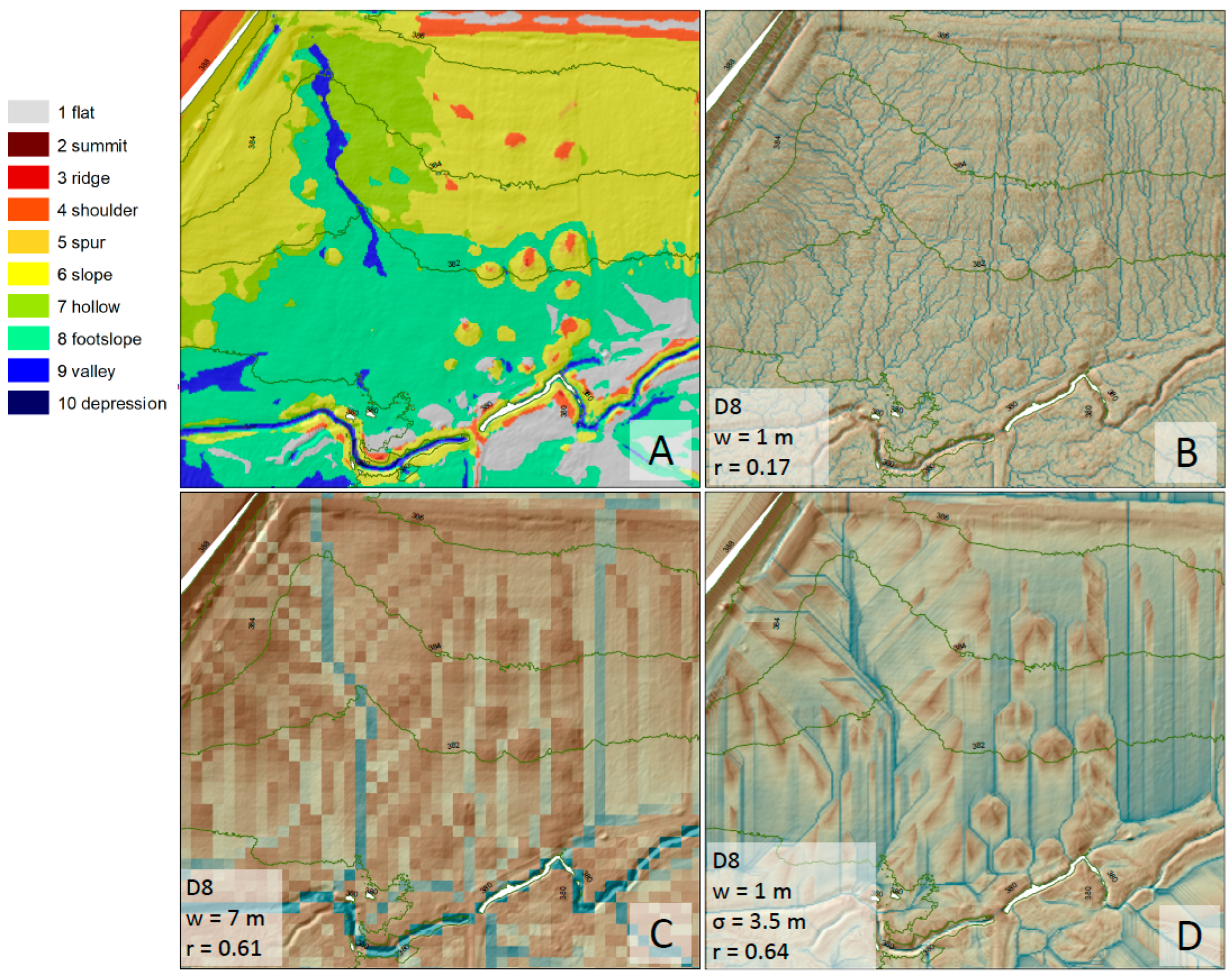
Map generalization improved TWI moisture prediction by allowing flow patterns to coincide with surface moisture as it encounters and responds to landform features (
Figure 9). The site is characterized by side slopes which funnel water toward a primary central valley-shaped drainage area, which directs water further downslope toward a channel at the southern end of the site (
Figure 9A). When the TWI D8 flow algorithm was run on the w = 1 m DEM, the convergent valley zone did not represent unified flow accumulation. Instead, flow converged in multiple very small flow lines pertaining to the noise and roughness of surface topography (
Figure 9B). Many of the flow lines do not converge to a dominant central flow area as would be expected by the landform figure, but flow is instead directed south as relatively independent lines that have little influence on directly adjacent drier areas. Once these flow lines reach the valley area from upper sloping areas, they still do not converge into a single dominant flow zone. As the pixel size (w) is increased through resampling, however, flow lines do converge and become larger in magnitude in valley areas (
Figure 9C). Likewise, when the elevation model is filtered before application of the TWI D8 flow algorithm, flow lines follow the general trend of the shape of the landscape instead of discrete portions directed by surface roughness (
Figure 9D). After generalization, either through resampling or DEM filtration, the grand mean correlation (r) between the TWI with D8 flow increased from 0.17 to 0.61 and 0.64, respectively, for the ~5 years of observation.
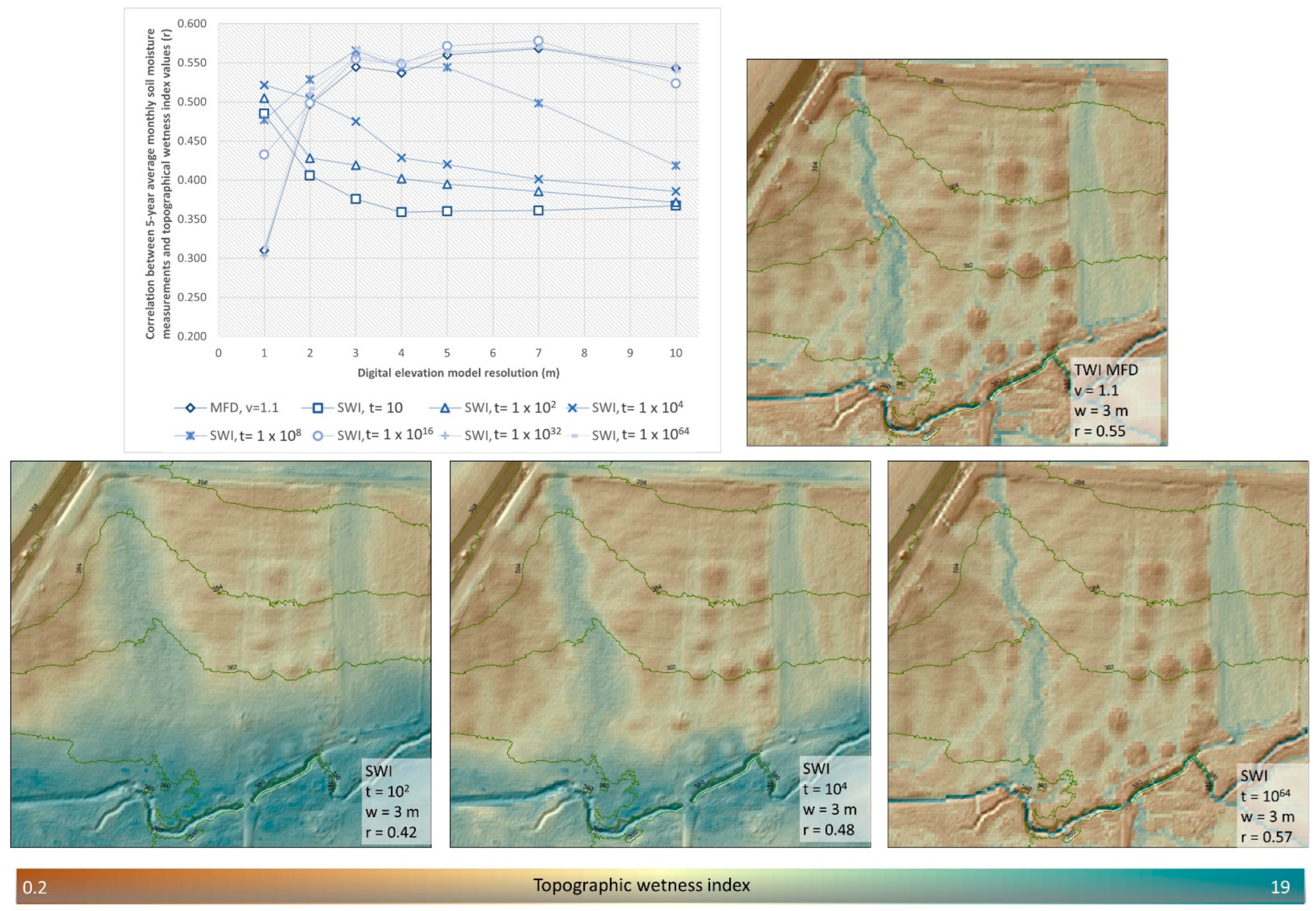
The suction factor (t) of the SAGA Wetness Index influenced the correlation between SWI and grand mean VWC (
Figure 10). At the smallest pixel resolution, w = 1 m, values of
t between 10 and 10
4 gave the best performance; however, when DEM was resampled to larger pixel sizes, the best
t factors were
t = 10
16, 10
32, and 10
64. As
t was increased, its influenced was diminished and the output from SWI more closely resembled output from MFD v = 1.1 algorithm (but r values were slightly higher for SWI with
t values > 10
8 than for TWI MFD v = 1.1). The best performing configurations for SWI were those applied to DEMs that had been either resampled to 3 m to 7 m pixel resolution, or filtered with a Gaussian filter of 2 sigma to 2.5 sigma, or a simple circular smoothing filter of 4 to 5 m. In the cases of filtered DEMs of 1 m resolution, performance improved with increasing suction factor values until
t = 10
4, with a modest decrease thereafter (
Table 2). In the case of resampled DEMs performance increased with increasing suction factor until
t = 10
16 for the DEMs resampled to the 3 to 7 m pixel sizes.
4. Discussion
Factors influencing soil moisture at the field scale are multiple and include precipitation, vegetation variability, solar incidence and shading effects, variation in soil properties such as porosity, soil structure, and soil texture [
3,
78]. To improve our estimates of soil moisture, ancillary and measured data pertaining to these factors should be included in future efforts. Including variables such as soil properties, other terrain variables, and reflectance data would likely have led to improvements of modeled moisture. Soil moisture is rarely as spatially organized as topography, and authors have noted improvement in soil moisture models through use of a weighted combination of indices, rather than a single index [
34,
41]. Authors found improvement of the relationship between soil moisture and terrain indices when including a simple solar radiation simulation and soil property estimates along with the TWI [
34]. The influence of vegetation type on soil moisture at the site is unknown, but we assume the influence of precipitation and topography to be dominant because while vegetation exerts local control on moisture, topography leading to surface and subsurface lateral flow has been characterized as exerting non-local control [
3].
The strength of correlation between TWI and measured soil moisture fluctuates over time. Some authors reported that the degree of correlation between soil moisture and topography lessens at very dry and very wet field conditions [
41]. At very dry times moisture may relate more to soil texture than topography, while at very wet times moisture is likely limited by soil porosity, which often does not vary greatly at the field scale [
41]. Other authors showed that the relationship between TWI and soil moisture varied seasonally, depending on days after rainfall and period of the hydrologic year [
34].
Despite a lack of a high degree of correlation between TWI and spatial patterns of moisture in some studies [
38], TWI remains useful for several reasons. Soil moisture is difficult and expensive to measure, while TWI is easy to calculate when DEM datasets are available. TWI almost always shows some relationship to measured soil moisture, indicating that it has some predictive power, especially when examined at appropriate scale and resolution (
Figure 5). TWI can aid in the sampling design of placing moisture sensors in optimized locations, thereby maximizing the amount of information obtained from the limited resources of moisture monitoring opportunities [
79]. Examining the relationships among the factors of TWI model development such as degree of generalization, choice of flow algorithm, and resolution and scale remains pertinent because TWI continues to be used as a soil moisture proxy. The current study shows that generalization techniques, whether resampling to coarser pixel sizes, or smooth or Gaussian filtering of LIDAR 1m DEMs, significantly improved the relationship between TWI and measured soil moisture at the study site.
The groundwater table is sometimes thought of as a subdued version of surface topography [
48], and a filtered DEM surface can be considered a subdued version of the original surface because rough and angular components are replaced by averages calculated over a spatial window. A resampled DEM, likewise, involves taking a spatial average over a specified distance, thus subduing topographic detail in favor of any underlying topographic trend. Performance of most variations of the TWI was poor at the site unless generalization, either through filtering or resampling, was first applied. This poor performance is explained somewhat by excessive surface detail leading to overly particularized flow patterns that did not match the overall landform elements of the site. Conversely, as filtration and resampling were applied to the DEM, a subdued version of the local topography emerged, allowing for more generalized depiction of surface moisture that better matched the observed data. The sole exception to the poor performance of algorithms on non-generalized DEMs was the application of the SAGA Wetness Index with low values of the
t-factor (greater influence of
t). While it may seem possible to construe this as indication of good performance by SWI, better performance was given by other algorithms after first applying a generalization technique to the DEM, either filtering or resampling. The SWI allows for flow in adjacent pixels to influence each other through a suction factor, thereby providing a generalizing or filtering effect, smoothing out excessive flow particularization much as a smoothing or Gaussian filter when applied to a DEM before application of a TWI. The SWI applied the smoothing iteratively and concurrently with the calculation of SWI, perhaps making initial DEM map generalization less necessary.
The locations and number of moisture sensors at the study site were determined according to the needs of a study design pre-dating the current study [
31]. A larger network of sensors at a greater spatial density would likely have been better for assessing spatial relationships among TWI output and measured moisture. Furthermore, targeting the spatial variability of the site by placing sensors according to stratified random sampling or conditioned Latin hypercube sampling strategy would likely have improved the spatial moisture estimates by better exploring the range and structure of the ancillary (TWI) variable [
79].
One somewhat surprising finding of this study is that the D8 algorithm, which is the most rudimentary flow algorithm used here, performed well when the DEM was generalized through filtering or resampling. D8 is susceptible to grid bias, depicting flow only in 8 cardinal and ordinal directions, and does not allow flow to disperse to multiple pixels, making flow look “unrealistic” and choppy. Nevertheless, when the DEM was appropriately generalized D8 provided a better correlation to observed soil moisture than several other algorithms. Some authors [
42] found that the best performance for flow algorithms occurred when pixel resolutions matched the average flow width of applied moisture. Likewise, we found that the D8 algorithm was among the best performing algorithms when pixel resolution matched the width of the landform valley feature at the center of our site or when the DEM was first filtered using a filtration window that likewise provided an equivalent amount of generalization, resulting in flow convergence that matched the pattern of the landform classification.
The Pearson correlation coefficients demonstrated the presence of relationships between TWI and soil moisture. However, their values and influencing factors point to many uncertainties at multiple scales. The resampling to coarser scales while improving the correlation values potentially increases the discrepancies in scale between measured soil moisture at a point and TWI calculated for a grid cell. Also, the uncertainty of the relationship between measured soil moisture and calculated TWI values at a point and pixel, respectively, is further compounded by the influence of filtering and flow algorithms for predicting soil moisture over an extended area beyond the point measurement and individual pixels.

 ,
, 


