Article

Modeling Herbaceous Biomass for Grazing and Fire Risk Management

by
Edward C. Rhodes
1,*,
Douglas R. Tolleson
2 and
Jay P. Angerer
3
1
Texas A&M AgriLife Research, Texas Water Resources Institute, 1001 Holleman Drive East, College Station, TX 77843, USA
2
Texas A&M AgriLife Research, P.O. Box 918, Sonora, TX 76950, USA
3
USDA-Agricultural Research Service, Fort Keogh Livestock and Range Research Laboratory, 243 Fort Keogh Road, Miles City, MT 59301, USA
*
Author to whom correspondence should be addressed.
Land 2022, 11(10), 1769; https://doi.org/10.3390/land11101769
Submission received: 8 September 2022 / Revised: 4 October 2022 / Accepted: 11 October 2022 / Published: 12 October 2022
(This article belongs to the Special Issue Decision Support Tools for Land Management)

Abstract

:
Both grazing and fine fuels management are dependent on the temporal and spatial distribution of herbaceous biomass production. Rangeland and wildland fire managers can both benefit from knowing when and where there is excessive herbaceous biomass buildup. In this study, we compared modeled herbaceous biomass outputs from the Phytomass Growth Simulator (Phygrow) to observe and predict herbaceous production on desert, juniper, and pine sites on the Coconino National Forest in Arizona. Models were validated with: (a) 2 years of quarterly data, and (b) fire season-only data. The Phygrow model showed strong agreement between observed and predicted values year-round on the desert (r2 = 0.73) and pine sites (r2 = 0.69), and a lower, but positive agreement in the juniper sites (r2 = 0.54). Fire season predictions were strong for all ecosystem types (desert r2 = 0.89; juniper r2 = 0.62; pine r2 = 0.94), suggesting that the Phygrow model is well suited to provide valuable decision support information with which to address both rangeland and fire management objectives.

1. Introduction

The temporal and spatial condition of standing herbaceous biomass is a critical element in the planning and implementation of grazing and fine fuel (<6mm diameter; [1,2]) management and/or mitigation practices on forest lands, rangelands, and other non-forested areas [3]. Fuel beds with a large herbaceous plant component may be more susceptible to fire than those only composed of forest fuels [4,5] and can lower the bulk density of the fuel bed [4,6]. The timing and scope of management practices, as well as the risk of wildfires, can be complicated by the dynamic fluctuations of herbaceous fuels. Moisture content, growth rate, and biomass are rather sensitive to changes in weather, season, herbivory, and anthropogenic influences [7]. The ability to measure and model herbaceous fuel loads in near-real time has the potential to aid land managers in estimating herbaceous fine fuel production on a landscape and management unit level [8]. Field data can be incorporated into decision support tools to plan land restoration practices, fuel reduction treatments such as targeted grazing, mowing, or prescribed burning, and to preemptively assign wildland firefighting assets to areas of concern [9].
The Standard Fire Behavior Fuel Models [10] provide a very thorough classification of varying fuel beds found in forested and non-forested systems of the United States; however, the choice of one model classification over another can be difficult in many areas due to climatic and management variables that affect fuel accumulation. For example, depending on grazing management and weather conditions, a single grassland site could fall into a Low (GR2), Moderate (GR4), or Heavy (GR7) classification within a relatively short window of time. This complicates planning practices and hinders real-time decision making. Growth models that simulate plant biomass accumulation, reduction, and decay are an attractive tool for estimating and mapping fuel biomass. Plant growth models such as the Forest Vegetation Simulator (FVS) [11], and the Fire and Fuels Extension (FFE-FVS) [12] are capable of simulating total surface fuel loads. However, Hummel et al. [13] found that the FFE-FVS model underperformed in estimating fine fuels, and the model does not account for fuel reduction due to herbivory. As the pressure on local, state, and federal agencies to manage and protect land and wildlife resources, private property, and human life continues to escalate, new methods of addressing resource evaluation and management must arise to meet the demand without placing undue burden on personnel [9].
While forestry models may be limited in their ability to model growth and accumulation of herbaceous fuels, many simulation models exist for rangelands, shrublands, and other non-forested areas. These models may be useful for simulating hydrology, soil erosion, plant growth, and combinations thereof [14,15,16,17]. Numerous models have been developed to simulate herbaceous biomass on rangelands, including the Simulation of Production and Utilization of Rangelands (SPUR) model [18,19,20], Great Plains Framework for Agricultural Resource Management (GPFARM-Range) [21,22], Agricultural Land Management Alternatives with Numerical Assessment Criteria (ALMANAC) [23,24], Ecological Dynamics Simulation Model (EDYS) [25], Agricultural Policy/Environmental eXtender (APEX) [26,27,28], G-Range [29,30] and the Phytomass Growth Simulator Model (Phygrow) [31].
The Phygrow model is a hydrologically driven, daily time-step plant growth model [31] that has been used to study grazing management [32], hydrological policy and brush control investment [33,34], forecasting of forage availability [35], and drought early warning systems on arid grazinglands in East Africa [36,37,38,39,40], and Mongolia [41,42]. More recently, it has been evaluated to estimate herbaceous biomass for grazing management and fine fuels mitigation for the Department of Defense, and the US Forest Service (USFS) [9,43]. Through the combination of plant community, soil, weather, and herbivory data, the Phygrow model generates daily estimates of plant (fuel) growth, reduction via herbivory by wildlife or livestock, total live and dead biomass accumulation, and live/dead fuel moisture, as well as forecasting high, mid, and low biomass estimates at 30, 60, and 90 days into the future [31,35].
The goal of this study was to field validate the Phygrow model through quarterly measurements of herbaceous plant biomass across three ecosystem sites in central Arizona. This central Arizona region marks a new application of the Phygrow model in the desert southwest ecoregion, therefore our research is focused on how well the model predicts actual biomass throughout the year; and more specifically, how well it models herbaceous biomass, or fine fuels, during the wildfire season. The results of this study could have positive implications for the dual management of grazing and fire resources on US public lands.

2. Materials and Methods

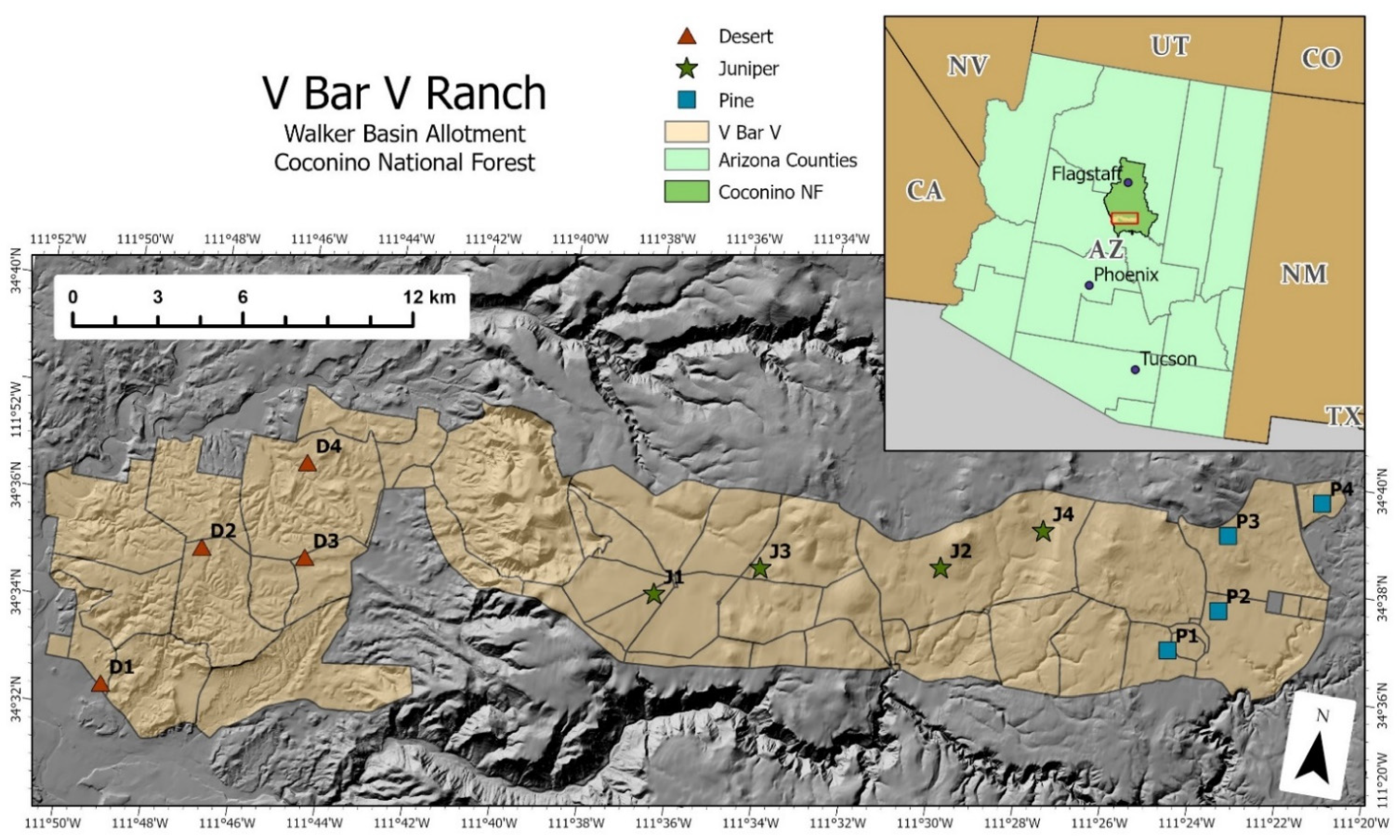
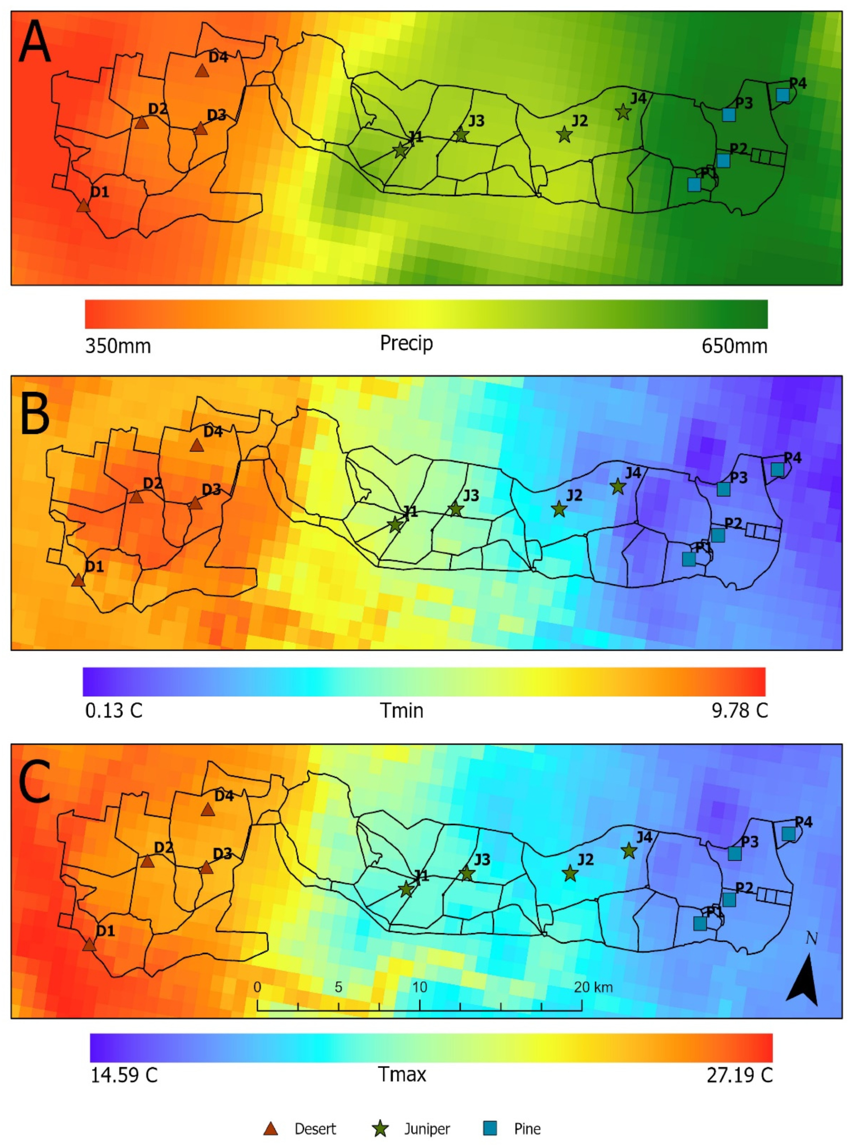
2.1. Site Description

Field data for Phygrow model calibration and validation were collected on the University of Arizona V Bar V Ranch. The 28,732 ha ranch was acquired by the University of Arizona in 1995, and serves as part of the University of Arizona Agricultural Experiment Station [44]. The ranch rests within the Walker Basin grazing allotment on the Coconino National Forest (Figure 1). Plant communities include a collection of grassland, desert shrubland (Prosopis sp., and Acacia sp.), Utah juniper (Juniperus osteosperma [Torr.] Little), alligator juniper (J. deppeana Steud.), and Ponderosa pine (Pinus ponderosa Lawson & C. Lawson) dominated plant communities [45]. Yearly annual precipitation ranges from 350mm to 650mm along a west to east elevational gradient (Figure 2). This area experiences a southwestern US monsoon pattern in which the early summer is typically dry followed by an increase in stochastic convective storms as summer progresses. The transition between these periods, with the co-occurrence of dry fuels and natural ignition is what we labeled as the “fire season”.
For this study, we focused on desert shrub, juniper, and pine dominated ecosystem sites (Figure 1 and Figure 2). Desert sites were the lowest in elevation (960-1200m) and had an overstory dominated by creosote bush (Larrea tridentata [DC.] Coville), mesquite (Prosopis glandulosa Torr.), catclaw acacia (Acacia greggii A. Gray), and barberry (Mahonia haematocarpa [Woot.] Fedde). Dominant perennial grasses on the desert sites included tobosagrass (Pleuraphis mutica Buckley) and low woolygrass (Dasyochloa pulchella [Kunth]). Juniper sites were mid-elevation (1761-1963m), with alligator juniper and Utah Juniper as the dominant woody plants. Blue grama (Bouteloua gracilis [Wild. Ex Kunth] Lag. Ex Griffiths), and sideoats grama (Bouteloua curtipendula [Michx.] Torr.) were the primary warm season perennial grasses, while the cool season western wheatgrass (Pascopyrum smithii [Rydb.] A. Love) was found in the upper end of this zone. Finally, the pine sites were located at the highest elevations (2070-2153m) in ponderosa pine overstories, with pine dropseed (Blepharoneuron tricholepis [Torr.] Nash), Arizona fescue (Festuca arizonica Vasey), blue grama, and Kentucky bluegrass (Poa pratensis L.) dominated understories.

2.2. Data Collection

Field data collected for Phygrow parameterization included plant community and general site attributes. Basic site data included the date of observation, latitude and longitude, transect bearing (azimuth), slope, and aspect. Transect bearings were chosen perpendicular to the slope, and stayed within the same soil association [46]. Attempts were made to visit each site quarterly from Fall 2008, through Summer 2011. Weather conditions at the higher elevation sites intermittently prevented sampling of the juniper and pine sites during the fall and winter months.
We collected plant community data along a 200-footstep pace transect utilizing the USFS Region 3 Common Non-Forested Vegetation Sampling Protocol, or CNVSP [9,47]. The CNVSP protocol is a departure from the standard Phygrow sampling procedure [38,41], and was developed/tested with the USFS to more closely complement the sampling needs of the agency, while still providing data suitable for Phygrow calibration [9] It is a combination of basal cover and frequency measurements in a 40 cm × 40 cm quadrat and a 10 cm × 10 cm nested quadrat (Figure 3). The CNVSP frame is placed along the transect every two footsteps (one pace) for a total of one-hundred placements. Frequency (absence/presence) of all perennial grasses, forbs, and annual grasses are recorded for each quadrat. Woody plant frequency was recorded for those canopies that overlapped a hypothetical vertical extension of the nested quadrat. For Phygrow calibration, we only used the frequency data from the 10 cm × 10 cm quadrat to prevent oversampling of the plant community within the model [9]. Three basal cover pins are located at the 1, 6, and 11 o’clock positions of the outer quadrat (Figure 3) that are used to estimate basal ground cover of rock, surface fuel (ground litter) and perennial grasses. Cover was observed and tallied at the tip of each of the three pins. If the pin contacted the base of a plant, then a plant species hit was recorded. If no plant was in contact with the pin, the ground cover at the tip of the pin was recorded as bare ground, rock, or surface fuel (1-h, 10-h, 100-h, 1000 h).
To calibrate and validate biomass predictions in the Phygrow model, we also collected total standing herbaceous biomass. This required the harvest of all standing live and dead herbaceous material from every tenth lay of the 40 cm × 40 cm (0.16m2) quadrat, drying for 48 h at 70 °C, weighing, and converting into kg ha−1.

2.3. Phygrow Model

Phygrow is a hydrologically driven model that estimates daily plant growth based upon the proportion of each species in the plant community and available soil moisture [31,48]. Water availability is based upon the interaction of soil, climate, vegetative growth, and herbivory [31]. Water storage potential is based upon total soil depth, thickness of each soil horizon, percent rock, saturated hydraulic conductivity, bulk density, infiltration rate, and total water holding capacity. Basic soil characteristics were retrieved from the United States Department of Agriculture (USDA) Natural Resources Conservation Service (NRCS) State Soil Survey Geographic (SSURGO) Database [46], while hydraulic conductivity and water holding capacity estimates were calculated using the Map Unit User File (MUUF) tool [49]. Precipitation was retrieved from the US National Weather Service (NWS) 4km NEXRAD precipitation product [50,51].
Plant communities are parameterized within the Phygrow model using the frequency and point count data collected from the CNVSP protocol. Plant community composition characteristics in Phygrow include basal cover (perennial grasses, rock, litter, and bare ground), frequency (perennial/annual grasses and forbs, woody, and succulent plants), and initial biomass (an estimate used to initiate the model runs) [31]. Each plant species is parameterized with up to 27 attributes, including: minimum and maximum growth temperature, dry matter to radiation ratio, leaf area index, leaf/wood turnover and decomposition rate, and rooting depth [9,31,48]. Baseline values for plant parameters were determined via literature review, local expert knowledge, and from the Food and Agriculture Organization’s ECOCROP database [52].
Herbivory data is entered into Phygrow using stocking rate information (animal units/ha) and dates of movement into and out of the site. Diet selection preferences for each species of herbivore are input and each plant species is marked with a grazing preference during phenological phases (increasing, peak, and declining growth) [31], which is used to drive the daily reduction of forage by herbivory. Plant species or functional group preferences by the grazer are defined as preferred, desirable, undesirable, and non-consumed. For preferred forages, the grazer will eat more of this plant than is found in the plant community on a relative weight basis. Undesirable forages are those that the grazer eats less than what is found in the plant community on a relative weight basis. Desirable forages are grazed at a proportion to that found in the plant community and non-consumed represents plant species that the grazer does not eat or that would be above the browse height of the grazer [31,53].
Given that the central Arizona region was a new area where Phygrow had not been used previously, the model required calibration and verification since new plant species and soils were being evaluated in the model. Calibration of biophysical models generally involves adjustments of a select set of model parameters within the reasonable ranges of these parameters so that model outputs are consistent with observation data and validation is an evaluation of the model outputs against additional and or independently observed data [54]. Vegetation cover and frequency from the summer of 2009 was used to initially parameterize the model to represent peak growth and species richness. Biomass data from the first year of sampling (Fall 2008- Summer 2009) were used for comparisons with model outputs to fine tune growth parameters to ensure proper calibration of the model. The remainder of the biomass samples (Fall 2009-Summer 2011) were used to validate the model (Table 1).

2.4. Statistics

To test the predictive strength of the Phygrow model, we fitted a linear regression of the observed and predicted means in each ecosystem type (desert, juniper, pine). Since r2 is sensitive to outliers and variability in magnitude [55,56,57], we also used index of agreement and root mean square difference to describe model goodness of fit [9,48]. The index of agreement (d) is a measure of the seeming tightness between observed and simulated values [55,56]. In essence, it is a test of the level to which a simulation is error free, where:
d = 1.0 i = 1 n O i P i 2 i = 1 n P i O ¯ + O i O ¯ 2
Here, O is the ith observed value, P is the ith predicted value, and n is the number of observations [55]. The index of agreement ranges from 0 to 1, with increasing agreement between observed and simulated results occurring at higher values of d.
Root mean square difference (RMSD) evaluates model performance by illustrating the average magnitude of the difference between observed and simulated yield (kg ha−1). RMSD possesses more sensitivity to extreme outliers and is often used as a complement to linear regression [55,56,58]. RMSD is computed as:
R M S D = i = 1 n O i P i 2 n
where O is the ith observed value, P is the ith predicted value, and n is the number of observations [55].
Finally, to evaluate the Phygrow model for different objectives such as grazing and wildfire management, the validation dataset was analyzed in whole (Fall 2009-Summer 2011), and by fire season (Summers of 2010 and 2011). Based upon an analysis of the Monitoring Trends in Burn Severity (MTBS) dataset, we observed that 77.5% of the mapped wildfires occurring on the Coconino National Forest from 1989–2012 were in the months of June, July and August [59]. By evaluating the validation dataset in this dual manner, we can test for model viability for estimating year-round biomass for grazing management and for fuel loading during the summer fire season.

3. Results

Phygrow model calibration and validation results are presented in Table 2, and Supplementary Figure S1. Model calibrations were quite high for combined (r2 > 0.97), and each ecosystem type (r2 > 0.8). Year-round model validation showed a strong relationship in desert and pine communities (r2 = 0.73, and 0.69), while the strength of agreement between observed and predicted values in the juniper validation was lower (r2 = 0.54). RMSD (kg ha−1) was rather uniform throughout, except for the juniper and pine calibrations which were higher and lower, respectively. The index of agreement was high (>0.84) for all year-round calibrations and validations. Overall, the juniper communities had comparatively lower r2 and d values than either the desert or pine sites. There was a single outlier in the juniper site dataset from October 2010, that when removed, increased the r2 to 0.61 and d to 0.98. Removal of two outliers from the pine validation increased the r2 to 0.86, and d to 0.96. Values with and without outliers are both presented in Table 2.
Validation metrics for the fire season were higher than the year-round data across all ecosystem types (Table 2). Linear regression values were very high for the desert (r2 = 0.89) and pine (r2 = 0.94) communities. The juniper community was again the lowest with an r2= 0.62, though this was still higher than the year-round validation. RMSD was similar for all ecosystem types, and d was very high as well.

4. Discussion

The Phygrow model was able to sufficiently model herbaceous biomass both year-round and during the fire season. As this was the first broad-scale application for the Phygrow model in the US desert southwest, this supports the use of Phygrow as a dynamic fuel model in this diverse ecoregion. Higher model agreement during the fire season may be attributable to the fact that the vegetation data used for plant community parameterization was collected during the summer, and thus better reflects this growth period. Not being able to access all sites during the fall and winter months may have been partially responsible for the lower regression coefficients for the juniper and pine sites, though the juniper sites had lower agreement during the fire season as well. Herbivory was more dynamic in the juniper sites due to their position within the elevational-based grazing system employed, wildlife distributions in this transitional habitat type, as well as orographically influenced distribution of precipitation [60,61].
Although simulation modeling of rangeland aboveground biomass for rangelands in Arizona is lacking, comparison of Phygrow model performance in Arizona is similar to or better than simulation models used in other rangeland systems. For example, Zilverberg et al. [26] reported r2 values of 0.73 and 0.79, along with index of agreement (d) values of 0.69 and 0.84 for calibration and validation of APEX model simulations against field herbaceous biomass measurements for Kansas shortgrass prairie rangeland. For APEX simulations on Colorado shortgrass prairie rangelands, Cheng et al. [28], had relatively low r2 values (0.26 to 0.32) and moderately high d values (0.69) when comparing total aboveground biomass collected under two different grazing systems. Using the GPFARM model at the same Colorado location, Andales et al. [21], reported d values that ranged from 0.35 to 0.9 for calibration and 0.67 to 0.82 for validation of simulations for different functional groups of rangeland plants with warm season perennials performing better than other functional groups. The performance statistics reported for these 3 studies indicate that the Phygrow simulation model performed well in comparison with other rangeland simulation models.
Year-round modelling gives grazing allotment managers the ability to see current field conditions, as well as potential future conditions, allowing them to plan stocking rate decisions such as pasture rotations, and buying or selling of livestock. The sporadic, and spotty thunderstorm events prevalent in the central Arizona monsoon can create a mosaic of varying levels of biomass production, which can be updated in near-real time with Phygrow. Model outputs in Phygrow are both spatially and temporally explicit and can be used to interpolate biomass/fuel loads into non-sampled areas with similar soils, aspect, elevation, and precipitation, making it useful for grazing and wildfire risk management.
Biomass outputs from the Phygrow model can be used directly to inform decision-making, or may be incorporated into other models and decision support tools such as BEHAVE [62,63], FARSITE [64], the Burning Risk Advisory Support System (BRASS) [65,66], and the livestock early warning system (LEWS) [37] (https://swcarbon.tamu.edu/glews/, accessed on 4 October 2022). For models like BEHAVE and FARSITE, fine fuel outputs from Phygrow could be linked to dynamic fuel maps that can be used to model rate of spread and fire movement, thus providing fire managers with the ability to evaluate fire management options prior to a wild or prescribed fire. Knowledge of fine fuel loads as they relate to available biomass for grazing can provide resource managers and livestock producers with information on the potential impacts that a loss of forage would create should the forage be lost to wildfire which could trigger strategies for fuel break development [67], hay storage, and procurement of forage loss insurance [42].
One potential drawback to using the Phygrow system is that it requires a substantial amount of field data to calibrate and validate the model. Since plant community data for an individual site in Phygrow is a snapshot in time, any substantial changes in vegetation structure will require additional field data and calibration. However, federal agencies on US publicly owned lands routinely conduct field vegetation monitoring for environmental assessment, appraisal of grazing permits, evaluation of restoration projects, and for scientific research. Routine monitoring data may be used to expand Phygrow calibrations to new areas, or to field validate interpolated areas. Repurposing data to model herbaceous biomass provides a value-added product that can benefit the agencies’ grazing, environmental, and wild/prescribed fire planning missions. This added use of data may lead to further collaboration between specialties within agencies, fostering greater synergy of shared visions of land management. Since herbivory is an integral part of Phygrow, prescribed grazing could be modeled as a fuel reduction tool that serves both rangeland and fire management objectives [67,68]. The ability to explicitly model changes in grazing management provides advantages over remote sensing-based approaches for fine fuel monitoring [69,70] in that different grazing managements scenarios could be modeled to evaluate fine-fuel outcomes, therefore aiding in developing adaptive strategies.
Understanding the current and forecasted state of herbaceous field conditions can be very beneficial to making informed land management decisions [40,71]. Herbaceous biomass production has very important implications from both a grazing and a fine fuels perspective [72,73]. Using data across disciplines such as rangeland and wildlife management, grazing permittees, and fire ecology to meet shared goals of proper land management can help lower the overall burden on agencies through mutual collaborations [74]. Moving forward, we recommend that cross-disciplinary approaches that adapt shared collection and analysis of data and objectives to lessen the isolation that often exists between land management specialties.

Supplementary Materials

The following supporting information can be downloaded at: https://www.mdpi.com/article/10.3390/land11101769/s1, Figure S1: Scatterplots and regression fit lines for Calibration, Validation, and Fire Season for Desert, Juniper, Pine, and Combined data.

Author Contributions

Conceptualization, D.R.T. and E.C.R.; field methodology, D.R.T. and E.C.R.; model methodology, J.P.A. and E.C.R.; data collection, D.R.T. and E.C.R.; validation, E.C.R. and J.P.A.; formal analysis, E.C.R.; investigation, E.C.R., D.R.T. and J.P.A.; resources, D.R.T. and J.P.A.; data curation, E.C.R.; writing—original draft preparation, E.C.R.; writing—review and editing, E.C.R., D.R.T. and J.P.A.; visualization, E.C.R.; supervision, J.P.A. and D.R.T.; project administration, D.R.T.; funding acquisition, D.R.T. All authors have read and agreed to the published version of the manuscript.

Funding

This research was funded in part by the United States Department of Agriculture Forest Service, Region 3, Contract Number 08-CR-11031600113.

Institutional Review Board Statement

Not applicable.

Informed Consent Statement

Not applicable.

Data Availability Statement

Not applicable.

Acknowledgments

The authors wish to thank John Kava and the staff of the University of Arizona V Bar V Research Ranch, along with Tim Brown, Katy Gottwald, Krystal Lair, and Josh Halpin for their assistance in field data collection, and to the two anonymous reviewers for donating their time and expertise on this manuscript.

Conflicts of Interest

The authors declare no conflict of interest. The funders had no role in the design of the study; in the collection, analyses, or interpretation of data; in the writing of the manuscript; or in the decision to publish the results.

References

  1. Pyne, S.; Andrews, P.; Laven, R. Introduction to Wildland Fire, 2nd ed.; John Wiley and Sons, Inc.: New York, NY, USA, 1996. [Google Scholar]
  2. Fosberg, M.A. Drying rates of heartwood below fiber saturation. For. Sci. 1970, 16, 57–63. [Google Scholar]
  3. Simard, A.; Main, W. Comparing methods of predicting jack pine slash moisture. Can. J. For. Res. 1982, 12, 793–802. [Google Scholar] [CrossRef]
  4. Miller, C.; Urban, D.L. Connectivity of forest fuels and surface fire regimes. Landsc. Ecol. 2000, 15, 145–154. [Google Scholar] [CrossRef]
  5. Smith, J.T.; Allred, B.W.; Boyd, C.S.; Davies, K.W.; Jones, M.O.; Kleinhesselink, A.R.; Maestas, J.D.; Naugle, D.E. Where there’s smoke, there’s fuel: Dynamic vegetation data improve predictions of wildfire hazard in the great basin. Rangel. Ecol. Manag. 2022. [Google Scholar] [CrossRef]
  6. Brown, J.K. Bulk densities of nonuniform surface fuels and their application to fire modeling. For. Sci. 1981, 27, 667–683. [Google Scholar] [CrossRef] [PubMed]
  7. Dale, V.H.; Joyce, L.A.; McNulty, S.; Neilson, R.P.; Ayres, M.P.; Flannigan, M.D.; Hanson, P.J.; Irland, L.C.; Lugo, A.E.; Peterson, C.J. Climate change and forest disturbances: Climate change can affect forests by altering the frequency, intensity, duration, and timing of fire, drought, introduced species, insect and pathogen outbreaks, hurricanes, windstorms, ice storms, or landslides. BioScience 2001, 51, 723–734. [Google Scholar] [CrossRef] [Green Version]
  8. Li, Z.; Angerer, J.P.; Jaime, X.; Yang, C.; Wu, X.B. Estimating rangeland fine fuel biomass in Western Texas using high-resolution aerial imagery and machine learning. Remote Sens. 2022, 14, 4360. [Google Scholar] [CrossRef]
  9. Rhodes, E.C.; Tolleson, D.R.; Angerer, J.P.; Kava, J.A.; Dyess, J.; Nicolet, T. A comparison of rangeland monitoring techniques for modeling herbaceous fuels and forage in central Arizona, USA. Fire Ecol. 2014, 10, 76–91. [Google Scholar] [CrossRef]
  10. Scott, J.H.; Burgan, R.E. Standard Fire Behavior Fuel Models: A Comprehensive Set for Use with Rothermel’s Surface Fire Spread Model; US Department of Agriculture, Forest Service, Rocky Mountain Research Station: Fort Collins, CO, USA, 2005.
  11. Dixon, G.E. Essential FVS: A User’s Guide to the Forest Vegetation Simulator; US Department of Agriculture, Forest Service, Forest Management Service Center: Fort Collins, CO, USA, 2002.
  12. Rebain, S. The Fire and Fuels Extension to the Forest Vegetation Simulator: Updated Model Documentation; US Department of Agriculture, Forest Service, Forest Service Management Service Center: Fort Collins, CO, USA, 2010.
  13. Hummel, S.; Kennedy, M.; Steel, E.A. Assessing forest vegetation and fire simulation model performance after the Cold Springs wildfire, Washington USA. For. Ecol. Manag. 2013, 287, 40–52. [Google Scholar] [CrossRef]
  14. Bouraoui, F.; Wolfe, M.L. Application of hydrologic models to rangelands. J. Hydrol. 1990, 121, 173–191. [Google Scholar] [CrossRef]
  15. Krueger, E.S.; Ochsner, T.E.; Levi, M.R.; Basara, J.B.; Snitker, G.J.; Wyatt, B.M. Grassland productivity estimates informed by soil moisture measurements: Statistical and mechanistic approaches. Agron. J. 2021, 113, 3498–3517. [Google Scholar] [CrossRef]
  16. Rao, L.E.; Matchett, J.R.; Brooks, M.L.; Johnson, R.F.; Minnich, R.A.; Allen, E.B. Relationships between annual plant productivity, nitrogen deposition and fire size in low-elevation California desert scrub. Int. J. Wildland Fire 2014, 24, 48–58. [Google Scholar] [CrossRef] [Green Version]
  17. Ma, L.; Derner, J.D.; Harmel, R.D.; Tatarko, J.; Moore, A.D.; Rotz, C.A.; Augustine, D.J.; Boone, R.B.; Coughenour, M.B.; Beukes, P.C.; et al. Chapter three—Application of grazing land models in ecosystem management: Current status and next frontiers. In Advances in Agronomy; Sparks, D.L., Ed.; Academic Press: Cambridge, MA, USA, 2019; Volume 158, pp. 173–215. [Google Scholar]
  18. Wight, J.; Skiles, J. SPUR: Simulation of production and utilization of rangelands. In Documentation and User Guide. ARS 63; US Department of Agriculture, ARS: Washington, DC, USA, 1987. [Google Scholar]
  19. Carlson, D.; Thurow, T. Comprehensive evaluation of the improved SPUR model (SPUR-91). Ecol. Model. 1996, 85, 229–240. [Google Scholar] [CrossRef]
  20. Bateki, C.A.; Cadisch, G.; Dickhoefer, U. Modelling sustainable intensification of grassland-based ruminant production systems: A review. Glob. Food Secur. 2019, 23, 85–92. [Google Scholar] [CrossRef]
  21. Andales, A.A.; Derner, J.D.; Bartling, P.N.S.; Ahuja, L.R.; Dunn, G.H.; Hart, R.H.; Hanson, J.D. Evaluation of GPFARM for simulation of forage production and cow–calf weights. Rangel. Ecol. Manag. 2005, 58, 247–255. [Google Scholar] [CrossRef]
  22. Chen, S.; Qi, Z. Parameterizing GPFARM-range model to simulate climate change impacts on hydrologic cycle in a subsurface drained pastureland. J. Soil Water Conserv. 2016, 71, 404–413. [Google Scholar] [CrossRef]
  23. Kiniry, J.; Sanchez, H.; Greenwade, J.; Seidensticker, E.; Bell, J.; Pringle, F.; Peacock, G.; Rives, J. Simulating grass productivity on diverse range sites in Texas. J. Soil Water Conserv. 2002, 57, 144–150. [Google Scholar]
  24. Kiniry, J.R.; Muscha, J.M.; Petersen, M.K.; Kilian, R.W.; Metz, L.J. Short duration, perennial grasses in low rainfall sites in Montana: Deriving growth parameters and simulating with a process-based model. J. Exp. Agric. Int. 2017, 15, 1–13. [Google Scholar] [CrossRef] [Green Version]
  25. Childress, W.; Coldren, C.L.; McLendon, T. Applying a complex, general ecosystem model (EDYS) in large-scale land management. Ecol. Model. 2002, 153, 97–108. [Google Scholar] [CrossRef]
  26. Zilverberg, C.J.; Williams, J.; Jones, C.; Harmoney, K.; Angerer, J.; Metz, L.J.; Fox, W. Process-based simulation of prairie growth. Ecol. Model. 2017, 351, 24–35. [Google Scholar] [CrossRef] [Green Version]
  27. Zilverberg, C.J.; Angerer, J.; Williams, J.; Metz, L.J.; Harmoney, K. Sensitivity of diet choices and environ-mental outcomes to a selective grazing algorithm. Ecol. Model. 2018, 390, 10–22. [Google Scholar] [CrossRef]
  28. Cheng, G.; Harmel, R.D.; Ma, L.; Derner, J.D.; Augustine, D.J.; Bartling, P.N.S.; Fang, Q.X.; Williams, J.R.; Zilverberg, C.J.; Boone, R.B.; et al. Evaluation of APEX modifications to simulate forage production for grazing management decision-support in the western US great plains. Agric. Syst. 2021, 191, 103139. [Google Scholar] [CrossRef]
  29. Sircely, J.; Conant, R.T.; Boone, R.B. Simulating rangeland ecosystems with g-range: Model description and evaluation at global and site scales. Rangel. Ecol. Manag. 2019, 72, 846–857. [Google Scholar] [CrossRef]
  30. Boone, R.B.; Conant, R.T.; Sircely, J.; Thornton, P.K.; Herrero, M. Climate change impacts on selected global rangeland ecosystem services. Glob. Chang. Biol. 2017, 24, 1382–1393. [Google Scholar] [CrossRef]
  31. Stuth, J.; Schmitt, D.; Rowan, R.; Angerer, J.; Zander, K. Phygrow Users Guide and Technical Documentation; Texas A&M University: College Station, TX, USA, 2003; Available online: https://drive.google.com/file/d/1syystMTqvE75CvVKOZ13GrOJIc9BdCzJ/view?usp=sharing (accessed on 11 October 2022).
  32. Neto, J.D.S.; Conner, J.R.; Stuth, J.W. Biophysical and economic models for assessing impacts of change on grazingland ecosystems. Rev. Bras. Eng. Agríc. Ambient. 2001, 5, 135–137. [Google Scholar] [CrossRef] [Green Version]
  33. Lee, A.C.; Conner, J.R.; Mjelde, J.W.; Richardson, J.W.; Stuth, J.W. Regional cost share necessary for rancher participation in brush control. J. Agric. Resour. Econ. 2001, 26, 478–490. [Google Scholar]
  34. Lemberg, B.; Mjelde, J.W.; Conner, J.R.; Griffin, R.C.; Rosenthal, W.D.; Stuth, J.W. An interdisciplinary approach to valuing water from brush control. JAWRA J. Am. Water Resour. Assoc. 2002, 38, 409–422. [Google Scholar] [CrossRef]
  35. Alhamad, M.; Stuth, J.; Vannucci, M. Biophysical modelling and NDVI time series to project near-term for-age supply: Spectral analysis aided by wavelet denoising and ARIMA modelling. Int. J. Remote Sens. 2007, 28, 2513–2548. [Google Scholar] [CrossRef]
  36. Stuth, J.W.; Angerer, J.; Kaitho, R.; Jama, A.; Marambii, R. Livestock early warning system for Africa range-lands. In Monitoring and Predicting Agricultural Drought: A Global Study; Oxford University Press: New York, NY, USA, 2005; pp. 283–296. [Google Scholar]
  37. Stuth, J.; Angerer, J.; Kaitho, R.; Zander, K.; Jama, A.; Heath, C.; Bucher, J.; Hamilton, W.; Conner, R.; Inbody, D. The livestock early warning system (LEWS): Blending technology and the human dimension to support grazing decisions. Arid. Lands Newsl. 2003, 53. Available online: https://cals.arizona.edu/OALS/ALN/aln53/stuth.html (accessed on 4 August 2022).
  38. Ryan, Z. Establishment and Evaluation of a Livestock Early Warning System for Laikipia, Kenya; Texas A&M University: College Station, TX, USA, 2005. [Google Scholar]
  39. Matere, J.; Simpkin, P.; Angerer, J.; Olesambu, E.; Ramasamy, S.; Fasina, F. Predictive Livestock Early Warning System (PLEWS): Monitoring forage condition and implications for animal production in Kenya. Weather. Clim. Extrem. 2020, 27, 100209. [Google Scholar] [CrossRef]
  40. Angerer, J.; Bizimana, J.; Alemayehu, S. Reducing risk in pastoral regions: The role of early warning and livestock information systems. Rev. Cient. Prod. Anim. 2014, 15, 9–21. [Google Scholar] [CrossRef]
  41. Angerer, J.P. Gobi forage livestock early warning system. Natl. Feed. Assess. 2012, 115, 115–130. [Google Scholar]
  42. Wardropper, C.B.; Angerer, J.P.; Burnham, M.; E Fernández-Giménez, M.; Jansen, V.S.; Karl, J.W.; Lee, K.; Wollstein, K. Improving rangeland climate services for ranchers and pastoralists with social science. Curr. Opin. Environ. Sustain. 2021, 52, 82–91. [Google Scholar] [CrossRef]
  43. Rhodes, E.; Shaw, W.; Naylor, R.L.; Brown, T.; Hamilton, W.; Conner, J.R.; Jones, J.S.; Angerer, J. Development of most similar neighbor (MSN) polygons for use with the burning risk advisory support system (BRASS) on fort hood, Texas. In Proceedings of the Society for Range Management 64th Annual Meeting, Billings, MT, USA, 6–10 February 2011. [Google Scholar]
  44. University of Arizona. V Bar V Ranch History Timeline. Available online: https://cals.arizona.edu/aes/vbarv/historytimeline.html (accessed on 11 March 2022).
  45. USDA Forest Service. Coconino National Forest Webpage. Available online: https://www.fs.usda.gov/main/coconino/about-forest (accessed on 11 March 2022).
  46. USDA NRCS. Geospatial Data Gateway Soil Survey Geographic [SSURGO] Data for Arizona; US Department of Agriculture, Natural Resources Conservation Service: Washington, DC, USA, 2008.
  47. USDA Forest Service. Common Non-Forested Vegetation Sampling Procedures [CNVSP]; USFS Southwestern Region: Albuquerque, NM, USA, 2012.
  48. Angerer, J.P. Examination of High Resolution Rainfall Products and Satellite Greenness Indices for Estimating Patch and Landscape Forage Biomass; Texas A & M University: College Station, TX, USA, 2008. [Google Scholar]
  49. Rawls, W.; Pachepsky, Y.; Shen, M. Testing soil water retention estimation with the MUUF pedotransfer model using data from the southern United States. J. Hydrol. 2001, 251, 177–185. [Google Scholar] [CrossRef]
  50. Fulton, R.A.; Breidenbach, J.P.; Seo, D.-J.; Miller, D.A.; O’Bannon, T. The WSR-88D rainfall algorithm. Weather Forecast. 1998, 13, 377–395. [Google Scholar] [CrossRef]
  51. Kitzmiller, D.; Miller, D.A.; Fulton, R.; Ding, F. Radar and multisensor precipitation estimation techniques in national weather service hydrologic operations. J. Hydrol. Eng. 2013, 18, 133–142. [Google Scholar] [CrossRef]
  52. Food and Agriculture Organization. ECOCROP Database; Food and Agriculture Organization: Rome, Italy, 2022. [Google Scholar]
  53. Quirk, M.; Stuth, J. Preference-based algorithms for predicting herbivore diet composition. In Proceedings of the Annales de Zootechnie; Institut National de la Recherche Agronomique: Paris, France, 1995; Volume 44, p. 110. [Google Scholar]
  54. Wang, X.; Williams, J.; Gassman, P.; Baffaut, C.; Izaurralde, R.; Jeong, J.; Kiniry, J. EPIC and APEX: Model use, calibration, and validation. Trans. ASABE 2012, 55, 1447–1462. [Google Scholar] [CrossRef]
  55. Willmott, C.J. On the validation of models. Phys. Geogr. 1981, 2, 184–194. [Google Scholar] [CrossRef]
  56. Willmott, C.J.; Ackleson, S.G.; Davis, R.E.; Feddema, J.J.; Klink, K.; LeGates, D.R.; O’Donnell, J.; Rowe, C.M. Statistics for the evaluation and comparison of models. J. Geophys. Res. Earth Surf. 1985, 90, 8995–9005. [Google Scholar] [CrossRef] [Green Version]
  57. Kessler, E.; Neas, B. On correlation, with applications to the radar and raingage measurement of rainfall. Atmospheric Res. 1994, 34, 217–229. [Google Scholar] [CrossRef]
  58. Legates, D.R.; McCabe Jr, G.J. Evaluating the use of “goodness-of-fit” measures in hydrologic and hydro-climatic model validation. Water Resour. Res. 1999, 35, 233–241. [Google Scholar] [CrossRef]
  59. MTBS. Monitoring Trends in Burn Severity Database. Available online: https://www.mtbs.gov/ (accessed on 25 August 2019).
  60. Tolleson, D.; Halstead, L.; Howery, L.; Schafer, D.; Prince, S.; Banik, K. The effects of a rotational cattle grazing system on elk diets in Arizona piñon–juniper rangeland. Rangelands 2012, 34, 19–25. [Google Scholar] [CrossRef] [Green Version]
  61. Tolleson, D. Heavy seasonal grazing on central Arizona Piñon–Juniper rangeland: Risky business? Rangelands 2014, 36, 12–17. [Google Scholar] [CrossRef]
  62. Andrews, P.L.; Bevins, C.D. Behave fire modeling system: Redesign and expansion. Fire Manag. Notes 1999, 59, 16–19. [Google Scholar]
  63. Andrews, P.L.; Queen, L.P. Fire modeling and information system technology. Int. J. Wildland Fire 2001, 10, 343–352. [Google Scholar] [CrossRef]
  64. Finney, M.A.; Andrews, P.L. FARSITE—A program for fire growth simulation. Fire Manag. Notes 1999, 59, 13–15. [Google Scholar]
  65. Shaw, W.; Rhodes, E.C.; Jones, J.S.; Brown, T.; Naylor, R.L.; Hamilton, W.T.; Conner, J.R. Near-real time prediction of wildfire risk on grazing lands with the Burning Risk Advisory Support System (BRASS). In Proceedings of the Soil and Water Conservation Society 65th Annual Meeting, St. Louis, MO, USA, 18–21 July 2010. [Google Scholar]
  66. Rhodes, E.C.; Shaw, W.; Angerer, J.; Tolleson, D.R.; Naylor, R.L.; Hamilton, W.T.; Conner, J.R. Near real-time characterization and modeling of non-forested vegetation and fuel bed growth dynamics with the phytomas growth simulator (PHYGROW) and burning risk advisory support system (BRASS). In Proceedings of the Southwest Fire Ecology Conference, Santa Fe, NM, USA, 3–7 December 2012. [Google Scholar]
  67. Bailey, D.W.; Mosley, J.C.; Estell, R.E.; Cibils, A.F.; Horney, M.; Hendrickson, J.R.; Walker, J.W.; Launchbaugh, K.L.; Burritt, E.A. Synthesis paper: Targeted livestock grazing: Prescription for healthy rangelands. Rangel. Ecol. Manag. 2019, 72, 865–877. [Google Scholar] [CrossRef]
  68. Bruegger, R.A.; Varelas, L.A.; Howery, L.D.; Torell, L.A.; Stephenson, M.B.; Bailey, D.W. Targeted grazing in southern Arizona: Using cattle to reduce fine fuel loads. Rangel. Ecol. Manag. 2016, 69, 43–51. [Google Scholar] [CrossRef]
  69. Wells, A.G.; Munson, S.M.; Sesnie, S.E.; Villarreal, M.L. Remotely sensed fine-fuel changes from wildfire and prescribed fire in a semi-arid grassland. Fire 2021, 4, 84. [Google Scholar] [CrossRef]
  70. Li, Z.; Shi, H.; Vogelmann, J.E.; Hawbaker, T.J.; Peterson, B. Assessment of fire fuel load dynamics in shrub-land ecosystems in the western United States using MODIS products. Remote Sens. 2020, 12, 1911. [Google Scholar] [CrossRef]
  71. Jansen, V.S.; Kolden, C.A.; Schmalz, H.J. The development of near real-time biomass and cover estimates for adaptive rangeland management using landsat 7 and landsat 8 surface reflectance products. Remote Sens. 2018, 10, 1057. [Google Scholar] [CrossRef] [Green Version]
  72. Kearney, S.P.; Porensky, L.M.; Augustine, D.J.; Gaffney, R.; Derner, J.D. Monitoring standing herbaceous biomass and thresholds in semiarid rangelands from harmonized Landsat 8 and Sentinel-2 imagery to support within-season adaptive management. Remote Sens. Environ. 2022, 271, 112907. [Google Scholar] [CrossRef]
  73. Jones, M.O.; Robinson, N.P.; Naugle, D.E.; Maestas, J.D.; Reeves, M.C.; Lankston, R.W.; Allred, B.W. Annual and 16-day rangeland production estimates for the western United States. Rangel. Ecol. Manag. 2021, 77, 112–117. [Google Scholar] [CrossRef]
  74. McCord, S.E.; Pilliod, D.S. Adaptive monitoring in support of adaptive management in rangelands. Rangelands 2022, 44, 1–7. [Google Scholar] [CrossRef]
Figure 1. Study site locations for desert, juniper, and pine ecotypes on the V Bar V Ranch in the Coconino National Forest in Central Arizona, USA.
Land 11 01769 g001
Figure 2. Long-term climate data (PRISM 2022) for the V Bar V Ranch, representing (A) Yearly average annual precipitation; (B) Yearly mean minimum temperature (Tmin); and (C) Yearly mean maximum temperature (Tmax).
Land 11 01769 g002
Figure 3. Common Non-Forested Vegetation Sampling Protocol (CNVSP) herbaceous monitoring frame used in the study, based on Rhodes et al. 2014 [9]. The frame consists of a 40 × 40 cm plot, with a 10 × 10 cm subplot. Three basal-hit pins are located around the perimeter of the frame.
Land 11 01769 g003
Table 1. Data sites and sampling frequency. An “X” denotes that the site was sampled that quarter; where “F” = fall, “W” = winter, “Sp” = spring, and “Su” = summer. Juniper and pine sites were at higher elevations and were not always accessible due to environmental conditions.
CalibrationValidation
20082009200920102011
SiteFWSpSuFWSpSuFWSpSu
D1XXXXXXXXXXXX
D2XXXXXXXXXXXX
D3XXXXXXXXXXXX
D4XXXXXXXXXXXX
J1XXXXX XXX X
J2XXXXX XXX X
J3XXXXX XXX X
J4X XXX XXX X
P1X XXX XX X
P2X XXX XX X
P3X XXX XX X
P4X XXX XX X
Table 2. Phygrow model calibration (Cal) full validation (Val), and fire season-only validation (FS) results for desert, juniper, and pine ecotypes. Metrics include observed mean (Obs Mn), predicted mean (Pred Mn), observed standard deviation (Obs SD), predicted standard deviation (Pred SD), root mean square difference (RMSD), r-squared (r2), regression probability value (p), index of agreement (d), and number of observations (n). Data in parentheses () indicates the removal of outliers.
DesertJuniperPine
CalValFSCalValFSCalValFS
Obs Mn
(kg/ha)
440.27363.36469.141000.71336.32 (310.53)375.00448.54486.14 (478.71)574.53
Pred Mn
(kg/ha)
466.60310.37406.03998.38355.88 (348.40)437.05426.67495.26 (509.76)666.53
Obs SD
(kg/ha)
362.61249.37328.22496.51185.84 (149.72)182.75258.60364.19 (359.40)441.78
Pred SD
(kg/ha)
347.85179.92240.11571.36155.86 (156.41)181.52299.90296.97 (316.12)343.26
RMSD
(kg/ha)
134.55142.74137.63237.65126.48 (105.66)127.8485.78195.33 (133.15)159.88
r20.860.730.890.800.54 (0.61)0.620.930.69 (0.86)0.94
p<0.01<0.01<0.01<0.01<0.01 (<0.01)0.02<0.01<0.01 (<0.01)<0.01
d0.960.880.940.940.84 (0.98)0.850.970.90 (0.96)0.95
n163281520 (19)81216 (14)8
Publisher’s Note: MDPI stays neutral with regard to jurisdictional claims in published maps and institutional affiliations.

