An Integrated Modelling Approach to Urban Growth and Land Use/Cover Change

Abstract

Long-term sustainable development in developing countries requires researching and projecting urban physical growth and land use/land cover change (LUCC). This research fills a gap in the literature by exploring the issues of modelling coupled LUCC and urban growth, their causes, and the role of policymakers. Tabriz metropolitan area (TMA), located at north-west Iran, was chosen as a case study to design an integrated framework using four well-established methods: cellular automata (CA), Markov chains (MC), logistic regression (LR), and stepwise weight assessment ratio analysis (SWARA). Northern, north-west, and central TMA were affected the worst by urbanisation and the loss of cultivated and grassland between 1990 and 2020. The accessibility of arterial roadways and proximity to major cities influenced these changes. Three scenarios characterise LUCC dynamics: the uncontrolled growth scenario (UGS) and the historical trend growth scenario (HTGS) foresee significant loss of cultivated land and continued urban expansion above the long-term average in 2050, while the environmental protection growth scenario (EPGS) promotes sustainable development and compact urbanisation. The methods used in this research may be used to various contexts to examine the temporal and spatial dynamics of LUCC and urban growth.

1. Introduction

One of the most noticeable instances of human change on Earth is the transformation of natural ecosystems into anthropogenic landscapes [1]. Rapid urbanisation throughout the world is changing the world in fundamental ways. Recent rapid population increase has resulted in extraordinary development in a number of metropolitan areas [2]. Land-use/cover changes (LUCCs) are noticeable because of the rapid growth and spread of urban areas [3].

Land use and cover are geographically distributed as a consequence of dynamic interactions between complex human and environmental systems [4,5]. The significance of LUCC in the urban context of developing countries is especially evident due to the consumption of mass goods related to intense human activities, their substantial greenhouse gas emissions, and the consequences of ecosystem devastation and ecological footprint [6]. Increases in LUCC may be attributed to the escalation in built environment development in urban centres [7]. Consequently, suburban areas have lately expanded outward from cities into once agricultural land, gardens, open spaces, and grasslands [4,8]. Furthermore, most LUCCs emerge with high complexity and speed. It takes the form of a never-ending increase in urban sprawl, which poses problems, including pollution and depletion of natural resources, in rapidly developing cities [9,10,11,12,13,14]. With these enormous LUCCs, the absence of accurate insight into the environmental impacts of urbanisation and the absence of suitable planning processes undermines the balance of sustainable development [15].

Iran’s major urban areas have kept pace with the rapid urbanisation and population increase seen in other emerging nations during the last few decades [16,17]. Population growth outpacing the expansion of available resources is always going to lead to this outcome [17]. The population, on the one hand, has grown substantially during the last decade [18]. In contrast, most of the land is uninhabitable because of things like arid deserts and towering mountains [19]. Due to climate change, Iran has also been experiencing drought and diminished water availability [20,21]. All of these factors have contributed to the growth of existing megacities and the emergence of new ones in various parts of the nation [18,22]. Tabriz metropolitan area (TMA) is undergoing fast and expanding urbanisation, much like the other major cities [21] in Iran [17]. Extensive land-use changes and consequent environmental and social challenges [17,21,22] are being brought on by the growth and spread of industrial hubs throughout the metropolitan and periphery areas, as well as the development of industrial towns and small scattered enterprises. In addition, the drying up of Urmia Lake in the region presents significant environmental and social challenges to the future sustainable development of TMA [23,24,25].

The management of urban growth and resulting LUCC plays a crucial role in sustainable urbanisation, as the United Nations has set one of the Sustainable Development Goals (SDGs) to achieve sustainable urban growth by 2030 [26]. Certifying the effective and sustainable use of land is one of the SDG 11 goals, and this agenda emphasises well-managed urbanisation for integrated and long-term development [3]. Therefore, realising the balance of development and environmental protection in metropolitan areas during urbanisation makes it essential to formulate appropriate land-use policies for metropolises in advance. This corresponds to distinct circumstances for the sustainable development of the ecological, economic, and social environment [27,28,29] and effectively alleviate the increasingly acute conflict between urbanization and natural resource protection.

Traditional means of recognising, analysing, and forecasting the behaviour of complex systems such as LUCC and urban expansion are the decision-making tools and techniques at our disposal [30,31]. Scientists have been employing Remote Sensing (RS) and Geographic Information System (GIS) more often in the larger field of land use research thanks to the rapid development of satellite-based technology [31,32]. There are already several land use change models that may be used in spatial simulation to help see the results of different planning strategies. They may also be inductive or deductive, pattern- or agent-based, dynamic or static, spatial or non-spatial, and local or global [33,34,35,36,37]. Some of the most frequent models for predicting and simulating future LULCC include the Markov Chain Analysis (MCA) or Markov Model [14], Cellular Automata [38], Artificial Neural Network (ANN) [38], Binary Logistic Regression [39], and CLUE-S [40,41,42,43]. Differentiating the CA model from its predecessors (the manual technique and the suitability assessment model) is its capacity to depict the spatial interactions actually carried out in the immediate neighbourhood or the neighbourhood’s hierarchical structure [31]. The dynamics of urban expansion may be simulated in CA at the landscape level [44]. The key benefits of the dynamic model are that it is easy to understand for researchers, (ii) can be combined with other models to improve its simulation power, and (iii) it is simple for understanding. Therefore, attempts are made to integrate these models with supplementary approaches in an effort to increase their accuracy; for example, by combining it with Markov Chain (CA-MC) [30,45] or integrating with Logistic Regression (CA-LR) [39,45,46]. Models such as SLEUTH [47], FLUS [48], and CLUE-s [49], among others, have been used to mimic urbanisation and LULC shifts [42].

Despite this, LUCC and urbanisation are inextricably linked [49,50]. Knowing how people in cities see LUCC calls for an in-depth familiarity with these interactions [50,51]. In order to make informed plans and policies, we must first understand how LUCC differs from urban growth and what factors have led to its history, current situation, and projected future [52,53]. There are still significant assumption gaps about LUCC and urban development, despite the extensive research on the topic. In the past, researchers have mostly concentrated on either modelling urban expansion exclusively [4,30,54,55,56] or modelling LUCC by classifying urbanisation as a built-up sub-category [32,49,57,58]. While urbanisation is not the primary driver of LUCC, it has had a significant impact on LUC at the metropolitan scale [2,59,60]. Thus, it is not just a subsystem of land cover but also a separate system in its own right. Actually, LUCC in metropolitan regions is also being impacted by the horizontal link and influence on land use changes. To this end, this research models and forecasts LUCC and urban expansion using an integrated approach that takes into account their interdependent vertical and horizontal dynamics.

Natural and human-caused factors both contribute to the ongoing development of LUCC in urban settings [34,61]. Factors of the environment, such as biophysical forces or climatic shifts, may influence the composition of land [30,62]. Human factors, including urbanisation trends and their underlying environmental, social, economic, [12,62,63], physical, and environmental dimensions, are all taken into account while modelling LUCC [13,43]. Scholars have chosen a wide variety of spatial driving elements according to the magnitude and unique characteristics of the investigations [12,49,51,62,63,64]. However, a comprehensive knowledge base of the study region is necessary for analysing the driving forces since they might indirectly influence LUCC at many spatial-temporal scales [13,15,43]. Despite the aforementioned models’ usefulness in spatial simulation, quantitative data are lacking throughout the simulation phase [30]. To address the need for an integrated model that simulates land use changes in spatial and quantitative dimensions, Dadashpoor and Panahi [15], using the Tehran metropolitan region (TMR) as a case study, applied socioeconomic factors as a driving force and combined System Dynamics (SD), Logistic Regression (LR), and CA models. Aburas and Ho [30] were also interested in reducing the CA model’s limitations, so they looked to integrate it with other quantitative models, such as the Analytic Hierarchy Process (AHP) and the Markov Chain. They stressed the need to include socioeconomic issues in simulations for realism’s sake. Similar to the approach used in Fitawok and Derudder [14], “Expanding Bahir Dar: Socioeconomic Factors and Their Impact on LUC,” takes advantage of the AHP to determine the causes of Bahir Dar’s (Ethiopia) urban growth. Accordingly, a unified model is needed to simulate land-use changes in both geographical and quantitative dimensions while taking into account a wide range of drivers and types of data.

Land use, land use planning, and dealing with LUCC and its driving factors are at the centre of spatial planning [65,66]. LUCC’s spatial simulation can show you the results of current planning decisions [51]. Many previous LUCC researchers made use of scenario-based simulations [37,48]. The pattern/historical context has been the subject of some research [54]. There have been various investigations into potential social and economic [51], ecological [67], environmental [68], and landscape-level [69] outcomes. However, efforts to include managers and policymakers in land use planning and policies, and to provide them with the tools they need to examine the decision-making consequences of such plans and policies, have been abandoned. However, it is not yet obvious how planners and policymakers might contribute to the LUCC modelling process by including their own perspectives [40]. By considering that shifting demographics and preferences necessitate alterations to the housing supply, a more nuanced understanding of the importance of involving stakeholders in the simulation process emerges. Such shifts, for example, can prompt the relocation of larger households from central to peripheral areas, thereby influencing the land market and the incentive to land use in the suburbs [62]. Furthermore, future land use planning cannot be decided solely on a single scenario. This research aims to fill that gap by offering a comprehensive framework within which policymakers may participate directly in the modelling process. They may use it to model, anticipate, and assess the outcomes of alternative policies, including sustainable development, in order to zero in on the best course of action.

In light of these considerations, a comprehensive framework is needed to answer questions about LUCC modelling in metropolitan areas, one that takes into account things such as coupled modelling of LUCC and urban growth; taking both spatial and quantitative variables into account; involving planners and policymakers in the modelling process; and using scenario-based projections to achieve sustainable development. In this regard, this paper proposes an integrated modelling framework by coupling four well-established predictive methods, including CA, MC, LR, and multi-criteria evaluation (MCE), to produce more reliable outcomes for analysing historical changes and future predictions of LUCC and urban growth. The focus of the study is based on the empirical case of the TMA in Iran, which is faced with the problem of rapid urban growth, extensive LUCC and the threat of unsustainable development in the last 30 years from 1990–2020. The following research questions are addressed:

• How have LUCC patterns of TMA changed during the previous 30 years?
• What factors influenced these changes, and to what extent?
• What are the most likely spatial patterns of LUCC for TMA under different scenarios?

2. Background

Driving Forces of LUCC

Understanding the processes associated with the dynamics of urbanisation systems requires an analysis of driving forces in LUCC studies [70]. Given that the LUCC is influenced by a variety of factors, independent variables affecting land-use changes in the study area must be identified before making any predictions. Urban growth’s drivers are controversial, and there is no agreement on them due to their complex and non-linear character. Some studies attempted to simulate LUCC with higher accuracy by combining the main driving forces, such as physical, geographical, social, and economic factors [71]. Each study can be unique in terms of the factors that affect urban growth [62]. Moreover, the physical scale (local, regional, global), temporal scale (year, decade, century), and decision-making scale (local, federal, regional, global) are crucial in determining the forces driving LUCC [6]. Dendoncker et al. [72] divide the factors driving LUCC into five categories: biophysical constraints and potentials, economic factors, social factors, spatial policies and interactions, and neighbourhood features. Thapa and Murayama [59] further categorize the driving factors as follows: physical location, access to public services, economic opportunities, land market, population growth, political position, policies, and adopted land use conversion plans.

Access to educational centres, major cities, entertainment centres, transport networks, population density, land value, land ownership, mining activities, rivers, land slope and topography, faults, risk zones of earthquake and flooding, and ecologically protected lands are among the factors listed in the literature [4,62]. A later systematic literature review categorised the driving forces of LUCC based on Urban Growth Factors (transportation infrastructure, industry, accessibility to services, and residential development), policy and regulation factors (urban/land use policies, regulations), economic and financial factors (land market, land price, land price distribution, housing prices, tourism development and economic opportunities), and contextual factors (demographic, socioeconomic features, and environment and natural resources) [62].

Table 1. Literature review of the factors driving LUCC.

Theme	Sub-Theme	Factors	Studies
Bio-physical		Distance to geological faults	[47,59,73]
		Land use or land cover	[40,47,59,72,74]
		Flood plain areas	[4,72,73,75,76]
		Earthquake	[59,72]
		Elevation	[4,6,12,15,38,46,59,73]
		Slope	[4,6,12,15,38,46,47,49,59,72,73,77]
		Geology	[78,79,80]
		Rainfall	[64,79,80]
		Altitude	[40,51,64,78,80,81]
Human	Accessibility	Proximity to transportation network	[4,6,12,15,38,46,47,59,63,72,73,75]
		Proximity to town centres	[4,6,12,15,38,46,47,49,59,63,73]
		Accessibility to public services	[4,6,46,59,63,73,77]
		Neighbouring effect	[82]
	Economic Demographic	Land Price	[4,6,59,63,77,83]
		Population growth	[4,6,63,84]
		Population density	[12,46,59,84,85]
		Employment	[4,6,77,84]
		Gross Domestic Production (GDP)	[6,15,83,86,87]
		Population migration	[43,51,63,64,86]
	Specialised planning regulations	Distance to protected areas	[4,6,47,59,75,80]
		Distance to industrial sites	[4,15,38,47,59,73,74,84,88]
		Proximity to rivers and water-bodies	[4,6,12,15,38,46,47,49,59,72,73,84]
		Adapted planning zones	[6,59,63,74,77]
		Administrative division adjustment	[62,63,89,90]
		Developable land	[63,90,91,92]

presents the result of the literature review conducted to explore the factors driving LUCC within the papers investigated. A total of 25 factors, 4 sub-themes, and 2 main themes named environment, natural, human and built environment.

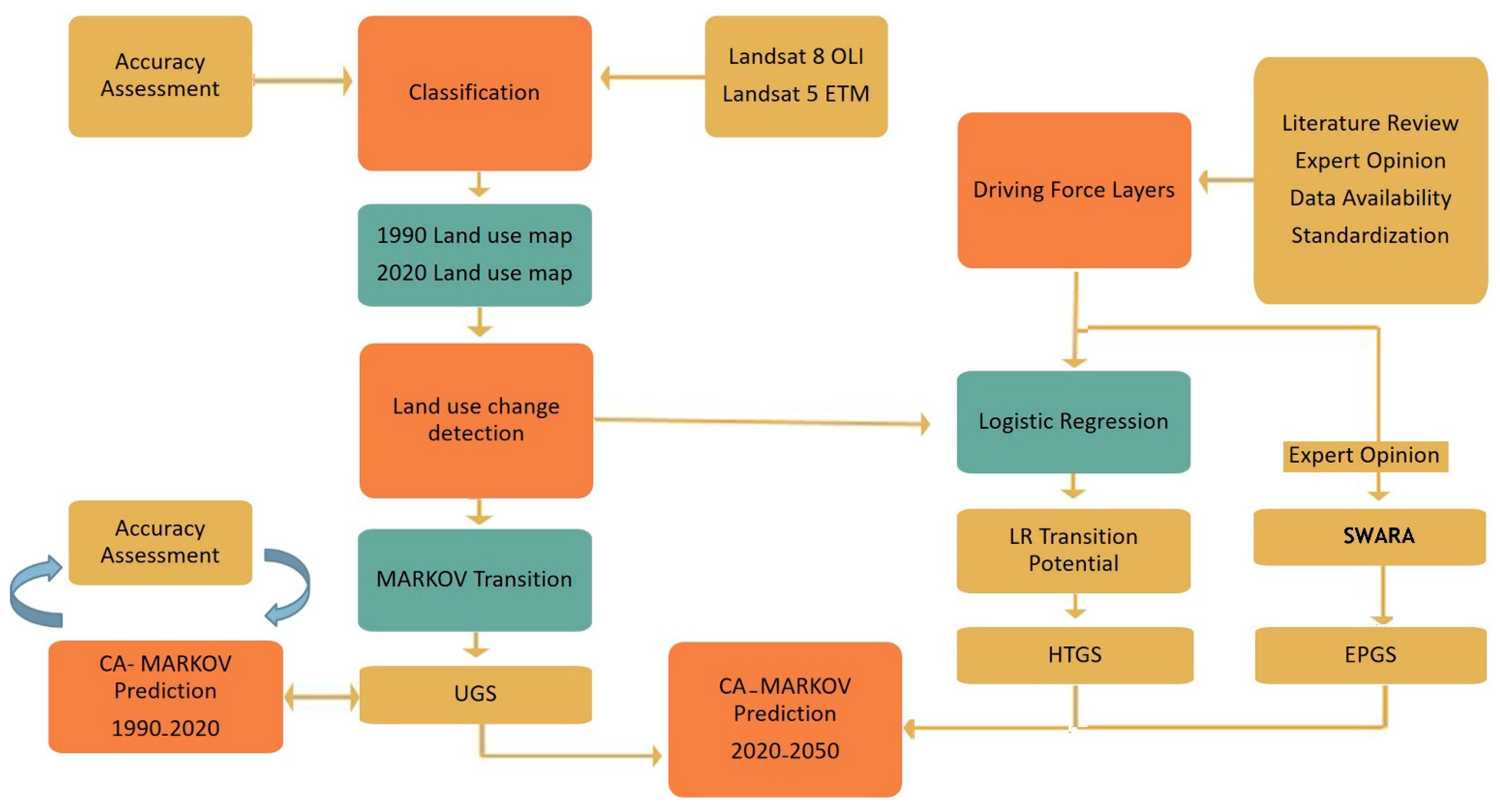
3. Materials and Methods

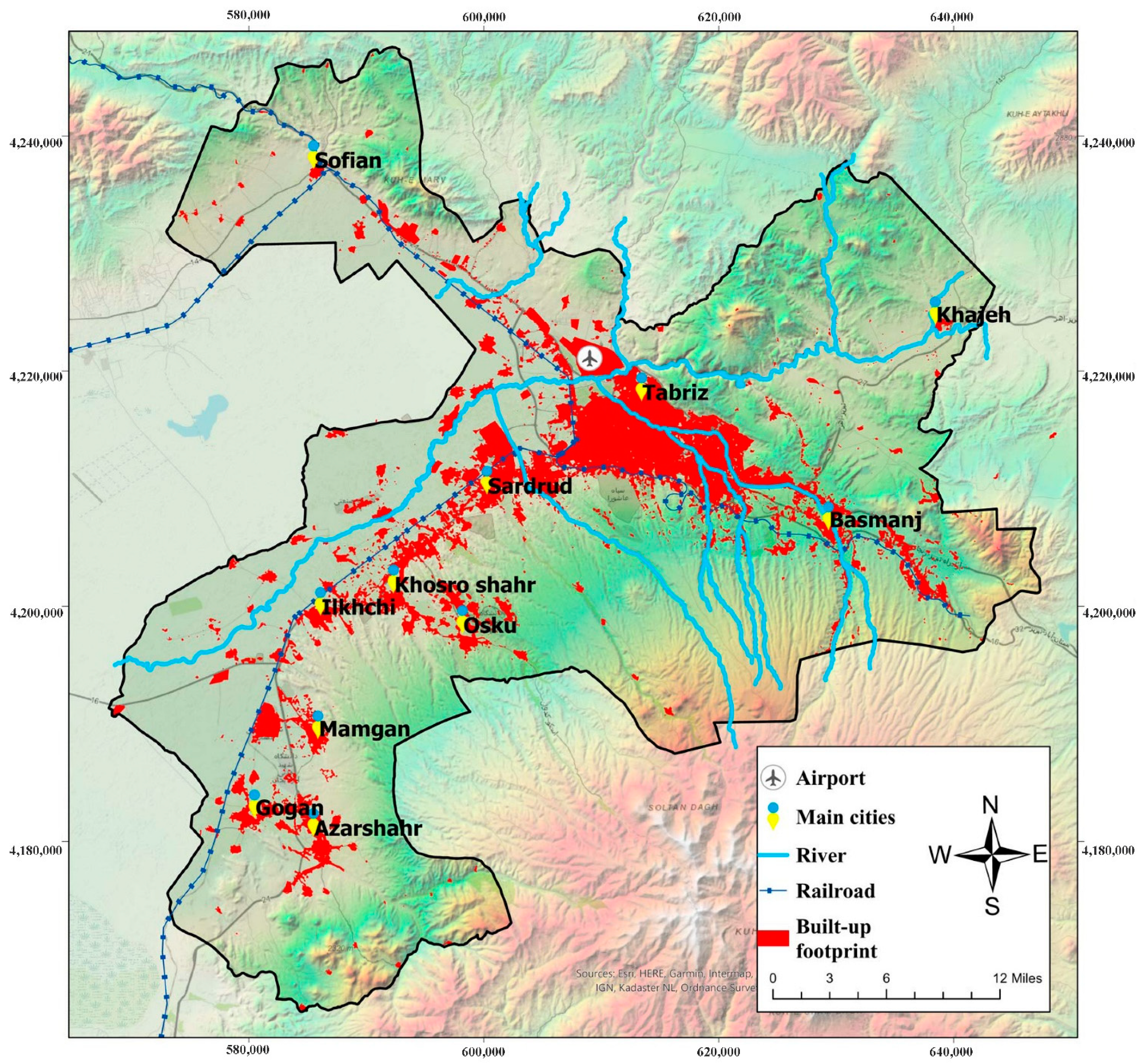
The general steps of the research include preparing the data, determining the driving forces, setting the growth scenarios, modelling the changes through the CA-MARKOV model, and finally analysing the results of the scenarios, which are shown in Figure 1.

3.1. Study Area

The study area is located in East Azarbaijan province and serves as this region’s political and economic hub. This region is the largest metropolis in northern Iran and is 1340 m above sea level. The region is divided into six counties: Osku, Azarshahr, Bustanabad, Tabriz, Shabester, and Heris, 12 cities, and 133 villages [93]. In recent years, the TMA, known as the hub of capital, employment, and population in the country’s northwest, has experienced a variety of changes in population, housing, and job trends. Extending industrial centres in urban zones such as TMA has been a goal of Iranian national and municipal programmes and plans since at least the 1970s. Most planners and policymakers have urged the establishment of new industrial estates around regional centres, the majority of which are situated in ecological and protected zones, in order to meet the growing land/space demand brought on by the remarkable rate of urbanisation. Typical farming, animals, the environment, and natural resources are all negatively impacted by the accelerated degradation of land caused by this trend. The city’s quick population expansion and influx of new residents may be directly attributed to the availability of jobs and a wide range of other conveniences and services. Tabriz has a strong monocentric core, which works as an absorbing pole to the main concentration of activity due to the city’s excessive economic concentration. Most economic activity and employment in TMA take place in the service sector; the industrial and agricultural sectors are broken down into the following subsectors [94]. The city of Tabriz is home to a sizable chunk of this population.

Nonetheless, there has been a considerable increase in the number of people living on the fringes of urban regions in the previous decade, suggesting that land use, urbanisation, and landscape patterns have undergone major shifts. This kind of unrestrained development has disrupted land-use patterns and upset the ecological harmony of the area. The TMA has expanded at an alarming rate as agriculture gives way to industry and services and as natural areas are wiped off.

Table 2. Population and built-up area change from 1990 to 2020 [93,94].

Year	1990	2000	2010	2020
Population	1,121,282	1,370,757	1,722,168	1,878,906
Built-up area (hectares)	13,530.3	21,393.4	29,635.8	35,352.2

shows that the study area’s population and built-up area have increased significantly over the last three decades. However, while the population has grown approximately 1.68 times between 1990 and 2020, the built-up area has increased by over 2.5 times, indicating a rapid expansion of the built environment in TMA. Figure 2 shows the area of the Tabriz metropolitan area.

3.2. Preparation of Land Use Data

Periods between 1990 and 2020 were selected to study the past land changes trend. For this purpose, Landsat 5 TM and Landsat 8 OLI satellite imageries were obtained from the USGS (United States Geological Survey) database with a spatial resolution of 30 × 30 m. Then, geometric corrections were made on the images obtained in the ENVI 5.3 software environment, and the maps were accurately geo-referenced. To specify the extent of the study area, the political boundary was used based on the Tabriz urban complex plan related to 2005, which was obtained from Tabriz municipality. The Digital Elevation Model (DEM) for slope preparation was obtained from the USGS organisation database. Then, to prepare the land use map, six land use categories were defined: cultivated land, garden land, built-up land, grassland, watershed, and bare land. The supervised classification method and maximum likelihood classification algorithm were performed in ENVI software based on a user-defined classification series. Then, to remove single pixels and unwanted errors, we applied the majority filter with a 5 × 5 window to the classified images.

Accuracy Assessment

The accuracy assessment compares classified images with reference images or ground truth data that is thought to be correct. Following land use classification, it is essential to evaluate the accuracy of these classification compatibilities with real-world images. Therefore, an accuracy assessment estimates the quality of a classified land use map. The Kappa coefficients ranging from 0.55 to 0.70 imply a good agreement, 0.70 to 0.85 indicate a very good agreement, and values more than 0.85 show an excellent agreement between the image and the ground [95].

The ENVI’s “confusion matrix” algorithm evaluates the accuracy of reference images. Based on the user-controlled area, an accuracy assessment corresponding to 10% of the land cover classes was developed. This method captures reference areas from all classes at a given rate and validates the correctness of the results. Different methods are applicable to select reference sample locations. Nevertheless, for this research, Google Earth and Landsat satellite images are employed to collect reference sample areas from different time periods. Equations (1) and (2) show the equations used for estimating assessment accuracy [95]:

$$Kappa=\frac{\mathrm{N}{{\displaystyle \sum }}_{i=1}^{r}xii-{{\displaystyle \sum }}_{i=1}^{r}xi+\ast xi+1}{N^2{{\displaystyle \sum }}_{i=1}^{r}xi+\ast xi+1}$$

(1)

$$Kappa=\frac{\left(\mathrm{Total}\mathrm{sum}\mathrm{of}\mathrm{correct}\right)-\mathrm{Sum}\mathrm{of}\mathrm{the}\mathrm{all}\mathrm{the}\left(\mathrm{row}\mathrm{and}\mathrm{column}\mathrm{total}\right)}{\mathrm{Total}\mathrm{squared}-\mathrm{Sum}\mathrm{of}\mathrm{the}\mathrm{all}\mathrm{the}\left(\mathrm{row}\mathrm{and}\mathrm{column}\mathrm{total}\right)}$$

(2)

The Kappa index was calculated as 75% for the land use map of 1990 and 87% for the land use map prepared in 2020, which according to similar studies, shows an acceptable ratio [96,97].

3.3. Measuring the Driving Forces of Land-Use Change in TMA

In recent decades, Tabriz metropolitan area has witnessed significant land use change due to underlying factors such as biophysical, socioeconomic, and political [4]. We collected secondary data on the potential factors, especially those affecting urban growth. Sixteen factors were finalised by taking advantage of experts’ opinions and considering local specific conditions.

Table 3. The selected driving forces and their measurement.

Theme	Sub-Theme	Factors	Unit	Suitability Level (Standardised)
Bio-physical		Slope	Percentage	Slope class between 0–5%—suitability level = 255 Slope class between 5–10%—suitability level = 150 Slope classes between 15%—suitability level = 75
		Land cover	Categorial	irrigated lands = 0 urban lands = 255 orchard lands = 25 agricultural lands = 50 rangelands = 100 barren lands = 255
		Flood	Categorial	flood-prone areas = 100, Other areas = 255
		Fault	Meter	Based on the Euclidean distance (in meters) from the maximum distance (255) to the minimum distance (0), which suitability increases uniformly with increasing distance
		Earthquake	Categorial	Suitability of high-risk zones = 100 Suitability of medium risk zones = 150 Suitability of low-risk zones = 255
		Elevation	Meters	The degree of suitability of heights between 1200–1500 = 255 Suitability of heights between 1500–1900 = 100 heights between 1500–1900 = 20
Human	Accessibility	Access to educational centres	Meters	Based on the Euclidean Access (in meters) from the highest access (255) to the lowest access (0), which decreases uniformly with decreasing access
		Access to entertainment centres	Meters	Based on Euclidean Access (in meters) from maximum access (255) to minimum access (0); suitability decreases uniformly with decreasing access
		Access to the transport network	Meters	Based on Euclidean Access (in meters) from maximum access (255) to minimum access (0); suitability decreases uniformly with decreasing access
		Access to major cities	Meters	Based on Euclidean Access (in meters) from maximum access (255) to minimum access (0); suitability decreases uniformly with decreasing access
	Socio-Economic	Land Price	Categorial	Class 1: 255 Class 2: 150 Class 3: 50
		Population density	People per hectare	suitability increases from 0–255 based on increasing population density of major cities
	Specialised planning regulations	Rivers	Meters	suitability at a distance of 0–250 m = 0 suitability at a distance of 800–250 m = a uniform increase between 0–255 with increasing distance suitability at a distance of 800 m and above = 255
		Ecologically protected lands	Categorial	suitability of ecological areas = 20 Other areas = 255
		Industrial buffer zone	Meters	distance of 0–350 m = 0 distance of 1000–350 m = uniform increase between 0–255 with increasing distance distance of 800 m and above = 255
		Existing mines	Meters	suitability in the range of mines = 0 suitability at a distance of 0–500 m = a uniform increase between 0–255 with increasing distance suitability a distance of 500 m and up = 255

details the selected driving forces and their categorisation for urban growth suitability.

Each factor is scored based on its potential function in the competency for urban land use change. It quantifies each component and is converted into spatial layers in ArcGIS (Arcmap) version 10.3 using the fuzzy standardisation method (range 0 = lowest suitability—255 = highest suitability). The data were obtained from Tabriz municipality in 2021. The final output of the preparation of LUCC factors is evaluated and standardised in Figure 3. The degree of suitability of each factor in affecting land-use change is displayed.

3.4. Calculation of Markov Chain (MC) Transition Probability and Uncontrolled Growth Scenario (UGS)

MC modelling is a simulation technique used in land use analysis. ‘Markov’s analysis of land-use change is combined with GIS to provide a tool for visualising and predicting land-use change likelihood across land-use classes. Markov variations have been frequently used in modelling land changes [45,53,71]. MCs are stochastic models that show how a process may transform from state A to B. The principal part, the transition likelihood matrix, stands for these changes. This matrix is used to calculate projections of the area of LUCC in state B. The transition area matrix estimates the areas (pixels) transferred between states A and B and is another output of MC. An earlier study [53] documented the detailed description of MC and its implementation. Based on the land use maps from 1990 and 2020, the MC model calculates the LUCC transition area matrix and the transition probability matrix. Markov analysis is the input of the CA–Markov prediction model and is considered the calibration stage of this model; it is necessary to evaluate the stability of findings before proceeding to simulations. Thus, we used a past to present (1990 to 2020) simulation to ensure the calibrated matrix accuracy and validation of its prediction results. The results of the MC were tested in a scenario called UGS. This scenario seeks to predict the future land use status by 2050 based on the trend of its historical changes. In other words, the aim is to examine how the LUCC will evolve by 2050 if conditions are based on historical trends and based solely on the conversion rates between land use classes. The LUCC transition area matrix and the transition probability matrix are used as transition rules in the CA–Markov model to predict future growth using TerrSet in this scenario. The layers used in this scenario are the raster layers produced by the MC, which shows the potential for land conversion between land use classes and the land-use layer of 2020 as the base year.

3.5. Logistic Regression (LR) and Historical Trend Growth Scenario (HTGS)

LR has been used as an experimental model in deforestation analysis, groundwater potential, agriculture, landslide probability mapping, and urban growth modelling [4,15,53,56,98]. The LR is such that it considers several explanatory factors as independent (X) variables and measures their association with a dependent variable (Y). The dependent variable, Y, takes a binary value of 0 or 1. The value of 1 shows that the event occurred, while the value of 0 indicates the event did not occur. Therefore, the equation obtained from LR is as Equation (3):

Logit (p) = ln (p (1 − p)) = a + (b1 × X) + (b2 × X2) +(b3 × X3) + … (bn × Xn)

(3)

where p is the dependent variable expressing the probability of becoming 1; X is the independent variable, … xn, x2 and x1 are independent variables, and a is the constant of the regression equation. b3 … bn, b2, b1 are the coefficients of each independent variable. The relationship between the dependent and independent variables goes along with a logistic curve. The maximum likelihood function estimates the significance and coefficient of each explanatory variable. The reflection of LUCC in each cell (raster image pixel) can be binary: changed (= 1); not changed (= 0). It is assumed that the probability of change of each cell based on the logistic curve is as in Equation (4):

$$f\left(z\right)=\frac{1}{1+e^{-z}}$$

(4)

The probability that the raster network cell will change is described based on Equation (5):

$$P\left(Y=1/X_1,X_2,X_3,\dots \right)=\frac{1}{1+e^{-\left(\alpha +{{\displaystyle \sum }}_{i=1}^n{\beta }_i{X}_i\right)}}$$

(5)

The LR model is used to determine the power and significance of each variable in LUCCs during the study time period. Before implementing the LR model, sub-models should be identified. Each of the sub-models represents a change from one land class to another. In this study, four sub-models, including gardens to built-up, cultivated to built-up, grass to built-up, and barren lands, are defined (the watershed sub-model is not considered because it had no significant changes). Then, the impact of each variable on the conversion of sub-models is calculated. The role of the driving forces in LUCC concerning urbanisation is determined. First, the layer of changed zones is entered as the response variable, then the layers of driving forces (Figure 3) are entered as explanatory variables. Each sub-model contains coefficients as the impact of each factor in LUCC (Table 3).

This scenario is known as HTGS, where the goal is to involve the driving forces of LUCC in terms of urbanisation. This scenario investigates what role the driving forces of LUCC have had in the past, furthermore, how they will impact the future of LUCC patterns. The Weighted Linear Combination (WLC) method overlapped the layers created in Figure 3 and retrieved a layer of LUCC potential in the TerrSet software environment. A probability layer of LUCC was prepared to multiply coefficients of explanatory factors and then overlay driving force layers. In the WLC step, the values obtained from LR for each factor were regarded as coefficients of importance.

3.6. Multi-Criteria Evaluation (MCE) and Environmental Protection Growth Scenarios (EPGS)

The EPGS strives to predict future growth in order to preserve the environment and prevent the loss of valuable agricultural and ecological assets. This scenario seeks to investigate how the experts’ knowledge and insight can be involved in simulating future changes and how the effects of urbanisation on future land-use changes can be controlled. The MCE method is used because the effect of each factor on the degree of environmental protection should be figured out in comparison with other factors. We used the Stepwise Weight Assessment Ratio Analysis (SWARA) method. The SWARA method involves two important steps: the first is to prioritise the criteria by consulting experts, while the second is the weighting process. The SWARA method involves considerably lower pairwise comparisons and is easy to use compared to other popular methods, such as the AHP [99,100]. The mathematical expression for determining the integrated weight of the attributes is as in Equation (6) [99]:

$$\overline{w}=\frac{w_j^{*}{w}_j}{{{\displaystyle \sum }}_1^n{w}_j^{*}{w}_j}; {\displaystyle \sum }_{j=1}^n\overline{w}=1,2,\dots ,n,$$

(6)

where $w_j^{*}$—objective weight of the j attribute; $w_j$—subjective weight of the j attribute;$\overline{w}$—integrated weight of the j attribute (please see [101]).

In this method, the experts and policymakers of TMA were asked to compare each of the drivers of LUCC listed in Table 3 with others to get a sense of their relative importance in targeting sustainability. To this end, the questionnaire, including the criteria, indices, and scoring system, was sent to 32 experts with high education (masters or above) considering a mixed job and qualification status (

Table 4. Background information of experts.

		No.
Field of expertise	Environmental science/Ecology/Geology/Geographer	5
	Urban & regional planning/Rural planning	7
	Urban management/Public policy	4
	Economics/Finance/Accounting	6
	Civil engineering/Hydrology/Water engineering/Surveying	7
	Sociology/Demography	4
Gender	Female	9
	Male	23
Years of experience	Less than 10 years	14
	Over 10 years	18
Educational Level	Masters	23
	Ph.D.	9
Employment sector	Government/Public/Public-private	21
	Private	9
	Self-employment	2
Total	NA	32

). However, only 12 experts responded on time, with a response rate of 37 per cent. After determining the final weights of the criteria (see Table 4) using the SWARA method, the WLC method was used to overly the layers prepared in Figure 3 and turn them into a potential layer in the TerrSet.

3.7. Predicting and Simulating Changes with the CA

CA-based models have been widely used in urban expansion simulations [31] because they show the transmission capacity of complex spatial processes, such as displaying diverse local behaviours with global patterns [102]. In addition, the complex behaviour of systems can be simulated and demonstrated by developing transfer rules in CA models [102].

The CA segment of the LUCC model determines land-use allocation in each cell. CA models define the new land-use status of each cell over a distinct time period. The change is defined by a set of exact rules that precede the implementation of this procedure. The execution of automated cells is based on a cellular space, a neighbourhood definition, a number of cases, and a set of transfer rules [103]. The most critical step in CA modelling is the definition of transformation rules based on the training data that control the model. Nevertheless, land-use dynamics are highly complex, requiring non-linear bounds to define laws, despite using linear bounds for defining the rules [46].

Integrating the CA model with other simulating platforms is an effective way to overcome the constraints of an older model such as SLEUTH [46]. CA-MC integrates a deterministic modelling framework with a stochastic, time-based framework as a hybrid modelling technique that links linear spatial strengths [53]. The model is created by integrating MC and CA models. It is a robust way to simulate spatial dynamics and forecast future land use change based on the historical pattern. Hence, this approach using a CA function can turn MC results into objective spatial outcomes [102]. Furthermore, some studies merge CA and LR models in order to examine the model’s validity [46].

4. Results

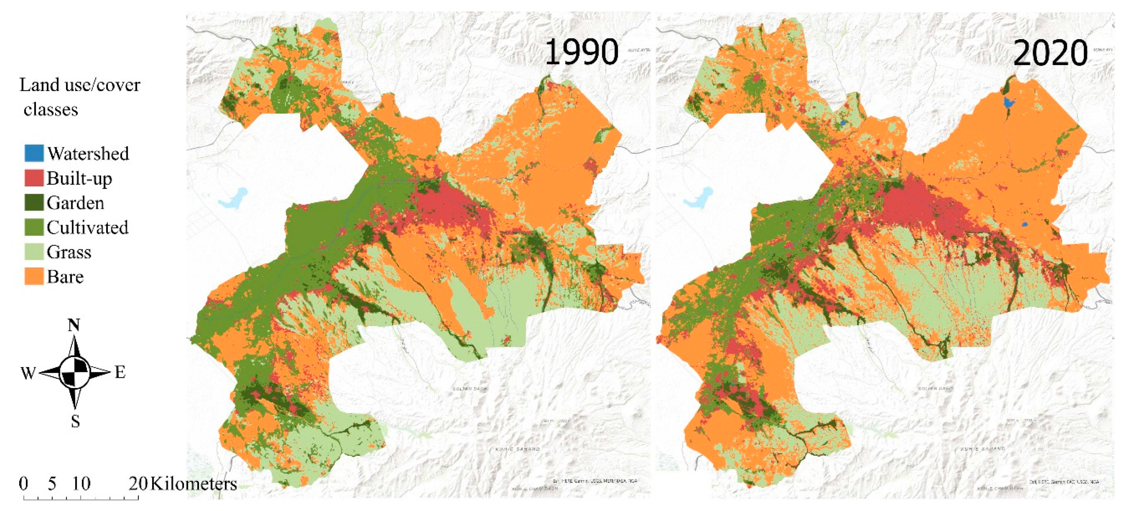
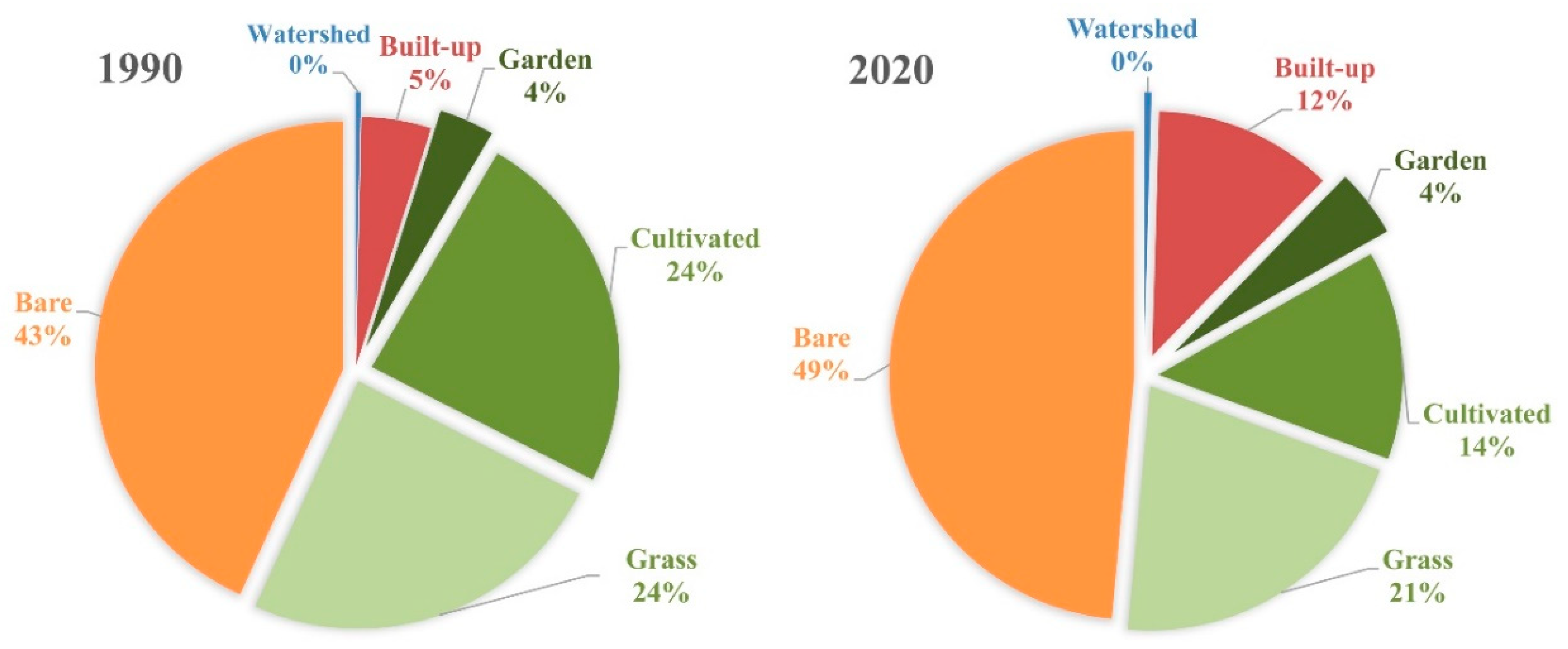
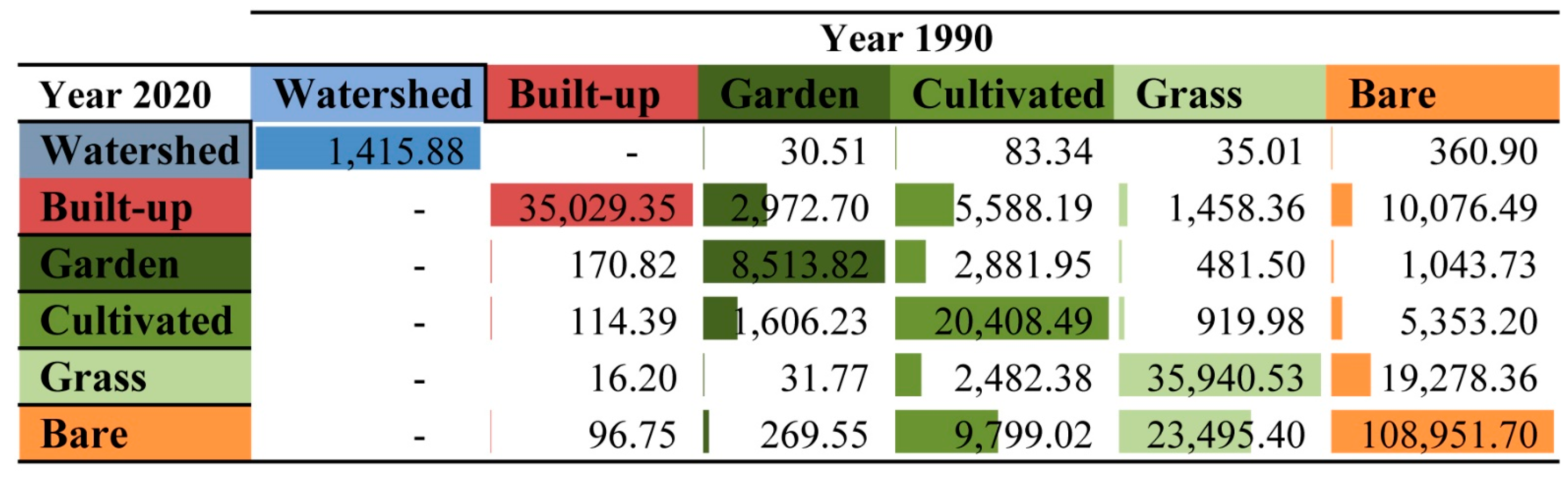
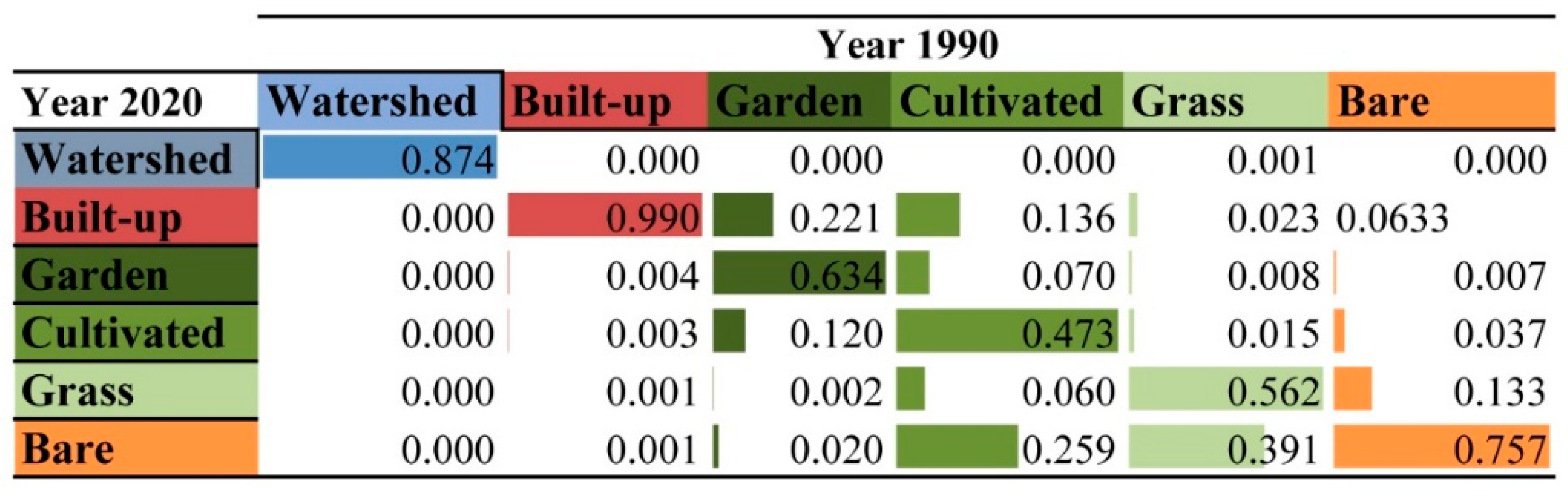
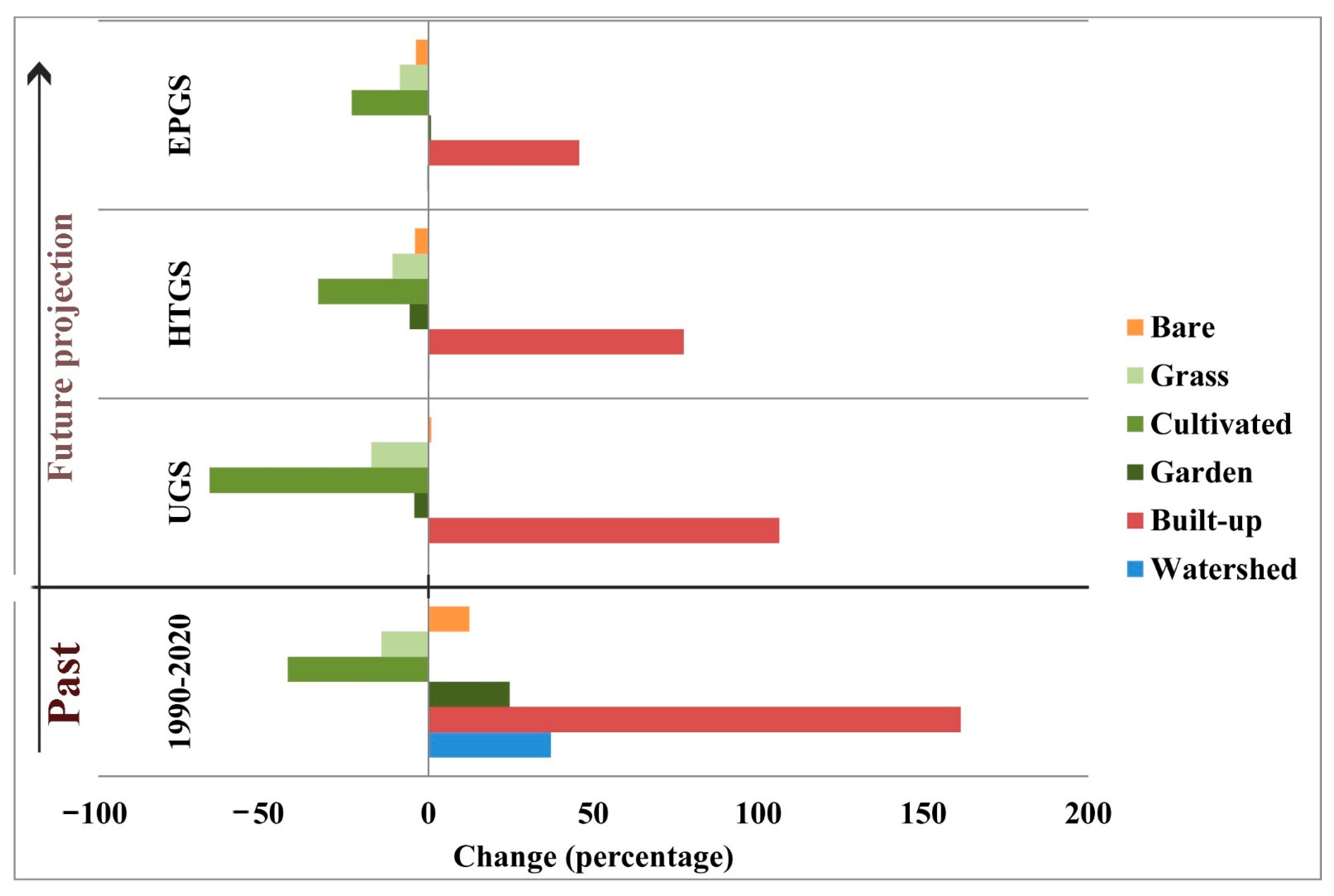
4.1. Detecting LUCC in the 1990–2020 Period

After classifying the satellite photos and confirming the outputs for TMA, the results are shown in Figure 4. This time period spans from 1990 to 2020. Visual inspection reveals that the TMA’s north and northwest have received heavy LUCC. By 2020, much of the cultivated land in these regions had broken up into smaller and smaller plots. As a result, natural features were more isolated from the expanding urban regions. Additionally, human activities led to the dispersal of human settlements and urban regions throughout the metropolitan landscape. These places are concentrated mostly in close proximity to major cities. It has been mostly concentrated in the western and northwestern portions of TMA.

Figure 5 shows that from 1990 to 2020, the proportion of built-up land increased, whereas the proportion covered by cultivated, grass, and bare land dropped. Figure 5 shows that the proportion of the built-up has increased from 5% to 12%. Over the same time period, the proportion of cultivated fell by around 10%. Additionally, throughout this time period, bare land declined from 49% of the overall share to 43%.

It is essential to know about inter-class exchanges after analysing the LUCC’s composition and configuration pattern. Determining changes such as net decrease or rise, variation within each class, and movement across classes are all instances of change detection. TerrSet was able to discover this by comparing LUCC results from 1990 and 2020. (Figure 6). According to the findings, the highest rate of land classification shifts occurred in the cultivated category. The most notable shifts occurred when cultivated land was transformed into a built-up area (5588.19 hectares) or into bare land (9799.02 ha). Between then and now, 19,278 hectares were transformed from bare to grassland. However, the built-up areas saw tremendous growth due to the transformation of other classes. The majority of cultivated was turned into built-up. In addition, 10,076.49 hectares of bare land and 2972.7 hectares of garden land were transformed into an urban setting.

Results from the MC study pinpoint LUCC behaviour. The reasoning for modelling future probabilities is embodied in these transition potentials and transition areas. Figure 7 suggests that conversion of garden and cultivated land to urban use occurred most likely. On top of that, most likely, cultivated land was being converted to bare land or built-up area. It indicated that there was a high potential for converting cultivated into the aforementioned area. Furthermore, the transition from grassland to bare land accounted for the vast majority of the movement.

4.2. LR Coefficients of Driving Forces

The results of LR are shown from 1990 to 2020 in

Table 5. Results of LR in estimating the potential of changing non-built-up to built-up lands.

Theme	Sub-Theme	Factors	Garden to Built-Up	Cultivated to Built-Up	Grass to Built-Up	Bare to Built-Up	Standardised LR Coefficient	SWARA Coefficient
Bio-physical		Slope	0.0005	0.006	−0.0032	−0.0013	0.0919	0.1301
		Land cover	−0.0821	−0.0243	−0.0137	0.0027	0.0817	0.1981
		Flood	0.0079	0.0032	0.008	0.0043	0.0616	0.0571
		Fault	−0.0022	0.0024	−0.0016	0.0000	0.0567	0.0851
		Earthquake	−0.0036	0.0054	0.0030	0.0037	0.0823	0.0121
		Elevation	0.0126	0.0232	0.0015	0.0065	0.0202	0.0541
Human	Accessibility	Access to educational centres	0.0021	−0.0037	0.0038	0.0006	0.0269	0.0131
		Access to entertainment centres	0.0352	0.0151	0.0297	0.0164	0.0564	0.01501
		Access to the transport network	0.00024	0.0158	0.0082	0.0139	0.2063	0.1301
		Access to major cities	0.0289	0.0000	−0.0019	0.0007	0.1058	0.0101
	Socio-Economic	Population density	0.0008	0.0022	−0.0009	−0.0032	0.0713	0.0401
		Land Price	0.0081	0.0068	0.0136	0.0079	0.1969	0.0221
	Specialised planning regulations	Rivers	0.0121	0.0058	0.0072	0.0044	0.0122	0.0741
		Ecologically protected lands	−0.0011	0.0004	0.0001	0.0009	0.0112	0.1091
		Industrial buffer zone	−0.0041	−0.0039	−0.0038	−0.0014	0.105	0.0381
		Existing mines	0.0026	0.0023	0.0020	0.0027	0.0116	0.0131
Model output descriptors
		Adjusted odd ratio	37.5032	42.5096	48.8362	17.2894
		True-positive (%)	98.6030	98.6030	90.9090	98.5310
		False-positive(%)	0.2000	0.7111	0.2492	1.0861
		ROC	0.9940	0.9790	0.9710	0.9320

. For each of the four existing sub-models, the coefficients of each independent variable are determined. Coefficients that go closer to one indicate a stronger relationship between the variable and the rate at which undeveloped land is developed. As a result, negative coefficients illustrate the opposite relationship between variables. Table 5 shows that the coefficient of 0.0352 for proximity to entertainment places is a major factor in the transformation of gardens into built-up areas. Additionally, access to the transportation network has drastically transformed cultivated land into built-up areas (with a coefficient of 0.0158).

The land cover variable is also the most significant barrier to the transformation of rural regions into urban centres. The LR method’s precision was measured using the ROC index. Table 5 shows that there is a significant relationship between the transitions and variables throughout both scenarios and across all sub-models, at a significance level of 0.9 or above, validating the model.

According to Table 5, elevation was one of the essential variables, indicating that the urban land begins to occur at a lower altitude and then expands to height. Furthermore, accessibility to entertainment centres and accessibility to transportation networks has had the most significant impact on built-up land development. On the other hand, the two variables of land cover and population density worked against built-up land development. As expected, closeness to hazardous zones such as floods and faults had a significant role in future development.

4.3. Results of the Spatial Simulation

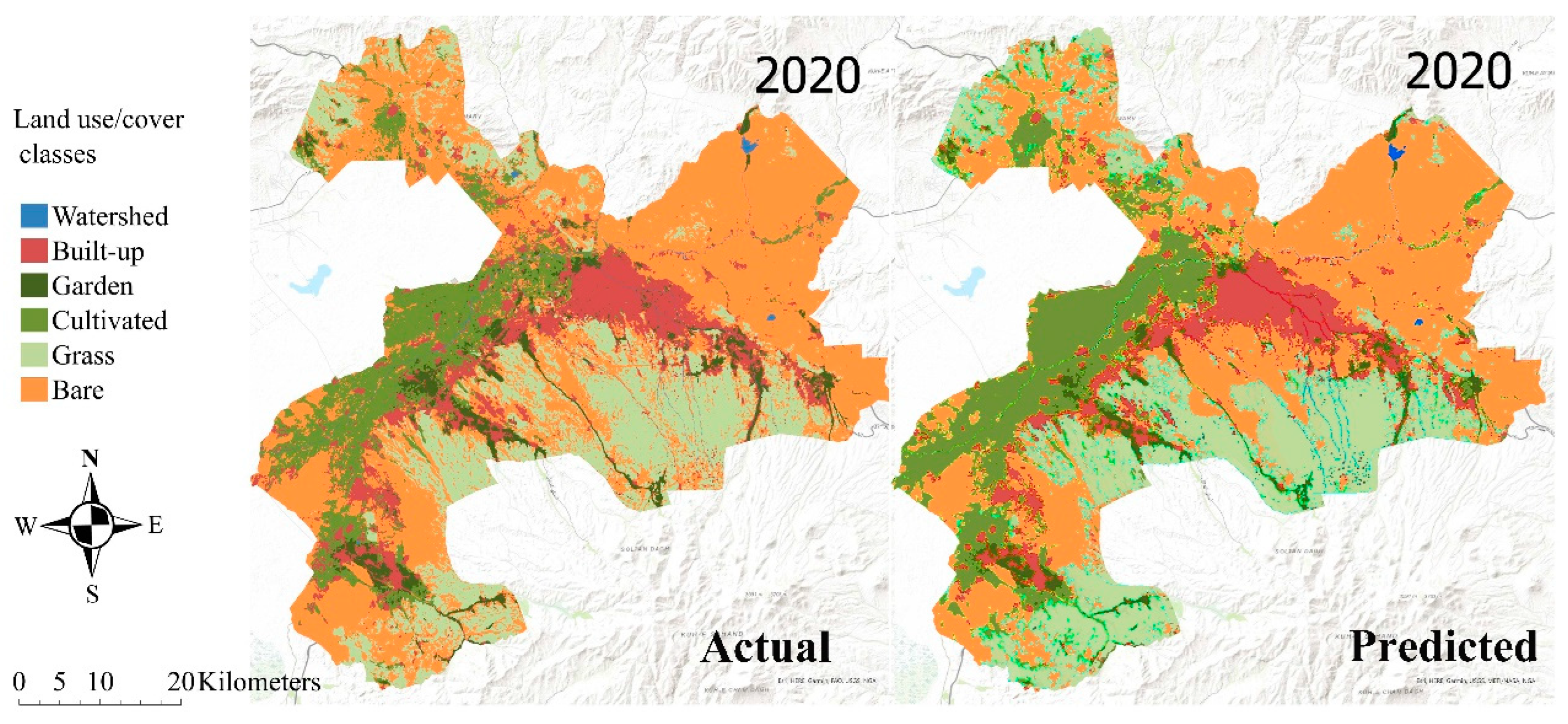
4.3.1. Validation and Experimental Prediction Results

The validation of LR maps was carried out using the ROC method (Table 5). ROCs greater than 0.9 for all types of land uses show high accuracy in explaining LUCCs. The outputs of Markov analysis and the base map of 1990 were used as the inputs of the CA_MARKOV model. Furthermore, the LUCC from 1990 to 2020 were simulated. The results of the 2020 simulation based on the Markov analysis are shown in Figure 8. The results of the 2020 simulation show the accuracy of the Markov analysis in recording the changes evaluated with the 2020 reference map. The Kappa coefficient method was used to validate the model’s prediction accuracy. The calculated kappa coefficient was 70%, which indicates an acceptable value. Land changes by 2050 can be predicted with 70% accuracy.

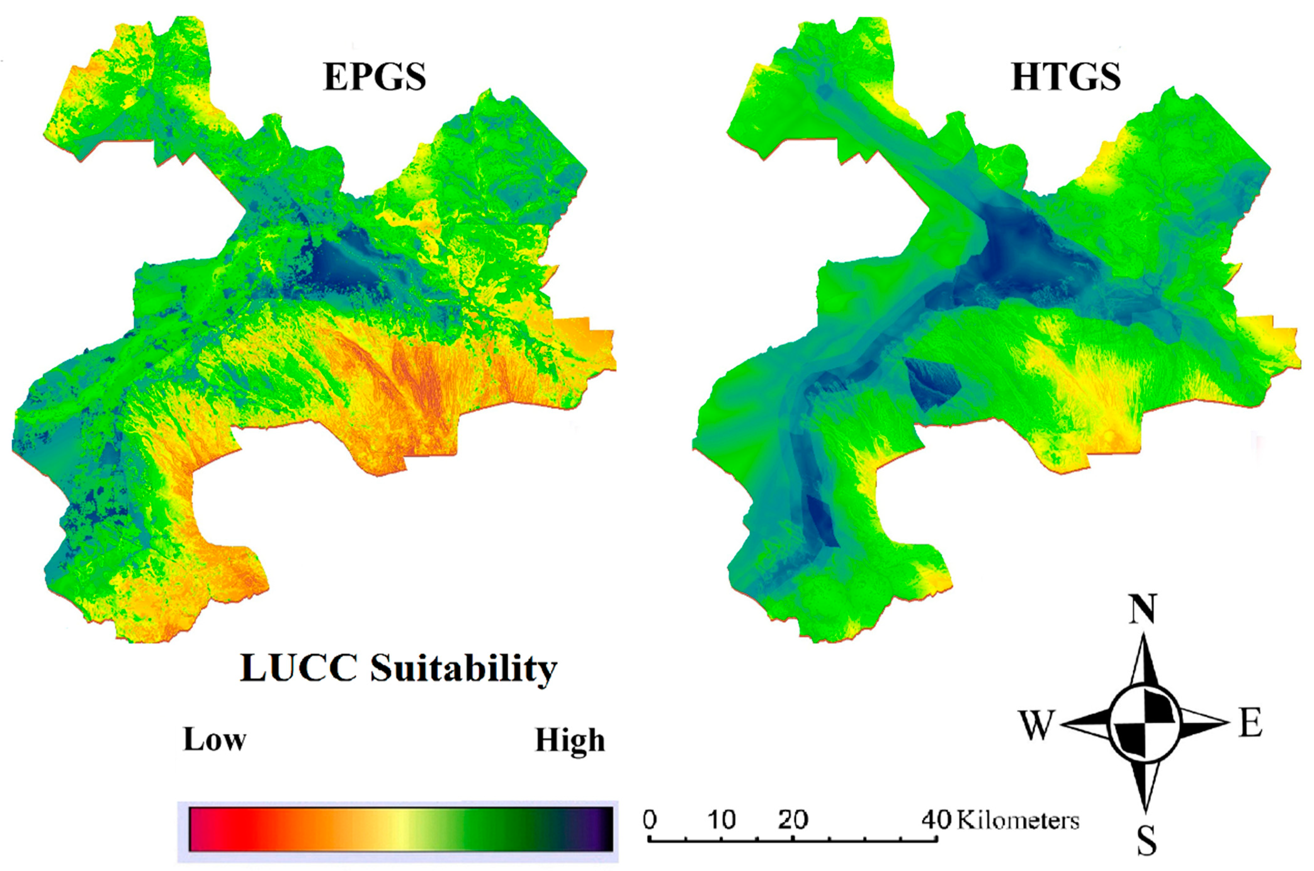
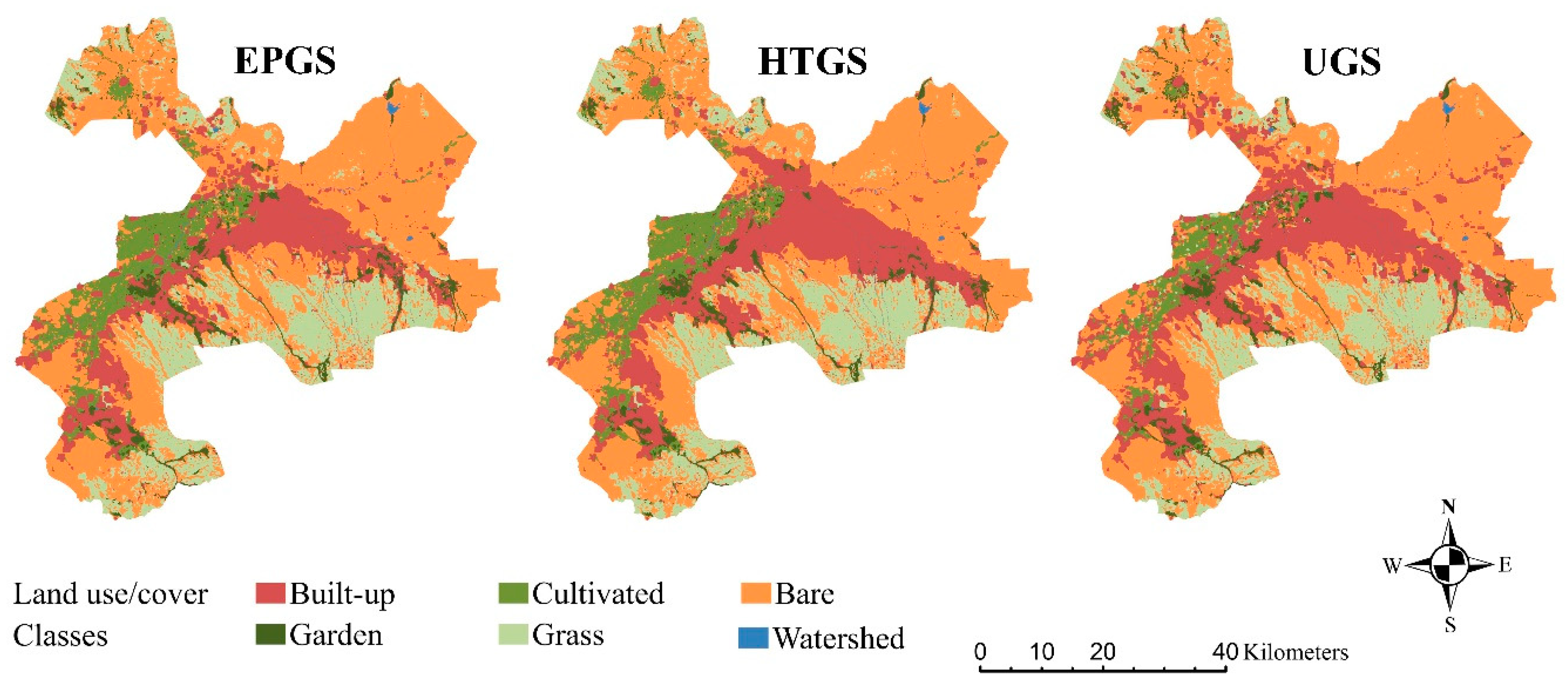
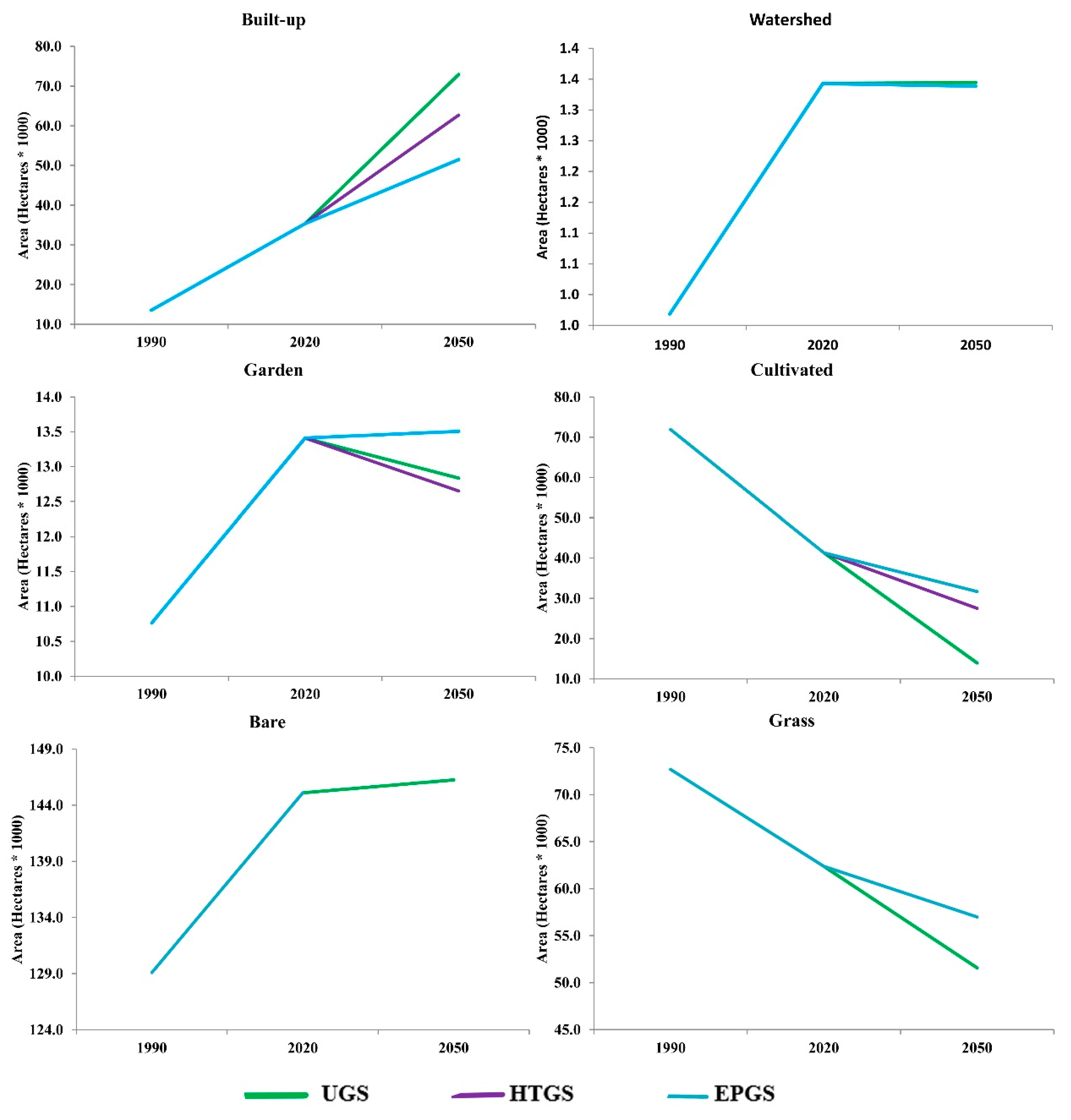
4.3.2. Results of the Spatial Simulation of Scenarios up to 2050

Using the LR model’s prospective transmission maps, MCE expert assessment, and CA model transition rules, we constructed scenarios for their geographical implementation. Figure 9 depicts the possibility for convergence between land use/cover maps under the HTGS and EPGS scenarios. As a whole, it is clear that HTGS has more promise for LUCC. This will happen mostly in and around major cities and along major transit corridors. In addition, LUCC is more prevalent in the TMA’s central and northwest regions. The potential of LUCC is limited when applied to EPGS, which suggests that in the future, LUCC will only occur in places immediately adjacent to existing urban centres and that LUCC will have a far less impact on the natural environment than HTGS. The biologically protected and high-elevation regions in the north and northwest of TMA mean that the south parts have less LUCC potential.

TerrSet employs the CA–MARKOV to model the LUCC of TMA in the future under three predetermined scenarios by the year 2050. The results of these simulations for all three 2050 scenarios are shown in Figure 10. The proposed scenarios predict that by 2050, each kind of land use or cover will have a unique geographic position. Overall, TMA will contain a lot of LUCC if Figure 10 is any indication. In general, it seems that the TMA landscape configuration will undergo significant change. The massive growth of cities has made it such that LUCC are most common around their borders. Fast urbanisation and rural sprawl, together with a decline in cultivated and grass lands, characterise the period from 2020 to 2050. The findings suggest that TMA’s extensive urbanisation process from the past may be expected to continue into the future. Mainly in the north, northwest, and west of the TMA, where Tabriz, Azarshar, Heris, and osku are located, you will find areas with high rate of LUCC. Land situated between urban and rural regions is being demolished and developed into residential, industrial, and service districts, and this process is becoming increasingly obvious. This pattern will also be seen along the major thoroughfares that link major cities. The northwest area of TMA, where most cultivated and garden land is located, experiences a sharp decline in the scenarios, leading to the loss of many precious resources. In particular, the urban core, the east-west axis, and the Tabriz-southeast axis will grow and merge, while most of the city’s dispersed villages will link with one another. Figure 10 reveals that HTGS has higher levels of LUCC than other scenarios, with the greatest increases seen in the periphery of urban areas and in Tabriz itself. Further, EPGS has more densely populated areas and lower LUCC. There will be less degradation of precious landscapes and a more limited urban footprint in this scenario. However, under the UGS scenario, LUCC would happen fragmented due to the conversion of cultivated land.

Analysing the composition of TMA indicate that this landscape will be home to significant LUCC in the future. Figure 11 displays the results of a change detection analysis, which shows that general trends are consistent across all three scenarios. The scenarios all predict significant growth in urban areas, consistent with historical patterns; however, the rate of growth in the UGS is expected to be much higher than in the HTGS and the EPGS. The pattern of cultivated land conversation is similar, but opposite. Continuing on the downward trajectory shown in the scenarios leading up to 2050, we expect the largest decreases in UGS, HTGS, and EPGS respectively. Figure 11 shows that grass land is expected to move in the same direction as cultivated land. Contrary to the historical trend, both UGS and HTGS will decrease even while garden areas continue to grow. Nonetheless, the rate of expansion will remain slow relative to historical norms. The barren terrain and watershed continue on a trajectory similar to that seen in the past but with a more constant line going forwards.

Figure 12 depicts the aggregate pattern of changes over all three scenarios, showing an increase in developed regions and a decrease in undeveloped territory. There are major variations in predicted LUCC growth rates across the three scenarios. The percentage of built-up land will increase dramatically (106%) in the UGS. For HTGS, the equivalent figure will be about 77%, whereas, for EPGS, it will be around 45%. UGS projections predict that the area of cultivated will drop by −65%, indicating widespread devastation. For HTGS, this equates to a −33% reduction, and for EPGS, it will be about a −25% reduction. In contrast to the other two situations, LUCC in the EPGS has the lowest ratio. The EPGS see a rise in urban areas by 45%, although the negative growth of cultivated and grasslands will be lower than in any other scenario. In addition, the garden areas will fully preserved in this EPGS.

5. Discussion

Using an integrated framework, this research examined the regional dynamics of LUCC and its driving mechanisms in TMA from 1990 to 2050 under several growth scenarios. First, between 1990 and 2020 in TMA, natural and cultivated lands were harmed due to the growth of urban areas, as shown by the findings of previous LUCC. Similar findings have been observed in previous research on LUCC in TMA [4,97]. Tehran [15,102,104,105], Karaj [106], Sari [7], Mashhad [107], and Isfahan [15] are only a few of the Iranian metropolises whose natural zones are threatened by urbanisation [108]. Furthermore, the LUCC geographical pattern reveals that most of the changes have taken place in the TMA’s north, west, and northwest, where industrial zones and working-class suburbs have been built mostly via edge expansion or leapfrog. New developed land is regularly expanded in close proximity to the already developed area; this is known as edge growth. Smaller human settlements and activities are spread out over the area in a leapfrog pattern. This shape is picked up in the areas northwest of TMA, close to the major highways and the places where agricultural and industrial activities take place. This result accords with previous results in the field of TMA [4,97]. Generally speaking, the growth of urban areas in Iran’s major cities is thought to be the primary cause of LUCC [44,57,63,104,109]. Grass, cultivated, and garden space all suffered as a result of the un-controlled expansion of cities. For effective management of LUCC and urban growth [51] in TMA, it is essential to analyse driving forces and implement scenario-based planning.

The LR model was used in this analysis because of its excellent accuracy and validity when looking at the factors that drive LUCC [15,39,46,78,110]. According to the results, cities have the most beneficial effect on LUCC by decreasing the amount of bare and cultivated land in the region. Thus, it is not surprising that urban centres spring up in proximity to transportation hubs. Figure 7 shows the high transition potential in TMA along the western axis (Tabriz Azarshar), northern axis (Tabriz Sofian), and southern axis (Tabriz Basmanj). Similar to the TMA, reports from throughout the world have shown that urban sprawl has occurred around major highways, indicating that the transportation network has a big impact on LUCC conversion as a result of human activity [44,51,62,72,98,111]. This research demonstrates the interesting connection between land price and LUCC, particularly via the urbanisation of once agricultural territory. This is because of the area’s closeness to human populations, where construction costs are often cheaper than in infilled-development regions. Access to metropolitan centres and built-up regions also influences the transformation of garden land. These places are being torn down due to edge development, which is causing the urban core to expand [4,9,15,60,98,112]. However, the majority of urban expansion has occurred in the periphery, not in the core or near the major metropolis. Most dispersed enterprises and settlements have grown in size and location around major thoroughfares throughout time. The closeness of industrial zones and slope have had a substantial detrimental impact on previous urban development. It was less expected that the TMA’s high slope areas, particularly those in the south and west where there are a lot of barren and grass fields, would be converted. Results from the LR show excellent effectivity and efficacy in this study, as they have in others when looking at the influence of driving forces and spatial dynamics of LUCC [15,46,53,110,112].

Three different scenarios were used to describe the LUCC dynamics in TMA. The Markov land conversion probability is an input to the UGS, which prioritises uncontrolled development. Using the LR model, the HGTS scenario examines the effect of LUCC’s driving factors. Expert perspectives on LUCC with an eye on preserving the environment are at the heart of the EPGS scenario. Predictions of LUCC for 2050 under each of the three scenarios show that urbanisation in TMA will continue to play a disproportionately large role. The expansion of urban areas and associated environmental degradation will occur mostly in UGS, where population densities are expected to rise to very high levels, and in EPGS, where urban growth is expected to occur in a more concentrated fashion. This implies that in the future, environmental deterioration will occur on a massive scale if we do not have a great understanding of the mechanisms that lead to LUCC and instead depend only on data that indicate the possibility for land cover type conversion. In the future, the landscape of TMA will consist mostly of built-up areas, which will lead to the loss of cultivated, garden, and grassland areas, which are among the most precious natural resources. Future situations will vary in how quickly this tendency unfolds. Cultivated and grasslands will contribute the least to the decrease in EPGS. The reduction will be accompanied by more deterioration in the UGS, and there will be no change in the amount of barren land or watershed. Consequently, urbanisation will have an impact on LUCC in the TMR. The projections based on the scenarios show that the EPGS will lead to beneficial effects on the cultivated and grass lands, and thus more sustainable LUCC, whereas the UGS would result in tremendous development of the built-up regions having detrimental consequences on the same fields. In reality, the EPGS emphasis on environmental protection as part of human development. Increased frugality and long-term resource management are the driving forces behind this situation. It makes the distribution of people and wildlife in the TMA landscape more equitable and sustainable. Evidence from China [41,54,67], Iran [4,15], Turkey [40], Latin America [6] and Europe [72] show that LUCC has occurred along major roadways and in the vicinity of existing cities, having a negative effect on the surrounding environment. The results demonstrate that the scenario method, which is represented by a variety of modelling outcomes for the year 2050, may provide decision makers with access to more viable alternatives [33].

The LUCC is often regarded as one of the most important planning concerns [113,114]. These results show that the complexity of LUCC makes it hard to simulate using a single model and set of assumptions, particularly in metropolitan settings. Accordingly, it is essential to combine supplementary models in order to anticipate future scenarios. Although the simulated CA-based models have shown to be an effective tool for LUCC prediction [6,35,43], they have limitations that prevent a thorough examination of the influence of the various driving factors and the input of policymakers [15,30,115]. Therefore, the CA model was integrated with MC, LR, and MCE methodologies in this research to provide a complete and efficient framework for the modelling of LUCC in the TMA, with an emphasis on driving forces and sustainable growth. There is much promise in the LR model for understanding the connection between LUCC and the driving forces, and it makes a significant contribution to explaining the key variables. Additionally, this work discovered that the MC model may be helpful in land use transition capture to acquire the conversation potential of land use classes. Similar research findings corroborated the CA–MC model’s usefulness and demonstrated its considerable benefits, proving it to be a powerful instrument for LUCC modelling [46,58,71,102,116].

In addition, scenarios and supplementary methodologies were effective in compensating for CA-based model shortcomings and producing more realistic simulation results of potential modifications [71]. The ROC values from LR also indicate that the model is able to simulate the dynamic process of land-use change [46]. Choosing the best land use/land cover planning for the future is hampered by analyses that only consider the existing LUCC circumstances. Because of this, various environmental issues arise, which in turn slows down development objectives and leads to bad spatial planning [40]. By using the SWARA MCE technique as a supplementary CA model, this study does two things: (a) it speeds up the time it takes to make decisions by incorporating several criteria into one, and (b) it provides managers and planners with more context for the outcomes of alternative development scenarios. Experts’ perspectives on socioeconomic and geophysical driving factors are taken into account in the MCE outcomes, making it easier to achieve the sustainable development pattern [4].

6. Conclusions

The TMA is a rapidly expanding area, both socially and economically, and it is making strides towards sustainability via initiatives such as urban planning and LUCC. The results demonstrate that the region’s balance of sustainable land use has been disrupted due to the increase in developed land and the decrease in ecological land. However, without appropriate policymaking, this process may persist and lead to irreversible harm to the environment and locals. Planners and politicians need to take a holistic approach to land use planning and sustainable development if they are to succeed in these endeavours. This research has shown that the model capabilities in LUCC analysis could be improved by merging four complementary methodologies, including CA, MCE, MC, and LR, and the scenario approach. By using this paradigm, we may analyse past LUCCs and isolate the most important factors that led to these shifts and their relative importance. The multi-scenario technique is superior to the single-scenario approach, as shown by a comparison of the outcomes of three scenarios. In order to reap the advantages of urbanisation and LUCC while also resolving the most pressing sustainability issues, integrated and ecologically responsible land use planning is crucial. For this reason, we think the integrated framework may be useful in land use policy design and successfully accomplishing diverse land use planning goals and objectives within the context of sustainable land use development and management policy suggestions. Additional work and creativity are needed to collect the information on local circumstances and include the implications of local regulations; therefore, the methodology suggested in this research should be seen as simply a starting point for analysing LUCC in TMA. This integrated approach cannot represent land use changes that place insufficient focus on human behaviour, political economics, or government action. Exploring land use from a qualitative perspective helps us arrive at more realistic possibilities that account for all of the relevant characteristics. Testing the model’s performance, using it at different scales, comparing its results and advantages to those of other CA models like SLEUTH, and seeking to capture the normative features of land use rules and policies might be the focus of future research.

References

1. Espindola, G.M.d.; Carneiro, E.L.N.d.C.; Façanha, A.C. Four decades of urban sprawl and population growth in Teresina, Brazil. Appl. Geogr. 2017, 79, 73–83. [Google Scholar] [CrossRef]
2. Moghadam, A.S.; Soltani, A.; Parolin, B.; Alidadi, M. Analysing the space-time dynamics of urban structure change using employment density and distribution data. Cities 2018, 81, 203–213. [Google Scholar] [CrossRef]
3. Koroso, N.H.; Lengoiboni, M.; Zevenbergen, J.A. Urbanization and urban land use efficiency: Evidence from regional and Addis Ababa satellite cities, Ethiopia. Habitat Int. 2021, 117, 102437. [Google Scholar] [CrossRef]
4. Dadashpoor, H.; Azizi, P.; Moghadasi, M. Analyzing spatial patterns, driving forces and predicting future growth scenarios for supporting sustainable urban growth: Evidence from Tabriz metropolitan area, Iran. Sustain. Cities Soc. 2019, 47, 101502. [Google Scholar] [CrossRef]
5. Dewan, A.M.; Yamaguchi, Y.; Ziaur Rahman, M. Dynamics of land use/cover changes and the analysis of landscape fragmentation in Dhaka Metropolitan, Bangladesh. GeoJournal 2012, 77, 315–330. [Google Scholar] [CrossRef]
6. de la Luz Hernández-Flores, M.; Otazo-Sánchez, E.M.; Galeana-Pizaña, M.; Roldán-Cruz, E.I.; Razo-Zárate, R.; González-Ramírez, C.A.; Galindo-Castillo, E.; Gordillo-Martínez, A.J. Urban driving forces and megacity expansion threats. Study case in the Mexico City periphery. Habitat Int. 2017, 64, 109–122. [Google Scholar] [CrossRef]
7. Dadashpoor, H.; Salarian, F. Urban sprawl on natural lands: Analyzing and predicting the trend of land use changes and sprawl in Mazandaran city region, Iran. Environ. Dev. Sustain. 2020, 22, 593–614. [Google Scholar] [CrossRef]
8. Cao, W.; Li, R.; Chi, X.; Chen, N.; Chen, J.; Zhang, H.; Zhang, F. Island urbanization and its ecological consequences: A case study in the Zhoushan Island, East China. Ecol. Indic. 2017, 76, 1–14. [Google Scholar] [CrossRef]
9. Zhou, Y.; Wu, T.; Wang, Y. Urban expansion simulation and development-oriented zoning of rapidly urbanising areas: A case study of Hangzhou. Sci. Total Environ. 2022, 807, 150813. [Google Scholar] [CrossRef] [PubMed]
10. Zhou, D.; Shi, P.; Wu, X.; Ma, J.; Yu, J. Effects of Urbanization Expansion on Landscape Pattern and Region Ecological Risk in Chinese Coastal City: A Case Study of Yantai City. Sci. World J. 2014, 2014, 821781. [Google Scholar] [CrossRef] [PubMed]
11. Zhou, D.; Lin, Z.; Lim, S.H. Spatial characteristics and risk factor identification for land use spatial conflicts in a rapid urbanization region in China. Environ. Monit. Assess. 2019, 191, 677. [Google Scholar] [CrossRef]
12. Vu, T.-T.; Shen, Y. Land-Use and Land-Cover Changes in Dong Trieu District, Vietnam, during Past Two Decades and Their Driving Forces. Land 2021, 10, 798. [Google Scholar] [CrossRef]
13. Aburas, M.M.; Ahamad, M.S.S.; Omar, N.Q. Spatio-temporal simulation and prediction of land-use change using conventional and machine learning models: A review. Environ. Monit. Assess. 2019, 191, 205. [Google Scholar] [CrossRef]
14. Fitawok, M.B.; Derudder, B.; Minale, A.S.; Van Passel, S.; Adgo, E.; Nyssen, J. Modeling the Impact of Urbanization on Land-Use Change in Bahir Dar City, Ethiopia: An Integrated Cellular Automata–Markov Chain Approach. Land 2020, 9, 115. [Google Scholar] [CrossRef] [Green Version]
15. Dadashpoor, H.; Panahi, H. Exploring an integrated spatially model for land-use scenarios simulation in a metropolitan region. Environ. Dev. Sustain. 2021, 23, 13628–13649. [Google Scholar] [CrossRef]
16. Enayatrad, M.; Yavari, P.; Etemad, K.; Khodakarim, S.; Mahdavi, S. Determining the Levels of Urbanization in Iran Using Hierarchical Clustering. Iran. J. Public Health 2019, 48, 1082–1090. [Google Scholar] [PubMed]
17. Ali Asghar, P. Spatial-geographical analysis of urbanization in Iran. Humanit. Soc. Sci. Commun. 2021, 8, 63. [Google Scholar] [CrossRef]
18. Javaheri, B.; Ebrahimi, S. Investigating the Factors Affecting Urbanization Rates in Iranian Provinces: Spatial Econometric Method. Motaleate Shahri 2022, 11, 49–60. [Google Scholar]
19. Soltani, A.; Hosseinpour, M.; Hajizadeh, A. Urban sprawl in Iranian medium-sized cities; investigating the Role of Masterplans. J. Sustain. Dev. 2017, 10, 122. [Google Scholar] [CrossRef]
20. Mansouri Daneshvar, M.R.; Ebrahimi, M.; Nejadsoleymani, H. An overview of climate change in Iran: Facts and statistics. Environ. Syst. Res. 2019, 8, 7. [Google Scholar] [CrossRef] [Green Version]
21. Azhdari, A.; Sasani, M.A.; Soltani, A. Exploring the relationship between spatial driving forces of urban expansion and socioeconomic segregation: The case of Shiraz. Habitat Int. 2018, 81, 33–44. [Google Scholar] [CrossRef]
22. Azhdari, A.; Soltani, A.; Alidadi, M. Urban morphology and landscape structure effect on land surface temperature: Evidence from Shiraz, a semi-arid city. Sustain. Cities Soc. 2018, 41, 853–864. [Google Scholar] [CrossRef]
23. Dehghani, M.H.; Hopke, P.K.; Asghari, F.B.; Mohammadi, A.A.; Yousefi, M. The effect of the decreasing level of Urmia Lake on particulate matter trends and attributed health effects in Tabriz, Iran. Microchem. J. 2020, 153, 104434. [Google Scholar] [CrossRef]
24. Ahmadi, H.; Argany, M.; Ghanbari, A.; Ahmadi, M. Visualized spatiotemporal data mining in investigation of Urmia Lake drought effects on increasing of PM10 in Tabriz using Space-Time Cube (2004–2019). Sustain. Cities Soc. 2022, 76, 103399. [Google Scholar] [CrossRef]
25. Schmidt, M.; Gonda, R.; Transiskus, S. Environmental degradation at Lake Urmia (Iran): Exploring the causes and their impacts on rural livelihoods. GeoJournal 2021, 86, 2149–2163. [Google Scholar] [CrossRef] [Green Version]
26. United Nations. Sustainable Development Goals; S-1018; United Nations: New York, NY, USA, 2015; p. 10017. [Google Scholar]
27. Tian, G.; Qiao, Z. Modeling urban expansion policy scenarios using an agent-based approach for Guangzhou Metropolitan Region of China. Ecol. Soc. 2014, 19, 52. [Google Scholar] [CrossRef]
28. Deal, B.; Schunk, D. Spatial dynamic modeling and urban land use transformation: A simulation approach to assessing the costs of urban sprawl. Ecol. Econ. 2004, 51, 79–95. [Google Scholar] [CrossRef]
29. Liu, H.; Zhou, G.; Wennersten, R.; Frostell, B. Analysis of sustainable urban development approaches in China. Habitat Int. 2014, 41, 24–32. [Google Scholar] [CrossRef]
30. Aburas, M.M.; Ho, Y.M.; Ramli, M.F.; Ash’aari, Z.H. The simulation and prediction of spatio-temporal urban growth trends using cellular automata models: A review. Int. J. Appl. Earth Obs. Geoinf. 2016, 52, 380–389. [Google Scholar] [CrossRef]
31. Li, X.; Gong, P. Urban growth models: Progress and perspective. Sci. Bull. 2016, 61, 1637–1650. [Google Scholar] [CrossRef]
32. Singh, G.; Mishra, N.; Thakural, L.N.; Shrama, A.K. (Eds.) Land Use/Land Cover Change Detection of Bina River Basin, Madhya Pradesh BT-Smart Technologies for Energy, Environment and Sustainable Development; Springer: Singapore, 2022; Volume 1. [Google Scholar]
33. Bielecka, E. GIS Spatial Analysis Modeling for Land Use Change. A Bibliometric Analysis of the Intellectual Base and Trends. Geosciences 2020, 10, 421. [Google Scholar]
34. Michetti, M.; Zampieri, M. Climate–Human–Land Interactions: A Review of Major Modelling Approaches. Land 2014, 3, 793–833. [Google Scholar] [CrossRef]
35. Noszczyk, T. A review of approaches to land use changes modeling. Hum. Ecol. Risk Assess. Int. J. 2019, 25, 1377–1405. [Google Scholar] [CrossRef]
36. Briassoulis, H. Analysis of Land Use Change: Theoretical and Modeling Approaches; West Virginia University: Morgantown, WV, USA, 2020. [Google Scholar]
37. Ren, Y.; Lü, Y.; Comber, A.; Fu, B.; Harris, P.; Wu, L. Spatially explicit simulation of land use/land cover changes: Current coverage and future prospects. Earth-Sci. Rev. 2019, 190, 398–415. [Google Scholar] [CrossRef]
38. Basse, R.M.; Omrani, H.; Charif, O.; Gerber, P.; Bódis, K. Land use changes modelling using advanced methods: Cellular automata and artificial neural networks. The spatial and explicit representation of land cover dynamics at the cross-border region scale. Appl. Geogr. 2014, 53, 160–171. [Google Scholar] [CrossRef]
39. Bhattacharya, R.K.; Das Chatterjee, N.; Das, K. Land use and Land Cover change and its resultant erosion susceptible level: An appraisal using RUSLE and Logistic Regression in a tropical plateau basin of West Bengal, India. Environ. Dev. Sustain. 2021, 23, 1411–1446. [Google Scholar] [CrossRef]
40. Alturk, B.; Kurc, H.C.; Konukcu, F.; Kocaman, I. Multi-criteria land use suitability analysis for the spatial distribution of cattle farming under land use change modeling scenarios in Thrace Region, Turkey. Comput. Electron. Agric. 2022, 198, 107063. [Google Scholar] [CrossRef]
41. Wu, A.; Zhang, J.; Zhao, Y.; Shen, H.; Guo, X. Simulation and Optimization of Supply and Demand Pattern of Multiobjective Ecosystem Services—A Case Study of the Beijing-Tianjin-Hebei Region. Sustainability 2022, 14, 2658. [Google Scholar] [CrossRef]
42. Liao, G.; He, P.; Gao, X.; Lin, Z.; Huang, C.; Zhou, W.; Deng, O.; Xu, C.; Deng, L. Land use optimization of rural production–living–ecological space at different scales based on the BP–ANN and CLUE–S models. Ecol. Indic. 2022, 137, 108710. [Google Scholar] [CrossRef]
43. Islam, K.; Rahman, M.F.; Jashimuddin, M. Modeling land use change using Cellular Automata and Artificial Neural Network: The case of Chunati Wildlife Sanctuary, Bangladesh. Ecol. Indic. 2018, 88, 439–453. [Google Scholar] [CrossRef]
44. Karimi, H.; Jafarnezhad, J.; Khaledi, J.; Ahmadi, P. Monitoring and prediction of land use/land cover changes using CA-Markov model: A case study of Ravansar County in Iran. Arab. J. Geosci. 2018, 11, 592. [Google Scholar] [CrossRef]
45. Wang, Q.; Wang, H. Dynamic simulation and conflict identification analysis of production–living–ecological space in Wuhan, Central China. Integr. Environ. Assess. Manag. 2022, 1–19. [Google Scholar] [CrossRef] [PubMed]
46. Jokar Arsanjani, J.; Helbich, M.; Kainz, W.; Darvishi Boloorani, A. Integration of logistic regression, Markov chain and cellular automata models to simulate urban expansion. Int. J. Appl. Earth Obs. Geoinf. 2013, 21, 265–275. [Google Scholar] [CrossRef]
47. Mahiny, A.S.; Clarke, K.C. Guiding SLEUTH land-use/land-cover change modeling using multicriteria evaluation: Towards dynamic sustainable land-use planning. Environ. Plan. B Plan. Des. 2012, 39, 925–944. [Google Scholar] [CrossRef]
48. Liang, X.; Liu, X.; Li, X.; Chen, Y.; Tian, H.; Yao, Y. Delineating multi-scenario urban growth boundaries with a CA-based FLUS model and morphological method. Landsc. Urban Plan. 2018, 177, 47–63. [Google Scholar] [CrossRef]
49. Leta, M.K.; Demissie, T.A.; Tränckner, J. Modeling and Prediction of Land Use Land Cover Change Dynamics Based on Land Change Modeler (LCM) in Nashe Watershed, Upper Blue Nile Basin, Ethiopia. Sustainability 2021, 13, 3740. [Google Scholar] [CrossRef]
50. Dewa, D.D.; Buchori, I.; Sejati, A.W. Assessing land use/land cover change diversity and its relation with urban dispersion using Shannon Entropy in the Semarang Metropolitan Region, Indonesia. Geocarto Int. 2022, 1–17. [Google Scholar] [CrossRef]
51. Lai, Z.; Chen, C.; Chen, J.; Wu, Z.; Wang, F.; Li, S. Multi-Scenario Simulation of Land-Use Change and Delineation of Urban Growth Boundaries in County Area: A Case Study of Xinxing County, Guangdong Province. Land 2022, 11, 1598. [Google Scholar] [CrossRef]
52. Linard, C.; Tatem, A.J.; Gilbert, M. Modelling spatial patterns of urban growth in Africa. Appl. Geogr. 2013, 44, 23–32. [Google Scholar] [CrossRef]
53. Puertas, O.L.; Henríquez, C.; Meza, F.J. Assessing spatial dynamics of urban growth using an integrated land use model. Application in Santiago Metropolitan Area, 2010–2045. Land Use Policy 2014, 38, 415–425. [Google Scholar] [CrossRef]
54. Abedini, A.; Azizi, P. Prediction of future urban growth scenarios using SLEUTH model (Case study: Urmia city, Iran). IUST 2016, 26, 161–172. [Google Scholar]
55. Feng, Y.; Wang, R.; Tong, X.; Shafizadeh-Moghadam, H. How much can temporally stationary factors explain cellular automata-based simulations of past and future urban growth? Comput. Environ. Urban Syst. 2019, 76, 150–162. [Google Scholar] [CrossRef]
56. Rienow, A.; Goetzke, R. Supporting SLEUTH–Enhancing a cellular automaton with support vector machines for urban growth modeling. Comput. Environ. Urban Syst. 2015, 49, 66–81. [Google Scholar] [CrossRef]
57. Jalayer, S.; Sharifi, A.; Abbasi-Moghadam, D.; Tariq, A.; Qin, S. Modeling and Predicting Land Use Land Cover Spatiotemporal Changes: A Case Study in Chalus Watershed, Iran. IEEE J. Sel. Top. Appl. Earth Obs. Remote Sens. 2022, 15, 5496–5513. [Google Scholar] [CrossRef]
58. Halmy, M.W.A.; Gessler, P.E.; Hicke, J.A.; Salem, B.B. Land use/land cover change detection and prediction in the north-western coastal desert of Egypt using Markov-CA. Appl. Geogr. 2015, 63, 101–112. [Google Scholar] [CrossRef]
59. Thapa, R.B.; Murayama, Y. Drivers of urban growth in the Kathmandu valley, Nepal: Examining the efficacy of the analytic hierarchy process. Appl. Geogr. 2010, 30, 70–83. [Google Scholar] [CrossRef]
60. Li, J.; Zhang, H.; Sun, Z. Spatiotemporal variations of land urbanization and socioeconomic benefits in a typical sample zone: A case study of the Beijing-Hangzhou Grand Canal. Appl. Geogr. 2020, 117, 102187. [Google Scholar] [CrossRef]
61. Mohamed, A.; Worku, H. Quantification of the land use/land cover dynamics and the degree of urban growth goodness for sustainable urban land use planning in Addis Ababa and the surrounding Oromia special zone. J. Urban Manag. 2019, 8, 145–158. [Google Scholar] [CrossRef]
62. Allan, A.; Soltani, A.; Abdi, M.H.; Zarei, M. Driving Forces behind Land Use and Land Cover Change: A Systematic and Bibliometric Review. Land 2022, 11, 1222. [Google Scholar] [CrossRef]
63. Dadashpoor, H.; Ahani, S. Explaining objective forces, driving forces, and causal mechanisms affecting the formation and expansion of the peri-urban areas: A critical realism approach. Land Use Policy 2021, 102, 105232. [Google Scholar] [CrossRef]
64. Msofe, N.; Sheng, L.; Lyimo, J. Land Use Change Trends and Their Driving Forces in the Kilombero Valley Floodplain, Southeastern Tanzania. Sustainability 2019, 11, 505. [Google Scholar] [CrossRef] [Green Version]
65. Soltani, A.; Karimzadeh, D. The Spatio-Temporal Modeling of Urban Growth Using Remote Sensing and Intelligent Algorithms, Case of Mahabad, Iran. TeMA-J. Land Use Mobil. Environ. 2013, 6, 189–200. [Google Scholar]
66. Paül, V.; Tonts, M. Containing Urban Sprawl: Trends in Land Use and Spatial Planning in the Metropolitan Region of Barcelona. J. Environ. Plan. Manag. 2005, 48, 7–35. [Google Scholar] [CrossRef]
67. Zhou, Z.; Liu, D.; Sun, Y.; He, J. Predicting joint effects of multiple land consolidation strategies on ecosystem service interactions. Environ. Sci. Pollut. Res. 2022, 29, 37234–37247. [Google Scholar] [CrossRef] [PubMed]
68. Liao, J.; Jia, Y.; Tang, L.; Huang, Q.; Wang, Y.; Huang, N.; Hua, L. Assessment of urbanization-induced ecological risks in an area with significant ecosystem services based on land use/cover change scenarios. Int. J. Sustain. Dev. World Ecol. 2018, 25, 448–457. [Google Scholar] [CrossRef]
69. Newman, R.J.S.; Capitani, C.; Courtney-Mustaphi, C.; Thorn, J.P.R.; Kariuki, R.; Enns, C.; Marchant, R. Integrating Insights from Social-Ecological Interactions into Sustainable Land Use Change Scenarios for Small Islands in the Western Indian Ocean. Sustainability 2020, 12, 1340. [Google Scholar] [CrossRef] [Green Version]
70. Qasim, M.; Hubacek, K.; Termansen, M. Underlying and proximate driving causes of land use change in district Swat, Pakistan. Land Use Policy 2013, 34, 146–157. [Google Scholar] [CrossRef]
71. Guan, D.; Li, H.; Inohae, T.; Su, W.; Nagaie, T.; Hokao, K. Modeling urban land use change by the integration of cellular automaton and Markov model. Ecol. Modell. 2011, 222, 3761–3772. [Google Scholar] [CrossRef]
72. Dendoncker, N.; Rounsevell, M.; Bogaert, P. Spatial analysis and modelling of land use distributions in Belgium. Comput. Environ. Urban Syst. 2007, 31, 188–205. [Google Scholar] [CrossRef]
73. Han, Y.; Jia, H. Simulating the spatial dynamics of urban growth with an integrated modeling approach: A case study of Foshan, China. Ecol. Model. 2017, 353, 107–116. [Google Scholar] [CrossRef]
74. Al-shalabi, M.; Billa, L.; Pradhan, B.; Mansor, S.; Al-Sharif, A.A.A. Modelling urban growth evolution and land-use changes using GIS based cellular automata and SLEUTH models: The case of Sana’a metropolitan city, Yemen. Environ. Earth Sci. 2013, 70, 425–437. [Google Scholar] [CrossRef]
75. Jawarneh, R.N.; Julian, J.P.; Lookingbill, T.R. The influence of physiography on historical and future land development changes: A case study of central Arkansas (USA), 1857–2030. Landsc. Urban Plan. 2015, 143, 76–89. [Google Scholar] [CrossRef]
76. Banda, A.M.; Banda, K.; Sakala, E.; Chomba, M.; Nyambe, I.A. Assessment of land use change in the wetland of Barotse Floodplain, Zambezi River Sub-Basin, Zambia. Nat. Hazards 2022, 1–19. [Google Scholar] [CrossRef]
77. Fuglsang, M.; Münier, B.; Hansen, H.S. Modelling land-use effects of future urbanization using cellular automata: An Eastern Danish case. Environ. Model. Softw. 2013, 50, 1–11. [Google Scholar] [CrossRef]
78. Arowolo, A.O.; Deng, X. Land use/land cover change and statistical modelling of cultivated land change drivers in Nigeria. Reg. Environ. Chang. 2018, 18, 247–259. [Google Scholar] [CrossRef]
79. Sahoo, S.; Sil, I.; Dhar, A.; Debsarkar, A.; Das, P.; Kar, A. Future scenarios of land-use suitability modeling for agricultural sustainability in a river basin. J. Clean. Prod. 2018, 205, 313–328. [Google Scholar] [CrossRef]
80. Kolb, M.; Gerritsen, P.; Garduño, G.; Lazos Chavero, E.; Quijas, S.; Balvanera, P.; Álvarez, N.; Solís, J. Land use and cover change modeling as an integration framework: A mixed methods approach for the Southern Coast of Jalisco (Western Mexico). In Geomatic Approaches for Modeling Land Change Scenarios; Springer: Berlin/Heidelberg, Germany, 2018; pp. 241–268. [Google Scholar]
81. Tayyebi, A.; Pijanowski, B.C. Modeling multiple land use changes using ANN, CART and MARS: Comparing tradeoffs in goodness of fit and explanatory power of data mining tools. Int. J. Appl. Earth Obs. Geoinf. 2014, 28, 102–116. [Google Scholar] [CrossRef]
82. Luo, J.; Xing, X.; Wu, Y.; Zhang, W.; Chen, R.S. Spatio-temporal analysis on built-up land expansion and population growth in the Yangtze River Delta Region, China: From a coordination perspective. Appl. Geogr. 2018, 96, 98–108. [Google Scholar] [CrossRef]
83. Hasan, S.; Shi, W.; Zhu, X.; Abbas, S. Monitoring of land use/land cover and socioeconomic changes in south china over the last three decades using landsat and nighttime light data. Remote Sens. 2019, 11, 1658. [Google Scholar] [CrossRef] [Green Version]
84. Santé, I.; García, A.M.; Miranda, D.; Crecente, R. Cellular automata models for the simulation of real-world urban processes: A review and analysis. Landsc. Urban Plan. 2010, 96, 108–122. [Google Scholar] [CrossRef]
85. Meyer, M.A.; Früh-Müller, A. Patterns and drivers of recent agricultural land-use change in Southern Germany. Land Use Policy 2020, 99, 104959. [Google Scholar] [CrossRef]
86. Ul Din, S.; Mak, H.W.L. Retrieval of Land-Use/Land Cover Change (LUCC) Maps and Urban Expansion Dynamics of Hyderabad, Pakistan via Landsat Datasets and Support Vector Machine Framework. Remote Sens. 2021, 13, 3337. [Google Scholar] [CrossRef]
87. Yang, L.; Liu, F. Spatio-Temporal Evolution and Driving Factors of Ecosystem Service Value of Urban Agglomeration in Central Yunnan. Sustainability 2022, 14, 10823. [Google Scholar] [CrossRef]
88. Wu, H.; Lin, A.; Xing, X.; Song, D.; Li, Y. Identifying core driving factors of urban land use change from global land cover products and POI data using the random forest method. Int. J. Appl. Earth Obs. Geoinf. 2021, 103, 102475. [Google Scholar] [CrossRef]
89. Feng, R.; Wang, K. Spatiotemporal effects of administrative division adjustment on urban expansion in China. Land Use Policy 2021, 101, 105143. [Google Scholar] [CrossRef]
90. Jiang, L.; Deng, X.; Seto, K.C. The impact of urban expansion on agricultural land use intensity in China. Land Use Policy 2013, 35, 33–39. [Google Scholar] [CrossRef]
91. Deslatte, A.; Szmigiel-Rawska, K.; Tavares, A.F.; Ślawska, J.; Karsznia, I.; Łukomska, J. Land use institutions and social-ecological systems: A spatial analysis of local landscape changes in Poland. Land Use Policy 2022, 114, 105937. [Google Scholar] [CrossRef]
92. Lal, K.; Kumar, D.; Kumar, A. Spatio-temporal landscape modeling of urban growth patterns in Dhanbad Urban Agglomeration, India using geoinformatics techniques. Egypt. J. Remote Sens. Space Sci. 2017, 20, 91–102. [Google Scholar] [CrossRef]
93. Statistical Center of Iran. Population and Housing Censuses; Statistical Center of Iran: Tehran, Iran, 2022.
94. Mohit, N. Tabriz Metropolitan Master Plan; Ministry of Road and Urbanism: Tabriz, Iran, 2013.
95. Foody, G.M. On the compensation for chance agreement in image classification accuracy assessment. Photogramm. Eng. Remote Sens. 1992, 58, 1459–1460. [Google Scholar]
96. Lamine, S.; Petropoulos, G.P.; Singh, S.K.; Szabó, S.; Bachari, N.E.I.; Srivastava, P.K.; Suman, S. Quantifying land use/land cover spatio-temporal landscape pattern dynamics from Hyperion using SVMs classifier and FRAGSTATS®. Geocarto Int. 2018, 33, 862–878. [Google Scholar] [CrossRef]
97. Dadashpoor, H.; Azizi, P.; Moghadasi, M. Land use change, urbanization, and change in landscape pattern in a metropolitan area. Sci. Total Environ. 2019, 655, 707–719. [Google Scholar] [CrossRef] [PubMed]
98. Tian, Y.; Chen, J. Suburban sprawl measurement and landscape analysis of cropland and ecological land: A case study of Jiangsu Province, China. Growth Chang. 2022, 53, 1282–1305. [Google Scholar] [CrossRef]
99. Keršuliene, V.; Zavadskas, E.K.; Turskis, Z. Selection of rational dispute resolution method by applying new step-wise weight assessment ratio analysis (SWARA). J. Bus. Econ. Manag. 2010, 11, 243–258. [Google Scholar] [CrossRef]
100. Zolfani, S.H.; Aghdaie, M.H.; Derakhti, A.; Zavadskas, E.K.; Varzandeh, M.H.M. Decision making on business issues with foresight perspective; an application of new hybrid MCDM model in shopping mall locating. Expert Syst. Appl. 2013, 40, 7111–7121. [Google Scholar] [CrossRef]
101. Zolfani, S.H.; Yazdani, M.; Zavadskas, E.K. An extended stepwise weight assessment ratio analysis (SWARA) method for improving criteria prioritization process. Soft Comput. 2018, 22, 7399–7405. [Google Scholar] [CrossRef]
102. Arsanjani, J.J.; Kainz, W.; Mousivand, A.J. Tracking dynamic land-use change using spatially explicit Markov Chain based on cellular automata: The case of Tehran. Int. J. Image Data Fusion 2011, 2, 329–345. [Google Scholar] [CrossRef]
103. White, R.; Engelen, G. High-resolution integrated modelling of the spatial dynamics of urban and regional systems. Comput. Environ. Urban Syst. 2000, 24, 383–400. [Google Scholar] [CrossRef] [Green Version]
104. Sobhani, P.; Esmaeilzadeh, H.; Mostafavi, H. Simulation and impact assessment of future land use and land cover changes in two protected areas in Tehran, Iran. Sustain. Cities Soc. 2021, 75, 103296. [Google Scholar] [CrossRef]
105. Sobhani, P.; Esmaeilzadeh, H.; Barghjelveh, S.; Sadeghi, S.M.M.; Marcu, M.V. Habitat Integrity in Protected Areas Threatened by LULC Changes and Fragmentation: A Case Study in Tehran Province, Iran. Land 2022, 11, 6. [Google Scholar] [CrossRef]
106. Khatibi, A.; Pourebrahim, S.; Danehkar, A. Application of Genetic Algorithm and Cellular Automata for Simulation of Land Use and Land Cover Changes; Case of Karaj City, Iran. J. Tethys 2015, 3, 286–296. [Google Scholar]
107. Rahnama, M.R. Forecasting land-use changes in Mashhad Metropolitan area using Cellular Automata and Markov chain model for 2016-2030. Sustain. Cities Soc. 2021, 64, 102548. [Google Scholar] [CrossRef]
108. Bihamta, N.; Soffianian, A.; Fakheran, S.; Gholamalifard, M. Using the SLEUTH Urban Growth Model to Simulate Future Urban Expansion of the Isfahan Metropolitan Area, Iran. J. Indian Soc. Remote Sens. 2015, 43, 407–414. [Google Scholar] [CrossRef]
109. Jamali, A. Evaluation and comparison of eight machine learning models in land use/land cover mapping using Landsat 8 OLI: A case study of the northern region of Iran. SN Appl. Sci. 2019, 1, 1448. [Google Scholar] [CrossRef] [Green Version]
110. Rutherford, G.N.; Guisan, A.; Zimmermann, N.E. Evaluating sampling strategies and logistic regression methods for modelling complex land cover changes. J. Appl. Ecol. 2007, 44, 414–424. [Google Scholar] [CrossRef]
111. Moghadam, A.S.; Soltani, A.; Parolin, B. Transforming and changing urban centres: The experience of Sydney from 1981 to 2006. Letters in Spatial and Resource Sciences 2018, 11, 37–53. [Google Scholar] [CrossRef]
112. Dubovyk, O.; Sliuzas, R.; Flacke, J. Spatio-temporal modelling of informal settlement development in Sancaktepe district, Istanbul, Turkey. ISPRS J. Photogramm. Remote Sens. 2011, 66, 235–246. [Google Scholar] [CrossRef]
113. Niu, W.; Shi, J.; Xu, Z.; Wang, T.; Zhang, H.; Su, X. Evaluating the Sustainable Land Use in Ecologically Fragile Regions: A Case Study of the Yellow River Basin in China. Int. J. Environ. Res. Public Health 2022, 19, 3222. [Google Scholar] [CrossRef] [PubMed]
114. Mungai, L.M.; Messina, J.P.; Zulu, L.C.; Qi, J.; Snapp, S. Modeling Spatiotemporal Patterns of Land Use/Land Cover Change in Central Malawi Using a Neural Network Model. Remote Sens. 2022, 14, 3477. [Google Scholar] [CrossRef]
115. Tong, X.; Feng, Y. A review of assessment methods for cellular automata models of land-use change and urban growth. Int. J. Geogr. Inf. Sci. 2020, 34, 866–898. [Google Scholar] [CrossRef]
116. Rimal, B.; Zhang, L.; Keshtkar, H.; Haack, B.N.; Rijal, S.; Zhang, P. Land Use/Land Cover Dynamics and Modeling of Urban Land Expansion by the Integration of Cellular Automata and Markov Chain. ISPRS Int. J. Geo-Inf. 2018, 7, 154. [Google Scholar] [CrossRef]
Figure 1. Research flowchart.
Land 11 01715 g001
Figure 2. Location of Tabriz metropolitan area.
Land 11 01715 g002
Figure 3. LUCC suitability analysis of driving forces due to urbanisation: (a) access to educational centres, (b) access to major cities, (c) access to entertainment centres, (d) access to the transport network, (e) industrial buffer zone, (f) existing mines, (g) rivers, (h) ecologically protected lands, (i) slope, (j) land cover, (k) elevation, (l) flood, (m) fault, (n) earthquake, (o) population density, (p) land price.
Land 11 01715 g003
Figure 4. Classified land use map.
Land 11 01715 g004
Figure 5. Percentage of land use classes in 1990 and 2020.
Land 11 01715 g005
Figure 6. Transition area (Hectares).
Land 11 01715 g006
Figure 7. Transition probability matrix.
Land 11 01715 g007
Figure 8. The result of the experimental prediction of the CA–MARKOV model for 2020.
Land 11 01715 g008
Figure 9. Layer of LUCC potential in scenarios.
Land 11 01715 g009
Figure 10. Results of predicting LUCC in growth scenarios from 2020 to 2050.
Land 11 01715 g010
Figure 11. Results of land change forecasts from 1990 to 2050.
Land 11 01715 g011
Figure 12. Percentage of changes in land use from 1990 to 2050.
Land 11 01715 g012