1. Introduction
Most freshwater is found in aquifers [
1]. With the steady increase in global water consumption over the past four decades driven by population growth, socioeconomic development, and shifting consumption patterns [
2], the importance of groundwater resources is expected to rise. Groundwater already provides half of the water withdrawn for domestic uses globally and around 25% of all water withdrawn for irrigation [
1]. Moreover, groundwater sustains groundwater-dependent ecosystems such as rivers, lakes, and wetlands, providing essential ecosystem services [
3,
4].
Transboundary aquifers refer to aquifer systems extending across multiple political boundaries, posing unique challenges for sustainable management. Unlike surface water, groundwater is not easily observable, and consequently, the awareness of groundwater protection remains low with aquifer mismanagement examples worldwide [
5,
6,
7,
8,
9,
10]. Unsustainable management practices in one country can adversely impact the groundwater conditions in neighboring countries, leading to conflicts and emphasizing the need for timely and joint action on transboundary aquifer management strategies [
11]. Therefore, the hydrological systems functioning and vulnerability to pollution and depletion are essential for sustainable water management, particularly in transboundary contexts [
12].
Groundwater and surface water exhibit complex interactions in diverse physiographic and climatic landscapes, ranging from mountainous regions to coastal areas. These hydrological systems have been extensively investigated across spatial scales, from a few centimeters to several kilometers [
13]. Groundwater is often regarded as an “invisible resource”, concealed beneath the surface and segregated by human-made borders and administrative boundaries. However, problems such as overuse, depletion, pollution, and disagreements regarding the causes and remedies of these issues may arise in any location. In the case of transboundary aquifers, these challenges can be amplified or aggravated by the political and legal boundaries separating the jurisdictions above the groundwater [
14].
The discrepancies between groundwater and surface water management stem from several physical characteristics inherent to groundwater resources. Groundwater processes are characterized by extended timescales compared to surface water processes [
15]. For example, human interference in rivers can quickly have noticeable consequences downstream. However, in the case of aquifers, the effects of pollution or water extraction may take a significant amount of time to become apparent due to the greater distance between the point of intervention and the observable outcome. In transboundary aquifers, it can take several decades for the impact of neighboring countries to be acknowledged by the states overseeing the aquifer [
16]. Compared to surface water catchment areas, delineating the hydrogeological boundaries of groundwater resources is exceedingly complex. There are uncertainties surrounding the areas where recharge occurs, the characteristics of flow and discharge, and the intricate connections with surface water bodies [
17]. Therefore, groundwater resources are more susceptible to irreversible resource degradation than surface water resources, and effective control over land management practices in recharge areas is necessary to prevent aquifer pollution [
18].
Groundwater does not seem to follow country borders; thus, unsustainable usage of shared groundwater sources can lead to groundwater contamination and depletion across borders [
1,
19]. Currently, there are 468 identified transboundary aquifers [
20] worldwide, and this number has been increasing since 2009, indicating the need for and interest in identifying and addressing these aquifers.
Even though several international legal acts and agreements highlight or even require joint monitoring, assessment, and management of shared groundwater bodies [
21,
22], there remain many challenges. For instance, Flem et al. [
23] highlight several reasons for low attention on cross-border groundwater resources: location of transboundary aquifers in areas with low human-induced pressures (e.g., forests, nature parks), differences in national legislation or management practices, and low awareness of groundwater protection in general.
Despite the growing number of transboundary groundwater bodies, regional groundwater models that comprehensively encompass groundwater bodies across borders are scarce [
24]. The significance of these few case studies lies in their demonstration that modeling transboundary groundwater bodies offers valuable input for making informed decisions. An example of successful collaboration can be seen in the Hungarian and Ukrainian experts’ project, where groundwater level simulations led to the abandonment of a planned gold-mining activity on the Ukrainian side [
25].
Multi-aquifer systems (the case of the Baltic Artesian Basin, where Estonia and Latvia are situated) are characterized by water-mixing processes and various groundwater flow patterns [
26,
27]. Thus, a conceptual model development for shared groundwater systems is essential to interpret and generalize such a complex transboundary aquifer [
28] and provide the necessary information for water managers and policymakers [
29].
The development of conceptual models of groundwater flow can help to fill the knowledge gap by providing a scientific basis for understanding the hydrogeological characteristics of the resource and its potential uses. Moreover, conceptual understanding is necessary to develop representative monitoring programs that deliver vital data sets for the timely detection of any negative trends [
30]. National monitoring networks tend to cover local interests; thus, the majority of the data-scarce regions are in cross-border areas [
31]. According to Eckstein and Eckstein [
32], the development of conceptual models can help to assess the scientific soundness of existing and proposed legal frameworks governing transboundary aquifers. The models can identify gaps or inconsistencies in the law that need to be addressed to ensure that the laws are based on sound scientific principles. Eckstein [
33] also proposes that the development of conceptual models can help to establish a common language and understanding among countries that share the same aquifer, which can facilitate negotiations between countries and help to inform the development of legal frameworks that consider the interests and concerns of all parties.
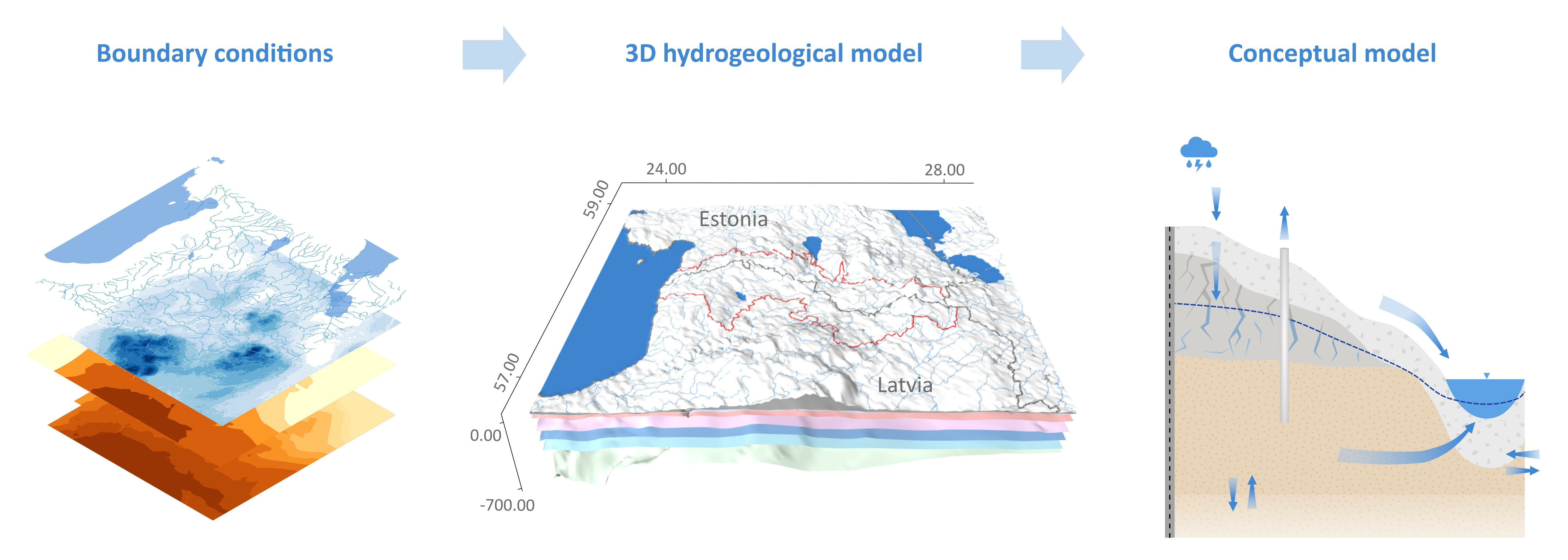
To further develop transboundary groundwater management activities between Estonia and Latvia, such as establishing a transboundary groundwater monitoring network or action programs for emergencies, a model for the transboundary aquifer system between Estonia and Latvia was developed. The study primary goals were to estimate transboundary groundwater flows, calculate the water budget, build a comprehensive conceptual understanding, and provide essential information to meet the aquifer management requirements set forth by the Water Convention and the EU Water Framework Directive. This model, developed using MODFLOW-6 software, integrates geological and hydrogeological factors and aims to enhance our understanding of this intricate system, facilitating more effective management and sustainable use of this vital shared resource.
2. Materials and Methods
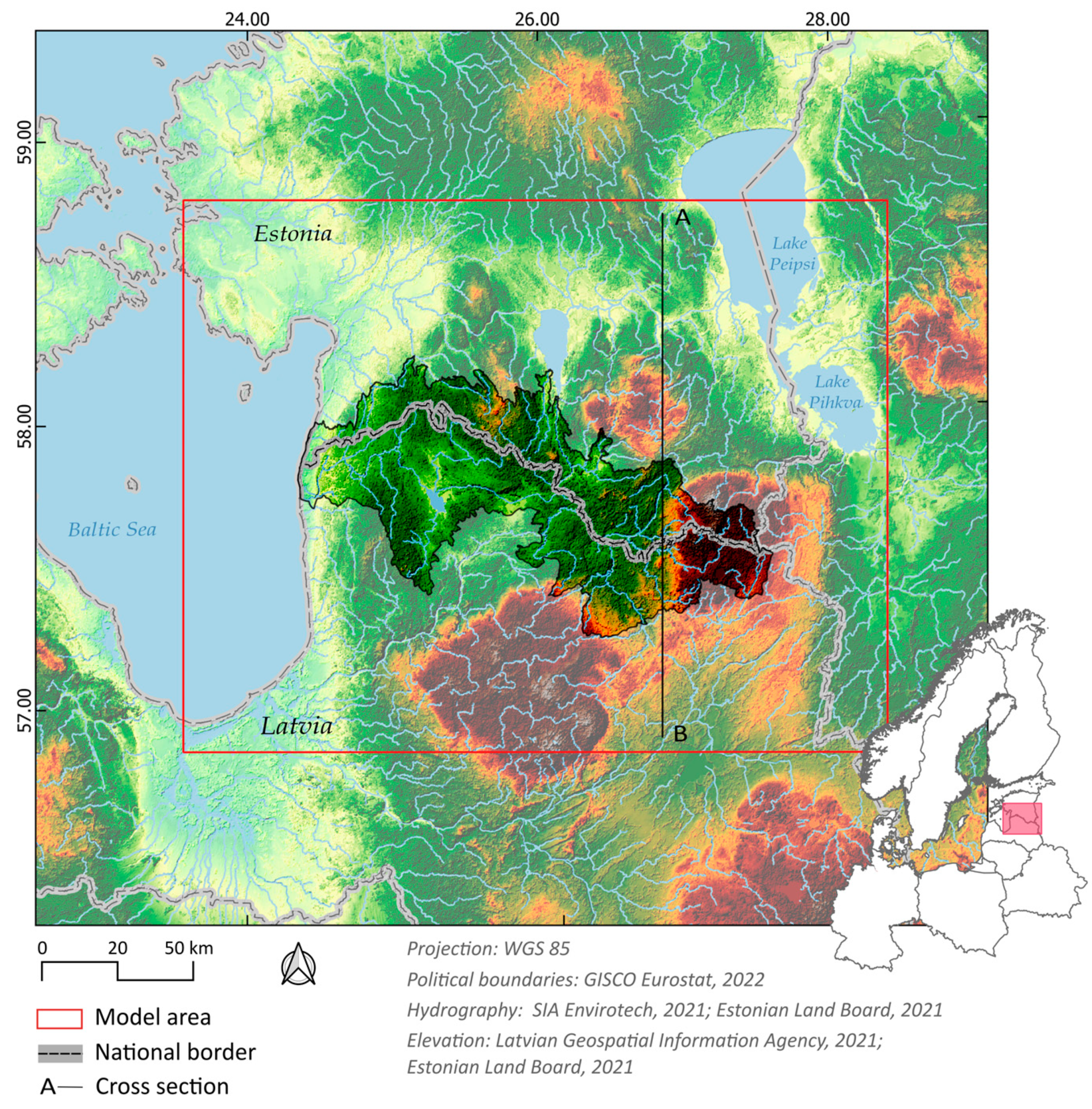
2.1. Description of Model Area
The study area is situated on the Baltic Sea coast in the North-East of Europe, covering approximately 45,000 km
2 (
Figure 1). The Baltic Sea borders it to the west, and Lake Peipsi and Lake Pihkva to the east. The topography is typically flat along the coast and hilly in the inland eastern part, with ground elevations ranging from 0 to 320 m above mean sea level (a.m.s.l). Most of the land is occupied by forests and semi-natural areas consisting of coniferous spruce, pine, white birch, ash, maple, and aspen, covering 58% of the study area. Agricultural lands, wetlands, and artificial surfaces follow after the forest and semi-natural areas [
34].
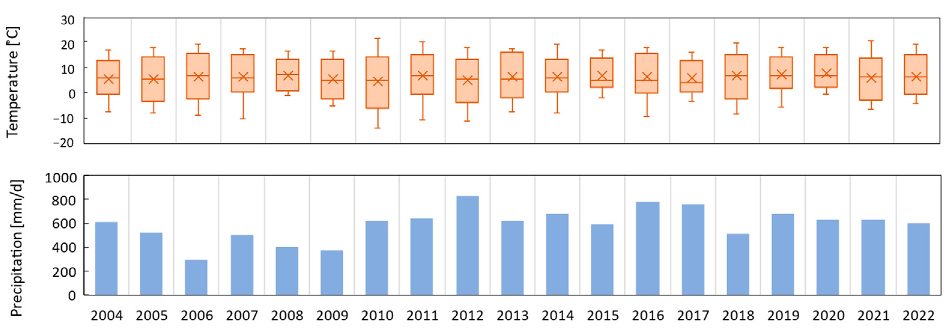
The climate in the region is moderately cool and humid [
35], with an average annual precipitation of 675 mm/yr and an average annual temperature of 6.3 °C (
Figure 2). The wettest months are June, August, and October, while the driest are March and April. The maximum average monthly temperature of 23.6 °C occurs in July, and the minimum average monthly temperature of −6.6 °C occurs in January [
36].
Evapotranspiration in temperate zone woodlands plays a significant role in the local hydrological cycle. On average, Baltic countries can exhibit evapotranspiration rates ranging from 400 to 600 mm per year. The rate of evapotranspiration in temperate woodlands is influenced by various factors, including temperature, humidity, solar radiation, and the type and density of vegetation [
37].
2.2. Hydrogeology
The model area contains sedimentary bedrock of Paleozoic (Cambrian, Ordovician, Silurian, and Devonian) and Proterozoic (Ediacaran) ages, consisting primarily of sandstone and limestone, that overlies Precambrian crystalline bedrock. The bedrock is predominantly flat-lying, with a southward regional dipping of approximately one to three meters per kilometer. Unconsolidated glacial deposits are superimposed over the bedrock formations throughout most of the model area. As the current study focuses on transboundary groundwater resources, only the upper units comprising Quaternary sediments, Devonian, and the upper Silurian formations are incorporated in the groundwater model.
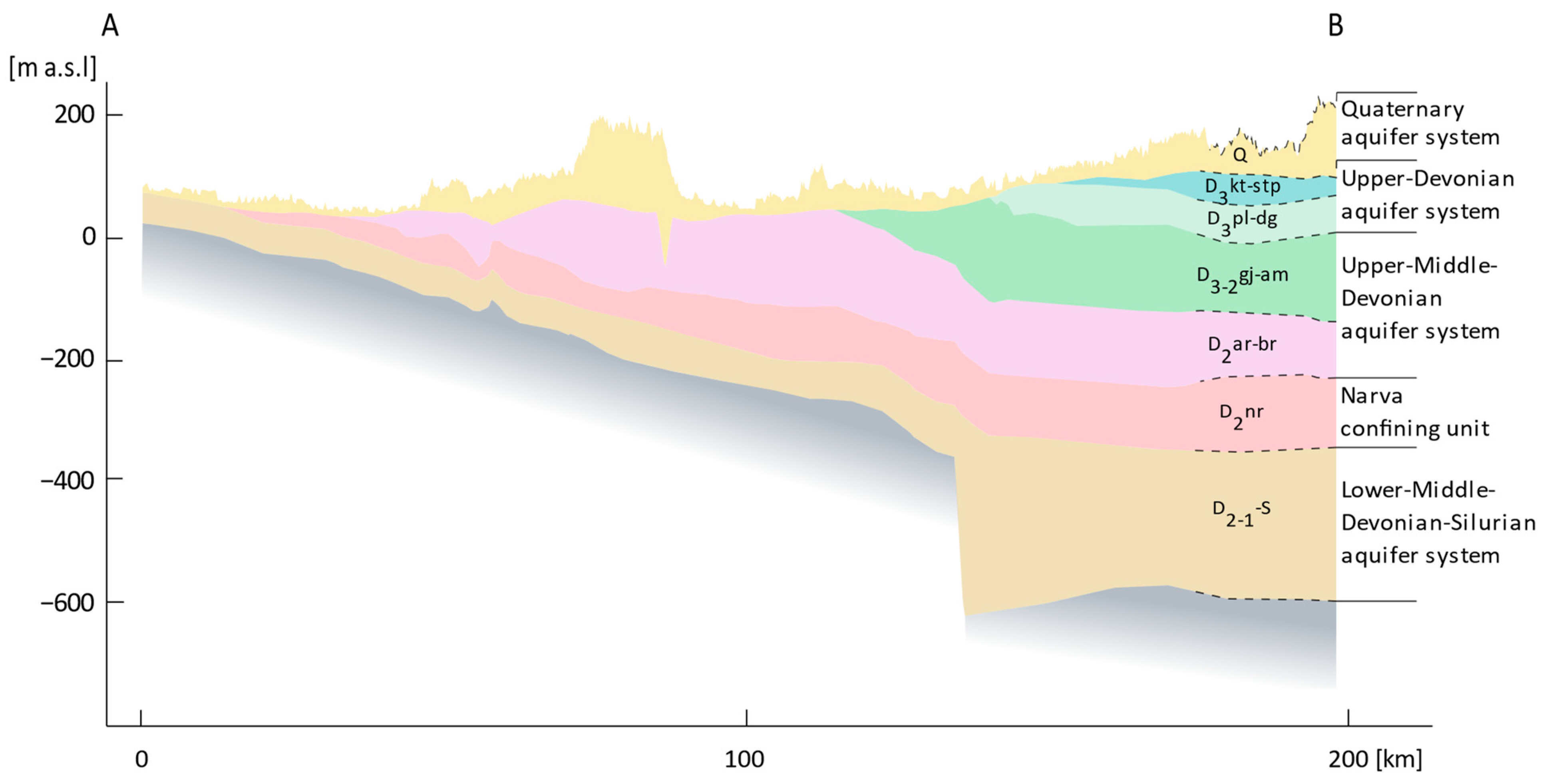
Thus, the modeled cross-section has four aquifer systems separated by confining units (
Table 1,
Figure 3 and
Figure 4):
Quaternary aquifer system (Q)
Upper-Devonian (Pļaviņas–Ogre) aquifer system (D3)
Upper-Middle-Devonian (Aruküla–Amata) aquifer system (D3-2)
Narva confining unit (D2nr)
Lower-Middle-Devonian aquifer system (D2-1)
The uppermost aquifer system is made up of Quaternary sediments, predominantly glacial till and glaciolacustrine sandy loam. The thickness of these deposits varies from less than 10 m to up to 100 m in buried valleys. The Upper-Devonian aquifer system, composed mainly of carbonate sediments, is found below the Quaternary sediments in the southeast, and it ranges in thickness from 17 m to 110 m. The Upper-Middle-Devonian aquifer system underlies the Upper-Devonian aquifer system in the southeast or is directly below the Quaternary sediments elsewhere, and it consists mostly of sandstones with clay and siltstone interlayers. The Narva confining unit separates the active water exchange zone from the slow water exchange zone and is 50–110 m thick. The Middle-Lower-Devonian–Silurian aquifer system lies below the Narva confining unit and is formed by Devonian and Silurian sedimentary formations, mainly sandstone, siltstone, and carbonates, which are heavily karstified in the upper part. Carbonates deeper than 100 m turn into the Silurian–Ordovician confining unit [
35].
2.3. Groundwater Model
To simulate the transient groundwater flow conditions, a 3D groundwater flow model was developed using MODFLOW-6 [
38], with the user interface of the open-source software ModelMuse version 4.3.0.0 [
39] developed by the U.S. Geological Survey. The finite-difference method was used to numerically solve the three-dimensional groundwater flow equation in a porous medium. The modular design of MODFLOW-6 enables the representation of groundwater-flow system processes, including recharge, flow, discharge, and interactions between aquifers and surface bodies. The model simulates transient conditions where inflows, outflows, and groundwater storage change over time. Recharge, discharge, and other groundwater-flow system processes are simulated based on yearly variations.
2.4. Water Balance and Change in Storage
The calibrated model quantifies all water budget components except for evapotranspiration. For the study area, the approximate average groundwater budget for the years 2010–2020 can be represented by Equation (1):
where R is recharge, S
in is groundwater coming in from storage, D is discharge, and S
out is groundwater going out to storage.
The groundwater system in the study area is recharged primarily through precipitation and seepage from streams. Water can be discharged from the system through seepage into streams, lakes, and seepage faces, pumping, evaporation from soil and transpiration by plants, and submarine seepage into the Baltic Sea. Detailed groundwater budgets are shown in the following Equation (2):
where R
ppt is recharge from precipitation, R
st is recharge from streams, R
lat is lateral inflow from neighboring areas, S
in is amount coming from storage, D
st is discharge to streams, D
sea is discharge to Baltic Sea, D
lake is discharge to lakes, D
et is discharge by evapotranspiration, D
pump is pumping amount from wells, D
lat is lateral outflow to neighboring areas, and S
out is amount going out to storage.
2.5. Model Grid and Layering
MODFLOW calculates hydraulic heads and flows within the model domain using data sets describing a groundwater-flow system hydrogeologic units, recharge, and discharge. To run the program, it is necessary to subdivide the groundwater-flow system into model cells vertically and horizontally. Each cell is assumed to have homogeneous hydraulic properties. The study area was horizontally discretized into square cells of 250 to 1000 m side length.
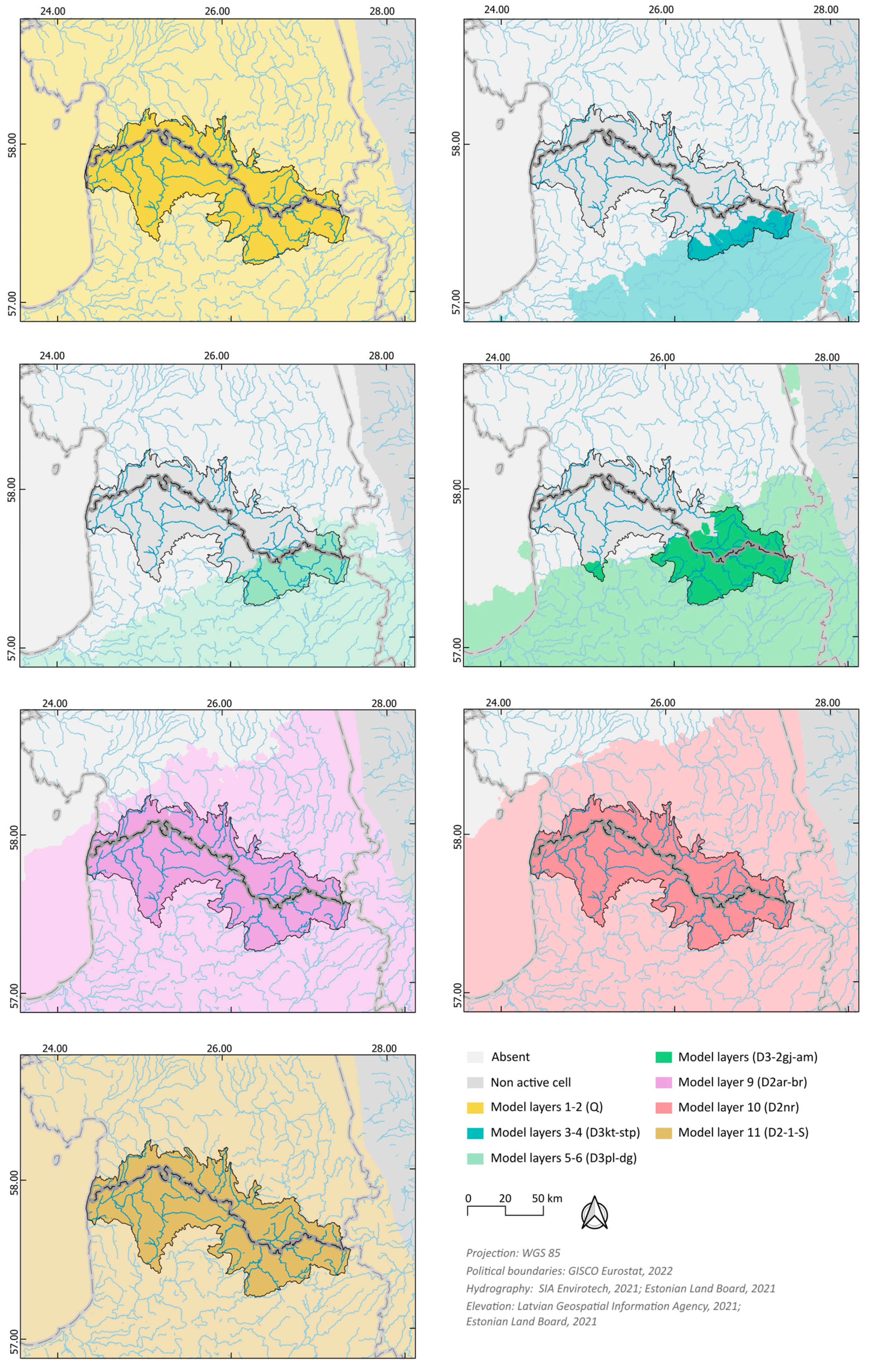
The model’s grid comprises eleven layers with varying thicknesses, with about 200,000 cells within each layer covering an area of 45,000 km
2. The model’s three-dimensional hydrogeologic framework and vertical layering were represented using the hydrogeologic units [
40,
41]. The thickness of hydrogeologic units in the study area may vary considerably over short distances due to buried valleys, and most units are not spatially contiguous throughout the model area.
Figure 3 illustrates the extent of active cells in each layer.
The geological surfaces of model layers vary spatially and correspond to the data published by Virbulis et al. [
41]. The Quaternary sediment unit is represented by layers 1 and 2 in the model (
Table 1,
Figure 3). The bedrock unit was divided into five aquifer and confining units—the Upper-Devonian aquifer system (layers 3–6), the Upper-Middle-Devonian aquifer system (layers 7–9), the Narva confining unit (layer 10), and the Lower-Middle-Devonian–Silurian aquifer system (layer 11). The model bottom (bottom of layer 11) represents the Silurian–Ordovician confining unit surface and is defined as a no-flow boundary.
2.6. Hydraulic Conductivity
Horizontal hydraulic conductivity was estimated for the hydrogeologic units using available field pumping test measurements [
42,
43]. Data were compiled and analyzed for 458 wells containing hydraulic conductivity, well-construction data, and lithologic descriptions. The median values of estimated hydraulic conductivity for the aquifers (
Table 2) are similar in magnitude to values compiled by Virbulis et al. [
41].
The vertical hydraulic conductivity values were initially set relative to the horizontal hydraulic conductivity during calibration using the anisotropy of 10 (Kv = Kh/10). The initial horizontal hydraulic conductivity values set to model layers varied among aquifer units, ranging from 0.8 m/d in the Upper-Middle-Devonian aquifer system to 100 m/d in the Upper-Devonian aquifer system. The Narva regional confining unit was assigned an initial horizontal hydraulic conductivity value of 2 × 10⁻⁹ m/d, while the Quaternary aquifer unit had an initial value of 10 m/d. In the Middle-Lower-Devonian–Silurian aquifer, the initial hydraulic conductivity was set at 5 m/d.
2.7. Storage Properties
Specific storage values were assigned to model layers to reflect changes in groundwater storage caused by changes in water levels in confined aquifers. According to Vallner and Porman [
35], specific storage in sandstones, limestones, and dolomites ranges from 1.0 × 10
–5 to 1.0 × 10
–3 m
–1. An initial specific storage value of 1.0 × 10
–6 m
–1 to all aquifer units and 1.0 × 10
–5 m
–1 to all confining units was assigned. These selections of specific storage values are based on the results of about 1000 time-drawdown pumping tests.
2.8. Boundary Conditions
No-flow boundary conditions exist on the model’s northern, eastern, southern, and western borders. Even though this boundary condition does not reflect the actual groundwater conditions at these locations, its effect on simulated conditions in the model nearfield is minimal because (1) there is a significant distance between the model boundaries and the model nearfield, and (2) other model boundary conditions limit its influence. A no-flow boundary also defines the bottom of the model (at the interface with the Silurian–Ordovician confining unit).
Recharge (RCH) is affected by the permeability of surface hydrogeologic units, relief, precipitation variations, and land cover characteristics in the study area. The initial recharge values were obtained from previous studies [
35] and applied to the model uppermost layer. In the study area, recharge values range from 0 m/d to 0.00081 m/d. Recharge values are constant through all stress periods.
A large part of the model represents the Baltic Sea, Lake Peipsi, Lake Pihkva, Lake Võrtsjärv, and Lake Burtnieki (
Figure 4). Each was assigned a Constant Head Boundary (CHB) (meters above mean sea level). The stages for four lakes were derived from a 10 m digital elevation model [
44,
45] using the minimum elevation within the lake area. Constant-head cells in the model are held constant through all stress periods.
To simulate the connectivity between the model domain and the wider Baltic Artesia Basin, a General Head Boundary (GHB) was assigned to cells along the southern extent of the model. The heads associated with this boundary were ascribed to the topographic surface elevation at each model cell. This involved model layer 11 of the LL-EE model. GHB conductance values were then calibrated to accommodate groundwater heads observed in wells near the boundary.
Streams are represented as River (RIV) boundary condition cells in the model. River locations were based on the stream network described in the databases [
46,
47]. River stages were calculated based on the minimum elevation [
44,
45] within each model cell that the river overlapped. The elevations were smoothed to eliminate rises in the direction.
Two meters from the river stage were subtracted to obtain the value of the river bottom. Each river cell initial riverbed hydraulic conductivity was set to 1 m/d.
A simulation of groundwater withdrawal from pumping wells was conducted using the WELL package. The daily pumping rates (cubic meters per day) were specified for each well for each stress period. Locations and pumping rates of wells were obtained from Estonian Environment Agency and Latvian Environment, Geology and Meteorology Centre databases [
42,
48].
3. Results and Discussion
3.1. Model Calibration
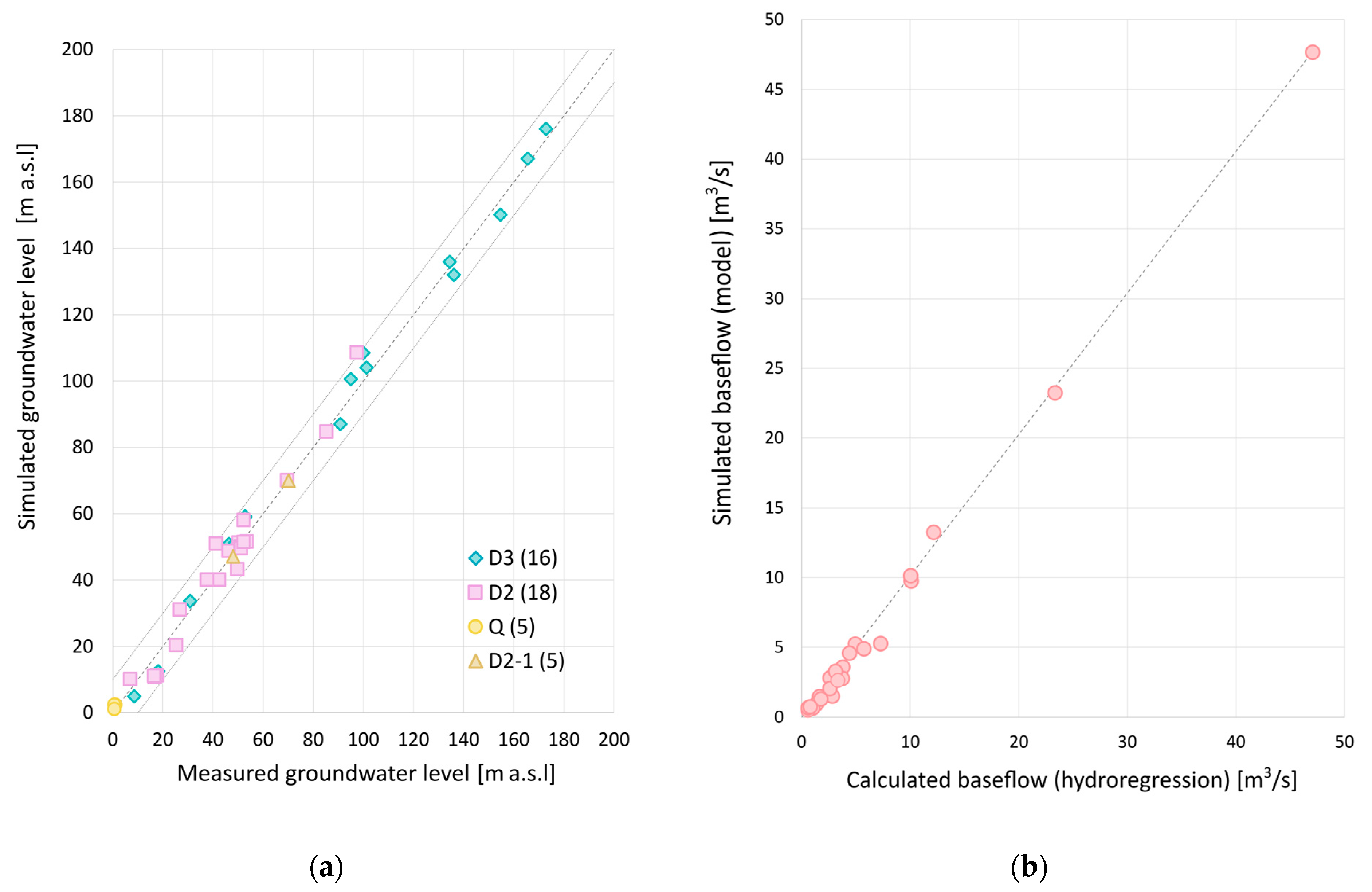
Water level and stream baseflow measurements were used to calibrate the groundwater flow model. A total of 44 water-level measurements from 40 wells were collected between January 2010 and December 2021. The Upper-Devonian aquifer system was represented by 16 wells, the Upper-Middle-Devonian aquifer system by 18 wells, and the Lower-Middle-Devonian–Silurian aquifer system by 5 wells. Additionally, streamflow was measured at 43 locations [
36,
49]. The hydrograph separation technique using the nonlinear reservoir algorithm [
50] was employed to estimate the baseflow component of the measured discharge.
The calibration results were evaluated by graphically and descriptively comparing the measured and simulated groundwater levels and streamflow values. This approach provided insights into the model fit and complemented the statistical measures. The model accuracy in replicating the flow system, particularly the regional direction and flow amounts, was assessed through this comparison.
The calibration results were further assessed using statistical parameters, including the mean, standard deviation, and root-mean-square error (RMSE). The RMSE values for water levels and stream baseflows were 4.5 m and 0.6 m
3/s, respectively, indicating a reasonable fit between the measured and simulated values. Regarding groundwater levels, the RMSE of 4.5 m accounted for approximately 2.6 percent of the average groundwater level range of 172 m (
Table 3). Similarly, the RMSE of 0.6 m
3/s for stream baseflows represented approximately 1.3 percent of the average range of 45.9 m
3/s. Importantly, the RMSE divided by the total range of values was less than 10%, indicating a satisfactory calibration level.
The comparison of the measured and simulated groundwater-level data revealed that the simulated values aligned well with the measured values along the line of equal measured and simulated values. However, there was a tendency to underestimate groundwater level altitudes within the range of 30–60 m (
Figure 5a).
The comparison of the measured and simulated groundwater discharge to streams (baseflow) demonstrated a good agreement between the two, as indicated by the line representing equal measured and simulated values (
Figure 5b).
In the context of our calibrated hydrogeological model, we have refined the horizontal hydraulic conductivities for various aquifer units within the study area. These adjustments reflect a more precise characterization of groundwater flow characteristics. Specifically, the Quaternary aquifer conductivity values now range from 0.2 m/d at the minimum and to 5 m/d at the maximum. The Upper-Devonian aquifer exhibits a refined conductivity range, with values spanning from 0.3 m/d as the minimum to 50 m/d as the maximum. The Upper-Middle-Devonian aquifer calibrated conductivity values fall within the range of 0.8 m/d at the minimum and to 6 m/d at the maximum.
In contrast, the Narva confining unit, acting as a regional aquitard, exhibits a notable disparity in hydraulic conductivity, ranging from 1.4 m/d at the maximum end to an extremely low 1.00 × 10⁻⁹ m/d at the minimum, reflecting its reduced permeability. Lastly, the Middle-Lower-Devonian–Silurian aquifer maintains relatively consistent hydraulic conductivity value– 2 m/d. These adjustments, based on calibration results, align the model more closely with observed groundwater behavior, enhancing its reliability for groundwater management and environmental assessments within the study area.
3.2. Groundwater Level and Water Balance
Based on the calibrated model, all water budget components could be quantified except for evapotranspiration. The simulated groundwater budgets revealed substantial recharge from precipitation and inflow from adjacent areas in the model area. The water balance components are shown in
Figure 6 and
Figure 7 and listed in
Table 4.
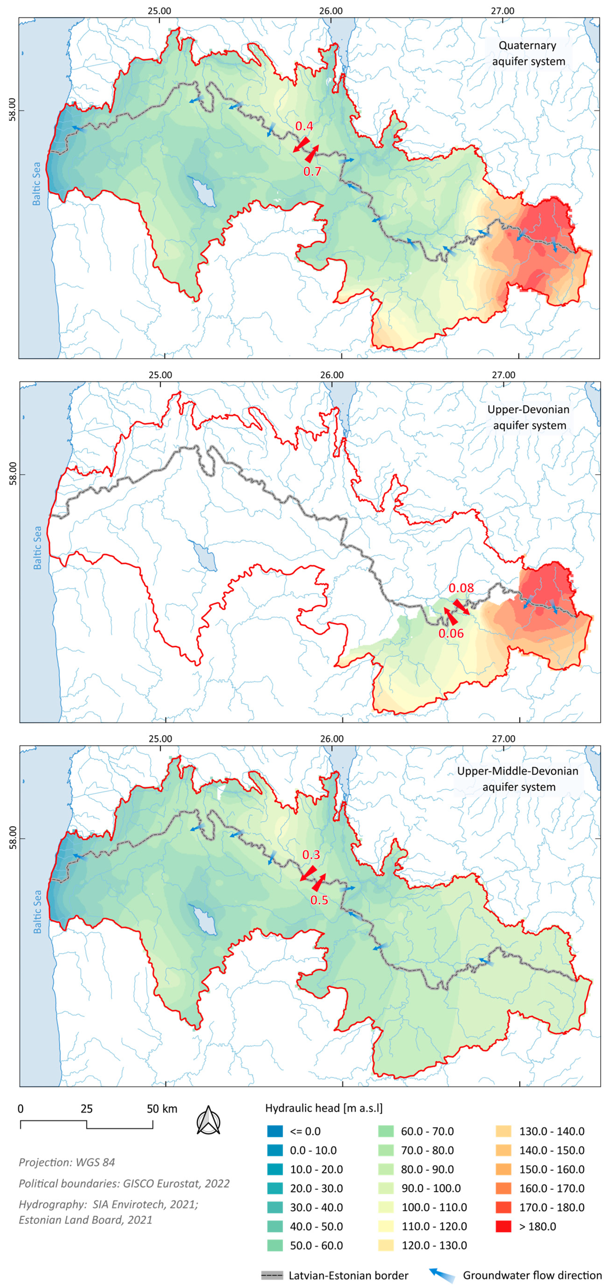
The simulated groundwater budget for the Quaternary aquifer indicates that this aquifer typically receives recharge from precipitation and groundwater inflow from the underlying Upper-Devonian and Upper-Middle-Devonian aquifer (
Table 4). Groundwater discharge to streams is the largest component of aquifer discharge. Groundwater withdrawal and groundwater outflow to the Baltic Sea and underlying Upper-Devonian and Upper-Middle-Devonian aquifer accounts for a smaller total discharge compared to discharge to streams from the aquifer.
The simulated groundwater budget for the Upper-Devonian aquifer indicates that it primarily receives recharge inflow from the overlying Quaternary aquifer and from adjacent areas (
Table 4). Smaller component of simulated recharge for the Upper-Devonian aquifer is groundwater inflow from the underlying Upper-Middle-Devonian hydrogeologic unit. The primary discharge component for the Upper-Devonian aquifer is groundwater outflow to the overlying Quaternary hydrogeologic unit. The remaining discharge components from the Upper-Devonian aquifer are groundwater withdrawals, discharge to streams, the Baltic Sea, groundwater outflow to the adjacent areas, and the underlying Upper-Middle-Devonian aquifer system.
Simulated recharge to the Upper-Middle-Devonian aquifer is primarily groundwater inflow from the overlying Upper-Devonian aquifer (
Table 4). Minor simulated recharge components are groundwater inflow from adjacent areas and the underlying Narva confining system. Groundwater inflow from the adjacent areas and inflow from the underlying Narva hydrogeologic unit accounts for a much smaller component of overall recharge compared to groundwater inflow from the overlying Quaternary hydrological unit and Upper-Devonian aquifer to the Upper-Middle-Devonian aquifer. Primary discharge components for the Upper-Devonian aquifer are discharged to streams and groundwater outflow to the overlying Upper-Devonian aquifer. Minor discharge components are groundwater withdrawals and groundwater outflow to the Baltic Sea. Groundwater flow in the Upper-Middle-Devonian aquifer is much more regionalized than the overlying aquifers; however, local discharge is to major streams (
Figure 6).
Despite the unequal distribution of cross-border groundwater flows along the Estonian–Latvian border, the amounts of groundwater moving across the border are comparable. In the Quaternary aquifer system, groundwater flows occurred in both directions (
Figure 6). The total flow in the Quaternary aquifer from Estonia to Latvia is 38,928 m
3/d and from Latvia to Estonia 71,639 m
3/d, based on which the total net flow is 32,711 m
3/d. The Upper-Devonian aquifer is predominantly present in the eastern part of the pilot area, and groundwater flow patterns vary along the border. The total flow in the Upper-Devonian aquifer from Estonia to Latvia is 8398 m
3/d, and from Latvia to Estonia is 5777 m
3/d, and the total net flow is 2621 m
3/d. The Upper-Middle-Devonian aquifer system represents most of the transboundary groundwater flow across the Estonian–Latvian pilot area, with a total flow from Latvia to Estonia of 54,522 m
3/d, a total flow from Estonia to Latvia of 31,141 m
3/d, and a net flow of 23,381 m
3/d (
Figure 6).
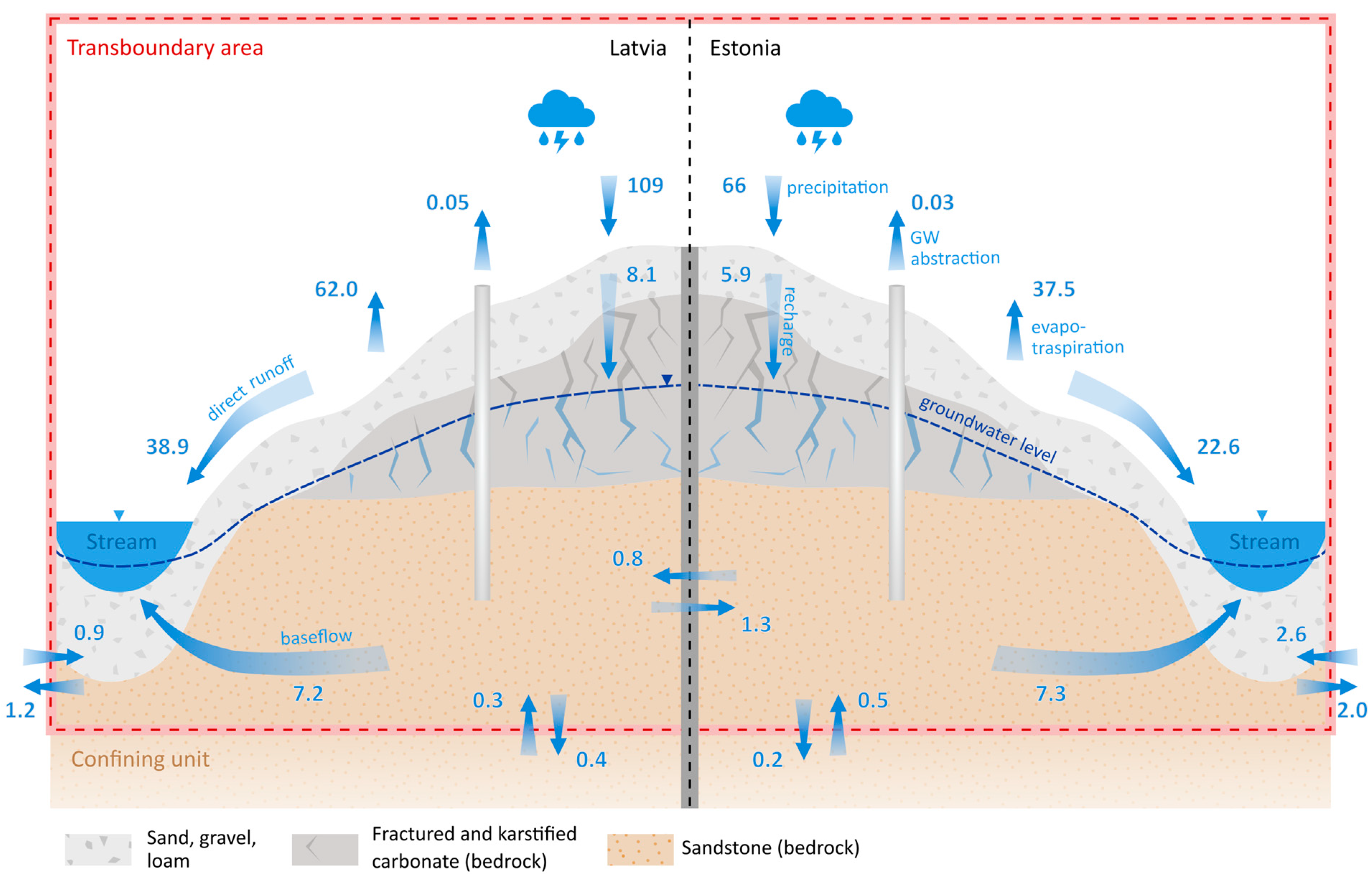
Figure 7 illustrates the conceptual model of the water balance of all three aquifers and groundwater flow across borders. The study area water balance analysis revealed important findings regarding precipitation distribution, infiltration, groundwater flow, and the dynamics of deeper aquifers. The distribution of precipitation showed that approximately 34–36% of the total precipitation directly contributes to surface water bodies, such as rivers, lakes, and streams. This indicates a significant portion of water immediately becomes part of the surface water resources.
In terms of infiltration, only 7–9% of the precipitation infiltrates the subsurface, replenishing the groundwater reserves. This highlights the limited amount of water that seeps into the subsurface and contributes to groundwater recharge. Approximately 7–11% of the total water balance moves through groundwater and returns to surface water bodies. This emphasizes the significance of groundwater as a contributor to the overall water flow in the study area.
The study also examined the direction of groundwater recharge and flow. The results showed that only 3–5% of the total recharge infiltrates deeper aquifers, while the remaining groundwater either returns to surface water bodies or flows into aquifers outside the study area. This suggests that a significant amount of groundwater does not contribute to the recharge of the cross-border area, likely due to the prevailing flow patterns and geological characteristics. The model calculations indicated that 89–124% of the total water balance flows from groundwater to surface water bodies as baseflow. This range suggests that groundwater plays a crucial role in sustaining the baseflow in surface water bodies, compensating for the deficit in groundwater recharge from outside the study area.
Based on the conceptual model, the active water exchange zone within the study area was found to extend to a depth of approximately 200 m, up to the Narva confining unit. This zone is identified as the most sensitive to pollution and susceptible to climate change due to the extensive water exchange and interactions with surface water bodies.
4. Conclusions
This study aimed to calibrate a groundwater flow model using water level and stream baseflow measurements in the North-East European coastal region. The comparison between measured and simulated data, both graphically and statistically, demonstrated a satisfactory fit of the model. The calibrated model provided valuable insights into the flow dynamics and water budget components, including recharge, discharge, and transboundary groundwater flow patterns. The results highlighted the significance of the Quaternary, Upper-Devonian, and Upper-Middle-Devonian aquifer systems in the study area, with varying groundwater flow rates and directions across the Estonian–Latvian border area.
The findings of the modeling study indicate a strong hydrological connection between groundwater and surface water within the initial 200 m of a cross-section. This has significant implications for water management in the area. Notably, approximately 90% of infiltrated groundwater contributes to the baseflow of local rivers, while only a small proportion recharges deeper layers within the cross-section.
The observed water usage in the area suggests that the area can be considered in a state of natural conditions, as the actual water consumption is orders of magnitude lower than the recharged groundwater. In such natural conditions, the transboundary flow is considerably smaller than groundwater flow from recharge areas to nearby surface water bodies. Consequently, future activities and plans must carefully consider the potential effects of water usage on both cross-border flow and the baseflow of local surface water bodies, namely the groundwater-associated aquatic ecosystems.
The findings have implications for sustainable groundwater management, particularly in terms of water resource planning and allocation. The calibrated model and its outputs can support decision-making processes and facilitate informed strategies for protecting and efficiently utilizing groundwater resources and groundwater-dependent ecosystems in this region.


