Composition and Reactivity of Volatile Organic Compounds and the Implications for Ozone Formation in the North China Plain

Abstract

Enhanced ozone (O₃) pollution has emerged as a pressing environmental concern in China, particularly for densely populated megacities and major city clusters. However, volatile organic compounds (VOCs), the key precursors to O₃ formation, have not been routinely measured. In this study, we characterize the spatial and temporal patterns of VOCs and examine the role of VOCs in O₃ production in five cities (Dongying (DY), Rizhao (RZ), Yantai (YT), Weihai (WH), and Jinan (JN)) in the North China Plain (NCP) for two sampling periods (June and December) in 2021 through continuous field observations. Among various VOC categories, alkanes accounted for the largest proportion of VOCs in the cities. For VOCs, chemical reactivities, aromatic hydrocarbons, and alkenes were dominant contributors to O₃ formation potential (OFP). Unlike inland regions, the contribution to OFP from OVOCs increased greatly at high O₃ concentrations in coastal regions (especially YT). Model simulations during the O₃ episode show that the net O₃ production rates were 27.87, 10.24, and 10.37 ppbv/h in DY, RZ, and JN. The pathway of HO₂ + NO contributed the most to O₃ production in JN and RZ, while RO₂ + NO was the largest contributor to O₃ production in DY. The relative incremental reactivity (RIR) revealed that O₃ formation in DY was the transitional regime, while it was markedly the VOC-limited regime in JN and RZ. The O₃ production response is influenced by NOx concentration and has a clear daily variation pattern (the sensitivity is greater from 15:00 to 17:00). The most efficiencies in O₃ reduction could be achieved by reducing NOx when the NOx concentration is low (less than 20 ppbv in this study). This study reveals the importance of ambient VOCs in O₃ production over the NCP and demonstrates that a better grasp of VOC sources and profiles is critical for in-depth O₃ regulation in the NCP.

1. Introduction

Tropospheric ozone (O₃) is a secondary pollutant that forms through the photooxidation of precursors in the presence of sunlight. Elevated O₃ levels greatly contribute to the degradation of regional air quality [1]. Exposure to high O₃ levels has been linked to detrimental health effects including cardiovascular diseases, respiratory infections, and neurodevelopment disruptions [2,3]. Over the past decade, major city clusters in China have been suffering from elevated O₃ pollution, with high rates of morbidity and mortality related to O₃ exposure. In addition to adverse health outcomes, high O₃ levels are detrimental to plants and crops through reducing the carbon sequestration of vegetation [4,5].

The regulation of O₃ pollution is challenging due to the non-linear relationship between O₃ and its precursors (including volatile organic compounds (VOCs) and nitrogen oxides (NOx)) [6]. The chemical composition and sources of VOCs are complex and varied [7]. Generally, VOCs were divided into six types, namely alkanes, alkenes, alkynes, aromatic hydrocarbons, halogenated hydrocarbons, and oxygenated VOCs (OVOCs). The spatial distribution of VOCs throughout China has been extensively investigated in previous studies [8,9]. Alkanes have been widely identified as the dominant VOCs in northern China [10], and OVOCs predominate in the hilly regions of southeast China [11]. Furthermore, it was reported that higher aromatic hydrocarbon levels were depicted in Shanghai due to substantial solvent usage [12]. Despite the abovementioned extensive studies on the identification of dominant VOC species and source apportionment of VOCs, the sources of ambient VOCs in northern China remain poorly understood.

Northern China has been identified as a highly polluted area affected by frequent O₃ episodes [13]. In particular, densely populated cities in the Shandong Peninsula have suffered high levels of O₃ exposure and act as receptors of regional O₃ air mass under synoptic patterns. However, less attention has been paid to this region and limited prior work is insufficient for elucidating O₃ formation over the Shandong Peninsula. Therefore, it is critical to investigate the spatial and temporal pattern of ambient VOCs across this region and examine the chemical reactivity of VOCs among cities in the Shandong Peninsula. In 2021, field measurements of VOCs were conducted at five cities within the Shandong Peninsula, including Jinan (JN), Dongying (DY), Rizhao (RZ), Yantai (YT), and Weihai (WH). DY, RZ, YT, and WH are coastal cities located in the eastern Shandong Peninsula, and DY has urban O₃ precursor emissions in close proximity to industrial sectors (oil field extraction) [14]. As the capital city of Shandong Province, Jinan (JN) is a typical city which experienced severe O₃ pollution under the transport pathway in northern China [15]. The detailed measurements for these cities are expected to shape a clear map of VOC composition and shed further light on the development of effective O₃ regulation policies.

In this study, we combine field measurements and box modeling to characterize the sources of VOCs and identify the influence of VOC emissions on O₃ production in the Shandong Peninsula. The composition and temporal pattern of ambient VOCs was sampled and analyzed in five cities in the Shandong Peninsula for the periods of June and December 2021. The chemical reactivity of VOCs was calculated by means of the maximum incremental reactivity method (MIR). Furthermore, box modeling was performed using the MCM model for investigating O₃ production pathways in coastal and inland cities in summer, and key VOC species affecting O₃ production were identified. Sensitivity experiments configured with varied ratios of VOCs and NOx reduction were conducted to provide a theoretical basis for the development of O₃ mitigation strategies in the Shandong Peninsula.

2. Materials and Methods

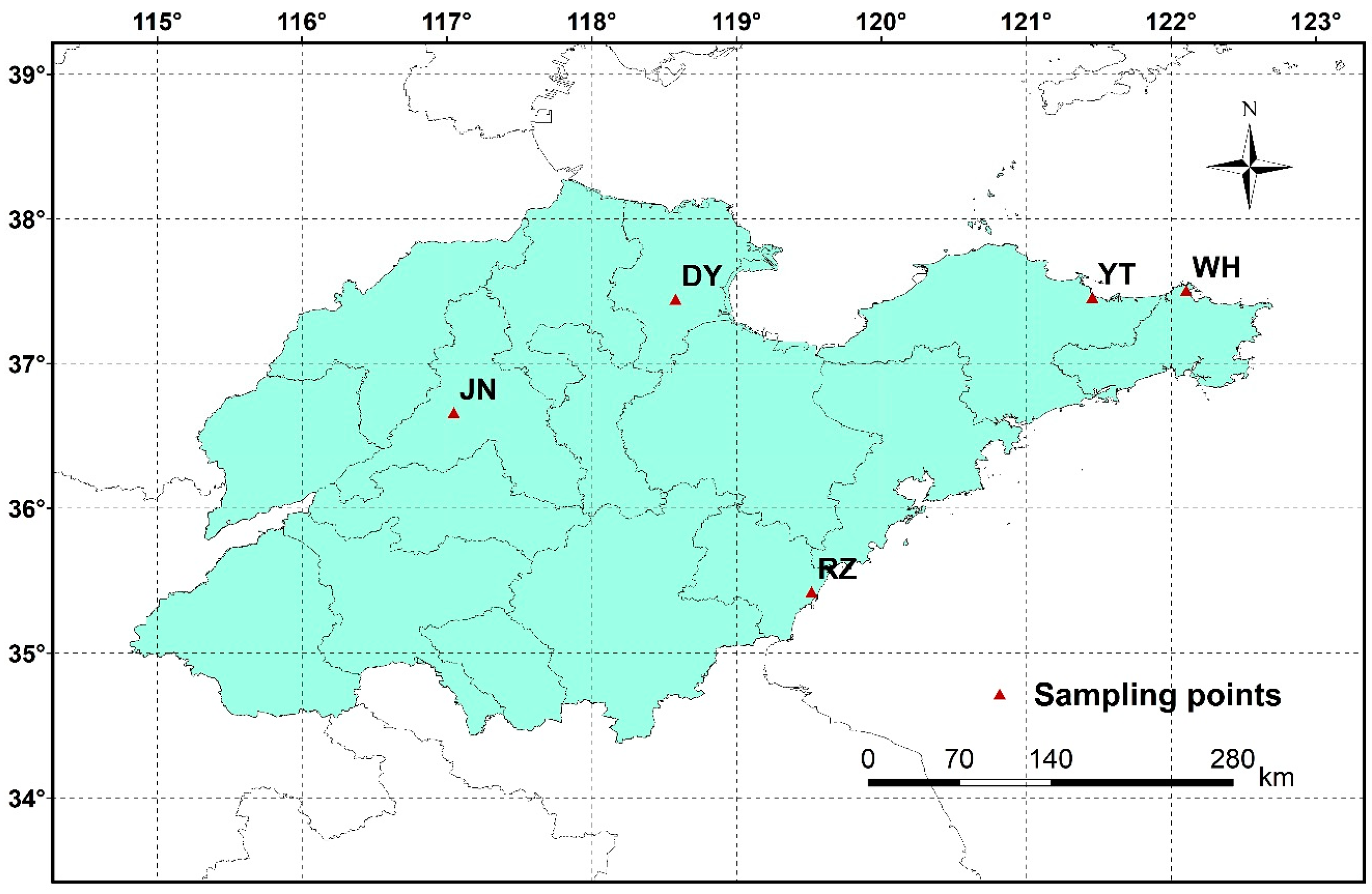
2.1. Data Sampling and Quality Assurance/Quality Control

In this study, ambient measurements were conducted at five typical monitoring sites in Shandong Province (locations shown in Figure 1), and the main sources of pollution around the monitoring sites were shown in Figure S1. The monitoring sites included the coastal cities YT, WH, RZ, and DY, and the inland city JN. DY (118.5812° E, 37.4473° N) is located near an oil field exploitation area, with a single source of pollution; there are major petrochemical industry emission sources in the northeast. JN (117.0494° E, 36.6627° N) is located in the center of the city, and is surrounded by a large number of gas stations and construction sites. Sites YT (121.458611° E, 37.46° N), WH (122.1067° E, 37.5069° N), and RZ (119.5192° E, 35.4242° N) are located in the offshore area of the city, where air quality is relatively good.

The VOC data were obtained from the GC955-611 (Hangzhou Juguang Technology Co., Ltd., Hangzhou, China) high boiling point O₃ precursor analyzer online monitoring equipment, which mainly consists of a photo ionization detector and flame ionization detector, a pre-concentration tube, a pre-separation column, an analytical column, a ten-pass valve, and a built-in computer PC, etc. The instrument is loaded with high-purity nitrogen gas and injected at 50 °C without a shunt, and the monitored VOCs included 96 VOC monomers, including 29 alkanes, 11 alkenes, 16 aromatic hydrocarbons, 1 alkyne, 30 halogenated hydrocarbons, and 9 OVOCs. The specific component names are shown in Table S1. The sampling time resolution was 1 h, and 3498 valid samples were obtained over 24 h of continuous monitoring. The online monitor was calibrated every 10 d during the sampling period. The meteorological data were collected simultaneously from the ambient air automatic online monitoring sites with a time resolution of 1 h.

The quality assurance and quality control (QA/QC) of the monitored data is carried out according to the guideline entitled “Specifications and Test Procedures for Ambient Air Quality Continuous Monitoring System with Gas Chromatography for Volatile Organic Compounds” (HJ 1010-2018). The method detection limits (MDLs) of components are 0.01 ppb. The concentration of the blank sample is less than 0.01 ppb. The standard gas was prepared with a volume fraction gradient of 0.5 ppb, 2 ppb, 4 ppb, 6 ppb, 8 ppb, and 10 ppb, and the correlation coefficient of the calibration result should be more than 0.98.

2.2. Ozone Formation Potential

The OFP indicates the potential contribution of individual VOC species to O₃ production, which is an indicator parameter that integrates the reactivity of VOC species to O₃ formation. It can be calculated based on the MIR method [16], and the MIR of VOC species was updated by a previous study [17]. In this study, the OFP of individual VOC species was calculated as follows:

$$C_j^{\mathrm{M}\mathrm{I}\mathrm{R}}=\mathrm{M}\mathrm{I}\mathrm{R}\times C_j,$$

(1)

$${\mathrm{O}\mathrm{F}\mathrm{P}}_{\mathrm{M}\mathrm{I}\mathrm{R}}=\sum C_j^{\mathrm{M}\mathrm{I}\mathrm{R}},$$

(2)

where $C_j^{\mathrm{M}\mathrm{I}\mathrm{R}}$ denotes the maximum O₃ concentration that can be produced by VOC species j, MIR denotes the maximum incremental reactivity of VOC species j, Cj denotes the measured concentration of VOC species j (μg/m³), and OFP_MIR denotes the sum of the maximum O₃ concentration that can be produced by VOC species.

2.3. Weather Research and Forecasting Model

In this study, the Weather Research and Forecasting (WRF) v3.9.1 model was used to simulate meteorological fields from 6 to 22 June 2021 over the NCP region. The initial and boundary conditions of the WRF model were obtained from reanalysis datasets of the National Center for Atmospheric Research (NCAR) with a temporal resolution of 6 h and a spatial resolution of 1° × 1° (https://rda.ucar.edu/datasets/ds083.2/, accessed on 20 October 2022). The vertical resolution of the WRF model was 34 layers. In order to reduce the ambiguity around the initial conditions, the first three days were regarded as the spin-up, which was not included in the analysis. The more detailed options relating to WRF are detailed in Wang et al. [18].

2.4. Observation-Based Model

The Master Chemical Mechanism (MCM, v3.3, http://mcm.leeds.ac.uk/MCM/, accessed on 1 March 2023) model is one of the most important models for investigating atmospheric chemical mechanisms, including 17,000 atmospheric chemical reaction processes of 143 VOCs. Moreover, it is widely used for atmospheric O₃ production mechanisms and VOC sensitive species screening [19,20,21].

The in situ O₃ production and loss rates were calculated as follows [22,23]: In the troposphere, O₃ production is formed by the reactions of HO₂ + NO and RO₂ + NO. In contrast, O₃ destruction reactions include O₃ photolysis and reactions with VOCs, OH, HO₂, and the reaction of OH + NO₂, RO₂ + NO₂, and VOCs + NO₃. The net O₃ production is defined as the difference between P(O₃) and L(O₃).

$$\mathrm{P}\left({\mathrm{O}}_3\right)=k_1\left[{\mathrm{H}\mathrm{O}}_2·\right]\left[\mathrm{N}\mathrm{O}\right]+\sum k_2\left[{\mathrm{R}\mathrm{O}}_2·\right]\left[\mathrm{N}\mathrm{O}\right],$$

(3)

$$\begin{gathered} \mathrm{L}\left({\mathrm{O}}_3\right)=k_3\left[{\mathrm{O}}^1\left(\mathrm{D}\right)\right]\left[·\mathrm{O}\mathrm{H}\right]+k_4\left[·\mathrm{O}\mathrm{H}\right]\left[{\mathrm{O}}_3\right]+k_5\left[{\mathrm{H}\mathrm{O}}_2·\right]\left[{\mathrm{O}}_3\right]+k_6\left[·\mathrm{O}\mathrm{H}\right]\left[{\mathrm{N}\mathrm{O}}_2\right]+ \\ {k}_7\left[{\mathrm{R}\mathrm{O}}_2·\right]\left[{\mathrm{N}\mathrm{O}}_2\right]+2\sum \left(k_{8i}\left[{\mathrm{V}\mathrm{O}\mathrm{C}}_i\right]\left[{\mathrm{N}\mathrm{O}}_3·\right]\right)+\sum \left(k_{9i}\left[{\mathrm{V}\mathrm{O}\mathrm{C}}_i\right]\left[{\mathrm{O}}_3\right]\right), \end{gathered}$$

(4)

$$\mathrm{N}\mathrm{E}\mathrm{T}\mathrm{P}\left({\mathrm{O}}_3\right)=\mathrm{P}\left({\mathrm{O}}_3\right)-\mathrm{L}\left({\mathrm{O}}_3\right)$$

(5)

where P(O₃) denotes the O₃ production rate (ppbv/h), L(O₃) represents the O₃ destruction rate (ppbv/h), and k denotes the photochemical reaction rate of the reaction.

The specific model settings of MCM in this study are as follows: During the model simulation, the input data included O₃, VOCs, NOx, and meteorological parameters (Relative humidity, atmospheric pressure, and temperature) with a resolution of 1 h. A special case of a day with high O₃ concentration and complete observation data of the corresponding precursors was selected for model calculation. In this study, the O₃ production and destruction cycle of the high O₃ day was simulated. The model started at 00:00 BST. To ensure the stability of the whole simulation, it was necessary to run it 5 days in advance to obtain the stable concentrations of other atmospheric active species without observations.

In this study, the MCM model simulations were conducted to calculate the daily RIR during O₃ episodes to diagnose O₃ production mechanism. In addition, sensitivity experiments with emission reductions were conducted to probe the RIR changes in response to the reduction of the O₃ precursor. The calculation equation is as follows [19]:

$$\mathrm{R}\mathrm{I}\mathrm{R}\left(\mathrm{X}\right)=\frac{\Delta \mathrm{P}\left({\mathrm{O}}_3\right)\left(\mathrm{X}\right)/\mathrm{P}\left({\mathrm{O}}_3\right)\left(\mathrm{X}\right)}{\Delta \left(\mathrm{X}\right)/\mathrm{X}},$$

(6)

where ΔP(O₃) denotes O₃ production rate variations and ∆(X) denotes the concentration variations of precursor X (VOCs, NO, NO₂).

3. Results

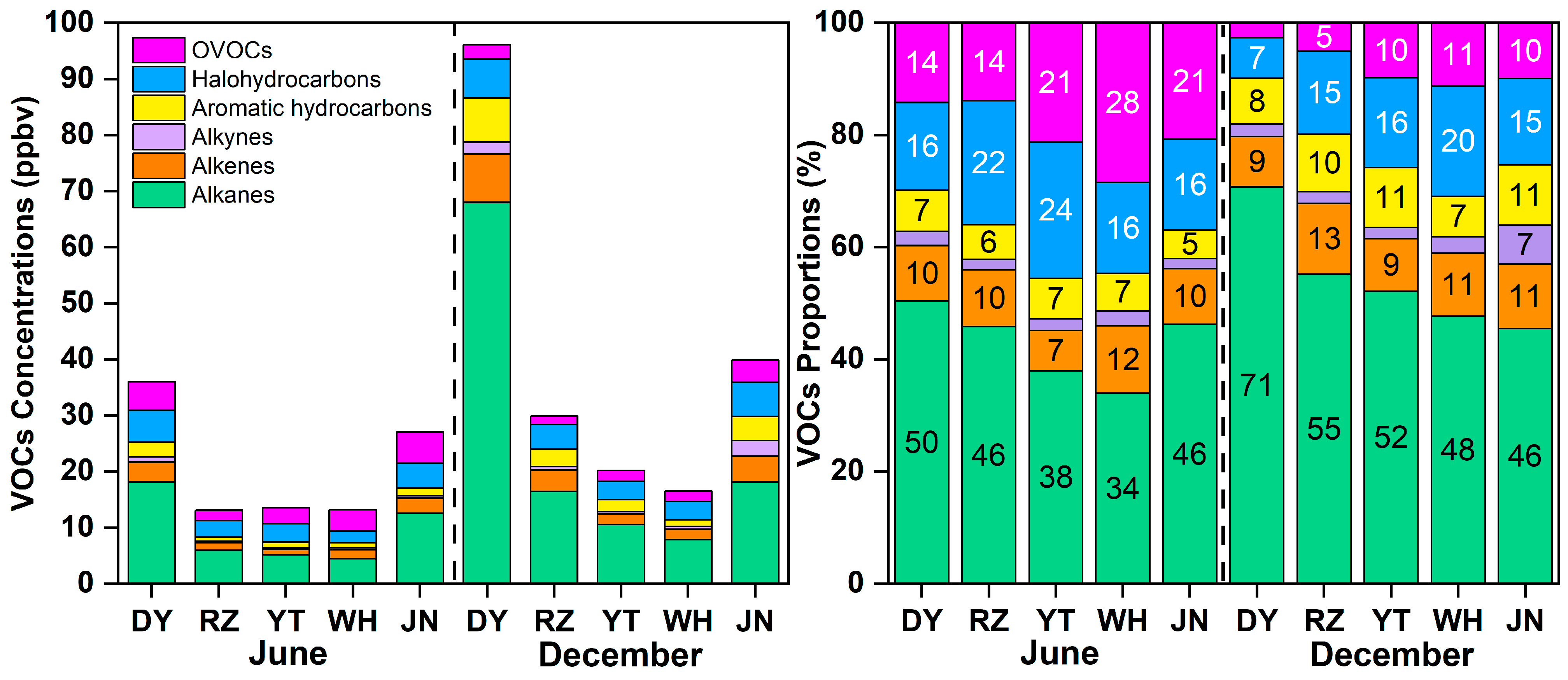
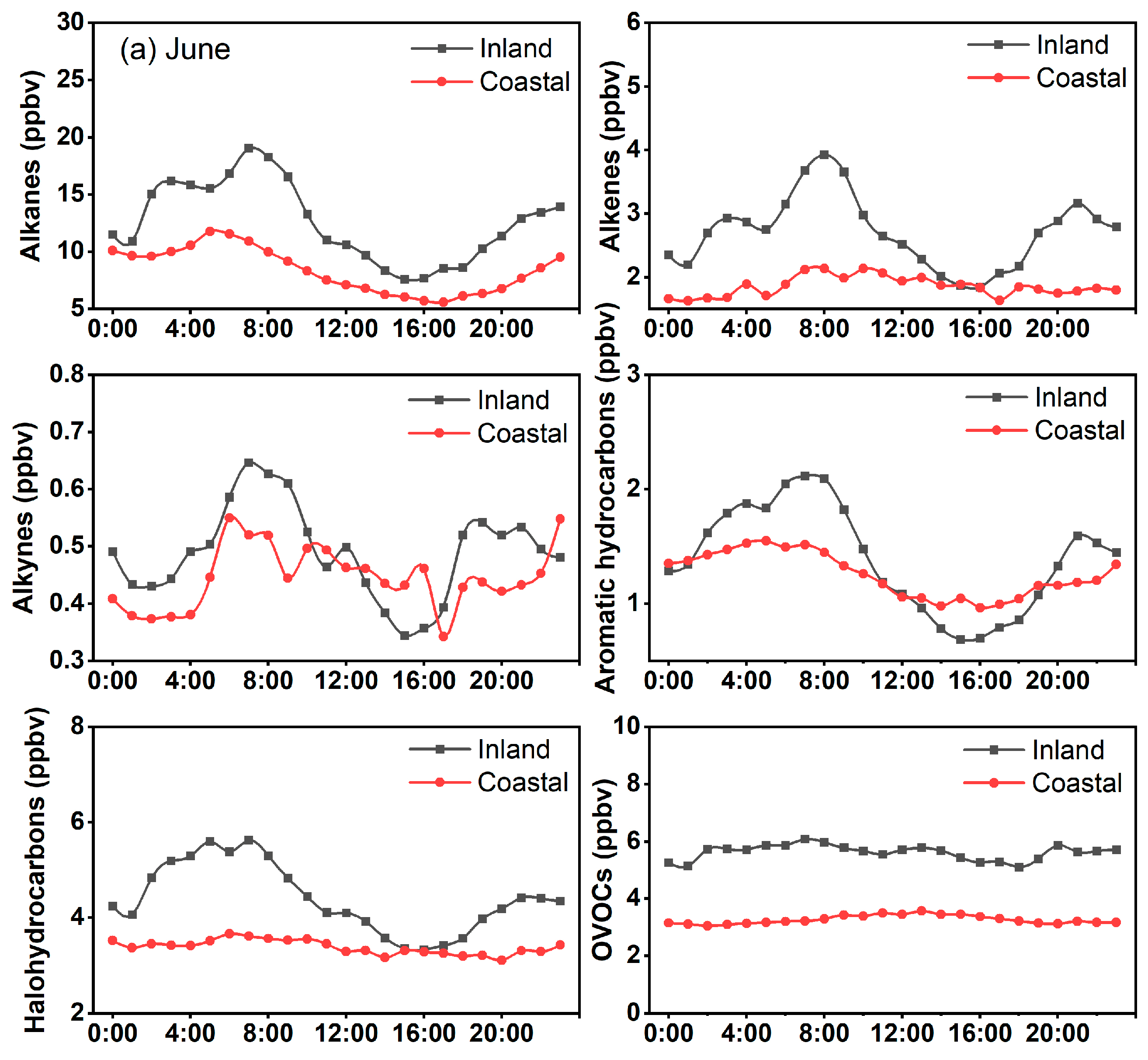
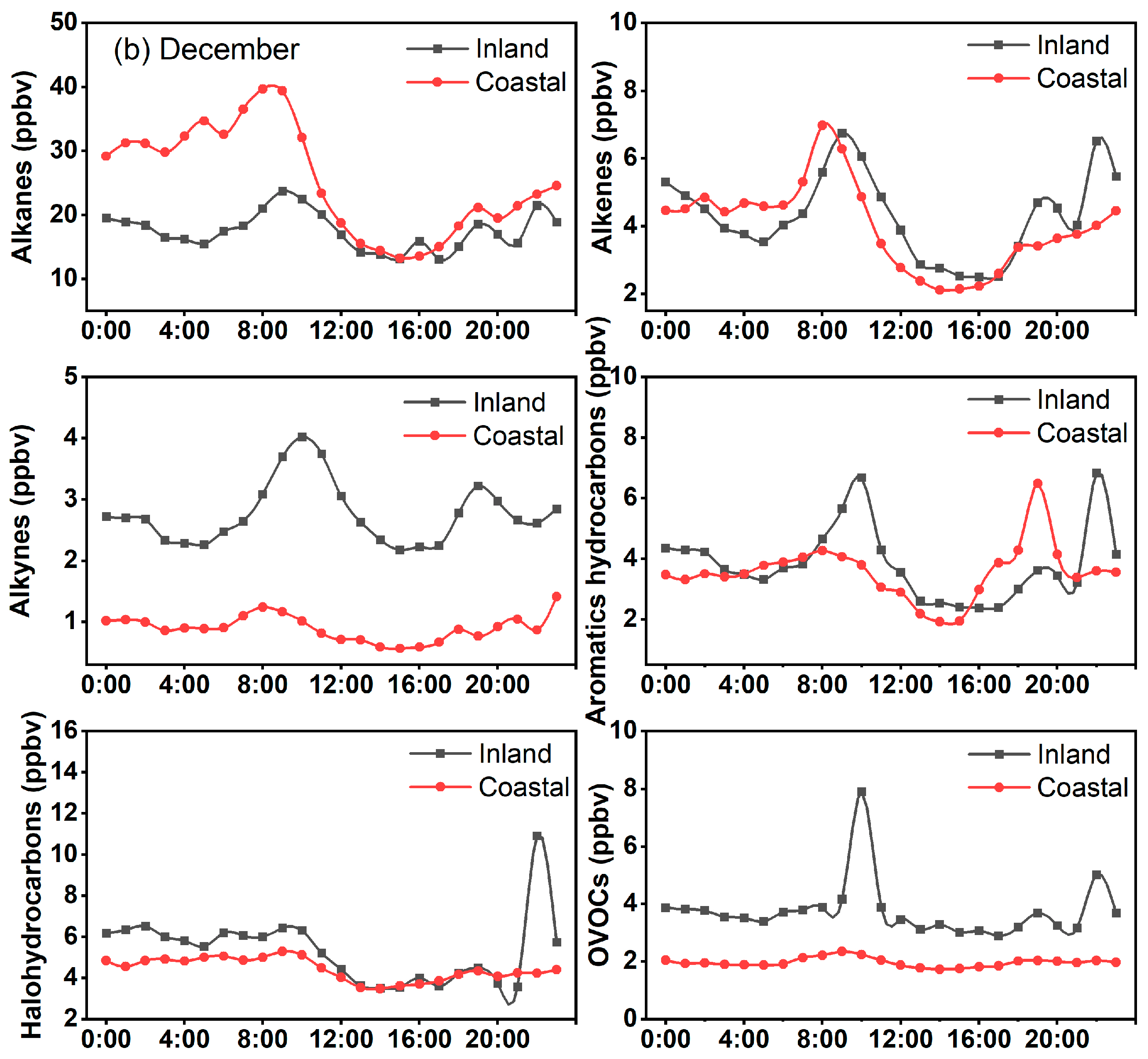
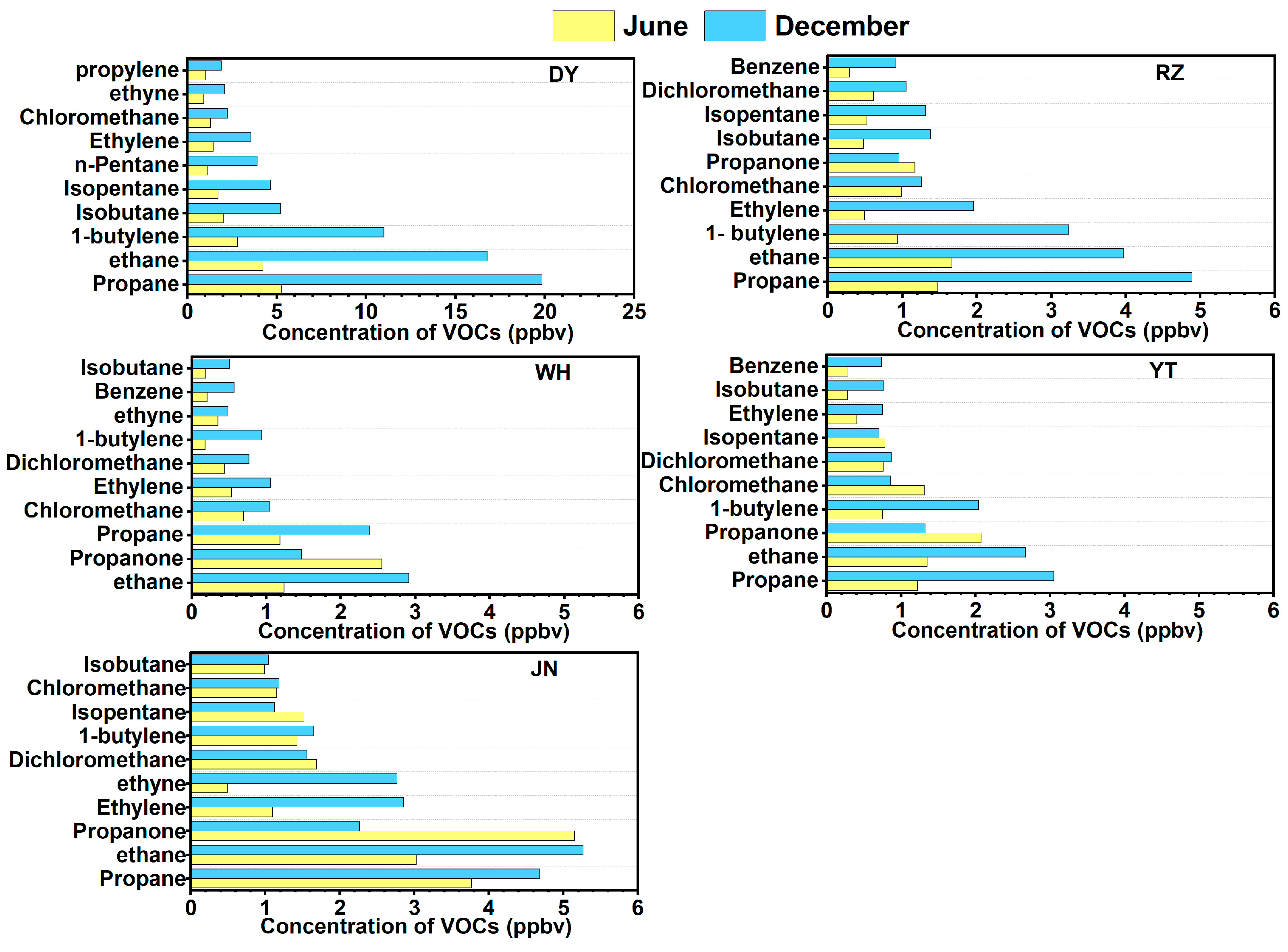
3.1. Temporal Pattern of VOCs

As shown in Figure 2, the concentrations of VOCs in the inland city JN in summer and winter were 27.10 ± 16.44 and 39.90 ± 38.52 ppbv, respectively, which were higher than the coastal cities (RZ, YT, and WH), while VOC concentrations in the coastal city DY (36.01 ± 23.76 and 96.11 ± 78.84 ppbv) were higher than those of inland cities. Additionally, VOC concentrations in coastal and inland cities in winter were higher than those in summer. Comparing different groups of VOCs, alkanes contribute the most in each city. The maximum concentration of alkanes was 67.99 ± 66.09 ppbv in DN in winter. C₂–C₄ alkanes mainly originate from the use and volatilization of NG/LPG [24], indicating that volatile chemicals from oil fields in DN exerted considerable influence on VOCs. Compared with summer (14–28%), the percentage of OVOCs was significantly lower in winter (3–11%), which is consistent with the findings of other regions [25]. It was found that photochemical reactions make an important contribution to the production of carbonyls [26], indicating that the photochemical reaction rate is lower in winter than in summer due to reduced solar radiation and lower temperature. It is worth noting that both average temperature (28.53 °C) and solar radiation (12.23 W/m²) in summer is much higher than wintertime (7.30 °C of average temperature and solar radiation as low as 3.95 W/m²) in JN throughout the sampling period, which, therefore, results in lower OVOC concentrations in winter than in summer.

Figure 3 shows the diurnal variations of VOC concentrations in coastal and inland cities during June and December 2021. The concentrations of alkanes, alkenes, alkynes, aromatic hydrocarbons, and halohydrocarbons exhibited a decreasing trend during the daytime and an accumulating trend during the nighttime. In contrast, OVOC concentrations showed an opposite diurnal variation. During the daytime, the atmospheric oxidation capacity increases with increasing temperature and solar radiation, which facilitates photochemical reactions that produce OVOCs while enhancing the consumption of other groups of VOCs [11]. At night, the decrease in planetary boundary layer height caused the accumulation of VOC concentrations. Further, it is noteworthy that the diurnal variation for most groups of VOC concentration exhibits double-peak patterns (e.g., at 6:00–8:00 and 19:00–21:00). Compared to inland cities, the peaks of VOCs in the coastal city occurred about a hour earlier. In winter, the daily variation of the same group of VOCs is similar, but its peaks occur about two hours later than those in summer. This pattern has also been observed in other areas [27]. This phenomenon is influenced by local traffic emissions and planetary boundary layer height changes. The planetary boundary layer state is influenced by the temperature and humidity conditions [28]. Stable boundary layers can develop at nighttime, particularly in winter, which causes pollutants to accumulate [29]. This is possibly due to the fact that the convective boundary layer tends to appear earlier in coastal areas than inland and later in winter than in summer. The concentrations of alkenes and alkynes in coastal areas during summer showed similar diurnal variations, showing several concentration peaks during the daytime (e.g., at 8:00, 10:00, 13:00, and 16:00). This pattern indicates that alkenes and alkynes might originate from the same sources.

The concentrations of the top 10 VOC species in coastal and inland cities are shown in Figure 4. Alkanes were the most abundant group in the top 10 VOCs in coastal and inland cities. In contrast to other cities, n-pentane (1.15–3.91 ppbv) and propylene (1.04–1.91 ppbv) are found exclusively in DY. It has been reported that n-pentane and propylene are the major VOC emission components in oil refineries [30]. This revealed that the VOC concentration in DY is predominantly influenced by the local oil field extraction. The components with high concentrations of VOCs in RZ are propane (1.47–4.89 ppbv), ethane (1.66–3.97 ppbv), and n-butane (0.93–3.23 ppbv). Propane, ethane, and acetone were the top three concentrations of VOCs in WH, YT, and JN.

The concentrations of many species are substantially higher in winter than in summer. Conversely, the concentration of acetone is higher in summer than in winter, which is likely due to the effects of emission enhancement from vegetation and the production by oxidation of biogenic hydrocarbons in summer [31]. However, isopentane concentrations in JN and YT were slightly higher in summer than in winter. Isopentane was the main component of the evaporative emissions of motor vehicles [32], with higher temperatures in summer increasing the evaporative emissions of isopentane from motor vehicles. This demonstrates that VOCs in JN and YT are affected by motor vehicle emissions. Additionally, the concentration of dichloromethane in JN and chloromethane in YT is slightly higher in summer than in winter. Dichloromethane and chloromethane were substantial in the chemical industry [33], especially in chlorinated chemical plants [34]. Their concentrations vary in relation to the intensity of urban chemical industry emissions. In conclusion, the major species differences of VOCs between coastal and inland cities are not significant, which is mainly influenced by indigenous emission sources.

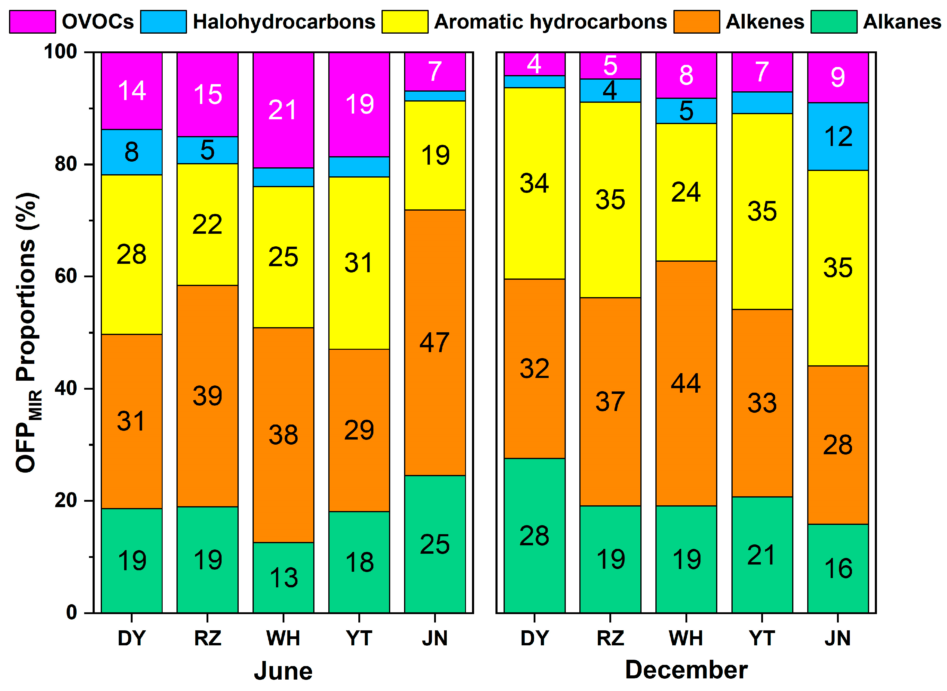
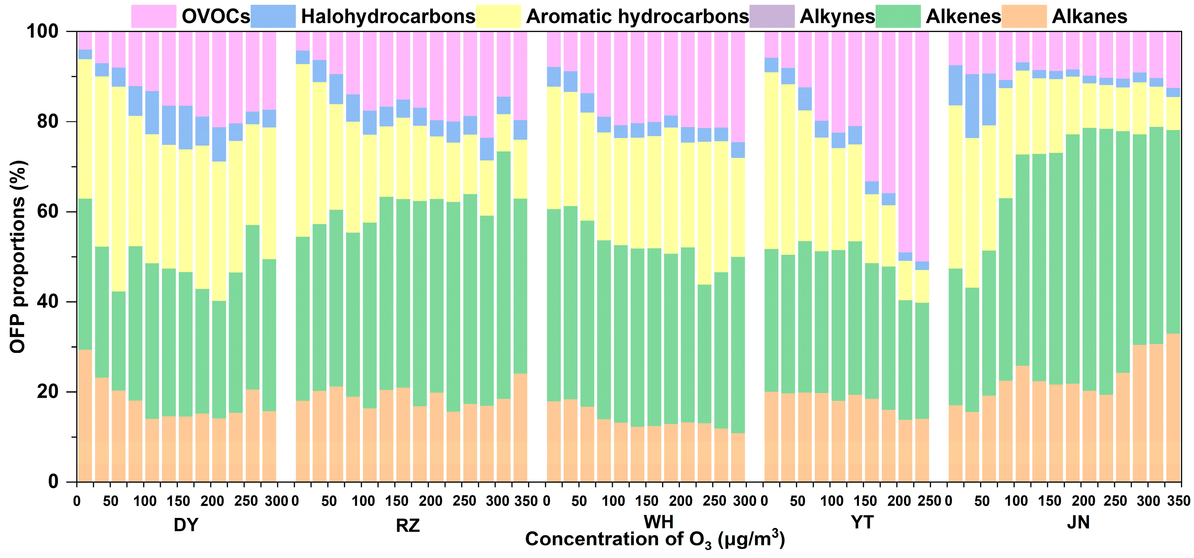
3.2. Chemical Reactivity of VOCs

As important precursors of O₃, it is necessary to study the chemical reactivity of VOCs and analyze their effects on O₃ production. The contributions of different groups of VOCs to OFP_MIR among different cities during summer and winter are shown in Figure 5.

Table 1. Top ten species of VOCs in June and December with their OFP_MIR proportions (%) in Jinan (JN), Dongying (DY), Rizhao (RZ), Yantai (YT), and Weihai (WH).

DY	June	December	Variation (%)	RZ	June	December	Variation (%)
m-Xylene + p-Xylene	5.19	15.01	189.02	m-Xylene + p-Xylene	7.91	17.23	117.88
propylene	9.01	7.73	−14.21	Ethylene	6.85	11.57	68.89
Ethylene	6.50	7.37	13.47	1-butylene	11.05	9.60	−13.12
Butadiene	3.27	8.68	165.25	propylene	4.22	7.95	88.43
1-butylene	3.30	6.04	82.85	1-butylene	3.41	5.06	48.25
methylbenzene	3.70	4.67	26.10	trans-2-butene	7.23	3.32	−54.09
ortho-Xylene	2.72	4.60	68.87	methylbenzene	2.44	5.03	105.92
Isopentane	3.19	4.00	25.33	ortho-xylene	2.22	4.46	100.95
1-butylene	2.05	4.49	119.14	Propionaldehyde	7.04	2.13	−69.70
Propane	2.01	3.53	75.82	cis-2-butene	6.32	2.30	−63.64
WH	June	December	Variation (%)	YT	June	December	Variation (%)
Ethylene	6.48	15.96	146.45	m-Xylene + p-Xylene	12.93	11.63	−10.00
propylene	5.41	13.17	143.24	propylene	5.48	9.72	77.35
1,2,4-trimethylbenzene	11.58	0.79	−93.16	Ethylene	6.23	7.57	21.42
m-Xylene + p-Xylene	5.27	7.27	38.12	1-butylene	1.81	8.69	379.49
1-butylene	4.01	7.39	84.23	methylbenzene	2.69	8.04	198.61
cis-2-butene	6.57	2.45	−62.72	Propionaldehyde	9.74	1.96	−79.86
Propionaldehyde	5.81	2.77	−52.33	1-butylene	3.06	5.43	77.69
trans-2-butene	7.33	0.86	−88.29	ortho-xylene	3.94	4.54	15.44
methylbenzene	1.54	5.23	239.69	Isopentane	4.98	2.93	−41.20
butyraldehyde	4.35	0.69	−84.23	Isoprene	5.21	0.56	−89.32
JN	June	December	Variation (%)
Ethylene	10.06	12.32	22.40
m-Xylene + p-Xylene	6.11	10.12	65.57
methylbenzene	5.23	5.97	14.20
1-butylene	14.03	1.78	−87.30
propylene	6.05	5.16	−14.81
ortho-xylene	2.50	4.17	66.83
Isopentane	5.76	2.00	−65.19
Isoprene	6.71	1.50	−77.64
1-butylene	3.46	1.88	−45.64
1,2,4-trimethylbenzene	1.01	2.81	176.46

presents the seasonal variation of the top ten VOC species contributing to OFP_MIR.

As shown in Figure 5, the contribution of aromatic hydrocarbons and alkenes to OFP_MIR was significant among different cities. This result was also found in other inland [35] and coastal [36] regions. In DY and JN, alkenes were shown to have made the largest contribution (31% and 47%) to O₃ formation in summer, and the contribution of aromatic hydrocarbons in winter increased with 34% and 35%, respectively. RZ and WH have the highest contribution of alkenes in both summer and winter, with 39% and 38% in summer and 37% and 44% in winter. Aromatic hydrocarbons accounted for 31% and 35% of OFP_MIR in YT during winter and summer, respectively. In addition, the contribution of OVOCs to O₃ production was more significant in coastal cities in summer compared to inland cities. The results of the top 10 VOC species contributing to OFP_MIR (Table 1) showed that m-Xylene + p-Xylene makes the highest contribution to OFP_MIR in coastal cities DY (5.19–15.01%), RZ (7.91–17.23%) and YT (11.63–12.93%). This is attributed to the high reactivity of aromatic hydrocarbon. Prior studies have shown that m-Xylene + p-Xylene was a predominant component in printing industry solvent [37] and aromatic hydrocarbon was the most abundant species in wood furniture coating [38] and the petrochemical industry [39]. Further analysis regarding the dominant anthropogenic for monitoring sites suggests that the petrochemical industry may exert a profound influence on DY, and emissions from gas stations may have significant impacts on RZ, WH, and YT. For JN, construction paint may emerge as the dominant contributor due to intense construction activities. In addition, ethylene (6.23–15.96 ppbv) and methylbenzene (1.58–8.04 ppbv) contribute significantly to O₃ production in both inland and coastal cities. Ethylene (11.80%) and methylbenzene (11.27%) were the most abundant VOCs in exhaust gas from on-road vehicles [40]. This suggests that the contribution of vehicle emissions to O₃ production in NCP should not be neglected. The components with high proportional contributions to O₃ formation in WH were ethylene (6.48–15.96%), propylene (5.41–13.17%) and 1,2,4-trimethylbenzene (0.79–11.58%). In coastal regions, ship exhaust emissions contributed significantly to anthropogenic sources of VOCs, with ethylene and 1,2,4-trimethylbenzene being the main species emitted [41]. This indicates that ship emissions have a relatively large influence on O₃ formation in WH. As the dominant species of biogenic source [42], isoprene contributes to O₃ production in JN and YT during summer, with contributions reaching 6.71% and 5.21%, respectively.

To investigate the influence of VOCs on O₃ formation intensity, the contribution of VOCs OFP_MIR at different O₃ concentration levels was calculated. Figure 6 shows the variation in OFP_MIR proportions of the VOC groups with the concentration of O₃. In coastal areas, especially YT, the percentage of OVOC OFP_MIR increased greatly as O₃ concentration increased, while this phenomenon was not significant in inland areas. This phenomenon is likely influenced by the atmospheric oxidation capacity, which was found to be positively correlated with O₃ concentration in a previous study [43]. The increasing atmospheric oxidation capacity promotes the secondary production of OVOCs [44]. As with the increase in O₃ concentration, the OFP_MIR proportion of aromatic hydrocarbons decreased in RZ, YT, and JN. In DY and WH, alkenes and aromatic hydrocarbons consistently accounted for high proportions of OFP_MIR. In JN and RZ, alkenes contribute the most to O₃ formation, and contributions of both alkenes and alkanes increase with the increase in O₃ concentrations, indicating that O₃ formation in these two cities is mainly influenced by alkenes.

3.3. Model Simulation of O₃ Photochemical Formation

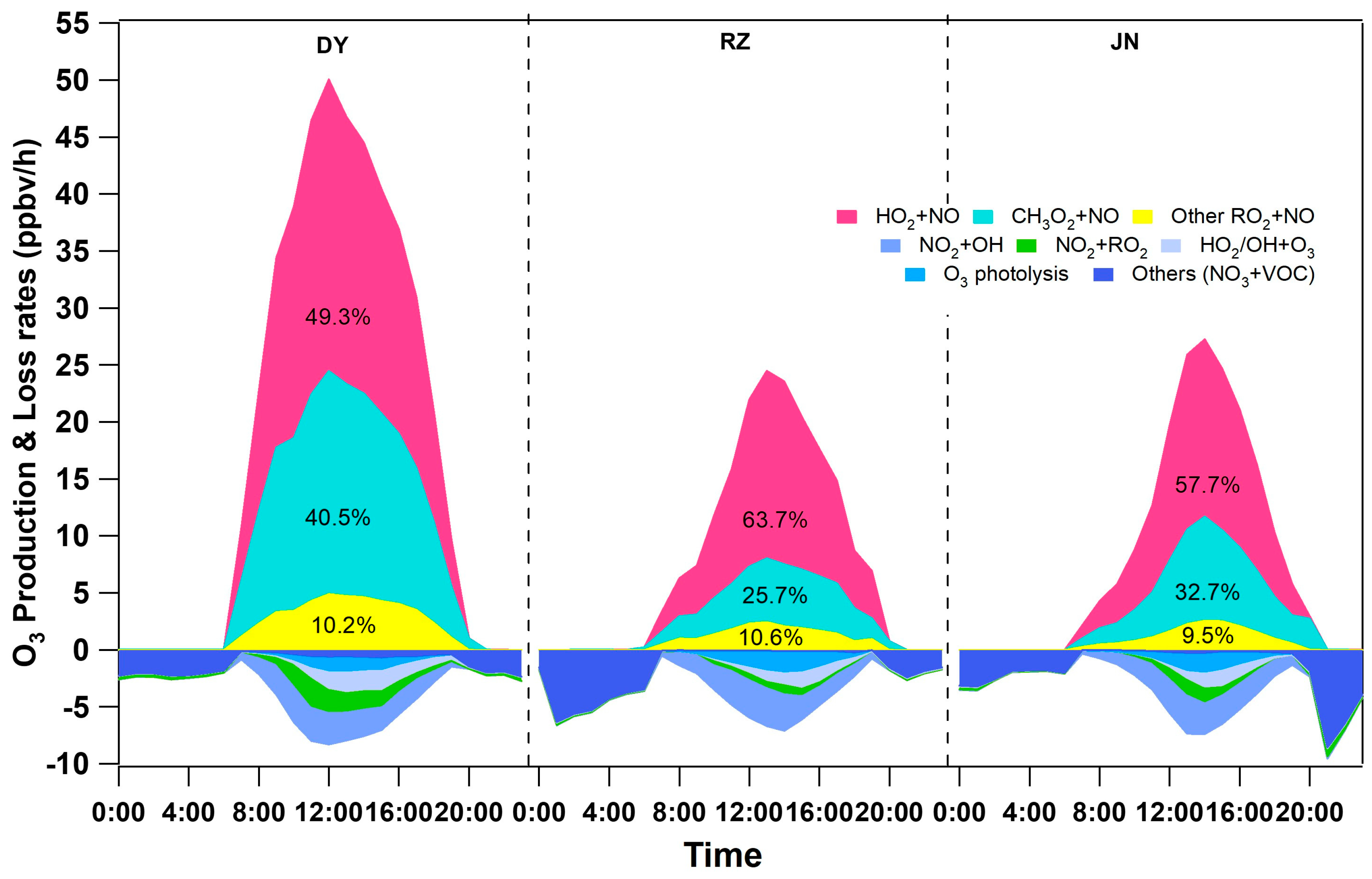
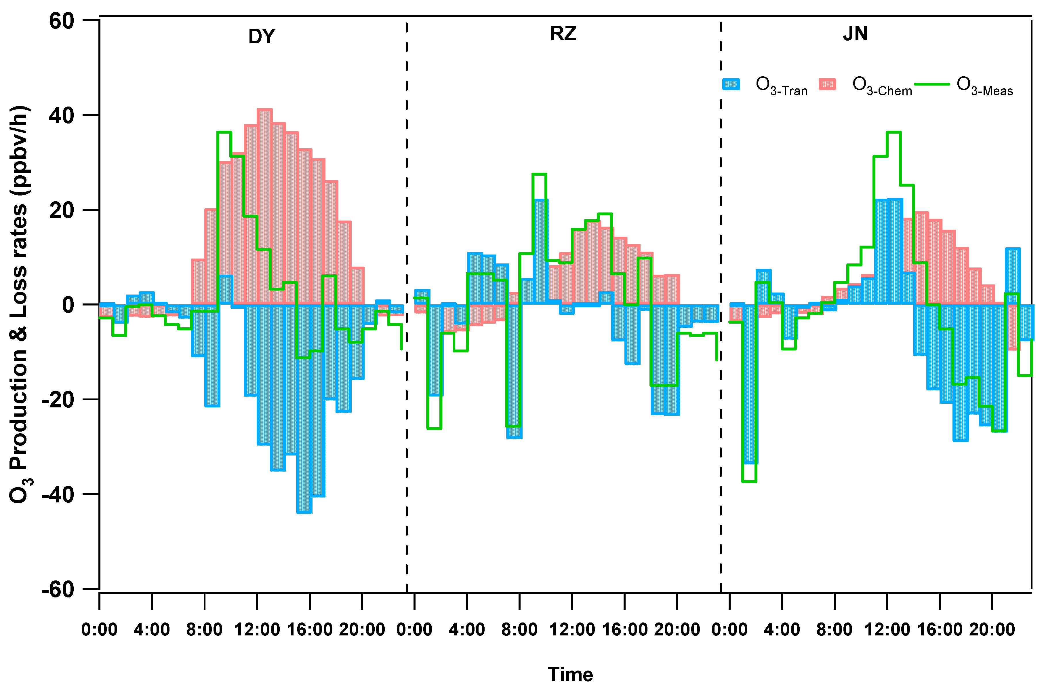
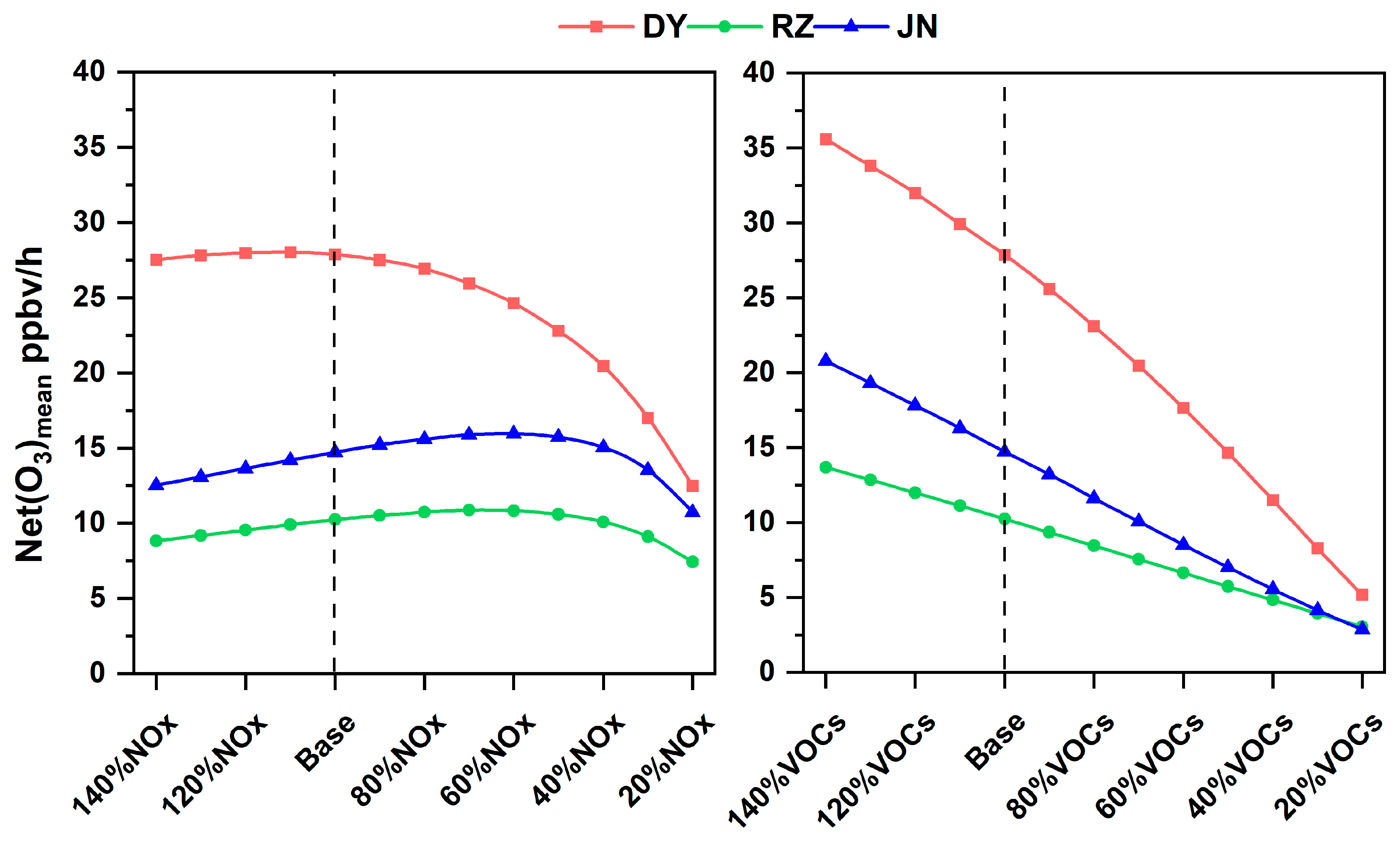
3.3.1. O₃ Formation Based on MCM Modeling

In order to understand the causes of O₃ pollution in different cities from the perspective of chemical reaction pathways, the typical coastal cities DY and RZ and the inland city JN were selected for comparison. O₃ production was simulated based on MCM for these cities on days with high O₃ concentration (DY: 6 June; RZ: 22 June; JN: 8 June). Figure 7 showed the in situ O₃ photochemistry production mechanism on high O₃ pollution days. It was found that the net O₃ production rates in DY, RZ, and JN were 27.87, 10.24, and 10.37 ppbv/h, respectively. This is comparable to the research from another coastal city Xiamen, where the net O₃ production rate was 9.1 ppbv/h [45]. The pathway that contributed most to O₃ production was HO₂ + NO, which had daytime contribution rates of 16.43, 8.98, and 8.19 ppbv/h in DY, RZ, and JN, accounting for 49.29%, 63.66%, and 57.72%, respectively. RO₂ + NO is another pathway with a significant contribution to O₃ production, which is divided into CH₃O₂ + NO with the largest contribution and other RO₂ + NO. The rate of CH₃O₂ + NO was 13.50, 3.63, and 4.67 ppbv/h, accounting for 40.50%, 25.72%, and 32.74%, respectively.

According to the results of the O₃ production pathway, the O₃ production rate in DY (27.87 ppbv/h) is significantly higher than that in the coastal city RZ (10.24 ppbv/h) and the inland city JN (10.37 ppbv/h). The O₃ production pathways in RZ and JN are dominated by HO₂ + NO, while the RO₂ + NO contributes the most to O₃ production in DY. This is mainly caused by the large contribution of the CH₃O₂ + NO (40.50%). CH₃O₂ is the dominant species of RO₂, and it was found that CH₃O₂ accounts for 83% of RO₂. CH₃O₂ is mainly derived from CH₄(OH + CH₄ → CH₃O₂), and CH₃O₂ can react with NO to produce HO₂(CH₃O₂ + NO → HCHO + HO₂ + NO₂), which propagates the HO_X radical and further O₃ production [46,47]. Moreover, it has also been shown that oil extraction is the principal source sector of CH₄. Therefore, it is speculated that the emissions from the oilfield promote the enrichment of CH₄, which further promotes the reaction of CH₃O₂ with NO, resulting in a higher rate of in situ O₃ production in DY.

The abovementioned analysis shows that the in situ O₃ production rate is different from the observed O₃ concentration variation. This is because the O₃ concentration variation is affected by a combination of in situ photochemical reactions and physical processes [22,23]. The diurnal variation of the net O₃ production rate (O_3-Chem) and regional transport O₃ (O_3-Tran) as well as the observed O₃ production change rate (d(O₃/dt)) in cities during the O₃ pollution process are shown in Figure 8. The rate of O₃ change was calculated from the derivative of the observed O₃ time series (O_3-meas = d(O₃)/dt). The rate of in situ O₃ production (O_3-chem) is calculated based on the MCM model. The difference between them is the rate of O₃ change for physical transport (O_3-tran = O_3-meas − O_3-chem), which incorporates horizontal regional transport and the role of the atmospheric mixed layer [22,23]. To understand the effect of regional transport on O₃ concentration, the spatial distribution of temperature and wind vectors during the O₃ pollution process in Shandong Province was simulated based on the WRF-Chem model shown in Figure 9.

O_3-tran > 0 indicates inward transport and O_3-tran > 0 indicates outward transport. The transport contributes more to the O₃ concentration in the morning in RZ (8:00–9:00) and JN (8:00–12:00), which is due to the contribution of residual boundary-layer air [48] to O₃. In DY, O₃ concentrations are mainly influenced by in situ production and there is a clear trend of outward export in the afternoon, combined with Figure 9, which shows that it is mainly influenced by easterly winds originating from the ocean and with high wind speed. RZ was influenced by winds from the northeast with low wind speed, where regional transmission has less influence on O₃ concentrations. JN has a larger O₃ transmission in the afternoon and is influenced by southeast transmission from the inland regions.

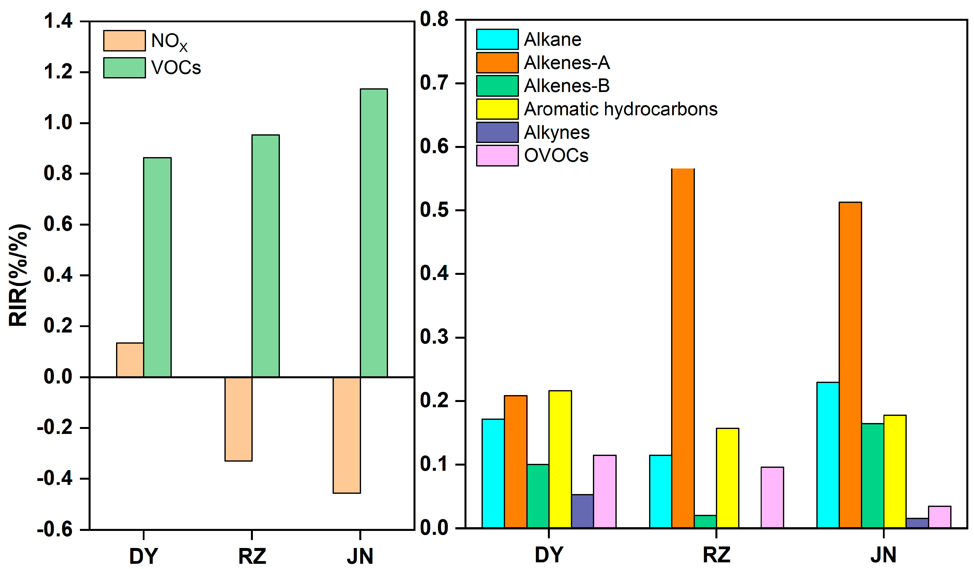
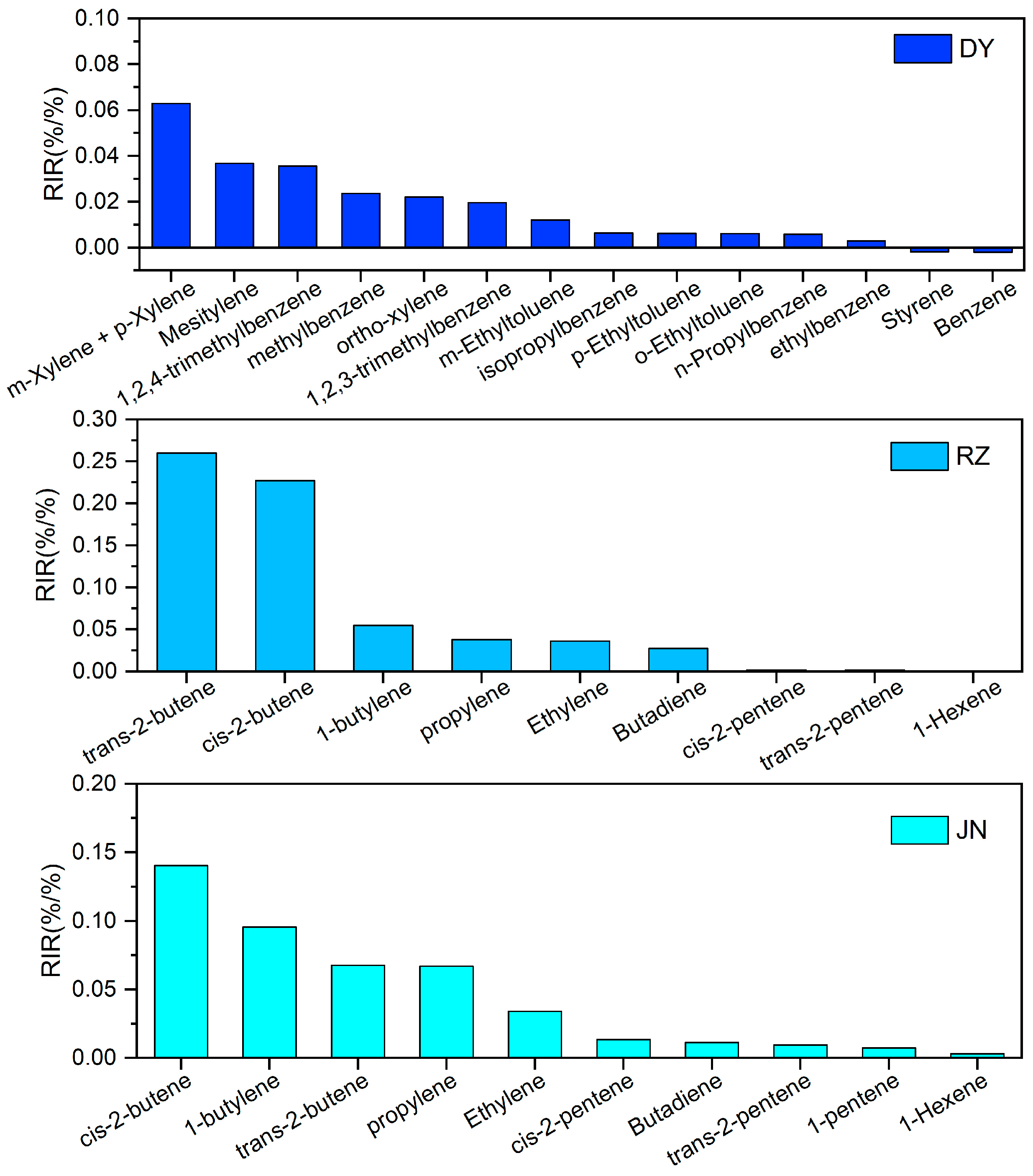
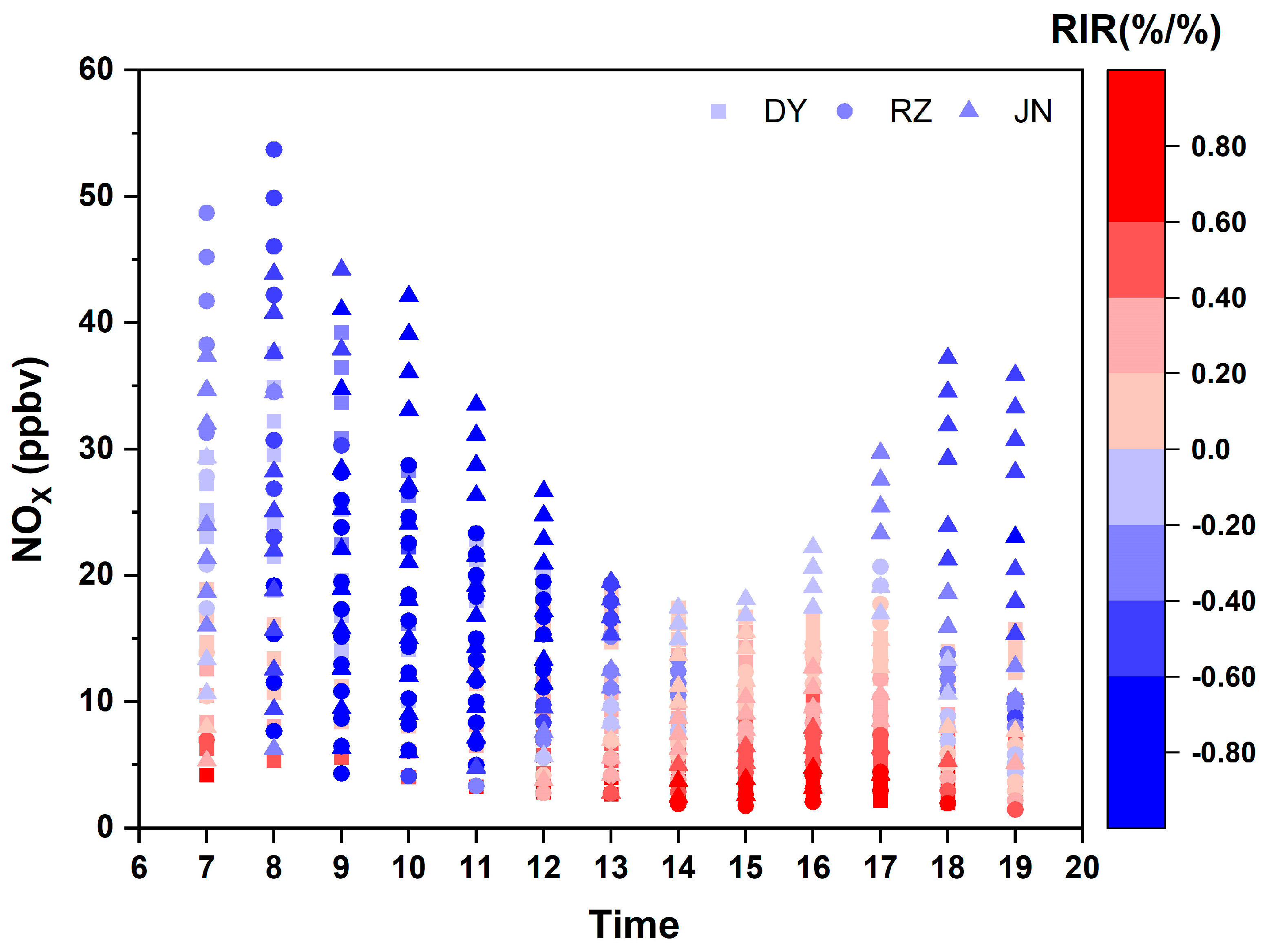
3.3.2. RIR of NOx and VOCs

The simulation of sensitive species abatement scenarios are conducted using model-controlled O₃ production, i.e., the rate of change in O₃ production rates caused by a hypothetical 20% reduction in the concentration of specific O₃ precursors (VOCs and NOx), respectively. The RIR and abatement response are explained by applying the O₃ production mechanism during the observation period [49].

As shown in Figure 10, the formation of high O₃ pollution in DY is limited by VOCs and NOx, while the O₃ production in JN and RZ is mainly the VOC-limited regime. The results of sensitivity experiments undertaken by reducing the concentration of VOCs by 20% showed that the O₃ reduction rates were 15.95%, 20.83%, and 17.19%, respectively. Further sensitivity experiments were conducted by reducing the concentration of different groups of VOCs by 20%. Additionally, Isoprene was classified as a biogenic alkene (alkene-B) and the other alkenes were categorized as anthropogenic alkenes (alkene-A). Controlling the concentration of aromatic hydrocarbons and alkenes-A could significantly reduce the O₃ formation in DY, and the O₃ reduction rates were calculated to be 3.96% and 3.82%. In JN and RZ, controlling alkenes-A could significantly reduce the O₃ formation with O₃ reduction rates of 9.12% and 12.74%, respectively. In addition, controlling alkane concentrations can also reduce O₃ production, with RIRs of 0.17, 0.11, and 0.23 in DY, RZ, and JN, respectively. Compared to coastal cities, inland city JN O₃ production was more sensitive to alkene-B, with an RIR of 0.16. In contrast, O₃ production was more sensitive to OVOCs, with RIRs of 0.11 and 0.10 in coastal regions DY and RZ, respectively. Therefore, alkenes and aromatic hydrocarbons are the key groups that have a large impact on O₃ production during periods of heavy O₃ pollution. In DY, reducing aromatic hydrocarbons and alkenes can effectively mitigate O₃ pollution, and in JN and RZ, reducing alkene concentrations can reduce O₃ pollution. This conclusion is consistent with the results of the OFP analysis in 3.2 (Figure 5 and Figure 6).

To investigate the effect of individual species on O₃ production, sensitivity experiments were conducted on individual species of the most sensitive VOC species in each city. As shown in Figure 11, in DY, the most sensitive species among aromatic hydrocarbons was m-Xylene + p-Xylene, followed by mesitylene, 1,2,4-trimethylbenzene, and methylbenzene. The species with the highest contribution to O₃ production among alkenes was butene, in JN and RZ. Moreover, trans-2-butene, cis-2-butene, and 1-butylene made a significant contribution to O₃ production in RZ with RIRs of 0.26, 0.23, and 0.05, respectively. It was found that decreasing the concentration of cis-2-butene, 1-butylene, and trans-2-butene led to the greatest change in O₃ production rate at JN, with RIRs of 0.14, 0.95, and 0.07, respectively. This result is consistent with previous studies in Zibo [19], where C₂–C₅ alkenes and C₇–C₉ aromatic hydrocarbons contributed greatly to O₃ production. It was found that aromatic hydrocarbons were the characteristic compounds of architectural coatings and solvents [50], and cis-2-butene, 1-butylene, and trans-2-butene all originate from vehicle exhaust and liquefied petroleum gas (LPG) [51]; therefore, cities should further implement targeted control of their emissions.

The results of sensitivity experiments showed that the effect of important precursors of O₃ (NO_X and VOCs) on O₃ production varies in different contexts. O₃ production rate increases with the decrease of NO_X concentrations, and the relationship between O₃ and NO_X is complex. Therefore, this study further simulates the O₃ production rate in the set of assumed NO_X and VOCs with different concentration gradients, i.e., NO_X and VOC concentrations are respectively reduced by 10–80% and increased by 10–40%, then input to the model for simulation. The net O₃ production rates for different abatement scenarios are shown in Figure 12, and the corresponding RIRs are given in

Table 2. Relative incremental reactivity (RIR) of different reduction ratios of NO_X and VOCs in Dongying (DY), Rizhao (RZ), and Jinan (JN) (%/%).

Reduction Ratios		140%	130%	120%	110%	90%	80%	70%	60%	50%	40%	30%	20%
NOx	DY	−0.027	−0.004	0.019	0.040	0.151	0.173	0.237	0.300	0.373	0.454	0.566	0.699
	RZ	−0.350	−0.355	−0.364	−0.340	−0.304	−0.301	−0.283	−0.234	−0.181	−0.108	0.014	0.193
	JN	−0.402	−0.413	−0.407	−0.404	−0.424	−0.391	−0.378	−0.339	−0.282	−0.198	−0.052	0.183
VOCs	DY	0.704	0.721	0.749	0.733	0.837	0.867	0.896	0.924	0.955	0.983	1.007	1.019
	RZ	0.920	0.927	0.925	0.928	0.951	0.945	0.943	0.938	0.939	0.934	0.928	0.921
	JN	1.118	1.131	1.133	1.152	1.098	1.121	1.113	1.101	1.089	1.071	1.050	1.025

.

Different concentration gradients of emission reduction revealed that O₃ production in three cities was more sensitive to VOCs compared to NO_X, and reducing VOC concentration can lead to a significant reduction in net O₃ production rate. Based on the slope (Figure 12), it can be concluded that O₃ production in DY is the most sensitive to VOC emission reduction. Further, based on the RIR values in response to the varied reduction ratio (Table 2), it is seen that RIR values increase with the incremental reduction of VOCs in DY, which indicates a higher reduction rate of O₃ production. However, the scenario of 10% abatement of VOC concentration in RZ has the most significant effect on O₃ production, with an RIR of 0.951. In contrast, the response of emission reduction in JN is much more complex. In the context of reducing VOC concentration, when VOC concentration is reduced by 20%, O₃ sensitivity is the highest, and the RIR is 1.12. However, a 10% increase in VOC concentration has a stronger O₃ production response, with an RIR of 1.15. This situation indicates that VOC emission in JN can lead to a significant increase in the O₃ production rate.

The response of the net O₃ production rate to the change of NO_X concentration in each city is not evident, and sensitivity is ranked as follows: DY > JN > RZ. Reducing NO_X concentration in DY can lead to a lower O₃ production rate, and the RIR peaks at 0.699 when the NO_X concentration is multiplied by 20%. The O₃ production rate also decreases when NO_X concentration increases by more than 30%. In RZ and JN, O₃ production rate would decrease only when the NO_X reduction ratio is more than 60% and 70%, respectively. When the NO_X concentration is reduced by 80%, the RIR reaches the maximum value of 1.93 and 1.83, respectively. The phenomenon by means of which increasing NO_X concentration decreases the O₃ production rate indicates that NO_X concentration plays a titration role in O₃ production [52]. The difference in O₃ production rates between cities with respect to NO_X sensitivity in this study, which is postulated to be related to the differences in NO_X concentrations in different cities, deserves further investigation.

To better understand the relationship between NO_X concentration and O₃ production rate, the hourly simulation results of different cities are summarized. Figure 13 shows the distribution of NO_X concentration change and RIR during the daytime (7:00–19:00). The effect of NO_X concentration on the change of O₃ production rate is expressed by RIR; when RIR is positive, it means that the change of NO_X concentration is positively correlated with the O₃ production rate, and vice versa, it is negatively correlated, and the magnitude of the absolute value of RIR indicates the magnitude of sensitivity. An important phenomenon was also demonstrated, which was a negative RIR in the morning (9:00–11:00) and a positive RIR in the afternoon (15:00–17:00) with greater sensitivity at lower NO_X concentrations. This phenomenon was also found in other studies, where O₃ production in California shifted towards a more NO_X-sensitive scenario in the afternoon [53], indicating that when the NO_X concentration is at a high level in the morning, the effect on the O₃ production rate is negatively correlated, i.e., reducing the NO_X concentration will decrease the titration effect on O₃ production, resulting in elevated ozone concentration. Conversely, greater efficiency of O₃ reduction could be achieved by reducing NO_X when the NO_X concentration is low (less than 20 ppbv in this study) in the afternoon.

4. Discussion

In this study, we measured VOCs by GC-MS in five cities over the NCP for two sampling periods (June and December) in 2021. The detailed chemical composition and reactivity of VOCs are investigated and the implications for O₃ formation are examined using the OBM.

Previous studies have investigated VOC components which have a single sampling point location and brief sampling period. In this study, different coastal and inland cities were purposely selected and a large amount of data was comprehensively analyzed. Consistent with the findings of other regions [10,25], alkanes contribute the most to VOCs in NCP; however, the alkanes accounted for 71% of VOCs in DY during winter, which was significantly higher than previous studies (45.88%) [54]. This was caused by the volatile emissions from oil fields in DY. The major species differences of VOCs between coastal and inland cities, which are mainly influenced by indigenous emission sources, are not significant.

It is found that the differences in VOC composition between cities not only affect the O₃ potential but also the main pathways of O₃ production. The O₃ production rate in DY (27.87 ppbv/h) is significantly higher than that in the coastal city RZ (10.24 ppbv/h) and Xiamen (9.1 ppbv/h) [45]. The O₃ production pathways in RZ and JN are dominated by HO₂ + NO, while RO₂ + NO contributes the most to O₃ production in DY. It is speculated that oil field emissions promote the enrichment of CH₄, which further promotes the reaction of CH₃O₂ with NO [46,47], resulting in a higher rate of in situ O₃ production in DY. Furthermore, our results suggest that the O₃ abatement response sensitivities are impacted by differences in VOCs and NOx concentrations. The response between O₃ and NO_X has a clear daily variation pattern (the sensitivity is greater from 15:00 to 17:00 in the afternoon), which was also found in California [53].

The major limitation of the present study is that, apart from isoprene, we did not measure biogenic VOCs, which contribute greatly to O₃ formation. Moreover, the identification of dominant anthropogenic emission sources in monitoring sites is limited to emission features, and thereby requires quantitative source apportionment from chemical transport models. Therefore, an expanded ambient monitoring network with routine measurements of VOCs (biogenic and anthropogenic) and high-resolution chemical transport modeling are needed to further elucidate the characteristics of VOCs and their effect on O₃ formation.

5. Conclusions

In this study, we characterize the spatial and temporal patterns of VOCs and investigate the O₃ production mechanism on an O₃ pollution day over the NCP region. For the temporal distribution of VOCs, except OVOCs, the concentrations of VOCs are greatly higher in winter than summer and the daily variation shows a pattern of decreasing during the daytime and accumulating during the nighttime, while the seasonal and diurnal variation patterns of OVOC concentrations are the opposite. The peaks of VOC diurnal concentration in the coastal city occurred earlier compared with inland city. Alkanes accounted for the largest proportion of VOCs in cities, particularly in DY, where alkanes contributed 71% of VOCs, which were affected by oil field emissions. The chemical reactivity of VOCs suggests that aromatic hydrocarbons and alkenes contribute most to OFP in NCP. In addition, compared to inland cities, the contribution of OVOCs to O₃ production was more significant in coastal cities during summer.

The in situ O₃ photochemistry production mechanism on high O₃ pollution days showed that net O₃ production rates in DY, RZ, and JN were 27.87, 10.24, and 10.37 ppbv/h. The pathway that contributed most to O₃ production was HO₂ + NO, followed by RO₂ + NO (CH₃O₂ + NO and other RO₂ + NO). The formation of high O₃ pollution in DY in summer was the transitional regime, but it’s VOC-limited in JN and RZ. Alkenes and aromatic hydrocarbons are the key groups that have a large impact on O₃ production during periods of heavy O₃ pollution. Reducing aromatic hydrocarbons (m/p-xylene) and alkenes (butene) can effectively mitigate O₃ pollution in NCP.

Different concentration gradients of emission reduction revealed that O₃ production in DY is the most sensitive to VOCs emission reduction. The response of the net O₃ production rate to the change in NO_X concentration is not obvious, and the sensitivity is DY > JN > RZ. The response between O₃ and NO_X is influenced by the NO_X concentration and has a clear daily variation pattern (the sensitivity is greater from 15:00 to 17:00 in the afternoon). The greatest efficiencies in O₃ reduction could be achieved by reducing NO_X when the NO_X concentration is low (less than 20 ppbv in this study).

References

1. Tao, T.; Shi, Y.; Gilbert, K.M.; Liu, X. Spatiotemporal variations of air pollutants based on ground observation and emission sources over 19 Chinese urban agglomerations during 2015–2019. Sci. Rep. 2022, 12, 2045–2322. [Google Scholar] [CrossRef]
2. Li, X.; Chen, Q.; Zheng, X.; Li, Y.; Han, M.; Liu, T.; Xiao, J.; Guo, L.; Zeng, W.; Zhang, J.; et al. Effects of ambient ozone concentrations with different averaging times on asthma exacerbations: A meta-analysis. Sci. Total Environ. 2019, 691, 549–561. [Google Scholar] [CrossRef] [PubMed]
3. Zhang, Y.; Tian, Q.; Wei, X.; Feng, X.; Ma, P.; Hu, W.; Xin, J.; Ni, C.; Wang, S.; Zheng, C. Temperature modulation of adverse consequences of ozone exposure on cardiovascular mortality: A study of multiple cities in China. Atmos. Environ. 2022, 288, 119272. [Google Scholar] [CrossRef]
4. Jurán, S.; Edwards-Jonášová, M.; Cudlín, P.; Zapletal, M.; Šigut, L.; Grace, J.; Urban, O. Prediction of ozone effects on net ecosystem production of Norway spruce forest. iForest-Biogeosci. For. 2018, 11, 743–750. [Google Scholar] [CrossRef]
5. Juráň, S.; Grace, J.; Urban, O. Temporal Changes in Ozone Concentrations and Their Impact on Vegetation. Atmosphere 2021, 12, 82. [Google Scholar] [CrossRef]
6. Wei, W.; Wang, X.; Wang, X.; Li, R.; Zhou, C.; Cheng, S. Attenuated sensitivity of ozone to precursors in Beijing–Tianjin–Hebei region with the continuous NOx reduction within 2014–2018. Sci. Total Environ. 2022, 813, 152589. [Google Scholar] [CrossRef]
7. Sha, Q.; Zhu, M.; Huang, H.; Wang, Y.; Huang, Z.; Zhang, X.; Tang, M.; Lu, M.; Chen, C.; Shi, B.; et al. A newly integrated dataset of volatile organic compounds (VOCs) source profiles and implications for the future development of VOCs profiles in China. Sci. Total Environ. 2021, 793, 148348. [Google Scholar] [CrossRef]
8. Feng, Y.; An, J.; Tang, G.; Zhang, Y.; Wang, J.; Lv, H. Characteristics and Sources of Volatile Organic Compounds in the Nanjing Industrial Area. Atmosphere 2022, 13, 1136. [Google Scholar] [CrossRef]
9. Sun, J.; Shen, Z.; Wang, R.; Li, G.; Zhang, Y.; Zhang, B.; He, K.; Tang, Z.; Xu, H.; Qu, L.; et al. A comprehensive study on ozone pollution in a megacity in North China Plain during summertime: Observations, source attributions and ozone sensitivity. Environ. Int. 2021, 146, 106279. [Google Scholar] [CrossRef]
10. Wang, Z.; Wang, H.; Zhang, L.; Guo, J.; Li, Z.; Wu, K.; Zhu, G.; Hou, D.; Su, H.; Sun, Z.; et al. Characteristics of volatile organic compounds (VOCs) based on multisite observations in Hebei province in the warm season in 2019. Atmos. Environ. 2021, 256, 118435. [Google Scholar] [CrossRef]
11. Ji, X.; Xu, K.; Liao, D.; Chen, G.; Liu, T.; Hong, Y.; Dong, S.; Choi, S.; Chen, J. Spatial-temporal Characteristics and Source Apportionment of Ambient VOCs in Southeast Mountain Area of China. Aerosol Air Qual. Res. 2022, 22, 220016. [Google Scholar] [CrossRef]
12. Liu, Y.; Wang, H.; Jing, S.; Gao, Y.; Peng, Y.; Lou, S.; Cheng, T.; Tao, S.; Li, L.; Li, Y.; et al. Characteristics and sources of volatile organic compounds (VOCs) in Shanghai during summer: Implications of regional transport. Atmos. Environ. 2019, 215, 116902. [Google Scholar] [CrossRef]
13. Wei, J.; Li, Z.; Li, K.; Dickerson, R.R.; Pinker, R.T.; Wang, J.; Liu, X.; Sun, L.; Xue, W.; Cribb, M. Full-coverage mapping and spatiotemporal variations of ground-level ozone (O3) pollution from 2013 to 2020 across China. Remote Sens. Environ. 2022, 270, 112775. [Google Scholar]
14. Zhang, J.; Wang, C.; Qu, K.; Ding, J.; Shang, Y.; Liu, H.; Wei, M. Characteristics of Ozone Pollution, Regional Distribution and Causes during 2014–2018 in Shandong Province, East China. Atmosphere 2019, 10, 501. [Google Scholar] [CrossRef]
15. Sun, J.; Duan, S.; Wang, B.; Sun, L.; Zhu, C.; Fan, G.; Sun, X.; Xia, Z.; Lv, B.; Yang, J.; et al. Long-Term Variations of Meteorological and Precursor Influences on Ground Ozone Concentrations in Jinan, North China Plain, from 2010 to 2020. Atmosphere 2022, 13, 994. [Google Scholar] [CrossRef]
16. Carter, W.P.L. Computer modeling of environmental chamber measurements of maximum incremental reactivities of volatile organic compounds. Atmos. Environ. 1995, 29, 2513–2527. [Google Scholar] [CrossRef]
17. Carter, W.P.L. Updated maximun incremental reactivity scale and hydrocarbon bin reactivities for regulatory applications. Calif. Air Resour. Board Contract 2009, 339, 2009. [Google Scholar]
18. Wang, S.; Tsona, N.T.; Du, L. Effect of NOx on secondary organic aerosol formation from the photochemical transformation of allyl acetate. Atmos. Environ. 2021, 255, 118426. [Google Scholar] [CrossRef]
19. Lin, H.; Wang, M.; Duan, Y.; Fu, Q.; Ji, W.; Cui, H.; Jin, D.; Lin, Y.; Hu, K. O3 Sensitivity and Contributions of Different NMHC Sources in O3 Formation at Urban and Suburban Sites in Shanghai. Atmosphere 2020, 11, 295. [Google Scholar] [CrossRef]
20. Wang, M.; Hu, K.; Chen, W.; Shen, X.; Li, W.; Lu, X. Ambient Non-Methane Hydrocarbons (NMHCs) Measurements in Baoding, China: Sources and Roles in Ozone Formation. Atmosphere 2020, 11, 1205. [Google Scholar] [CrossRef]
21. Zhang, K.; Liu, Z.; Zhang, X.; Li, Q.; Jensen, A.; Tan, W.; Huang, L.; Wang, Y.; de Gouw, J.; Li, L. Insights into the significant increase in ozone during COVID-19 in a typical urban city of China. Atmos. Chem. Phys. 2022, 22, 4853–4866. [Google Scholar] [CrossRef]
22. Li, K.; Wang, X.; Li, L.; Wang, J.; Liu, Y.; Cheng, X.; Xu, B.; Wang, X.; Yan, P.; Li, S.; et al. Large variability of O3-precursor relationship during severe ozone polluted period in an industry-driven cluster city (Zibo) of North China Plain. J. Clean. Prod. 2021, 316, 128252. [Google Scholar] [CrossRef]
23. Xue, L.K.; Wang, T.; Gao, J.; Ding, A.J.; Zhou, X.H.; Blake, D.R.; Wang, X.F.; Saunders, S.M.; Fan, S.J.; Zuo, H.C.; et al. Ground-level ozone in four Chinese cities: Precursors, regional transport and heterogeneous processes. Atmos. Chem. Phys. 2014, 14, 13175–13188. [Google Scholar] [CrossRef]
24. Hui, L.; Liu, X.; Tan, Q.; Feng, M.; An, J.; Qu, Y.; Zhang, Y.; Deng, Y.; Zhai, R.; Wang, Z. VOC characteristics, chemical reactivity and sources in urban Wuhan, central China. Atmos. Environ. 2020, 224, 117340. [Google Scholar] [CrossRef]
25. Wang, F.; Du, W.; Lv, S.; Ding, Z.; Wang, G. Spatial and Temporal Distributions and Sources of Anthropogenic NMVOCs in the Atmosphere of China: A Review. Adv. Atmos. Sci. 2021, 38, 1085–1100. [Google Scholar] [CrossRef] [PubMed]
26. Chen, T.; Zheng, P.; Zhang, Y.; Dong, C.; Han, G.; Li, H.; Yang, X.; Liu, Y.; Sun, J.; Li, H.; et al. Characteristics and formation mechanisms of atmospheric carbonyls in an oilfield region of northern China. Atmos. Environ. 2022, 274, 118958. [Google Scholar] [CrossRef]
27. Chen, P.; Zhao, X.; Wang, O.; Shao, M.; Xiao, X.; Wang, S.; Wang, Q.G. Characteristics of VOCs and their Potentials for O3 and SOA Formation in a Medium-sized City in Eastern China. Aerosol Air Qual. Res. 2022, 22, 210239. [Google Scholar]
28. Helbig, M.; Gerken, T.; Beamesderfer, E.R.; Baldocchi, D.D.; Banerjee, T.; Biraud, S.C.; Brown, W.O.J.; Brunsell, N.A.; Burakowski, E.A.; Burns, S.P.; et al. Integrating continuous atmospheric boundary layer and tower-based flux measurements to advance understanding of land-atmosphere interactions. Agr. For. Meteorol. 2021, 307, 108509. [Google Scholar] [CrossRef]
29. Yin, J.; Gao, C.Y.; Hong, J.; Gao, Z.; Li, Y.; Li, X.; Fan, S.; Zhu, B. Surface Meteorological Conditions and Boundary Layer Height Variations During an Air Pollution Episode in Nanjing, China. J. Geophys. Res. Atmos. 2019, 124, 3350–3364. [Google Scholar] [CrossRef]
30. Wei, W.; Lv, Z.; Yang, G.; Cheng, S.; Li, Y.; Wang, L. VOCs emission rate estimate for complicated industrial area source using an inverse-dispersion calculation method: A case study on a petroleum refinery in Northern China. Environ. Pollut. 2016, 218, 681–688. [Google Scholar] [CrossRef]
31. Guo, H.; Ling, Z.H.; Cheung, K.; Wang, D.W.; Simpson, I.J.; Blake, D.R. Acetone in the atmosphere of Hong Kong: Abundance, sources and photochemical precursors. Atmos. Environ. 2013, 65, 80–88. [Google Scholar] [CrossRef]
32. Yue, T.T.; Yue, X.; Chai, F.H.; Hu, J.N.; Lai, Y.T.; He, L.Q.; Zhu, R.C. Characteristics of volatile organic compounds (VOCs) from the evaporative emissions of modern passenger cars. Atmos. Environ. 2017, 151, 62–69. [Google Scholar] [CrossRef]
33. Cheng, N.; Jing, D.; Zhang, C.; Chen, Z.; Li, W.; Li, S.; Wang, Q. Process-based VOCs source profiles and contributions to ozone formation and carcinogenic risk in a typical chemical synthesis pharmaceutical industry in China. Sci. Total Environ. 2021, 752, 141899. [Google Scholar] [CrossRef] [PubMed]
34. Mo, Z.; Shao, M.; Lu, S.; Qu, H.; Zhou, M.; Sun, J.; Gou, B. Process-specific emission characteristics of volatile organic compounds (VOCs) from petrochemical facilities in the Yangtze River Delta, China. Sci. Total Environ. 2015, 533, 422–431. [Google Scholar] [CrossRef] [PubMed]
35. Sun, J.; Shen, Z.; Zhang, Y.; Zhang, Z.; Zhang, Q.; Zhang, T.; Niu, X.; Huang, Y.; Cui, L.; Xu, H.; et al. Urban VOC profiles, possible sources, and its role in ozone formation for a summer campaign over Xi’an, China. Environ. Sci. Pollut. Res. 2019, 26, 27769–27782. [Google Scholar] [CrossRef]
36. Ou, J.; Zheng, J.; Li, R.; Huang, X.; Zhong, Z.; Zhong, L.; Lin, H. Speciated OVOC and VOC emission inventories and their implications for reactivity-based ozone control strategy in the Pearl River Delta region, China. Sci. Total Environ. 2015, 530, 393–402. [Google Scholar] [CrossRef]
37. Lin, C.; Liou, N.; Sun, E. Applications of open-path Fourier transform infrared for identification of volatile organic compound pollution sources and characterization of source emission behaviors. J. Air Waste Manag. Assoc. 2008, 58, 821–828. [Google Scholar] [CrossRef]
38. Wu, K.Y.; Duan, M.; Zhou, J.B.; Zhou, Z.H.; Tan, Q.W.; Song, D.L.; Lu, C.W.; Deng, Y. Sources Profiles of Anthropogenic Volatile Organic Compounds from Typical Solvent Used in Chengdu, China. J. Environ. Eng. 2020, 146, 733–9372. [Google Scholar] [CrossRef]
39. Wu, C.; Wu, T.; Hashmonay, R.A.; Chang, S.; Wu, Y.; Chao, C.; Hsu, C.; Chase, M.J.; Kagann, R.H. Measurement of fugitive volatile organic compound emissions from a petrochemical tank farm using open-path Fourier transform infrared spectrometry. Atmos. Environ. 2014, 82, 335–342. [Google Scholar] [CrossRef]
40. Wang, J.; Jin, L.; Gao, J.; Shi, J.; Zhao, Y.; Liu, S.; Jin, T.; Bai, Z.; Wu, C. Investigation of speciated VOC in gasoline vehicular exhaust under ECE and EUDC test cycles. Sci. Total Environ. 2013, 445, 110–116. [Google Scholar] [CrossRef]
41. Wu, D.; Ding, X.; Li, Q.; Sun, J.; Huang, C.; Yao, L.; Wang, X.; Ye, X.; Chen, Y.; He, H.; et al. Pollutants emitted from typical Chinese vessels: Potential contributions to ozone and secondary organic aerosols. J. Clean. Prod. 2019, 238, 117862. [Google Scholar] [CrossRef]
42. Sindelarova, K.; Granier, C.; Bouarar, I.; Guenther, A.; Tilmes, S.; Stavrakou, T.; Müller, J.F.; Kuhn, U.; Stefani, P.; Knorr, W. Global data set of biogenic VOC emissions calculated by the MEGAN model over the last 30 years. Atmos. Chem. Phys. 2014, 14, 9317–9341. [Google Scholar] [CrossRef]
43. Gao, J.; Zhang, J.; Li, H.; Li, L.; Xu, L.; Zhang, Y.; Wang, Z.; Wang, X.; Zhang, W.; Chen, Y.; et al. Comparative study of volatile organic compounds in ambient air using observed mixing ratios and initial mixing ratios taking chemical loss into account—A case study in a typical urban area in Beijing. Sci. Total Environ. 2018, 628, 791–804. [Google Scholar] [CrossRef]
44. Yang, X.; Xue, L.; Yao, L.; Li, Q.; Wen, L.; Zhu, Y.; Chen, T.; Wang, X.; Yang, L.; Wang, T.; et al. Carbonyl compounds at Mount Tai in the North China Plain: Characteristics, sources, and effects on ozone formation. Atmos. Res. 2017, 196, 53–61. [Google Scholar] [CrossRef]
45. Liu, T.; Hong, Y.; Li, M.; Xu, L.; Chen, J.; Bian, Y.; Yang, C.; Dan, Y.; Zhang, Y.; Xue, L.; et al. Atmospheric oxidation capacity and ozone pollution mechanism in a coastal city of southeastern China: Analysis of a typical photochemical episode by an observation-based model. Atmos. Chem. Phys. 2022, 22, 2173–2190. [Google Scholar] [CrossRef]
46. Khan, M.A.H.; Cooke, M.C.; Utembe, S.R.; Archibald, A.T.; Derwent, R.G.; Jenkin, M.E.; Morris, W.C.; South, N.; Hansen, J.C.; Francisco, J.S.; et al. Global analysis of peroxy radicals and peroxy radical-water complexation using the STOCHEM-CRI global chemistry and transport model. Atmos. Environ. 2015, 106, 278–287. [Google Scholar] [CrossRef]
47. Onel, L.; Brennan, A.; Seakins, P.W.; Whalley, L.; Heard, D.E. A new method for atmospheric detection of the CH3O2 radical. Atmos. Meas. Tech. 2017, 10, 3985–4000. [Google Scholar] [CrossRef]
48. Zhao, W.; Tang, G.; Yu, H.; Yang, Y.; Wang, Y.; Wang, L.; An, J.; Gao, W.; Hu, B.; Cheng, M.; et al. Evolution of boundary layer ozone in Shijiazhuang, a suburban site on the North China Plain. J. Environ. Sci. 2019, 83, 152–160. [Google Scholar] [CrossRef] [PubMed]
49. Wang, M.; Chen, W.; Zhang, L.; Qin, W.; Zhang, Y.; Zhang, X.; Xie, X. Ozone pollution characteristics and sensitivity analysis using an observation-based model in Nanjing, Yangtze River Delta Region of China. J. Environ. Sci. 2020, 93, 13–22. [Google Scholar] [CrossRef] [PubMed]
50. Liu, Y.; Shao, M.; Fu, L.; Lu, S.; Zeng, L.; Tang, D. Source profiles of volatile organic compounds (VOCs) measured in China: Part I. Atmos. Environ. 2008, 42, 6247–6260. [Google Scholar] [CrossRef]
51. Zhang, Y.; Wang, X.; Zhang, Z.; Lü, S.; Huang, Z.; Li, L. Sources of C2–C4 alkenes, the most important ozone nonmethane hydrocarbon precursors in the Pearl River Delta region. Sci. Total Environ. 2015, 502, 236–245. [Google Scholar] [CrossRef] [PubMed]
52. Lee, J.D.; Drysdale, W.S.; Finch, D.P.; Wilde, S.E.; Palmer, P.I. UK surface NO2 levels dropped by 42% during the COVID-19 lockdown: Impact on surface O3. Atmos. Chem. Phys. 2020, 20, 15743–15759. [Google Scholar] [CrossRef]
53. Wang, Y.; Bastien, L.; Jin, L.; Harley, R.A. Responses of Photochemical Air Pollution in California’s San Joaquin Valley to Spatially and Temporally Resolved Changes in Precursor Emissions. Environ. Sci. Technol. 2022, 56, 7074–7082. [Google Scholar] [CrossRef] [PubMed]
54. Hui, L.; Liu, X.; Tan, Q.; Feng, M.; An, J.; Qu, Y.; Zhang, Y.; Jiang, M. Characteristics, source apportionment and contribution of VOCs to ozone formation in Wuhan, Central China. Atmos. Environ. 2018, 192, 55–71. [Google Scholar] [CrossRef]
Figure 1. Locations of five monitoring sites (Jinan (JN), Dongying (DY), Rizhao (RZ), Yantai (YT), and Weihai (WH)) across the NCP region.
Atmosphere 15 00213 g001
Figure 2. Seasonal distribution of VOC concentrations and proportions in Jinan (JN), Dongying (DY), Rizhao (RZ), Yantai (YT), and Weihai (WH).
Atmosphere 15 00213 g002
Figure 3. Diurnal variation of VOC concentrations in coastal cities (Dongying (DY), Rizhao (RZ), Yantai (YT), and Weihai (WH)) and an inland city (Jinan (JN)) in June and December.
Atmosphere 15 00213 g003aAtmosphere 15 00213 g003b
Figure 4. Seasonal distribution of the top 10 VOC species concentrations in Jinan (JN), Dongying (DY), Rizhao (RZ), Yantai (YT), and Weihai (WH) in June and December.
Atmosphere 15 00213 g004
Figure 5. OFPMIR proportions for different types of VOCs in Jinan (JN), Dongying (DY), Rizhao (RZ), Yantai (YT), and Weihai (WH) in June and December.
Atmosphere 15 00213 g005
Figure 6. Variation in the proportions of OFPMIR with their O3 concentration in Jinan (JN), Dongying (DY), Rizhao (RZ), Yantai (YT), and Weihai (WH).
Atmosphere 15 00213 g006
Figure 7. O3 production and destruction pathways in Dongying (DY), Rizhao (RZ), and Jinan (JN) on days with high O3 concentration.
Atmosphere 15 00213 g007
Figure 8. Diurnal variation of the net O3 production rate (O3-Chem) and regional transport O3(O3-Tran) as well as the observed O3 production change rate (d(O3/dt)) in Dongying (DY), Rizhao (RZ), and Jinan (JN) during the O3 pollution process.
Atmosphere 15 00213 g008
Figure 9. Spatial distribution of temperature and wind vectors of a typical pollution process in Dongying (DY), Rizhao (RZ), and Jinan (JN).
Atmosphere 15 00213 g009
Figure 10. Relative incremental reactivity (RIR) of the major O3 precursor VOCs and NOX in Dongying (DY), Rizhao (RZ), and Jinan (JN).
Atmosphere 15 00213 g010
Figure 11. Relative incremental reactivity (RIR) of VOC species in Dongying (DY), Rizhao (RZ), and Jinan (JN).
Atmosphere 15 00213 g011
Figure 12. O3 production rates for different reduction ratios of NOX and VOCs in Dongying (DY), Rizhao (RZ), and Jinan (JN).
Atmosphere 15 00213 g012
Figure 13. Distribution of NOX concentration variation and RIR during the daytime (7:00–19:00) in Dongying (DY), Rizhao (RZ), and Jinan (JN).
Atmosphere 15 00213 g013