Investigating Whether the Ensemble Average of Multi-Global-Climate-Models Can Necessarily Better Project Seasonal Drought Conditions in China

Abstract

Global drought patterns are substantially impacted by climate change, with far-reaching implications for socioeconomic and ecological systems. Existing global climate models (GCMs) are unable to accurately project precipitation and drought characteristics, particularly in countries or regions with complex topography and significant seasonal variability, such as China. Consequently, the purpose of this study is to assess the efficacy of GCMs, and their multi-model ensemble mean, as well as to investigate the seasonal drought characteristics in China using precipitation data from CMIP6 under various “possible future” scenarios. This study selected five GCMs with historical (1961–2014) and future (2015–2100) periods, namely CNRM-CM6-1, GFDL-ESM4, MPI-ESM1-2-HR, MPI-ESM1-2-LR, and NorESM2-MM, as well as their ensemble mean ENS-CGMMN. Based on the China Daily Precipitation Analysis Product (CPAP) as the reference precipitation, the performance of these models is evaluated using the DISO index and the quantile mapping (QM) method for calibration, as well as seasonal-scale drought using the standardized precipitation index (SPI) and spatiotemporal variability analysis methods. In comparison to other climate models and the ensemble mean, the calibrated MPI-ESM1-2-HR model can more precisely describe the actual precipitation conditions at the seasonal scale. Under four scenarios, China’s climate will shift from arid to moist in the future period (2015–2100) (SSP126, SSP245, SSP370, and SSP585). Autumn and summer will see a considerable increase in China’s moisture levels. During the autumn, winter, and spring, the moisture will generally increase in the northern subregions of China, including the Qinghai-Tibet Plateau (QTP), Xinjiang (XJ), Northwest (NW), Northeast (NE), and North China (NC). Dryness will decrease in southern subregions, such as the Southwest (SW) and South China (SC). In contrast to these three seasons, summer in XJ exhibits a distinct trend of aridity, especially in the SSP245 scenario, whereas the NE, NC, and SC exhibit a distinct trend of moisture. To be more specific, the aridity changes in subregions during various seasons under different future climate scenarios vary significantly. This study’s findings can provide significant support for future research on climate change and drought, which can help improve the accuracy of future climate projections and serve as a reference for drought risk management and policy formulation.

1. Introduction

Droughts are recurrent natural disasters that can have devastating effects on society, the economy, and the environment [1]. Since 1900, reports indicate that more than 11 million people have perished and 2 billion have been affected by disasters [2,3]. The average annual global economic losses due to drought from 1980 to 2019 were $17.33 billion, while the average losses from 2010 to 2017 increased to $23.125 billion, far exceeding the growth rate of other meteorological hazards [4]. In the context of climate change, the frequency, influence area, intensity, and duration of droughts have increased over the past few decades, and droughts have become more typical, with more frequent occurrences of extreme or severe droughts [5,6], which can be devastating to the national economy and human life [7]. For example, the northeast region of Brazil (NRB) is the most populous semiarid area in the world and is extremely susceptible to droughts. The most frequent droughts observed in the NRB are concentrated in the northern sector of the region, with an observed duration varying from three and a half to five and a half months [8], as global greenhouse gas emissions continue to rise, the expansion of global arid and semi-arid zones will accelerate, with three-quarters of the expansion occurring in developing countries. The expansion of arid and semi-arid zones will increase the risk of land degradation and poverty in developing countries [9,10].

Severely impacted by global warming, China is one of the developing nations with the highest frequency and most severe impact of drought disasters [11,12]. Since the 1970s, the East Asian atmospheric circulation system affecting the majority of China has undergone a significant interdecadal transition from the troposphere to the stratosphere. The pattern of droughts and floods in China has been characterized by drought-prone conditions in the north and concurrent droughts and floods in the south, with annual widespread drought disasters [10]. Drought poses a significant threat to regional agricultural development, production, and ecological security and has become one of the most significant factors limiting sustainable socioeconomic development [13,14,15,16]. Therefore, it is imperative to scientifically and precisely project the characteristics of drought changes in China as a result of global warming.

Fortunately, drought indices can be utilized to quantify drought characteristics and variations [17]. The main drought indices that are currently used globally and regionally for one or more drought types of meteorological, hydrological, agricultural droughts, include the standardized streamflow index (SSI) [18] designed for hydrological drought, the composite drought index (CDI) used for detecting agricultural drought [19], the China-Z index and modified version (CZI and MCZI) mainly designed for meteorological drought [20,21], the effective drought index (EDI) for meteorological and agricultural drought [22], the multivariate standardized drought index (MSDI) which incorporates the meteorological and agricultural drought conditions for overall characterization of drought [23,24], the standardized soil moisture index (SSMI) for the agricultural drought [24], the Standardized Precipitation Evaporation Index (SPEI) for meteorological, hydrological, agricultural droughts due to its multi-scale characteristics [25], the Palmer Drought Severity Index (PDSI) developed mainly as a way to identify agricultural drought [26], and Standardized Precipitation Index (SPI) which is similar to SPEI for monitoring three drought types [27]. SPI employs the standardized precipitation accumulation frequency distribution of the gamma function to characterize the precipitation variability [28], which standardizes regional climate precipitation and eliminates temporal and spatial distribution differences of the precipitation [29]. The index requires only precipitation data, which are straightforward to calculate, stable, and readily available, and they can be used to compare drought conditions across regions and time scales [30]. Consequently, the SPI is the most widely utilized meteorological index in drought-related research [31,32]. Moreover, Zuo et al. [33] carried out a sensitivity analysis of SPI to climate state selection in China based on the monthly precipitation data of 1184 stations in China from 1961 to 2010, which showed that the SPI error of most sites is less than 0.2, and the accuracy of SPI classification is more than 80%. Additionally, although the errors of SPI mostly come from extreme drought and extremely wet, this does not affect the accuracy of the recognition of extreme drought and extremely wet [33]. However, due to the high dependence of SPI on precipitation, the precision of precipitation data has a direct impact on the precision of drought surveillance and projection. Therefore, the selection, evaluation, and calibration of precipitation data are essential.

In recent years, global climate models (GCMs) have been used extensively to study past, present, and future global climate change [34]. Coupled Model Intercomparison Project (CMIP) provides GCMs used as supporting data in the Intergovernmental Panel on Climate Change (IPCC) Assessment Report (AR) 4 and AR5 [35]. As part of IPCC AR6, the most recent CMIP6 model data will offer novel approaches for assessing the response of the Earth system to variations in radiative forcing in the 21st century [36]. Compared to CMIP5, CMIP6 simulations are conducted under a combination of Representative Concentration Pathways (RCPs) and Shared Socioeconomic Pathways (SSPs), resulting in a more realistic projection of future scenarios [37,38]. Zhu et al. [39] concluded that CMIP6 outperforms CMIP5 in simulating climate indices over China, specifically precipitation indices. Xin et al. [40] evaluated and contrasted the summer precipitation simulations in China and the East Asian Summer Monsoon (EASM) with eight CMIP6 and corresponding CMIP5 models. Su et al. [41] also asserted that CMIP6 is more capable than CMIP5 in China of capturing historical drought characteristics. Previous studies predominantly compared the performance of CMIP6 and CMIP5 models in simulating precipitation and capturing drought. Nevertheless, regarding specific CMIPs (e.g., CMIP6), simulations based on the ensemble mean of GCMs are not inherently reliable [42,43] due to the fact that precipitation simulations vary considerably among GCMs [44,45]. If the ensemble mean of GCMs is used in the studies, many errors would likely be incorporated into the results or analysis, such as the smoothing of extreme precipitation. For instance, Alamgir et al. [46] utilizes data from 19 GCMs of the CMIP5 to assess the severity–area–frequency (SAF) relationship of seasonal droughts in Bangladesh under climate change scenarios. The results indicate that moderate and severe drought categories have the highest return periods, and it is anticipated that the severity and area of droughts during the monsoon and kharif seasons (May to October) will increase, with areas of high return period droughts expected to expand by the mid-century (2040–2069), which provides vital information about the potential drought risks that Bangladesh may face in the future, offering robust scientific support for policy-making. Ueda et al. [47] investigated the response of the Asian summer monsoon (ASM) to a transient increase in future anthropogenic radiative forcing by multi-model global warming experiments, which showed that the summer monsoon rainfall increases significantly with global warming in Asia. However, the majority of previous applied studies eliminated inter-model errors without explicitly evaluating their individual performance [46,47]. Therefore, to bridge this knowledge gap, an investigation of whether the ensemble average of multi-GCMs necessarily better projects seasonal drought conditions in China should be carried out.

Given the substantial impacts of droughts on human society and natural ecosystems, understanding the variation characteristics of seasonal drought is of great social importance for effective disaster mitigation and sustainable development [48]. China has experienced frequent drought disasters in history, causing severe damage to agriculture, the environment, the economy and people’s livelihoods [49]. Recent studies have projected an increased probability of extreme droughts in China under climate change [4,9]. Quantitative analysis of historical and future drought patterns based on standard drought indices like SPI can provide valuable insights into drought preparedness and risk management [50]. The spatiotemporal variability of drought severity revealed by SPI can assist local governments in targeted adaptation and relief actions. Drought projections can inform preventive infrastructure planning and policy-making for future risk scenarios [51]. Therefore, research on drought characterization using SPI has important social values in guiding drought monitoring, disaster response and climate adaptation for vulnerable regions, especially in China.

The purpose of this study is to assess the efficacy of the multi-model ensemble mean and to investigate seasonal drought characteristics based on precipitation from CMIP6 models under various “possible future” scenarios. It primarily refers to the following three aspects: (1) evaluating the performance of precipitation from raw GCMs relative to the reference precipitation at the spatiotemporal scale; (2) quantitatively measuring the performance of raw and post-corrected GCMs using the DISO index (Section 2.3.2); and (3) investigating and analyzing spatiotemporal variations of seasonal drought conditions in China. The authors believe that this study can better distinguish local characteristics of future drought variations, resulting in a more accurate forecast of drought conditions, which may be more beneficial for water resources planning and management.

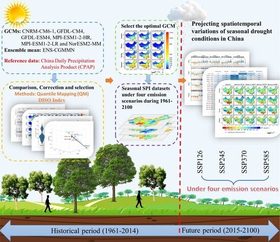
2. Materials and Methods

2.1. Study Area

China, the world’s third largest country, is distinguished by its diverse topography and terrain, as well as climate zones [52]. Mean elevations reveal that China’s terrain is generally elevated in the west and low in the east, which partially explains the spatial heterogeneity of precipitation amount in China [53] (Figure 1). According to studies, the East Asian monsoon system is China’s primary precipitation source and determines the regional distribution of precipitation [54,55]. During the summer, the EASM is the most significant precipitation mechanism, accounting for 40–50% of annual precipitation in southern China and 60–70% of annual precipitation in northern China [40,56]. Similarly, a considerable correlation is discovered between interannual variations of the East Asian Winter Monsoon (EAWM) and winter precipitation over southeastern China [57]. Xinjiang (XJ), (II) Qinghai-Tibet Plateau (QTP), (III) Northwest (NW), (IV) Northeast (NE), (V) North China (NC), (VI) Southwest (SW), and (VII) South China (SC) are the seven climatic subregions of China, according to our previous research [58]. XJ and NW have a temperate continental environment, whereas QTP and NE have a plateau alpine climate and a temperate monsoon climate, respectively. In contrast, NC, the SW, and SC are dominated by a subtropical monsoon climate. The primary abbreviations and corresponding full names involved in this study can be found in

Table A1. Primary abbreviations and corresponding full names are presented in this study.

Abbreviation	Full Name
XJ	Xinjiang
QTP	Qinghai–Tibetan Plateau
NW	Northwest
NE	Northeast
NC	Northern China
SW	Southwest
SC	Southern China
QM	quantile mapping
SPI	standardized precipitation index
CPAP	China Daily Precipitation Analysis Product
GCM	global climate models
RCP	Representative Concentration Pathway
SSP	Shared Socioeconomic Pathway
CMIP	Coupled Model Intercomparison Project
IPCC	Intergovernmental Panel on Climate Change
AR	Assessment Report
CMA	China Meteorological Administration
CC	correlation coefficient
RMSE	root-mean square error
SD	standard deviation
AE	absolute error

.

2.2. Data Utilized and Processing

2.2.1. Reference Precipitation Observations

In this investigation, the China Daily Precipitation Analysis Product (CPAP) was used as reference precipitation data to compare, evaluate, and correct the precipitation from five GCMs. CPAP is developed from 2472 meteorological stations across China based on the climatology-based Optimal Interpolation (OI) technique [59], which is produced and released by the National Meteorological Information Center (NMIC) and China Meteorological Administration (CMA), with a spatial resolution of 0.5° × 0.5°. It is worth noting that all the observations used in CPAP have undergone strict quality control (QC), including extrema detection, internal consistency check, and spatial consistency check, before applying the OI technique [60,61]. In recent years, the CPAP has been widely used in precipitation-related (e.g., drought and runoff) investigations in China [62,63,64], particularly as reference data to validate high temporal and spatial resolution satellite-based precipitation products [59,65,66]. As a result, this research used it as a benchmark for comparing precipitation measurements with GCMs from 1961–2014. Before analysis, the daily CPAP should be aggregated into monthly total precipitation by summing daily precipitation in each month of every year from 1961–2014.

2.2.2. Global Climate Model (GCM)

Compared with CMIP5, the Coupled Model Intercomparison Project Phase 6 (CMIP6) models are proven to be more capable of capturing the spatial patterns of summer precipitation across East China [40,41]. Moreover, six models, including CNRM-CM6-1, GFDL-CM4, GFDL-ESM4, MPI-ESM1-2-HR, MPI-ESM1-2-LR, and NorESM2-MM, were considered to have a better performance for most precipitation indices in CMIP6 [67]. Since GFDL-CM4 does not have a future simulation, it will not be taken into account or analyzed in this study. Therefore, for future projections, monthly precipitation datasets from 5 model simulations, including CNRM-CM6-1, GFDL-ESM4, MPI-ESM1-2-HR, MPI-ESM1-2-LR, and NorESM2-MM, were employed in this study, which were obtained in both the historical period (1961–2014) and future period (2015–2100) from the Coupled Model Intercomparison Project Phase 6 (CMIP6) archive (https://esgf-node.llnl.gov/projects/cmip6/, accessed on 13 July 2023). The five selected models consider both shared socioeconomic pathways (SSPs) and representative concentration pathways (RCPs), which are considered to make future scenarios more reasonable [68].

Moreover, the simulations from four scenarios were employed in this study, namely, SSP126, SSP245, SSP370 and SSP585, in which SSP126 represents a sustainable world with SSP1-RCP2.6 forcing at a low level of greenhouse gas emissions; SSP245 adopts a moderate world with SSP2-RCP4.5 forcing at an intermediate level of greenhouse gas emissions [69]; SSP370 is a new scenario combination, drawing the medium-to-high end of future emissions and warming [70], while SSP585 depicts a world with rapid fossil fuel evolution with SSP5-RCP8.5 forcing at a high level of greenhouse gas emissions. In the simulation (historical and future projection) procedure, ensembles of sources of uncertainty, such as uncertainties in initial conditions, are considered (e.g., r1i1p1f2 and r2i1p1f2). The details of the selected models are illustrated in

Table 1. Details of five used Global Climate Models (GCMs).

Model	Number of Ensembles					Spatial Resolution	Time Series
	Hindcast	SSP126	SSP245	SSP370	SSP585	Lat/Lon	Hindcast	Projection
CNRM-CM6-1	30	6	6	6	6	1.4 × 1.4 degree	January 1961 to December 2014	January 2015 to December 2100
GFDL-ESM4	3	1	3	1	1	1.0 × 1.25 degree
MPI-ESM1-2-HR	10	2	2	10	2	0.93 × 0.93 degree
MPI-ESM1-2-LR	31	30	30	30	30	1.86 × 1.87 degree
NorESM2-MM	3	1	2	1	1	0.9 × 1.25 degree

. The five used GCMs included 77 and 171 ensemble members for the historical (1961–2014) and future (2015–2100) periods, respectively.

Studies showed that a simple but effective method to offset the positive and negative bias of simulations is the arithmetic mean of the raw GCMs, using all ensemble members of each GCM [71,72]. Similarly, the same method was applied to obtain a new projection dataset using all five models, which is referred to as ENS-CGMMN hereafter. To uniform the spatial resolution of all GCMs and ENS-CGMMN, all of them were resampled to be 0.5 × 0.5° by using the nearest neighbor remapping algorithm from the Climate Data Operators (CDO) package, which can maintain total precipitation to a desired degree of accuracy [73] and has been employed in many related studies [74,75,76,77]. Like CPAP, the GCMs and ENS-CGMMN were also aggregated into monthly total precipitation by summing monthly precipitation in each season of every year during 1961–2100.

2.3. Methods

2.3.1. Quantile Mapping (QM) Method

The QM method has been widely employed to implement statistical transformations for correcting different global or regional climate modeling outputs [78,79,80]. Specifically, the statistical transformations involve transforming the cumulative distribution function (CDF) of the GCMs into the referenced one using a mathematical function, which can be mathematically expressed as Equation (1):

$$y=F_{ref}^{-1}\left(F_{GCM}{\displaystyle (}X{\displaystyle )}\right)$$

(1)

in which $F_{ref}^{-1}$ is the inverse of the CDF or quantile function of the reference data, X the precipitation projections of GCMs and ENS-CGMMN, and $F_{GCM}$ represents the CDF of the GCM and ENS-CGMMN simulations. It is important to highlight that the GCM or ENS-CGMMN and the reference precipitation observations for the historical period (correction period) in this study must have the same temporal and spatial resolution and the same time series.

So far, various frameworks have been proposed to form the transformation function (TF) [78], which are primarily categorized as Parametric Transformation Functions (PTF) [81,82], Distribution Derived Transformations (DIST) [83], Empirical Quantiles (QUANT) [84], Robust Empirical Quantiles (RQUANT) [85] and Smoothing Splines (SSPLIN) [86]. Among these TFs, the QUANT is proven to be a satisfying option to correct the bias of precipitation amount when it comes to the diverse topographic conditions [78]. QUANT, in contrast to PTF, is a non-parametric approach that uses empirical CDFs to estimate values for uniformly spaced quantiles of reference precipitation and GCM/ENS-CGMMN simulated precipitation [80]. Therefore, the transformation function QUANT was adopted to correct the GCM/ENS-CGMMN simulations during 1961–2100 based on the reference precipitation observations from 1961–2014. Specifically, this method makes the empirical CDF of the raw output precipitation of GCMs/ENS-CGMMN as close as possible to that of the reference precipitation observations during the historical period and then applies the established TF to the future period. The entire correction process can be depicted as Equations (2) and (3):

$$p{r}_{hist}^{QM}=ICD{F}_{ref}(CD{F}_{hist}(p{r}_{hist}))$$

(2)

$$p{r}_{fut}^{QM}=ICD{F}_{ref}(CD{F}_{hist}(p{r}_{fut}))$$

(3)

where ICDF is the corresponding inverse CDF, and pr, ref, hist and fut are precipitation, reference precipitation observations, and historical and future period, respectively; pr^QM represents the post-correction precipitation.

2.3.2. DISO Index

To compare and evaluate the performance of different GCMs/ENS-CGMMN depicting the actual precipitation, a comprehensive and sophisticated accuracy assessment method should be employed. Taylor diagram, a commonly used evaluation method, relates the “centered” root-mean-square error (RMSE), the pattern correlation coefficient (CC) and the standard deviation (SD) [87]. It shows what percentage of the RMSE can be attributed to the variance difference and what percentage may be attributed to insufficient pattern similarity [88]. However, several obvious limitations have been found as follows [89]: (1) the chosen statistical metrics must satisfy the cosine law, (2) the standard deviations in the Taylor diagram only describe the statistical characteristics of the models, not directly describing the model’s performances, and (3) it is difficult to distinguish a model’s performance when there are many simulated models, especially for models with similar performance. To overcome such issues, a sophisticated evaluation system, the DISO index, with physical mechanisms was developed by Hu et al. [89,90,91], which is extendable in terms of metrics. In light of this, the DISO index is preferable to the Taylor diagram for quantifying models’ overall performance [88]. Generally, three statistical indices, including CC, absolute error (AE), and RMSE, are used in the DISO index, which can be expressed as Equations (4)–(6):

$$CC=\frac{{\displaystyle \sum _{k=0}^n\left(S_i-\overline{S}\right)\left(R_i-\overline{R}\right)}}{\sqrt{{\displaystyle \sum _{k=0}^n{\left(S_i-\overline{S}\right)}^2}}\sqrt{{\displaystyle \sum _{k=0}^n{\left(R_i-\overline{R}\right)}^2}}}$$

(4)

$$AE=\frac{1}{n}{\displaystyle \sum _{k=0}^n\left(S_i-R_i\right)}$$

(5)

$$RMSE=\sqrt{\frac{1}{n-1}{\displaystyle \sum _{i=1}^n{\left(S_i-R_i\right)}^2}}$$

(6)

in which S and R represent simulation precipitation of GCMs/ENS-CGMMN and reference precipitation observations, respectively; $\overline{S}$ and $\overline{R}$ are the corresponding mean precipitation of S and R, respectively; and n is the size of time series. Note that before feeding data into the DISO index, the dimensional impact of AE and RMSE must be eliminated; the index may then be normalized by dividing by the absolute mean reference precipitation $\left|\overline{R}\right|$ [89]. Accordingly, the DISO index can be described as Equation (7):

$$DISO=\sqrt{{\left(r-1\right)}^2+NA{E}^2+NRMS{E}^2}$$

(7)

in which NAE and NRMSE are normalized AE and RMSE, respectively. The performance of simulations from GCMs or ENS-CGMMN depicting the reference precipitation is higher when the DISO index approaches 0 [89]. Through comparison between model-simulated precipitation and reference precipitation observations, the model with the best performance will be selected to obtain a drought index and analyze future drought conditions.

2.3.3. Standardized Precipitation Index (SPI)

Standardized Precipitation Index (SPI) expresses the actual precipitation as standardized deviation from precipitation probability distribution function [92], which has been widely used as an effective drought indicator due to its simplicity and comparability across space and time [93,94,95]. In the original SPI, the frequency distribution of precipitation was described using a two-parameter gamma probability density function (PDF) [96]. Moreover, the utilization of empirical probability can result in the derivation of a standardized index that is nonparametric in nature, thereby indicating the absence of a definite structure for the model parameters in nonparametric distributions [97]. Therefore, the empirical Gringorten distribution was employed to obtain the marginal probability of precipitation, which can be expressed as Equation (8) [98]:

$$p(x_i)=\frac{i-0.44}{n+0.12}$$

(8)

in which n and i represent the sample size and the order of the observation from the smallest, respectively, and p(x_i) is the corresponding empirical probability. Then, the SPI can be formulated as Equation (9):

$$SP{I}_i={\varphi }^{-1}(p(x_i))$$

(9)

where $\varphi$ is the standard normal distribution function. Additionally, the widely used approximate formula can be employed to standardize the percentiles [92,97,99], shown in Equation (10):

$$SP{I}_i=\left\{\begin{array}{c}-\left(t_i-\frac{C_0+C_1{t}_i+C_2{t}_i{}^2}{1+d_1{t}_i+d_2{t}_i{}^2+d_3{t}_i{}^3}\right)\begin{array}{c}\begin{array}{cc}& if\begin{array}{c}0<p\le 0.5\end{array}\end{array}\end{array}\\ +\left(t_i-\frac{C_0+C_1{t}_i+C_2{t}_i{}^2}{1+d_1{t}_i+d_2{t}_i{}^2+d_3{t}_i{}^3}\right)\begin{array}{cc}& if\begin{array}{c}0.5<p\le 1\end{array}\end{array}\end{array}\right.,$$

(10)

in which C₀, C₁, C₂, d₁, d₂ and d₃ are 2.515517, 0.802583, 0.010328, 1.432788, 0.189269 and 0.001308, respectively; and t_i can be explained by Equation (11):

$$t_i=\left\{\begin{array}{c}\sqrt{\ln \frac{1}{p{(x_i)}^2}}\begin{array}{cc} & if\begin{array}{c}0<p\le 0.5\end{array}\end{array}\\ \sqrt{\ln \frac{1}{{(1-p(x_i))}^2}}\begin{array}{cc}& if\begin{array}{c}0.5<p\le 1\end{array}\end{array}\end{array}\right.$$

(11)

Based on the above, 3-month (seasonal) time scale SPI values were calculated and analyzed during the historical (1961–2014) and future period (2015–2100) under SSP126, SSP245, SSP370 and SSP585 scenarios in this study, which, in general, is considered as agricultural drought [93]. Specifically, the seasonal time scale includes spring (March, April, and May), summer (June, July, and August), autumn (September, October, and November), and winter (December, January, and February). The 3-month SPI provides a comparison of the precipitation over a specific 3-month period (e.g., spring) with the precipitation totals from the same 3-month period for all the years included in the study period. In other words, a 3-month SPI in the spring compares the March–April–May precipitation totals for that year to those of all years. Furthermore, 3-month SPI reflects short- and medium-term moisture conditions and provides a seasonal estimation of dry and wet conditions.

In addition, the drought severity can be divided into seven levels according to the SPI values. Generally, negative and positive values indicate dry and wet periods, respectively [100]. Specifically, the SPIs greater than 2.0, 1.5 to 2.0, and 1.0 to 1.5 represent extremely, very, and moderately wet conditions, respectively, while the SPIs values less than −2.0, −2.0 to −1.5, and −1.5 to −1 are corresponding to extreme, severe, and moderate aridities [101]. In addition, conditions are considered to be close to normal when the values range from −1 to 1 [102]. The same classification scheme is also adopted in this study.

3. Results

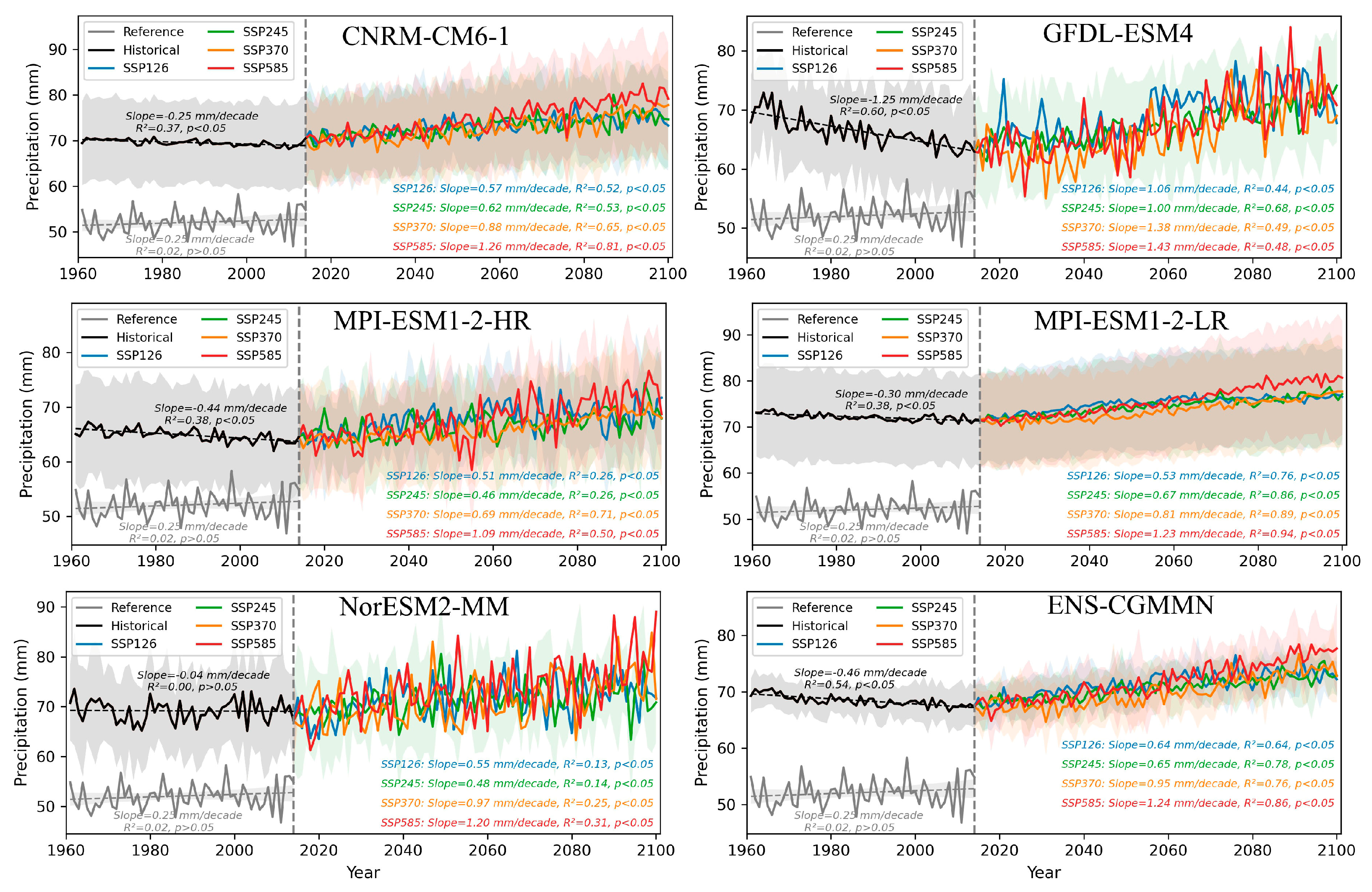
3.1. Inter-Comparisons between GCMs and Reference Precipitation

As shown in Figure 2, five GCMs and their ensemble mean ENS-CGMMN (hereafter called GCMs) are selected and employed for the inter-comparisons analysis at the temporal scale during historical and future periods. As for the first five GCMs, the curves in black, blue, green, orange, and red denote the arithmetic average of precipitation from their respective ensemble members (e.g., r1i1p1f1, r2i1p1f1), and the shadow areas represent the positive/negative standard deviations. Unlike the first five GCMs, the curves in ENS-CGMMN mean the arithmetic average of precipitation from the first five GCMs, while the shadow areas indicate the corresponding standard deviation. Apparently, all six GCMs overestimated precipitation amounts compared with reference precipitation observations during the historical period over China. Specifically, the multi-annual monthly average of precipitation during the historical period for the six models was 69.6, 66.3, 64.9, 72.1, 69.2 and 68.4 mm, respectively, while it was merely 52.1 mm for the reference precipitation observations. In this regard, the model MPI-ESM1-2-HR has the highest consistency with reference precipitation observations. Moreover, there are opposite trends in precipitation between six GCMs and reference data during the historical period. Therefore, it is unreasonable to apply precipitation simulations from GCMs before bias-corrections [103].

In terms of precipitation variations during future periods, although all six GCMs showed increasing trends in precipitation for different scenarios (i.e., SSP126, SSP245, SSP370 and SSP585), large discrepancies were found in precipitation change rates and fluctuations. The models GFDL-ESM4, MPI-ESM1-2-HR and NorESM2-MM were characterized by relatively larger fluctuations than CNRM-CM6-1, MPI-ESM1-2-LR and ENS-CGMMN. It should be noted that a higher or lower fluctuation does not necessarily suggest a better or worse performance since GCMs can introduce considerable uncertainties to their outcomes due to their coarse nominal spatial resolutions [104]. For example, sometimes GCMs-based precipitation projection may miss the extremities [104,105]. Therefore, further inter-comparisons need to be performed to comprehensively understand the performance of different GCMs.

Figure 3 shows the spatial inter-comparisons between reference precipitation and six GCMs’ precipitation at the seasonal scale during the historical period. Significant overestimations can be found in the adjacent regions of QTP and SW for the six models, where precipitation is most likely to have a large deviation in climate models, as well as in satellite and reanalysis-based precipitation products [106,107]. Specifically, in autumn, all six models showed sound performances in northerly areas of China, including XJ, NW, NE, NC and most parts of QTP, while all of them nearly failed to capture the actual spatial pattern in southerly areas (i.e., SW and SC). In the winter, the erroneous spatial precipitation patterns primarily appeared in SC and SW. However, in spring and summer, all seven subregions showed different degrees of spatial precipitation pattern errors, among which the CNRM-CM6-1, MPI-ESM1-2-LR, and NorESM2-MM resulted in comparatively greater precipitation overestimations. Therefore, GFDL-ESM4, MPI-ESM1-2-HR and ENS-CGMMN had relatively higher performances in capturing precipitation spatial patterns over China. Moreover, the performance of seasonal precipitation series from GCMs was also examined during the historical period. As shown in Figure 4, according to the median and density distributions, MPI-ESM1-2-HR presented the optimal performance among all models, compared with reference precipitation observations.

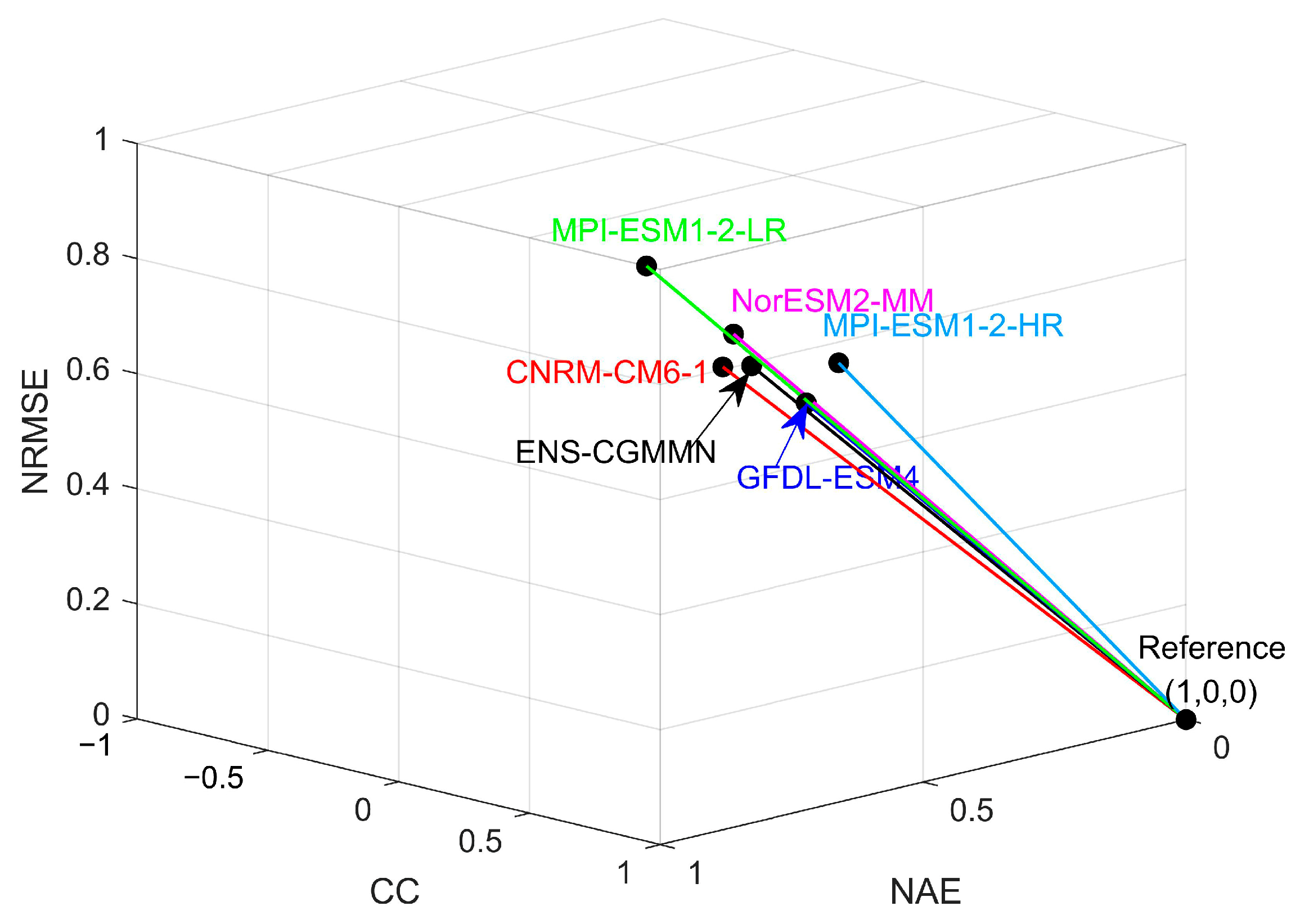
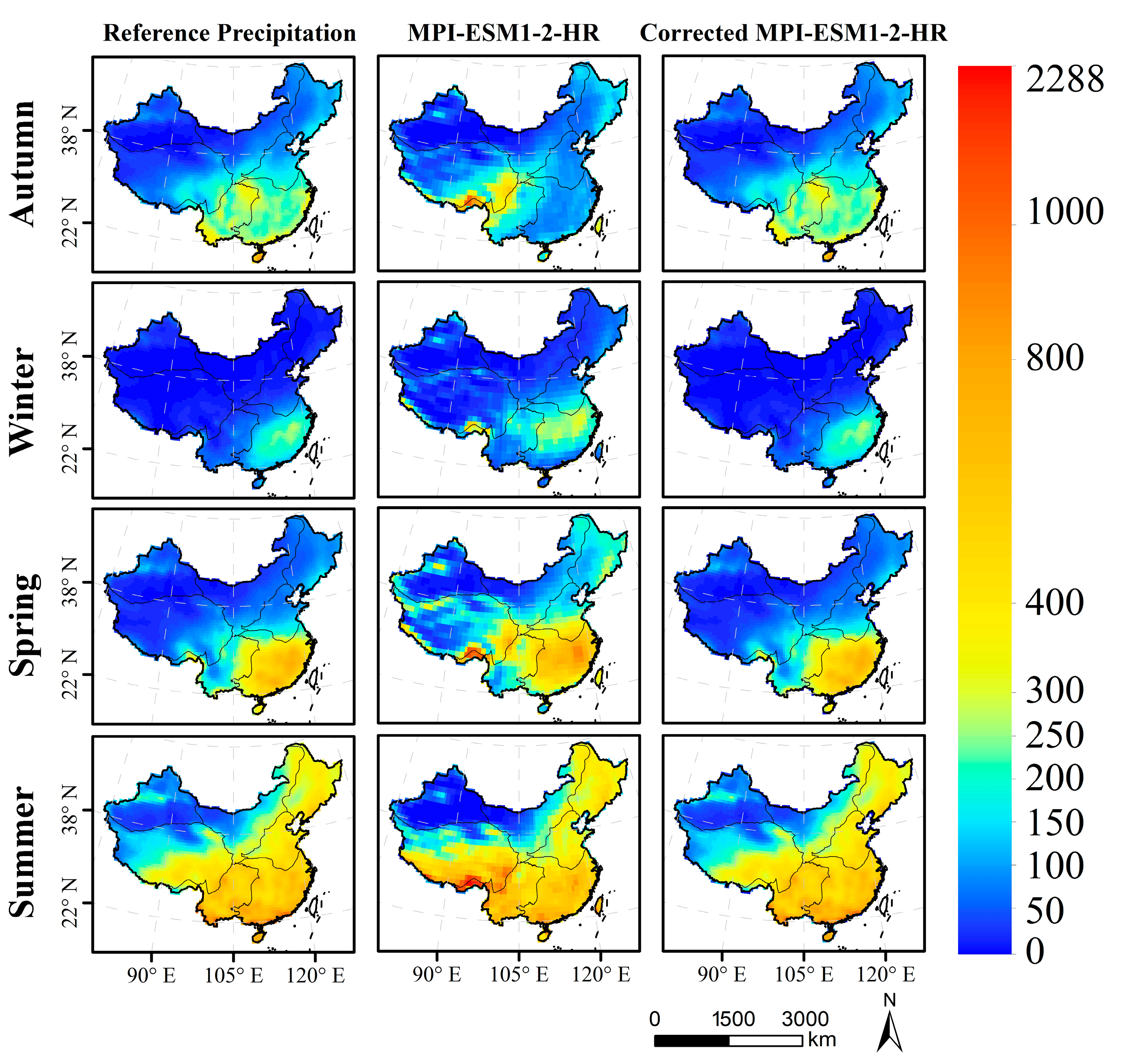
3.2. Evaluation and Correction of GCMs and ENS-CGMMN

As described in Section 2.3.2, DISO is a comprehensive and sophisticated tool in the evaluation of the overall performance of global climate models. Therefore, the seasonal performance of models in estimating precipitation was evaluated statistically using the DISO in this study. Figure 5 shows the performance of five GCMs (i.e., CNRM-CM6-1, GFDL-ESM4, MPI-ESM1-2-HR, MPI-ESM1-2-LR, and NorESM2-MM) and their ensemble average ENS-CGMMN at seasonal scale during the historical period (1961–2014) over China, compared with the reference precipitation CPAP. Different colors are used to depict the discrepancy in distances between simulations and reference precipitation observation from CPAP. The shorter distances denote the higher holistic performance of models. It is obvious that raw MPI-ESM1-2-LR has the worst performance, with the longest distance, while the GFDL-ESM4, MPI-ESM1-2-HR and ENS-CGMMN have relatively shorter distances, indicating relatively higher overall performance.

Combined with

Table 2. The statistical metrics used in 3-dimension (DISO-3) and DISO-3 index for 5 raw Global Climate Models (GCMs) and ensemble mean: CNRM-CM6-1, GFDL-ESM4, MPI-ESM1-2-HR, MPI-ESM1-2-LR, NorESM2-MM, and ENS-CGMMN.

Models	CC	AE (mm)	RMSE (mm)	DISO 1
CNRM-CM6-1	0.98	51.19	55.87	1.18
GFDL-ESM4	0.97	41.55	48.93	1.00
MPI-ESM1-2-HR	0.94	37.07	52.41	0.98
MPI-ESM1-2-LR	0.95	58.71	69.80	1.42
NorESM2-MM	0.98	49.94	59.53	1.20
ENS-CGMMN	0.97	47.69	55.03	1.13

¹ It represents the 3d DISO index, including CC, AE and RMSE.

, it can be seen that all the CCs of six models are beyond 0.94, among which the models with the highest (0.98) and the lowest CC (0.94) are CNRM-CM6-1/NorESM2-MM and MPI-ESM1-2-HR, respectively. In contrast to CC, the performance of GFDL-ESM4, MPI-ESM1-2-HR and ENS-CGMMN in AE is relatively better than other models, with values of 41.55, 37.07 and 47.69 mm, respectively. Similarly, in terms of AE, the same three models of GFDL-ESM4, MPI-ESM1-2-HR and ENS-CGMMN have better accuracy among all models, with values of 48.93, 52.41 and 55.03 mm, respectively. With a value of 0.98, the comprehensive index DISO reveals that MPI-ESM1-2-HR, and not the ENS-CGMMN, has the greatest overall performance among the six models. However, to check if the model MPI-ESM1-2-HR can still maintain the best overall performance after data correction with the QM method, the first three models GFDL-ESM4, MPI-ESM1-2-HR and ENS-CGMMN in the historical period were selected to complement the data correction with the reference precipitation observation at the monthly scale.

As shown in

Table 3. The statistical metrics used in 3-dimension (DISO-3) and DISO-3 index for two corrected Global Climate Models (GCMs) and the ensemble mean: GFDL-ESM4, MPI-ESM1-2-HR, and ENS-CGMMN.

Models	CC	AE (mm)	RMSE (mm)	DISO 1
GFDL-ESM4	0.98	0.06	20.78	0.97
MPI-ESM1-2-HR	0.98	0.02	20.87	0.97
ENS-CGMMN	0.98	−0.04	21.58	1.00

¹ It represents the 3d DISO index, including CC, AE and RMSE.

, all three statistical metrics, CC, AE and RMSE, are improved greatly at the seasonal scale after data correction, particularly for MPI-ESM1-2-HR, rising from 0.94 to 0.98. Moreover, this mode has lower AE and RMSE errors, with values of 0.02 and 20.87, respectively, which means that it has a better accuracy among the post-corrected models of GFDL-ESM4, MPI-ESM1-2-HR, and ENS-CGMMN. From the perspective of the DISO index, the same overall performance, with a value of 0.97, is shown in GFDL-ESM4 and MPI-ESM1-2-HR models. Given that the raw MPI-ESM1-2-HR has a higher nominal spatial resolution than GFDL-ESM4 (see Table 1), the former was selected to conduct further analysis in this study. To check the consistency of the spatial precipitation pattern between the post-corrected MPI-ESM1-2-HR simulations and reference precipitation observations, the spatial distribution maps of multi-year mean seasonal precipitation during the historical period for reference data, raw MPI-ESM1-2-HR, and corrected MPI-ESM1-2-HR are drawn in Figure 6. Obviously, the performance of MPI-ESM1-2-HR in depicting the actual precipitation is significantly improved in both values and spatial patterns in autumn, winter, spring and summer, especially for the exceptionally high values located in the adjacent regions of QTP and SW. Therefore, the post-corrected MPI-ESM1-2-HR can be confidently employed in calculating the SPI and associated analysis of drought conditions at a seasonal scale.

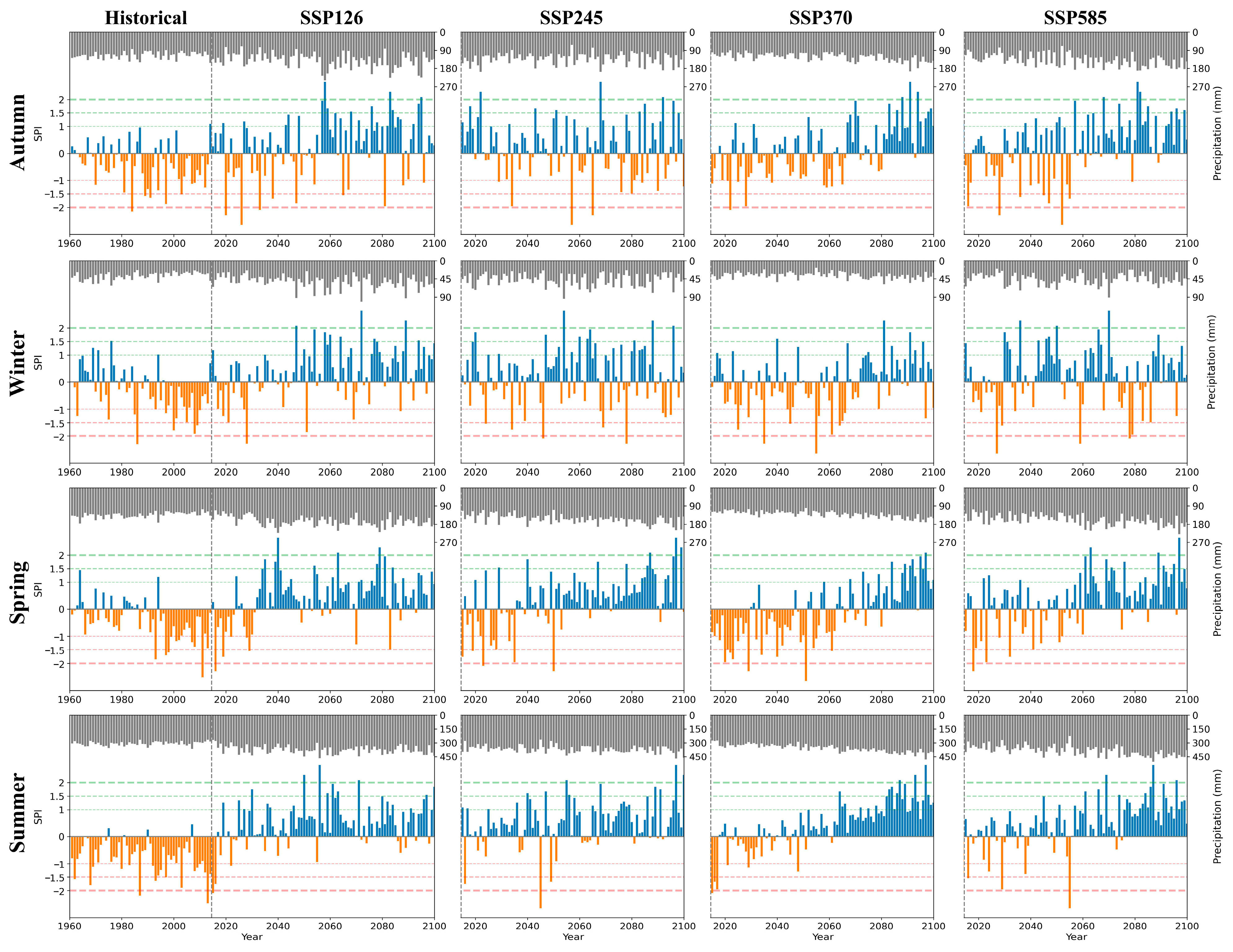
3.3. Spatiotemporal Variations of Seasonal Drought Conditions in China

Based on the monthly precipitation of post-corrected MPI-ESM1-2-HR, the seasonal SPI (3-month scale) was calculated during the historical (1961–2014) and future periods (2015–2100) over China (Figure 7). In autumn (Figure 7 1st row), the mean precipitation during the historical period was 115.56 mm, while, in the future period, these were 141.03, 131.63, 123.51 and 139.26 mm under SSP126, SSP245, SSP370 and SSP585 scenarios, respectively. It suggests that precipitation under all four scenarios would increase to varying degrees in the future compared with the historical period. Correspondingly, by reference to the SPI variations in the historical period, China will experience a significant dry-to-wet climate change under all four scenarios during 2015–2100. In particular, the mean occurrence frequencies of various drought levels during historical and future periods were determined by dividing the number of autumn occurrences of a given drought level by the number of years in the corresponding historical or future period (Figure 8). It appears that the frequency of moderate, severe, and extreme aridity in autumn has decreased, particularly severe aridity under the SSP245 and SSP370, whereas the frequency of moderate, very, and extremely moist conditions has increased significantly. When compared with the historical period, the frequencies of extremely wet and very wet conditions in the season have a comparable increase under the four emission scenarios in the future. Like extreme and very wet conditions, the frequency of moderately wet conditions increased under all scenarios, with scenario SSP370 having the least magnitude, with a value of 0.12 times/yr.

In winter (Figure 7 2nd row), the mean precipitation was 37.91 mm for the historical period, but, unlike autumn, it did not have a large increasing magnitude under the scenarios of SSP126, SSP245 and SSP585 in the future, with the mean precipitation of 52.14 mm, 47.66 mm and 46.18 mm, respectively. It is worth noting that even under the SSP370, the mean precipitation (merely 36.8mm) decreased slightly compared with the historical period. When combined with Figure 8, the features of dry to wet can also be seen clearly in the winter under SSP126, SSP245 and SSP585, except SSP370. Specifically, moderate and extreme aridity have a very similar frequency variation under four scenarios. However, there are distinct discrepancies in extreme, very, moderately wet and severe aridity conditions between SSP370 and other scenarios, under which there is no significant increase in wet condition frequency and no significant decrease in aridity frequency.

In spring (Figure 7 3rd row), the mean precipitation under SSP126, SSP245, SSP370 and SSP585 was 165.11 mm, 154.65 mm, 131.23 mm and 159.15 mm, respectively, which were larger than the mean precipitation of 134.58 mm in the historical period, except for SSP370. Comparing the historical periods, all four future scenarios show a trend of change from dry to wet. However, specifically, among these four scenarios, the frequencies of moderate, severe, and extreme aridity under the SSP370 only slightly decrease or increase, and the frequencies of moderately, very, and extremely wet conditions also increase significantly less (Figure 8).

In summer (Figure 7 4th row), precipitation is most abundant during the whole year. The average precipitation during this season in the historical period is 308.49 mm, while in the future, under the four scenarios, it shows different degrees of increase, with the largest increase being 386.70 mm under SSP585. In terms of SPI, compared to the historical period, the future scenarios show a clear change from dry to wet. Combined with Figure 8, it can be found that the frequencies of moderately, very, and extremely wet conditions show an identical increase in summer, while the frequencies of moderate, severe and extreme aridity all show a decreasing trend but with some fluctuations. Specifically, the decrease in the frequency of moderate aridity was slightly smaller under SSP370 than in other scenarios.

To investigate the spatial variation characteristics of SPI, the change trends and associated significances in China were obtained and mapped in Figure 9. In autumn (Figure 9 1st row), SPI showed a significant decreasing trend, namely tending to dry conditions, in SW and the northwest of SC during the historical phase, while the other subdivisions showed largely insignificant variations, although most of them showed a wet trend. In comparison with the historical period, the decreasing rate of SPI becomes smaller in the SW under the four future scenarios, while QTP NW shows a significant increasing trend. For the southern part of SC, the SPI shows a significant increasing trend under the SSP245 scenario and is more pronounced than the other three scenarios.

In winter (Figure 9 2nd row), SPI showed an overall decreasing trend in the southern subregions and an increasing trend in the northern subregions of China during the historical period. Specifically, a significant decreasing trend was observed in SW, SC, southern QTP and southeastern NE, while a significant decreasing trend was found in northern XJ, southern NW and west-central NC. Compared with the historical period, the aridity of the southern subregions decreased to different degrees under the four future scenarios, as evidenced by a decrease in the significant area and change rates and even a change from dry to wet conditions in the southern SW, southern QTP and northwestern SC under the SSP245 scenario. In contrast, the wetness of the northern subregions increased, as revealed by a significant increase in the significant area. However, the change rate varies significantly among scenarios, with the change rate increasing significantly in XJ, NW, NE, and NC under the SSP126 scenario, followed by the SSP585 scenario, while the change rate in these areas increases under the SSP245 and SSP370 scenarios to a lesser extent than in the historical period, except for the NE.

In spring (Figure 9 3rd row), SPI showed a significant increasing trend in the west-central and east-central parts of QTP and the northeastern part of NW during the historical period. However, SW and the central and southern parts of SC showed a significant decreasing trend. Compared with the historical period, the sub-regions located in the northern subregions of China generally show an increasing trend of wetness under the four future climate scenarios, which is mainly reflected in the expansion of the significant area of wet areas, especially under the SSP126 scenario. In this scenario, the SPI of QTP, NC, NW, NE, and northern XJ increases significantly and exceeds the other three climate scenarios in terms of increase rate and significant area. Meanwhile, the southern subregions of China show a decreasing trend in aridity, with particularly significant changes under the SSP126 and SSP245 scenarios.

In summer, the variations of SPI in the historical period differ significantly from the other seasons in terms of spatial patterns. Except for the increasing trend in the central-north and central-west parts of the QTP, the other regions of China generally show a decreasing trend, especially in the XJ, where this is the exact opposite of the other seasons. Comparing the historical period, the area with a significant tendency of dryness in XJ further expands in the future under the four scenarios, especially in the SSP245 scenario, while the area with a significant tendency of wetness increases in NE, NC, and SC. It should be noted that the area with a wet trend in the central part of the NW increases significantly under the SSP245 scenario.

4. Discussion

4.1. Uncertainty in the Standardized Precipitation Index

The Standardized Precipitation Index (SPI) is widely recognized in drought monitoring and research on a global scale because of its suitability for spatial and seasonal comparisons, flexibility, lower computational demands in comparison to other indices, and ease of application [108]. Furthermore, although the SPI is solely based on precipitation data, it coincides with the fact that precipitation remains a key factor influencing drought in many regions [29,109,110]. Therefore, SPI is considered to be a well-tested and generally accepted index for the drought assessment [25,111], which is the main reason for using SPI in this study. However, there may be some ambiguity with the use of SPI compared to other drought indices, such as the Standardized Precipitation Evapotranspiration Index (SPEI), in measuring drought in climatically complex regions due to the limitations of SPI based on precipitation data alone [108,112]. Specifically, SPI relies only on precipitation data and does not consider other important meteorological variables, such as evapotranspiration, while it is closely related to soil moisture and vegetation conditions and has important impacts on drought [113,114,115]. It is possible that SPI underestimates the effects of climate change on drought in some cases. For example, drought conditions may intensify in the presence of increased evapotranspiration due to increasing temperatures, even if precipitation remains constant [116].

That is, in fact, what transpired. Global warming has led to an overall increase in global land surface evapotranspiration since 1982 [117]. Su et al. [118] revealed that annual mean evapotranspiration in China has increased significantly during the period of 1980–2015, and the major regime shift occurred around 1998, with an ensemble of six reanalyzes and a complementary-relationship-based evapotranspiration dataset. Pan et al. [119] utilized four remote-sensing-based physical models, two machine-learning algorithms and 14 land surface models to analyze the spatiotemporal variations in global terrestrial evapotranspiration and concluded that both the ensembles of remote-sensing-based physical models and machine-learning algorithms suggested increasing trends in global terrestrial evapotranspiration during the period of 1982–2011. Ma et al. [120] investigated the spatiotemporal features of actual evapotranspiration in sandy areas in northern China under global warming scenarios of 1.5 °C and 2.0 °C and found that the actual evapotranspiration under only the representative concentration pathway 2.6 (RCP2.6) emission scenario increased towards a plateau and significantly increased in the other three emission scenarios (p < 0.01) under global warming of 1.5 °C and 2.0 °C. Therefore, in this case, SPI may not accurately reveal the actual status of drought under future emission scenarios.

However, it is worth noting that the use of SPI may also be a good choice when data are limited or when the main focus is on the effect of precipitation on drought, such as in this study where the focus is on the calibration and validation of high-performance precipitation data and not on evapotranspiration. However, a drought index with more thorough considerations (e.g., SPEI) may be preferable in circumstances when data are available and multiple climatic elements, such as precipitation and evapotranspiration, need to be taken into account [121].

4.2. Reasonality of the Main Findings in this Study

In this study, the authors obtained a series of significant findings regarding the performance of global climate models (GCMs) in projecting precipitation and analyzing drought characteristics in China. This section will discuss the reasonability of the main findings. First, five selected GCMs with better performance [67], including CNRM-CM6-1, GFDL-ESM4, MPI-ESM1-2-HR, MPI-ESM1-2-LR, NorESM2-MM, and their ensemble average ENS-CGMMN generally still overestimate precipitation in China during the historical period, indicating that existing GCMs still have some uncertainties in projecting precipitation, especially in countries and regions with complex topographic and seasonal variations [122,123,124]. Nevertheless, the performance evaluation of the selected models in this study revealed that there are still some raw GCMs that are acceptable in depicting the spatial patterns of precipitation in China (e.g., GFDL-ESM4 and MPI-ESM1-2-HR). Moreover, the GCMs (e.g., MPI-ESM1-2-HR) significantly improved the reliability of precipitation projection results after correcting the GCMs by the quantile mapping (QM) method. This implies that when using climate models for climate change studies, the evaluation of model performance in advance and the use of appropriate bias correction methods may significantly improve the reliability of the results and make the conclusions more reliable [125,126,127].

Second, the authors found that the best one of the selected GCMs and their ensemble mean ENS-CGMMN in depicting precipitation is MPI-ESM1-2-HR and not the ENS-CGMMN. A possible reason can be that the accuracy of multi-model ensemble mean was influenced mainly by the low-skill GCMs, such as MPI-ESM1-2-LR, which was also confirmed by Aadhar and Mishra [43] in their study of CMIP6 multi-model ensemble projection of drought in South Asia. They reported that the ensemble mean of GCMs is profoundly affected by the poor-performing models that project an unrealistic increase in the summer monsoon precipitation under the warming climate [128]. Specifically, the poor representation of atmospheric processes and feedback in the GCMs affects convection sensitivity and increased warming in the GCMs results in a strong thermodynamic process [129], which conversely causes an increase in precipitation under the warming climate [129,130]. Consequently, a large increase in the convective precipitation in the poor-performing GCMs might be associated with the poor representation of land-atmospheric feedback and convection in the GCMs of the CMIP6 [42,43,131].

In the future period of 2015–2100, the authors found that China’s climate will generally show an arid to wet transition under four different scenarios, including SSP126, SSP245, SSP370 and SSP585. Moreover, a general increase will occur in wetness in the northern subregions of China in the future. Meanwhile, the dryness in the southern subregions will decrease. These findings highlight the potential for diverse impacts of climate change across seasons and regions, which is critical for developing adaptive strategies and resource management measures. Importantly, they were, to some extent, consistent with the conclusion from several published literature, such as Wang and Chen [132], revealed that a remarkable increase is found over most areas of China except the southwest, ranging from approximately 2 to 20%, and the projected precipitation changes are highly robust in northern China but inconsistent in southern China during 2010–2099 under RCP4.5 and RCP8.5 scenarios. Xu et al. [133] argued that future changes in precipitation extremes are projected to clearly increase across China over the coming century under the SSP245 and SSP585 scenarios, while the dry condition index of consecutive dry days exhibits a decreasing tendency in the future, which all imply that the dry conditions induced by precipitation anomalies will be mitigated. This suggests that China may face increased precipitation as global climate change evolves, which could have important impacts on its socio-economic and ecological systems [134].

Overall, uncertainties do likely exist in the present study. However, the results of this study can provide strong support for future climate change and drought research, help improve the accuracy of future climate predictions, and provide a reference for drought risk management and policy development.

5. Conclusions

The main findings in the present study can be shown as follows:

Five selected global climate models (GCMs), including CNRM-CM6-1, GFDL-ESM4, MPI-ESM1-2-HR, MPI-ESM1-2-LR, NorESM2-MM, and their ensemble mean ENS-CGMMN all overestimate precipitation compared to the reference precipitation observations for the historical period in China. Among them, the MPI-ESM1-2-HR model (and not the ENS-CGMMN) has the highest agreement with the reference precipitation observation. The different GCMs differ in projecting precipitation trends and fluctuations in the future period but generally show an increasing precipitation trend.

The quantile mapping (QM) method can effectively improve the projected performance of GCMs and enhance the accuracy of precipitation data at seasonal scales. The post-corrected MPI-ESM1-2-HR model in depicting actual precipitation improves significantly in numerical and spatial patterns in all seasons, especially in the exceptional high values located in the adjacent regions of the Qinghai-Tibet Plateau (QTP) and Southwest (SW). Therefore, at the seasonal scale, the calibrated MPI-ESM1-2-HR can be confidently used to calculate the standardized precipitation index (SPI) and related seasonal drought condition analysis, providing powerful support for future climate change and drought studies.

In the future period (2015–2100), the climate of China will shift from dry to wet in general, and this change is reflected in four different scenarios (SSP126, SSP245, SSP370, and SSP585). Specifically, China has a clear trend from dry to wet in the autumn and summer. At the same time, the frequency of wetness events in China under the SSP370 scenario varies less in winter and spring than in the other scenarios. Spatially, in autumn, winter, and spring, the wetness will generally increase in China’s northern subregions, including QTP, Xinjiang (XJ), Northwest (NW), Northeast (NE), and North China (NC). Meanwhile, the dryness will decrease in the southern subregions, including SW and South China (SC). Unlike those three seasons, XJ has a significant trend toward aridity, especially in the SSP245 scenario, while NE, NC, and SC show a significant trend toward wetness in summer. Although overall characteristics were given above, significant differences were observed across seasons and subregions under the four future climate scenarios.

References

1. Otkin, J.A.; Svoboda, M.; Hunt, E.D.; Ford, T.W.; Anderson, M.C.; Hain, C.; Basara, J.B. Flash Droughts: A Review and Assessment of the Challenges Imposed by Rapid-Onset Droughts in the United States. Bull. Am. Meteorol. Soc. 2018, 99, 911–919. [Google Scholar] [CrossRef]
2. Jia, H.; Chen, F.; Zhang, C.; Dong, J.; Du, E.; Wang, L. High emissions could increase the future risk of maize drought in China by 60–70%. Sci. Total Environ. 2022, 852, 158474. [Google Scholar] [CrossRef] [PubMed]
3. FAO. The Impact of Natural Hazards and Disasters on Agriculture and Food Security and Nutrition: A Call for Action to Build Resilient Livelihoods; Food and Agriculture Organization of the United Nations: Rome, Italy, 2015. [Google Scholar]
4. Su, B.; Huang, J.; Fischer, T.; Wang, Y.; Kundzewicz, Z.W.; Zhai, J.; Sun, H.; Wang, A.; Zeng, X.; Wang, G.; et al. Drought losses in China might double between the 1.5 °C and 2.0 °C warming. Proc. Natl. Acad. Sci. USA 2018, 115, 10600–10605. [Google Scholar] [CrossRef]
5. Yu, M.; Li, Q.; Hayes, M.J.; Svoboda, M.D.; Heim, R.R. Are droughts becoming more frequent or severe in China based on the standardized precipitation evapotranspiration index: 1951–2010? Int. J. Climatol. 2014, 34, 545–558. [Google Scholar] [CrossRef]
6. Bose, A.K.; Gessler, A.; Bolte, A.; Bottero, A.; Buras, A.; Cailleret, M.; Camarero, J.J.; Haeni, M.; Hereş, A.M.; Hevia, A. Growth and resilience responses of Scots pine to extreme droughts across Europe depend on predrought growth conditions. Glob. Chang. Biol. 2020, 26, 4521–4537. [Google Scholar] [CrossRef]
7. Field, C.B.; Barros, V.; Stocker, T.F.; Dahe, Q. Managing the Risks of Extreme Events and Disasters to Advance Climate Change Adaptation: Special Report of the Intergovernmental Panel on Climate Change; Cambridge University Press: Cambridge, UK, 2012. [Google Scholar]
8. Da Rocha Júnior, R.L.; dos Santos Silva, F.D.; Costa, R.L.; Gomes, H.B.; Pinto, D.D.C.; Herdies, D.L. Bivariate Assessment of Drought Return Periods and Frequency in Brazilian Northeast Using Joint Distribution by Copula Method. Geosciences 2020, 10, 135. [Google Scholar] [CrossRef]
9. Huang, J.; Yu, H.; Guan, X.; Wang, G.; Guo, R. Accelerated dryland expansion under climate change. Nat. Clim. Chang. 2016, 6, 166–171. [Google Scholar] [CrossRef]
10. Zhang, Q.; Yao, Y.; Li, Y.; Huang, J.; Ma, Z.; Wang, Z.; Wang, S.; Wang, Y.; Zhang, Y. Progress and prospect on the study of causes and variation regularity of droughts in China. Acta Meteor. Sin. 2020, 78, 500–521. [Google Scholar] [CrossRef]
11. Yin, J.; Guo, S.; Yang, Y.; Chen, J.; Gu, L.; Wang, J.; He, S.; Wu, B.; Xiong, J. Projection of droughts and their socioeconomic exposures based on terrestrial water storage anomaly over China. Sci. China Earth Sci. 2022, 65, 1772–1787. [Google Scholar] [CrossRef]
12. Kogan, F.N. Global drought watch from space. Bull. Am. Meteorol. Soc. 1997, 78, 621–636. [Google Scholar] [CrossRef]
13. Liu, Y.; You, M.; Zhu, J.; Wang, F.; Ran, R. Integrated risk assessment for agricultural drought and flood disasters based on entropy information diffusion theory in the middle and lower reaches of the Yangtze River, China. Int. J. Disaster Risk Reduct. 2019, 38, 101194. [Google Scholar] [CrossRef]
14. Dong, Z.; Zhang, J.; Tong, Z.; Han, A.; Zhi, F. Ecological security assessment of Xilingol grassland in China using DPSIRM model. Ecol. Indic. 2022, 143, 109336. [Google Scholar] [CrossRef]
15. Ren, Y.; Liu, J.; Shalamzari, M.J.; Arshad, A.; Liu, S.; Liu, T.; Tao, H. Monitoring Recent Changes in Drought and Wetness in the Source Region of the Yellow River Basin, China. Water 2022, 14, 861. [Google Scholar] [CrossRef]
16. Grigorieva, E.A.; Livenets, A.S. Risks to the Health of Russian Population from Floods and Droughts in 2010–2020: A Scoping Review. Climate 2022, 10, 37. [Google Scholar] [CrossRef]
17. Zargar, A.; Sadiq, R.; Naser, B.; Khan, F.I. A review of drought indices. Environ. Rev. 2011, 19, 333–349. [Google Scholar] [CrossRef]
18. Odongo, R.A.; De Moel, H.; Van Loon, A.F. Propagation from meteorological to hydrological drought in the Horn of Africa using both standardized and threshold-based indices. Nat. Hazards Earth Syst. Sci. 2023, 23, 2365–2386. [Google Scholar] [CrossRef]
19. Sepulcre-Canto, G.; Horion, S.; Singleton, A.; Carrao, H.; Vogt, J. Development of a Combined Drought Indicator to detect agricultural drought in Europe. Nat. Hazards Earth Syst. Sci. 2012, 12, 3519–3531. [Google Scholar] [CrossRef]
20. Wu, H.; Hayes, M.J.; Weiss, A.; Hu, Q. An evaluation of the Standardized Precipitation Index, the China-Z Index and the statistical Z-Score. Int. J. Climatol. 2001, 21, 745–758. [Google Scholar] [CrossRef]
21. Ju, X.; Yang, X.; Chen, L.; Wang, Y. Research on determination of station indexes and division of regional flood/drought grades in China. J. Appl. Meteorol. 1997, 8, 26–33. [Google Scholar]
22. Byun, H.-R.; Wilhite, D.A. Daily quantification of drought severity and duration. J. Clim. 1996, 5, 1181–1201. [Google Scholar]
23. Hao, Z.; AghaKouchak, A. A Nonparametric Multivariate Multi-Index Drought Monitoring Framework. J. Hydrometeorol. 2014, 15, 89–101. [Google Scholar] [CrossRef]
24. Hao, Z.; AghaKouchak, A. Multivariate standardized drought index: A parametric multi-index model. Adv. Water Resour. 2013, 57, 12–18. [Google Scholar] [CrossRef]
25. Vicente-Serrano, S.M.; Beguería, S.; López-Moreno, J.I. A Multiscalar Drought Index Sensitive to Global Warming: The Standardized Precipitation Evapotranspiration Index. J. Clim. 2010, 23, 1696–1718. [Google Scholar] [CrossRef]
26. Palmer, W.C. Meteorological Drought; US Department of Commerce, Weather Bureau: Washington, DC, USA, 1965; Volume 30.
27. McKee, T.B.; Doesken, N.J.; Kleist, J. The relationship of drought frequency and duration to time scales. In Proceedings of the 8th Conference on Applied Climatology, Anaheim, CA, USA, 17–22 January 1993; pp. 179–183. [Google Scholar]
28. Blain, G.C.; da Rocha Sobierajski, G.; Weight, E.; Martins, L.L.; Xavier, A.C.F. Improving the interpretation of standardized precipitation index estimates to capture drought characteristics in changing climate conditions. Int. J. Climatol. 2022, 42, 5586–5608. [Google Scholar] [CrossRef]
29. Liu, C.; Yang, C.; Yang, Q.; Wang, J. Spatiotemporal drought analysis by the standardized precipitation index (SPI) and standardized precipitation evapotranspiration index (SPEI) in Sichuan Province, China. Sci. Rep. 2021, 11, 1280. [Google Scholar] [CrossRef]
30. Fung, K.; Huang, Y.; Koo, C. Assessing drought conditions through temporal pattern, spatial characteristic and operational accuracy indicated by SPI and SPEI: Case analysis for Peninsular Malaysia. Nat. Hazards 2020, 103, 2071–2101. [Google Scholar] [CrossRef]
31. Adisa, O.M.; Masinde, M.; Botai, J.O. Assessment of the dissimilarities of EDI and SPI measures for drought determination in South Africa. Water 2021, 13, 82. [Google Scholar] [CrossRef]
32. Elbeltagi, A.; Pande, C.B.; Kumar, M.; Tolche, A.D.; Singh, S.K.; Kumar, A.; Vishwakarma, D.K. Prediction of meteorological drought and standardized precipitation index based on the random forest (RF), random tree (RT), and Gaussian process regression (GPR) models. Environ. Sci. Pollut. Res. 2023, 30, 43183–43202. [Google Scholar] [CrossRef] [PubMed]
33. Zuo, D.-D.; Hou, W.; Zhang, Q.; Yan, P.-C. Sensitivity analysis of standardized precipitation index to climate state selection in China. Adv. Clim. Chang. Res. 2022, 13, 42–50. [Google Scholar] [CrossRef]
34. Ridder, N.N.; Pitman, A.J.; Ukkola, A.M. Do CMIP6 climate models simulate global or regional compound events skillfully? Geophys. Res. Lett. 2021, 48, e2020GL091152. [Google Scholar] [CrossRef]
35. Grose, M.R.; Narsey, S.; Delage, F.P.; Dowdy, A.J.; Bador, M.; Boschat, G.; Chung, C.; Kajtar, J.B.; Rauniyar, S.; Freund, M.B.; et al. Insights From CMIP6 for Australia′s Future Climate. Earth′s Future 2020, 8, e2019EF001469. [Google Scholar] [CrossRef]
36. Almazroui, M.; Islam, M.N.; Saeed, F.; Saeed, S.; Ismail, M.; Ehsan, M.A.; Diallo, I.; O’Brien, E.; Ashfaq, M.; Martínez-Castro, D.; et al. Projected Changes in Temperature and Precipitation Over the United States, Central America, and the Caribbean in CMIP6 GCMs. Earth Syst. Environ. 2021, 5, 1–24. [Google Scholar] [CrossRef]
37. Meinshausen, M.; Nicholls, Z.R.; Lewis, J.; Gidden, M.J.; Vogel, E.; Freund, M.; Beyerle, U.; Gessner, C.; Nauels, A.; Bauer, N. The shared socio-economic pathway (SSP) greenhouse gas concentrations and their extensions to 2500. Geosci. Model Dev. 2020, 13, 3571–3605. [Google Scholar] [CrossRef]
38. Qing, Y.; Wang, S.; Zhang, B.; Wang, Y. Ultra-high resolution regional climate projections for assessing changes in hydrological extremes and underlying uncertainties. Clim. Dyn. 2020, 55, 2031–2051. [Google Scholar] [CrossRef]
39. Zhu, H.; Jiang, Z.; Li, J.; Li, W.; Sun, C.; Li, L. Does CMIP6 Inspire More Confidence in Simulating Climate Extremes over China? Adv. Atmos. Sci. 2020, 37, 1119–1132. [Google Scholar] [CrossRef]
40. Xin, X.; Wu, T.; Zhang, J.; Yao, J.; Fang, Y. Comparison of CMIP6 and CMIP5 simulations of precipitation in China and the East Asian summer monsoon. Int. J. Climatol. 2020, 40, 6423–6440. [Google Scholar] [CrossRef]
41. Su, B.; Huang, J.; Mondal, S.K.; Zhai, J.; Wang, Y.; Wen, S.; Gao, M.; Lv, Y.; Jiang, S.; Jiang, T.; et al. Insight from CMIP6 SSP-RCP scenarios for future drought characteristics in China. Atmos. Res. 2021, 250, 105375. [Google Scholar] [CrossRef]
42. Sabeerali, C.; Rao, S.A.; Dhakate, A.; Salunke, K.; Goswami, B. Why ensemble mean projection of south Asian monsoon rainfall by CMIP5 models is not reliable? Clim. Dyn. 2015, 45, 161–174. [Google Scholar] [CrossRef]
43. Aadhar, S.; Mishra, V. On the Projected Decline in Droughts Over South Asia in CMIP6 Multimodel Ensemble. J. Geophys. Res. Atmos. 2020, 125, e2020JD033587. [Google Scholar] [CrossRef]
44. Yazdandoost, F.; Moradian, S.; Izadi, A.; Aghakouchak, A. Evaluation of CMIP6 precipitation simulations across different climatic zones: Uncertainty and model intercomparison. Atmos. Res. 2021, 250, 105369. [Google Scholar] [CrossRef]
45. Abdulai, P.J.; Chung, E.-S. Uncertainty Assessment in Drought Severities for the Cheongmicheon Watershed Using Multiple GCMs and the Reliability Ensemble Averaging Method. Sustainability 2019, 11, 4283. [Google Scholar] [CrossRef]
46. Alamgir, M.; Khan, N.; Shahid, S.; Yaseen, Z.M.; Dewan, A.; Hassan, Q.; Rasheed, B. Evaluating severity–area–frequency (SAF) of seasonal droughts in Bangladesh under climate change scenarios. Stoch. Environ. Res. Risk Assess. 2020, 34, 447–464. [Google Scholar] [CrossRef]
47. Ueda, H.; Iwai, A.; Kuwako, K.; Hori, M.E. Impact of anthropogenic forcing on the Asian summer monsoon as simulated by eight GCMs. Geophys. Res. Lett. 2006, 33, L06703. [Google Scholar] [CrossRef]
48. Wilhite, D.A.; Sivakumar, M.V.; Pulwarty, R. Managing drought risk in a changing climate: The role of national drought policy. Weather. Clim. Extrem. 2014, 3, 4–13. [Google Scholar] [CrossRef]
49. Zou, X.; Zhai, P.; Zhang, Q. Variations in droughts over China: 1951–2003. Geophys. Res. Lett. 2005, 32, L04707. [Google Scholar] [CrossRef]
50. Nam, W.-H.; Hayes, M.J.; Svoboda, M.D.; Tadesse, T.; Wilhite, D.A. Drought hazard assessment in the context of climate change for South Korea. Agric. Water Manag. 2015, 160, 106–117. [Google Scholar] [CrossRef]
51. Haro, D.; Solera, A.; Paredes, J.; Andreu, J. Methodology for drought risk assessment in within-year regulated reservoir systems. Application to the Orbigo River system (Spain). Water Resour. Manag. 2014, 28, 3801–3814. [Google Scholar] [CrossRef]
52. Wang, Z.; Li, J.; Lai, C.; Zeng, Z.; Zhong, R.; Chen, X.; Zhou, X.; Wang, M. Does drought in China show a significant decreasing trend from 1961 to 2009? Sci. Total Environ. 2017, 579, 314–324. [Google Scholar] [CrossRef]
53. Zhai, Y.; Guo, Y.; Zhou, J.; Guo, N.; Wang, J.; Teng, Y. The spatio-temporal variability of annual precipitation and its local impact factors during 1724–2010 in Beijing, China. Hydrol. Process. 2014, 28, 2192–2201. [Google Scholar] [CrossRef]
54. Qian, W.; Kang, H.-S.; Lee, D.-K. Distribution of seasonal rainfall in the East Asian monsoon region. Theor. Appl. Climatol. 2002, 73, 151–168. [Google Scholar] [CrossRef]
55. Wu, Z.-Y.; Lu, G.-H.; Wen, L.; Lin, C. Reconstructing and analyzing China’s fifty-nine year (1951–2009) drought history using hydrological model simulation. Hydrol. Earth Syst. Sci. 2011, 15, 2881–2894. [Google Scholar] [CrossRef]
56. Lei, Y.; Hoskins, B.; Slingo, J. Exploring the Interplay between Natural Decadal Variability and Anthropogenic Climate Change in Summer Rainfall over China. Part I: Observational Evidence. J. Clim. 2011, 24, 4584–4599. [Google Scholar] [CrossRef]
57. Zhou, L.-T. Impact of East Asian winter monsoon on rainfall over southeastern China and its dynamical process. Int. J. Climatol. 2011, 31, 677–686. [Google Scholar] [CrossRef]
58. Liu, J.; Ren, Y.; Tao, H.; Shalamzari, M.J. Spatial and Temporal Variation Characteristics of Heatwaves in Recent Decades over China. Remote Sens. 2021, 13, 3824. [Google Scholar] [CrossRef]
59. Chen, Z.; Qin, Y.; Shen, Y.; Zhang, S. Evaluation of Global Satellite Mapping of Precipitation Project Daily Precipitation Estimates over the Chinese Mainland. Adv. Meteorol. 2016, 2016, 9365294. [Google Scholar] [CrossRef]
60. Liu, J.; Zhang, W.; Liu, T.; Li, Q. Runoff Dynamics and Associated Multi-Scale Responses to Climate Changes in the Middle Reach of the Yarlung Zangbo River Basin, China. Water 2018, 10, 295. [Google Scholar] [CrossRef]
61. Shen, Y.; Xiong, A.; Wang, Y.; Xie, P. Performance of high-resolution satellite precipitation products over China. J. Geophys. Res. Atmos. 2010, 115, D02114. [Google Scholar] [CrossRef]
62. Liu, J.; Zhang, W. Climate Changes and Associated Multiscale Impacts on Watershed Discharge over the Upper Reach of Yarlung Zangbo River Basin, China. Adv. Meteorol. 2018, 2018, 4851645. [Google Scholar] [CrossRef]
63. Li, C.; Tang, G.; Hong, Y. Cross-evaluation of ground-based, multi-satellite and reanalysis precipitation products: Applicability of the Triple Collocation method across Mainland China. J. Hydrol. 2018, 562, 71–83. [Google Scholar] [CrossRef]
64. Zhong, R.; Chen, X.; Lai, C.; Wang, Z.; Lian, Y.; Yu, H.; Wu, X. Drought monitoring utility of satellite-based precipitation products across mainland China. J. Hydrol. 2019, 568, 343–359. [Google Scholar] [CrossRef]
65. Wei, L.; Jiang, S.; Ren, L.; Wang, M.; Zhang, L.; Liu, Y.; Yuan, F.; Yang, X. Evaluation of seventeen satellite-, reanalysis-, and gauge-based precipitation products for drought monitoring across mainland China. Atmos. Res. 2021, 263, 105813. [Google Scholar] [CrossRef]
66. Tang, G.; Clark, M.P.; Papalexiou, S.M.; Ma, Z.; Hong, Y. Have satellite precipitation products improved over last two decades? A comprehensive comparison of GPM IMERG with nine satellite and reanalysis datasets. Remote Sens. Environ. 2020, 240, 111697. [Google Scholar] [CrossRef]
67. Zhu, H.; Jiang, Z.; Li, L. Projection of climate extremes in China, an incremental exercise from CMIP5 to CMIP6. Sci. Bull. 2021, 66, 2528–2537. [Google Scholar] [CrossRef] [PubMed]
68. Change, N.C. The CMIP6 landscape. Clim. Chang. 2019, 9, 727. [Google Scholar]
69. Li, S.-Y.; Miao, L.-J.; Jiang, Z.-H.; Wang, G.-J.; Gnyawali, K.R.; Zhang, J.; Zhang, H.; Fang, K.; He, Y.; Li, C. Projected drought conditions in Northwest China with CMIP6 models under combined SSPs and RCPs for 2015–2099. Adv. Clim. Chang. Res. 2020, 11, 210–217. [Google Scholar] [CrossRef]
70. O′Neill, B.C.; Tebaldi, C.; Van Vuuren, D.P.; Eyring, V.; Friedlingstein, P.; Hurtt, G.; Knutti, R.; Kriegler, E.; Lamarque, J.-F.; Lowe, J. The scenario model intercomparison project (ScenarioMIP) for CMIP6. Geosci. Model Dev. 2016, 9, 3461–3482. [Google Scholar] [CrossRef]
71. Dey, A.; Sahoo, D.P.; Kumar, R.; Remesan, R. A multimodel ensemble machine learning approach for CMIP6 climate model projections in an Indian River basin. Int. J. Climatol. 2022, 42, 9215–9236. [Google Scholar] [CrossRef]
72. Baghanian, S.; Alizadeh, M.J. Wave climate projection in the Persian Gulf: An ensemble of statistically downscaled CMIP6-GCMs. Ocean. Eng. 2022, 266, 112821. [Google Scholar] [CrossRef]
73. Accadia, C.; Mariani, S.; Casaioli, M.; Lavagnini, A.; Speranza, A. Sensitivity of Precipitation Forecast Skill Scores to Bilinear Interpolation and a Simple Nearest-Neighbor Average Method on High-Resolution Verification Grids. Weather. Forecast. 2003, 18, 918–932. [Google Scholar] [CrossRef]
74. Jitariu, V.; Ichim, P.; Sfica, L.; Ursu, A. Climate Change Projections Regarding Apple Orchards in the North-Eastern Region of Romania. Int. Multidiscip. Sci. GeoConf. SGEM 2019, 19, 915–923. [Google Scholar]
75. Morsy, M.; Moursy, F.I.; Sayad, T.; Shaban, S. Climatological study of SPEI drought index using observed and CRU gridded dataset over Ethiopia. Pure Appl. Geophys. 2022, 179, 3055–3073. [Google Scholar] [CrossRef]
76. Burdanowitz, J.; Klepp, C.; Bakan, S.; Buehler, S.A. Simulation of ship-track versus satellite-sensor differences in oceanic precipitation using an island-based radar. Remote Sens. 2017, 9, 593. [Google Scholar] [CrossRef]
77. Janjic, J.; Gallagher, S.; Gleeson, E.; Dias, F. Wave energy potential in the northeast Atlantic: Impact of large-scale atmospheric oscillations. In Proceedings of the 1st Workshop on Waves, Storm Surges and Coastal Hazards, Liverpool, UK, 11–15 September 2017; pp. 1–5. [Google Scholar]
78. Enayati, M.; Bozorg-Haddad, O.; Bazrafshan, J.; Hejabi, S.; Chu, X. Bias correction capabilities of quantile mapping methods for rainfall and temperature variables. J. Water Clim. Chang. 2020, 12, 401–419. [Google Scholar] [CrossRef]
79. Reiter, P.; Gutjahr, O.; Schefczyk, L.; Heinemann, G.; Casper, M. Does applying quantile mapping to subsamples improve the bias correction of daily precipitation? Int. J. Climatol. 2018, 38, 1623–1633. [Google Scholar] [CrossRef]
80. Gudmundsson, L.; Bremnes, J.; Haugen, J.; Skaugen, T.E. Downscaling RCM precipitation to the station scale using quantile mapping–a comparison of methods. Hydrol. Earth Syst. Sci. Discuss. 2012, 9, 6185–6201. [Google Scholar]
81. Maraun, D.; Wetterhall, F.; Ireson, A.M.; Chandler, R.E.; Kendon, E.J.; Widmann, M.; Brienen, S.; Rust, H.W.; Sauter, T.; Themeßl, M.; et al. Precipitation downscaling under climate change: Recent developments to bridge the gap between dynamical models and the end user. Rev. Geophys. 2010, 48, RG3003. [Google Scholar] [CrossRef]
82. Piani, C.; Weedon, G.; Best, M.; Gomes, S.; Viterbo, P.; Hagemann, S.; Haerter, J. Statistical bias correction of global simulated daily precipitation and temperature for the application of hydrological models. J. Hydrol. 2010, 395, 199–215. [Google Scholar] [CrossRef]
83. Ines, A.V.; Hansen, J.W. Bias correction of daily GCM rainfall for crop simulation studies. Agric. For. Meteorol. 2006, 138, 44–53. [Google Scholar] [CrossRef]
84. Osuch, M.; Lawrence, D.; Meresa, H.K.; Napiorkowski, J.J.; Romanowicz, R.J. Projected changes in flood indices in selected catchments in Poland in the 21st century. Stoch. Environ. Res. Risk Assess. 2017, 31, 2435–2457. [Google Scholar] [CrossRef]
85. Villani, V.; Rianna, G.; Mercogliano, P.; Zollo, A.L. Statistical approaches versus weather generator to downscale RCM outputs to slope scale for stability assessment: A comparison of performances. Electron. J. Geotech. Eng. 2015, 20, 1495–1515. [Google Scholar]
86. Kouhestani, S.; Eslamian, S.S.; Abedi-Koupai, J.; Besalatpour, A.A. Projection of climate change impacts on precipitation using soft-computing techniques: A case study in Zayandeh-rud Basin, Iran. Glob. Planet. Chang. 2016, 144, 158–170. [Google Scholar] [CrossRef]
87. Taylor, K.E. Summarizing multiple aspects of model performance in a single diagram. J. Geophys. Res. Atmos. 2001, 106, 7183–7192. [Google Scholar] [CrossRef]
88. Kalmár, T.; Pieczka, I.; Pongrácz, R. A sensitivity analysis of the different setups of the RegCM4.5 model for the Carpathian region. Int. J. Climatol. 2021, 41, E1180–E1201. [Google Scholar] [CrossRef]
89. Hu, Z.; Chen, D.; Chen, X.; Zhou, Q.; Peng, Y.; Li, J.; Sang, Y. CCHZ-DISO: A Timely New Assessment System for Data Quality or Model Performance From Da Dao Zhi Jian. Geophys. Res. Lett. 2022, 49, e2022GL100681. [Google Scholar] [CrossRef]
90. Hu, Z.; Chen, X.; Zhou, Q.; Chen, D.; Li, J. DISO: A rethink of Taylor diagram. Int. J. Climatol. 2019, 39, 2825–2832. [Google Scholar] [CrossRef]
91. Zhou, Q.; Chen, D.; Hu, Z.; Chen, X. Decompositions of Taylor diagram and DISO performance criteria. Int. J. Climatol. 2021, 41, 5726–5732. [Google Scholar] [CrossRef]
92. Naresh Kumar, M.; Murthy, C.S.; Sesha Sai, M.V.R.; Roy, P.S. On the use of Standardized Precipitation Index (SPI) for drought intensity assessment. Meteorol. Appl. 2009, 16, 381–389. [Google Scholar] [CrossRef]
93. Wang, Q.; Zhang, R.; Qi, J.; Zeng, J.; Wu, J.; Shui, W.; Wu, X.; Li, J. An improved daily standardized precipitation index dataset for mainland China from 1961 to 2018. Sci. Data 2022, 9, 124. [Google Scholar] [CrossRef]
94. Belayneh, A.; Adamowski, J. Standard precipitation index drought forecasting using neural networks, wavelet neural networks, and support vector regression. Appl. Comput. Intell. Soft Comput. 2012, 2012, 794061. [Google Scholar] [CrossRef]
95. Kumar, R.; Musuuza, J.L.; Van Loon, A.F.; Teuling, A.J.; Barthel, R.; Ten Broek, J.; Mai, J.; Samaniego, L.; Attinger, S. Multiscale evaluation of the Standardized Precipitation Index as a groundwater drought indicator. Hydrol. Earth Syst. Sci. 2016, 20, 1117–1131. [Google Scholar] [CrossRef]
96. Farahmand, A.; AghaKouchak, A. A generalized framework for deriving nonparametric standardized drought indicators. Adv. Water Resour. 2015, 76, 140–145. [Google Scholar] [CrossRef]
97. Moradian, S.; Yazdandoost, F. Seasonal meteorological drought projections over Iran using the NMME data. Nat. Hazards 2021, 108, 1089–1107. [Google Scholar] [CrossRef]
98. Gringorten, I.I. A plotting rule for extreme probability paper. J. Geophys. Res. 1963, 68, 813–814. [Google Scholar] [CrossRef]
99. Pramudya, Y.; Onishi, T. Assessment of the Standardized Precipitation Index (SPI) in Tegal City, Central Java, Indonesia. IOP Conf. Ser. Earth Environ. Sci. 2018, 129, 012019. [Google Scholar] [CrossRef]
100. Hänsel, S. Changes in the Characteristics of Dry and Wet Periods in Europe (1851–2015). Atmosphere 2020, 11, 1080. [Google Scholar] [CrossRef]
101. Xu, K.; Yang, D.; Yang, H.; Li, Z.; Qin, Y.; Shen, Y. Spatio-temporal variation of drought in China during 1961–2012: A climatic perspective. J. Hydrol. 2015, 526, 253–264. [Google Scholar] [CrossRef]
102. Shah, R.; Bharadiya, N.; Manekar, V. Drought Index Computation Using Standardized Precipitation Index (SPI) Method For Surat District, Gujarat. Aquat. Procedia 2015, 4, 1243–1249. [Google Scholar] [CrossRef]
103. Maurer, E.P.; Pierce, D.W. Bias correction can modify climate model simulated precipitation changes without adverse effect on the ensemble mean. Hydrol. Earth Syst. Sci. 2014, 18, 915–925. [Google Scholar] [CrossRef]
104. Singh, V.; Jain, S.K.; Singh, P.K. Inter-comparisons and applicability of CMIP5 GCMs, RCMs and statistically downscaled NEX-GDDP based precipitation in India. Sci. Total Environ. 2019, 697, 134163. [Google Scholar] [CrossRef]
105. Kwon, S.-H.; Kim, J.; Boo, K.-O.; Shim, S.; Kim, Y.; Byun, Y.-H. Performance-based projection of the climate-change effects on precipitation extremes in East Asia using two metrics. Int. J. Climatol. 2019, 39, 2324–2335. [Google Scholar] [CrossRef]
106. Liu, J.; Shangguan, D.; Liu, S.; Ding, Y.; Wang, S.; Wang, X. Evaluation and comparison of CHIRPS and MSWEP daily-precipitation products in the Qinghai-Tibet Plateau during the period of 1981–2015. Atmos. Res. 2019, 230, 104634. [Google Scholar] [CrossRef]
107. Ma, L.; Zhang, T.; Frauenfeld, O.W.; Ye, B.; Yang, D.; Qin, D. Evaluation of precipitation from the ERA-40, NCEP-1, and NCEP-2 Reanalyses and CMAP-1, CMAP-2, and GPCP-2 with ground-based measurements in China. J. Geophys. Res. Atmos. 2009, 114, D09105. [Google Scholar] [CrossRef]
108. Vergni, L.; Di Lena, B.; Todisco, F.; Mannocchi, F. Uncertainty in drought monitoring by the Standardized Precipitation Index: The case study of the Abruzzo region (central Italy). Theor. Appl. Climatol. 2017, 128, 13–26. [Google Scholar] [CrossRef]
109. Karamuz, E.; Bogdanowicz, E.; Senbeta, T.B.; Napiórkowski, J.J.; Romanowicz, R.J. Is It a Drought or Only a Fluctuation in Precipitation Patterns?—Drought Reconnaissance in Poland. Water 2021, 13, 807. [Google Scholar] [CrossRef]
110. Pei, W.; Tian, C.; Fu, Q.; Ren, Y.; Li, T. Risk analysis and influencing factors of drought and flood disasters in China. Nat. Hazards 2022, 110, 1599–1620. [Google Scholar] [CrossRef]
111. Stagge, J.H.; Tallaksen, L.M.; Gudmundsson, L.; Van Loon, A.F.; Stahl, K. Candidate Distributions for Climatological Drought Indices (SPI and SPEI). Int. J. Climatol. 2015, 35, 4027–4040. [Google Scholar] [CrossRef]
112. Lu, J.; Jia, L.; Menenti, M.; Yan, Y.; Zheng, C.; Zhou, J. Performance of the Standardized Precipitation Index Based on the TMPA and CMORPH Precipitation Products for Drought Monitoring in China. IEEE J. Sel. Top. Appl. Earth Obs. Remote Sens. 2018, 11, 1387–1396. [Google Scholar] [CrossRef]
113. Dong, J.; Akbar, R.; Short Gianotti, D.J.; Feldman, A.F.; Crow, W.T.; Entekhabi, D. Can Surface Soil Moisture Information Identify Evapotranspiration Regime Transitions? Geophys. Res. Lett. 2022, 49, e2021GL097697. [Google Scholar] [CrossRef]
114. Zhang, L.; Dawes, W.R.; Walker, G.R. Response of mean annual evapotranspiration to vegetation changes at catchment scale. Water Resour. Res. 2001, 37, 701–708. [Google Scholar] [CrossRef]
115. Zhao, R.; Wang, H.; Chen, J.; Fu, G.; Zhan, C.; Yang, H. Quantitative analysis of nonlinear climate change impact on drought based on the standardized precipitation and evapotranspiration index. Ecol. Indic. 2021, 121, 107107. [Google Scholar] [CrossRef]
116. Beguería, S.; Vicente-Serrano, S.M.; Reig, F.; Latorre, B. Standardized precipitation evapotranspiration index (SPEI) revisited: Parameter fitting, evapotranspiration models, tools, datasets and drought monitoring. Int. J. Climatol. 2014, 34, 3001–3023. [Google Scholar] [CrossRef]
117. Jung, M.; Reichstein, M.; Ciais, P.; Seneviratne, S.I.; Sheffield, J.; Goulden, M.L.; Bonan, G.; Cescatti, A.; Chen, J.; De Jeu, R. Recent decline in the global land evapotranspiration trend due to limited moisture supply. Nature 2010, 467, 951–954. [Google Scholar] [CrossRef] [PubMed]
118. Su, T.; Feng, T.; Huang, B.; Han, Z.; Qian, Z.; Feng, G.; Hou, W.; Dong, W. Long-term mean changes in actual evapotranspiration over China under climate warming and the attribution analysis within the Budyko framework. Int. J. Climatol. 2022, 42, 1136–1147. [Google Scholar] [CrossRef]
119. Pan, S.; Pan, N.; Tian, H.; Friedlingstein, P.; Sitch, S.; Shi, H.; Arora, V.K.; Haverd, V.; Jain, A.K.; Kato, E.; et al. Evaluation of global terrestrial evapotranspiration using state-of-the-art approaches in remote sensing, machine learning and land surface modeling. Hydrol. Earth Syst. Sci. 2020, 24, 1485–1509. [Google Scholar] [CrossRef]
120. Ma, X.; Zhao, C.; Tao, H.; Zhu, J.; Kundzewicz, Z.W. Projections of actual evapotranspiration under the 1.5 °C and 2.0 °C global warming scenarios in sandy areas in northern China. Sci. Total Environ. 2018, 645, 1496–1508. [Google Scholar] [CrossRef]
121. Pei, Z.; Fang, S.; Wang, L.; Yang, W. Comparative Analysis of Drought Indicated by the SPI and SPEI at Various Timescales in Inner Mongolia, China. Water 2020, 12, 1925. [Google Scholar] [CrossRef]
122. Jia, K.; Ruan, Y.; Yang, Y.; Zhang, C. Assessing the Performance of CMIP5 Global Climate Models for Simulating Future Precipitation Change in the Tibetan Plateau. Water 2019, 11, 1771. [Google Scholar] [CrossRef]
123. Jiang, D.; Hu, D.; Tian, Z.; Lang, X. Differences between CMIP6 and CMIP5 models in simulating climate over China and the East Asian monsoon. Adv. Atmos. Sci. 2020, 37, 1102–1118. [Google Scholar] [CrossRef]
124. Yang, Y.; Tang, J.; Xiong, Z.; Wang, S.; Yuan, J. An intercomparison of multiple statistical downscaling methods for daily precipitation and temperature over China: Present climate evaluations. Clim. Dyn. 2019, 53, 4629–4649. [Google Scholar] [CrossRef]
125. Tong, Y.; Gao, X.; Han, Z.; Xu, Y.; Xu, Y.; Giorgi, F. Bias correction of temperature and precipitation over China for RCM simulations using the QM and QDM methods. Clim. Dyn. 2021, 57, 1425–1443. [Google Scholar] [CrossRef]
126. Song, Y.H.; Chung, E.-S.; Shahid, S. The New Bias Correction Method for Daily Extremes Precipitation over South Korea using CMIP6 GCMs. Water Resour. Manag. 2022, 36, 5977–5997. [Google Scholar] [CrossRef]
127. Gupta, V.; Singh, V.; Jain, M.K. Assessment of precipitation extremes in India during the 21st century under SSP1-1.9 mitigation scenarios of CMIP6 GCMs. J. Hydrol. 2020, 590, 125422. [Google Scholar] [CrossRef]
128. Aadhar, S.; Mishra, V. A substantial rise in the area and population affected by dryness in South Asia under 1.5 C, 2.0 C and 2.5 C warmer worlds. Environ. Res. Lett. 2019, 14, 114021. [Google Scholar] [CrossRef]
129. Seager, R.; Naik, N.; Vecchi, G.A. Thermodynamic and Dynamic Mechanisms for Large-Scale Changes in the Hydrological Cycle in Response to Global Warming. J. Clim. 2010, 23, 4651–4668. [Google Scholar] [CrossRef]
130. Chen, Z.; Zhou, T.; Zhang, L.; Chen, X.; Zhang, W.; Jiang, J. Global Land Monsoon Precipitation Changes in CMIP6 Projections. Geophys. Res. Lett. 2020, 47, e2019GL086902. [Google Scholar] [CrossRef]
131. Ashfaq, M.; Rastogi, D.; Mei, R.; Touma, D.; Ruby Leung, L. Sources of errors in the simulation of south Asian summer monsoon in the CMIP5 GCMs. Clim. Dyn. 2017, 49, 193–223. [Google Scholar] [CrossRef]
132. Wang, L.; Chen, W. A CMIP5 multimodel projection of future temperature, precipitation, and climatological drought in China. Int. J. Climatol. 2014, 34, 2059–2078. [Google Scholar] [CrossRef]
133. Xu, H.; Chen, H.; Wang, H. Future changes in precipitation extremes across China based on CMIP6 models. Int. J. Climatol. 2022, 42, 635–651. [Google Scholar] [CrossRef]
134. Piao, S.; Ciais, P.; Huang, Y.; Shen, Z.; Peng, S.; Li, J.; Zhou, L.; Liu, H.; Ma, Y.; Ding, Y.; et al. The impacts of climate change on water resources and agriculture in China. Nature 2010, 467, 43–51. [Google Scholar] [CrossRef]
Figure 1. Spatial distribution of annual mean precipitation during 1961–2014 over China and mean elevations for seven geographical subregions. Following is a list of seven abbreviations and their respective full names: (I) XJ (Xinjiang), (II) QTP (Qinghai-Tibet Plateau), (III) NW (Northwest), (IV) NE (Northeast), (V) NC (North China), (VI) SW (Southwest), and (VII) SC (South China). ME is the abbreviation of mean elevation. ‘ME’ is the abbreviation for mean elevation.
Atmosphere 14 01408 g001
Figure 2. Comparison of precipitation variations among different global climate models (GCMs) and their average ENS-CGMMN during historical (1961–2015) and future periods (2015–2100). The shadow areas represent the average of different ensemble members′ positive/negative standard deviation (SD).
Atmosphere 14 01408 g002
Figure 3. Comparison of spatial pattern between reference precipitation observations and GCMs/ENS-CGMMN at seasonal scales. The 1st, 2nd, 3rd and 4th columns represent the averaged spatial distribution of total precipitation in autumn, winter, spring and summer, respectively, during the historical period (1961–2014).
Atmosphere 14 01408 g003
Figure 4. Violin plots of seasonal precipitation for reference data and six GCMs during the historical period. Each white central dot corresponds to the precipitation median of the reference/model, and the upper and lower boundaries of the black box represent the third quartile and the first quartile, respectively. The filled curves are kernel density estimates (KDE), depicting the seasonal precipitation distribution during the historical period.
Atmosphere 14 01408 g004
Figure 5. Comparison of temporal pattern between reference precipitation observations and GCMs/ENS-CGMMN at seasonal scales. NAE and NRMSE denote normalized AE and RMSE, respectively.
Atmosphere 14 01408 g005
Figure 6. Comparison of average seasonal precipitation among reference observations, raw MPI-ESM1-2-HR and Corrected MPI-ESM1-2-HR based on the Quantile Mapping (QM) method.
Atmosphere 14 01408 g006
Figure 7. Variations of SPI at the time scale in the historical and future periods. The 1st, 2nd, 3rd and 4th rows are the SPI in autumn, winter, spring and summer, respectively, while the 1st and 2nd to 5th columns represent the variations of seasonal precipitation and SPI in historical and future periods. Specifically, the 2nd, 3rd, 4th and 5th stand for scenarios of SSP126, SSP245, SSP370 and SSP585, respectively, in the future period. Additionally, the horizontal dash lines in green and pink colors represent different drought levels described in Section 2.3.3.
Atmosphere 14 01408 g007
Figure 8. The heatmap of mean occurrence frequency for different drought levels at the seasonal scale in the historical (1961–2014) and future periods (2015–2100) under four emission scenarios (i.e., SSP126, SSP245, SSP370 and SSP585). The labels in the vertical axis represent the combination of season and period or scenario; for example, ‘Autumn_Hist’ means that the statistics belong to the autumn of the historical period. Moreover, for better comparison and understanding, all results in the historical period are marked orange.
Atmosphere 14 01408 g008
Figure 9. Spatial distribution of interannual variations of standard precipitation index (SPI) at the seasonal scale during historical (1961–2014) and historical plus future periods (1961–2100) under four emission scenarios, such as ‘Historical + SSP126′. Four emission scenarios included in future periods are SSP126, SSP245, SSP370, and SSP585, respectively. Moreover, the shadow areas marked with the symbol ‘+’ indicated that the variations of SPI were significant at the level of 0.05.
Atmosphere 14 01408 g009