Article

Comparison of the Performance of the GRASP and MERRA2 Models in Reproducing Tropospheric Aerosol Layers

Institute of Geophysics, Polish Academy of Sciences, 01-452 Warsaw, Poland
*
Authors to whom correspondence should be addressed.
Atmosphere 2023, 14(9), 1409; https://doi.org/10.3390/atmos14091409
Submission received: 9 August 2023 / Revised: 29 August 2023 / Accepted: 4 September 2023 / Published: 7 September 2023
(This article belongs to the Special Issue Natural Sources Aerosol Remote Monitoring)

Abstract

:
Two approaches, based on Generalized Retrieval of Aerosol and Surface Properties (GRASP) and Modern-Era Retrospective Analysis for Research and Applications version 2 (MERRA-2) models, are investigated for reproducing aerosol layers in the troposphere. The GRASP algorithm is supplied with synergistic LIDAR and sunphotometer measurements to obtain aerosol extinction profiles. MERRA-2 is an atmospheric reanalysis coupling model that includes an external mixture of sea salt, dust, organic carbon, black carbon, and sulfate aerosols. A data set from Racibórz observatory, obtained with LIDAR and a sunphotometer in the 2017–2020 period, is analysed with GRASP along with the closest grid point data given by MERRA-2. The models demonstrate satisfactory agreement, yet some discrepancies were observed, indicating the presence of biases. For vertically integrated profiles, the correlation coefficient (R) between aerosol optical thickness was calculated to be 0.84, indicating a strong linear relationship. The Pearson correlation coefficient calculated between profiles for the selected altitude sectors varies between 0.428 and 0.824, indicating moderate to good agreement at all altitudes. GRASP shows denser aerosol layers in the mid-troposphere, while MERRA-2 gives higher aerosol extinctions throughout the high troposphere to low stratosphere region. Moreover, GRASP does not provide vertical variability in the extinction profile near the ground, due to a lack of data in the LIDAR’s incomplete overlap range. Lastly, the aerosol layer identification and type recognition are validated with statistical analysis of air mass backward trajectories with endpoints spatially and temporally collocated with individual identified layers. These reveal potential source regions that are located within areas known to be significant sources for the different identified aerosol types.

1. Introduction

Atmospheric aerosols are known to be important drivers of global climate through both direct and indirect aerosol–radiation interactions (ARI). The ARI effect is based on the direct scattering and absorption (collectively called extinction) of solar radiation on aerosol particles and on its indirect influence on the planetary radiative budget via aerosol–cloud interactions. This is evidenced by numerous studies, e.g., [1,2,3]. Additionally, prolonged exposure to aerosols has been repeatedly shown to have adverse effects on human health, including reduced quality of life and even premature death, e.g., [4,5], particularly at the local level. As reported by [6], air pollution poses a significant health risk to Europeans, as evidenced by the high levels of exposure to fine particulate matter in urban areas. In 2020, 96% of the urban population in the European Union was exposed to levels of fine particulate matter exceeding the WHO’s health-based guideline level. According to the same report, this exposure led to a staggering 238,000 premature deaths in the EU-27. Additionally, air pollution contributes to morbidity, with individuals living with diseases that result in personal suffering and significant healthcare costs.
The impact of ARI extends beyond climate and can also affect the diurnal evolution of the planetary boundary layer (PBL) by reducing the amount of solar radiation that reaches the ground [7]. ARI can also influence photochemical reactions in the atmosphere by attenuating high-energy photons in aerosol layers. Therefore, the ARI effect is dependent on the aerosol optical properties and their vertical distribution, which in turn affects the vertical distribution of aerosol composition, e.g., [8].
Most aerosols are concentrated in the PBL, where the majority of sources are located, and their typical lifetime is in the order of several days [9,10,11,12]. This allows for significant atmospheric transport roughly along air trajectories to occur [13]. The aerosol population in the PBL is often a mixture of local and remote emissions, while processes such as convection, movement over non-flat orography, advection over large-scale fires, and industrial emissions from high chimneys can inject aerosols into the free troposphere [14,15]. These aerosols can be observed with active profiling equipment such as LIDARs and ceilometers as regions of increased light backscatter [8]. Combining LIDAR/ceilometer observations with backward trajectory statistics has been shown to be effective in identifying potential sources of aerosol layers and differentiating between local and advected aerosol populations [16,17,18,19].
Numerical models are reliable tools for estimating the impact of aerosols on the atmosphere, but they mostly use standardized aerosol vertical profiles that can differ from the physical conditions. Therefore, additional observational constraints are required to understand aerosol distributions. LIDAR systems can provide this necessary detailed information on aerosol vertical distribution in the troposphere [20,21,22].
Alongside the vertical characterization of aerosol profiles, the determination of aerosol particle size is a fundamental aspect for accurately discerning aerosol types. Accurate determination of the Aerosol Particle Size Distribution (APSD) in areas with high pollution levels can aid in identifying the sources and causes of air pollution, leading to significant improvements in atmospheric aerosol and haze control [23,24]. A sun-photometer can effectively measure the APSD by obtaining the aerosol optical depth at various wavelengths from solar radiation information, as shown by [25,26,27,28]. However, it cannot retrieve the APSD in different vertical layers. In this regard, high-spatial-resolution LIDAR data can bridge the gap in this research field by providing APSD measurements in multiple vertical layers. Multi-wavelength LIDAR is a cutting-edge instrument used for observing atmospheric aerosol vertical structures, with exceptional temporal and spatial resolutions. The measurement principle involves observing and retrieving optical properties at various wavelengths, including backscattering and extinction coefficients, and correlating those with microphysical properties using different techniques. This approach has been utilized successfully in numerous studies [29,30].
The strengths of LIDAR and sunphotometry are highly complementary: LIDAR can resolve details of aerosol vertical profiles and types, while a sunphotometer provides constraints on column-effective aerosol abundance, absorption, and microphysical properties across a large area [31]. Combining these two types of measurements enhances the observational information about aerosol properties [32,33]. Hence, by utilizing both LIDAR and sunphotometry measurements, a comprehensive determination of aerosol size, type, abundance, absorption, and vertical variations can be achieved for aerosol retrieval [34,35,36,37,38].
The Racibórz station (50.08° N, 18.19° E) is part of the observation network maintained by the Institute of Geophysics, Polish Academy of Sciences, and the primary site for this study. It is located in southern Poland and is surrounded by the Sudeten and Carpathian Mountains on either side. Since it is situated in a depression between the two mountain ranges, it is very susceptible to the flow of polluted air from the Ostrava industrial zone in the Czech Republic and also from the highly urbanized and industrialized region of Silesia in Poland. Long-range aerosol transport is often observed at this site [13,39]. The sources of aerosol advection to this region are identified to be biomass-burning aerosols from the Belarusian–Ukrainian border, urban/industrial aerosols from Slovakia and northern Hungary, continental aerosols from western Poland and eastern Germany, and maritime aerosols from the Baltic and North Atlantic seas [16,40]. Therefore, the station is at a hotspot of high aerosol loading for the region, as shown by [16,41].
The complexity of aerosol sources and sinks, the chemical composition of particles, and the high variability of their properties in space and time necessitate a comprehensive approach to obtain a reliable interpretation of measurements. It is important to note that the specific sources of aerosols in Racibórz can vary depending on the time of year and weather patterns. Hence, the qualification and quantification of the aerosol types are crucial for a better understanding of atmospheric stratification. Identifying aerosol types requires a multidisciplinary approach that combines different measurement techniques, including particle size and morphology, optical properties, modeling, source apportionment, and data analysis. This information can then be used to improve our understanding of the sources, behavior, and impacts of different aerosol types on climate, air quality, and human health.
In this study, we aim to utilize the unique composition of various aerosol types observed over Racibórz as a benchmark for comparison between local (single-point) measurement-driven (GRASP) and large-area reanalysis-based (MERRA-2) approaches to aerosol layer identification in the free troposphere.

2. Materials and Methods

2.1. Remote Sensing Measurements

2.1.1. Ceilometer

Historically, ceilometers were instruments developed for measurements of cloud base height. Most of the currently used designs share the operating principles with LIDARs and thus may be utilized for observations of atmospheric aerosols. However, by design, ceilometers emit low energy per impulse when compared to LIDARs, as they rely on more affordable diode-pumped lasers. This translates into limitations in signal-to-noise ratio, especially in the higher altitudes. The single-channel (wavelength) design also limits the information on aerosol size distribution that may be retrieved from the observations. The Racibórz station operates Lufft’s CHM15k “Nimbus” ceilometer capable of aerosol observations up to approximately 10 km with 15 m vertical resolution. Moreover, the relatively small diameter of the optical telescope used in its design allows for low-altitude observations (below 400 m above the instrument) where a typical LIDAR would already suffer from problems with an incomplete overlap between the laser beam and the telescope’s field of view (FOV). The instrument automatically applies a geometric correction function (provided by the manufacturer) to compensate for the incomplete overlap at the nearest ranges that results in a low signal-to-noise ratio (SNR) in this region. For this study, we chose 400 m as the lowest cut-off range. The Lufft’s CHM15k ceilometer, besides raw signals, reports aerosol properties like boundary layer height and altitude of detected clouds. These variables were used in this study both for estimating boundary layers and for cloud screening.

2.1.2. Sunphotometer

A triple sun–sky–moon photometer developed by CIMEL, operated at the Racibórz station, is a part of the AERONET network [42]. This instrument performs multi-wavelength measurements of direct solar radiation to retrieve aerosol optical thickness spectra at seven wavelengths and angstrom exponents. The instrument also repeatedly measures the sky radiances to obtain information on scattering at different angles. This information allows for retrieving columnar averages of both optical (i.e., aerosol optical depth, complex refractive index) and microphysical aerosol parameters, including approximated size distribution. Descriptions of the instrument and data products are given in detail by [25,43,44,45]. In this work, we used calibrated Level 1.5 as an input for the GRASP algorithm.

2.2. Model Data Analysis

2.2.1. GRASP

The Generalized Retrieval of Aerosol and Surface Properties (GRASP) is a versatile algorithm used to retrieve optical and microphysical aerosol properties for both fine and coarse modes from multiple data inputs, such as satellite, nephelometry, and sun/sky photometry data, and LIDAR data [35]. The GRASP algorithm utilizes a synergy of LIDAR and sunphotometry measurements to obtain aerosol extinction profiles. The algorithm is based on a lookup table approach, where the measured parameters are checked against a large number of pre-calculated theoretical atmospheres. The best match is found through an iterative process and the aerosol profiles of coarse and fine modes that fit best to measurements are chosen. Moreover, complex refractive indexes are retrieved for both modes. GRASP retrievals are limited to altitudes for which LIDAR data with sufficient SNR is available. While physical parameters of the system, like laser power and aperture size, remain constant, the SNR is also dependent on the amount of ambient sunlight [32,34,36,46,47].
The column-integrated aerosol Volume Size Distributions (VSDs) are retrieved by adjusting 25 logarithmically equidistant triangle bins from 0.05 to 15 µm in radius, the same as those calculated by the AERONET algorithm. A recent study by [27] showed that approximations of the VSDs are considered to be bimodal log-normal distributions, described by six parameters (volume median radius, standard deviation, and volume concentration of each of the fine and coarse modes). Therefore, constraining the data to the VSD bins when the SD is not log-normal can be problematic because of the presence of asymmetrical mode VSDs, and sometime the retrievals may have a trimodal structure. The method based upon simplified bimodal VSDs could produce invalid retrievals; thus, the former strategy is preferred despite the more complicated calculations required. Sensitivity studies by [48] found that the retrieval of bi-component aerosols was not unique. Therefore, the AERONET algorithm assumes a mono-component aerosol for each fine and coarse mode with a size-dependent complex refractive index. Moreover, this study utilizes a single-wavelength LIDAR that provides no information on size distributions in individual aerosol layers.
The simultaneous inversion of LIDAR and sun-sky photometry measurements by GRASP is expected to improve the retrievals, since the LIDAR and sunphotometry measurements complement each other and provide the information required for LIDAR retrievals that otherwise would be assumed. Therefore, the column aerosol properties obtained by GRASP will differ from those of AERONET [36].

2.2.2. MERRA-2

Modern-Era Retrospective Analysis for Research and Applications version 2 (MERRA-2) is an atmospheric reanalysis coupling state-of-the-art modeling and assimilation techniques to provide complete data sets back to 1980. MERRA-2 is based on the GEOS-5 Earth system model [49] with, among others, the Goddard Chemistry Aerosol Radiation and Transport model (GOCART) [50,51]. An up-to-date description of the aerosol model and assimilation system, as well as its evaluation, is given by [52,53]. The model includes an external mixture of sea salt (SS), dust (DU), organic carbon (OC), black carbon (BC), and sulfate (SU) aerosols. Fine-mode aerosols consist of sulfates and carbonaceous fractions. BC and OC aerosols are represented by two tracers/bins with a dry size of 0.35 µm and a density of 1800 kg/m3. SU aerosols are represented by four tracers, with only SO2 considered, having a dry size of 0.35 µm and a density of 1700 kg/m3. Sea salt aerosol is represented by five bins with dry-size ranges and densities ranging from 0.079 to 7.772 µm in radius and 2100 to 2700 kg/m3 in density. Dust aerosol is also represented by five bins, ranging from 0.73 to 8.0 µm in radius and 2000 to 2500 kg/m3 in density.
Wind-driven emissions are used for both sea salt and dust aerosols and are parametrized following [54,55]. Sulfate and carbonaceous aerosol emissions are both naturally and anthropogenically driven. Natural SO2 sources include volcanoes, e.g., [56,57], and biomass-burning sources. The Quick Fire Emissions Dataset (QFED) [49,58] is used to estimate biomass-burning emissions of SO2 and carbonaceous aerosols. It uses mainly MODIS level-2 fire and geolocation products with cloud correction [59] and special treatment of non-observed land areas. Anthropogenic sources that are the most important for the near-ground atmosphere include international shipping [60], aircraft [61], and energy-sector emissions of SO2 [62]. A detailed description of emissions is given by [53].
The coarse fraction of aerosols is represented by five bins of dust and five bins of sea salt aerosols. Aerosol optical properties in the model are based on Mie scattering theory for spherical particles [50,51] whilst properties of non-spherical dust particles are calculated according to [63,64]. Refractive indexes of aerosol are taken from the Optical Properties of Aerosols and Clouds (OPAC) database [65]. Hygroscopic growth of SU, SS, and soluble fractions of carbonaceous aerosols follows the scheme provided by [50].
Model spatial resolution is 0.5° × 0.625° latitude by longitude and 72 hybrid levels from ground to 0.01 hPa. Values for grid points closest to Raciborz were used to calculate vertical profiles of aerosol optical properties for each aerosol type. We used the inst3_3d_aer_Nv data collection [66] MERRA-2 product for aerosol mixing ratio and the inst3_3d_asm_Np data collection [67] MERRA-2 product for relative humidity and layer height values. We used Mie scattering theory for spherical parties [68] and non-sphericity for dust according to [64] to calculate aerosol extinction from mixing ratios and aerosol properties used in MERRA-2 reanalysis. Aerosol properties calculated for model layer heights, which are irregular according to surface pressure, were interpolated on regular altitude vectors. Calculated extinctions of each aerosol type were integrated for each aerosol layer (see Section 2.3) to obtain the optical thickness of the detected layer related to each aerosol type. The aerosol of maximum thickness for the specific layer was considered to be the dominant type for this specific layer.

2.2.3. Backward Trajectory Statistics–Source Appointment

Statistical analysis of air mass backward trajectories was used to find possible aerosol source regions. We employ a novel approach developed by our team in previous studies [13,39]. This approach is sensitive to the local distribution of wind directions, in contrast to the commonly used concentration-weighted trajectory, CWT [69,70], and potential source contribution function, PSCF [71] methods and in general does not require knowledge of tracer value. It needs only to identify trajectories related to the investigated event. Five-day-long backward trajectories were computed for the Racibórz location with the HYSPLIT model [72] using GDAS meteorological archives. Hourly trajectories calculated over Raciborz every 250 m vertically were used. The endpoint altitudes correspond to the aerosol layer detected by the ceilometer. The calculated trajectories were cast onto a two-dimensional grid positioned over Europe to find possible source regions.
R i j = t = 1 T h = 1 H i = 1 I j = 1 J d i j ,     i = i j = j A A t 0 ,     i i j j A > A t
According to Equation (1), the value of each grid point Rij is equal to the total number of hours τij spent over it by the trajectories normalized by the length dij of each trajectory (measured along the trajectory). This range correction eliminates the problem with an increasing density of trajectories close to the receptor site. Such a density in the case of straight randomly populated trajectories is inversely proportional to the distance from the receptor.

2.3. Manual Layer Recognition

The ceilometer data were manually analyzed to identify and quantify the aerosol layers in the troposphere. We distinguished separate layers, i.e., aerosol layers residing above well-developed boundary layers during the day as well as night-time residual layers. Each identified layer was characterized by geometrical parameters like minimum altitude over the ground level and maximum altitude. Moreover, the start and stop times of the layer were obtained. In this way, each layer was described as a simplified rectangular object constrained by two altitudes and two times. These parameters were used to select calculated backward trajectories that are representative of the selected layer. Moreover, altitudes were used as boundaries to calculate layer optical depth through the integration of the extinction profile.

3. Results

Ceilometer measurements were analyzed for the period 2017–2020 to manually identify aerosol layers. Then, ceilometer and photometer synergy were utilized with GRASP to obtain profiles of aerosol extinction, and finally, corresponding profiles of aerosol extinction for different types of aerosols were calculated based on MERRA2 mixing ratios and Mie scattering theory.

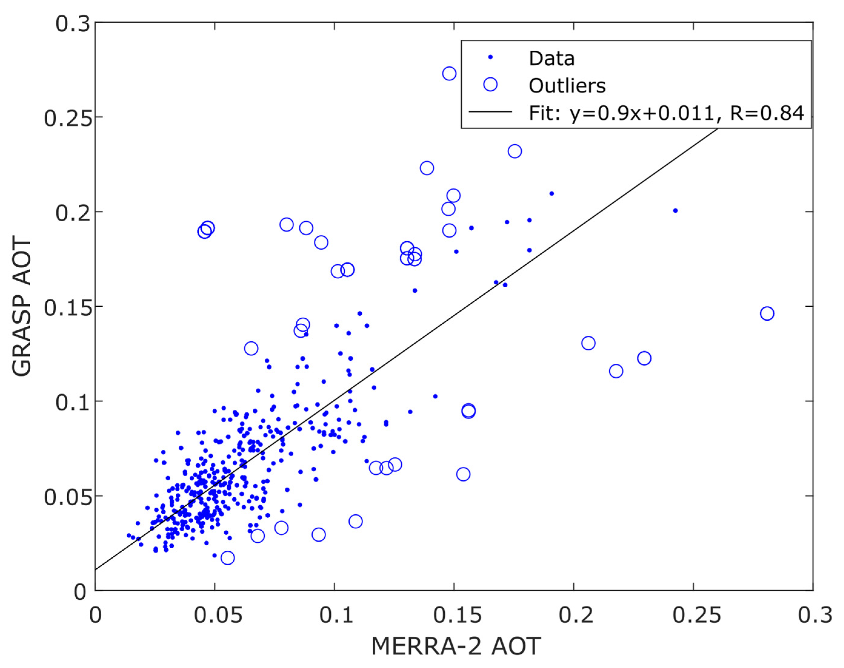
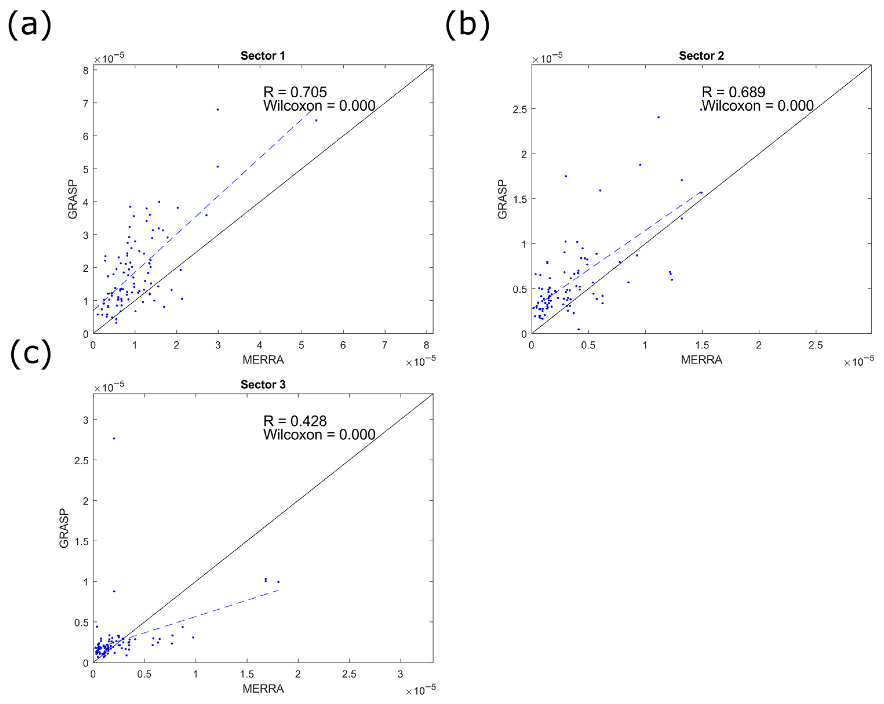
3.1. GRASP vs. MERRA2 Correlation

We conducted a comparison between the AOT values derived from the MERRA2 dataset and those obtained through GRASP (Figure 1). Data for the nearest grid point to the station location were chosen as representative of the studied location. We used GRASP and coincident MERRA-2 data only for cases when layers were manually recognized. Moreover, it is worth noting that the time between measured (GRASP) and modeled (MERRA-2) values may be up to 1.5 h, as MERRA-2 data are available in 3-h intervals.
The correlation coefficient (R) between the two datasets was calculated to be 0.84, indicating a strong linear relationship. However, a significant number of outliers, defined as exceeding 1.5 standard deviations, was observed for AOT, specifically when free tropospheric layers are present. These findings suggest that the aerosol modeling in the PBL is in good agreement between the two datasets. However, discrepancies arise when detached, high-altitude aerosol layers are present, indicated by a divergence between the modeled and retrieved values.
Detailed study and statistical analyses of both datasets were performed to better understand agreements and discrepancies for different altitudes and seasons.

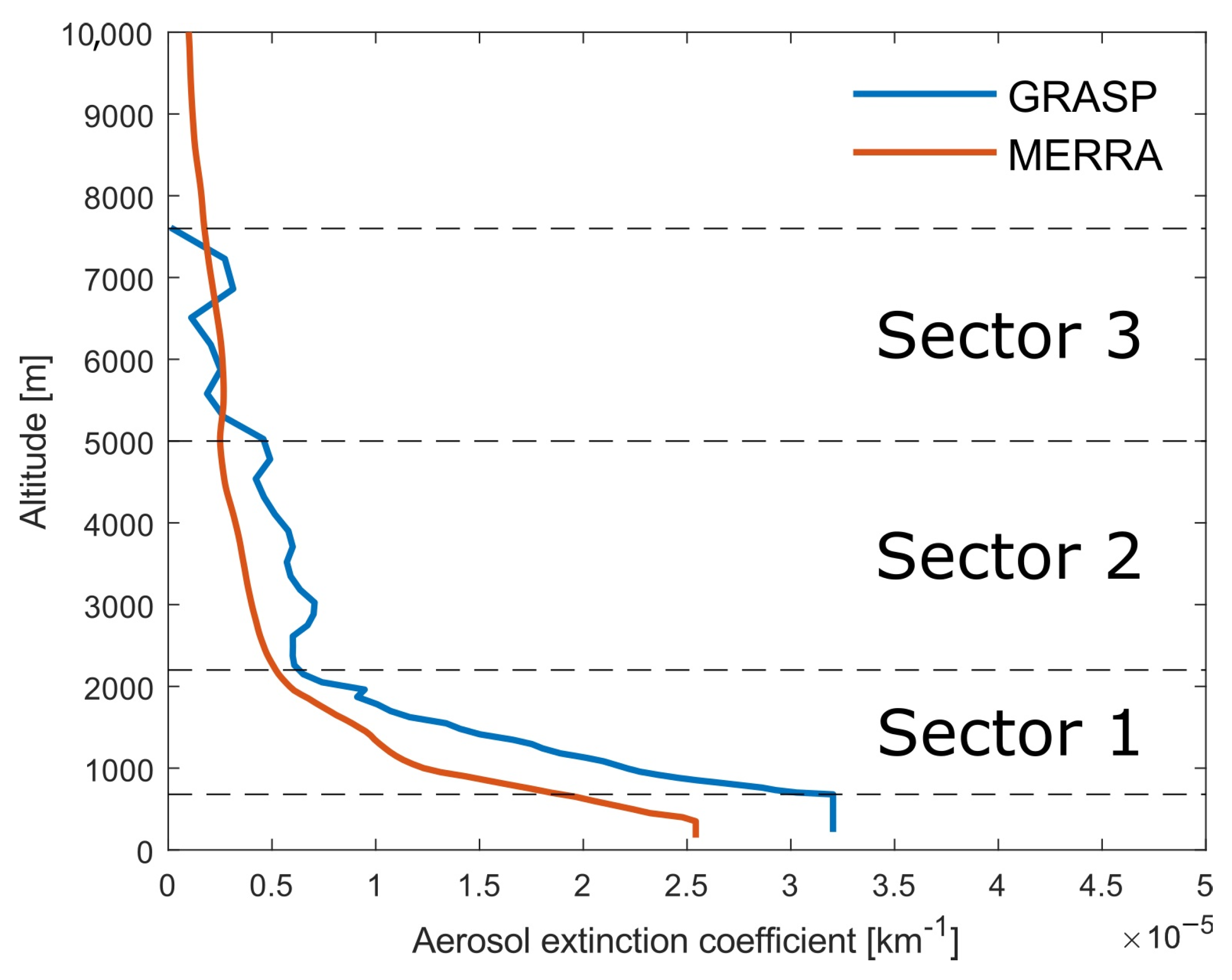
3.2. Vertical Extinction Profiles-GRASP vs. MERRA2

The high correlation coefficient between AOT values reproduced by GRASP and MERRA2 (R = 0.84), combined with a significant number of outliers in both distributions, necessitates further analysis of the vertical aerosol structure for a better understanding of the correspondence between the results yielded by the two approaches. To this end, we performed a statistical analysis of vertical profiles of aerosol extinction (α-profile) given by both GRASP and MERRA2 to quantify the differences at various altitudes. We analyzed the obtained profiles and identified altitude regions (hereafter called sectors) where we observed overall different behavior of the profile values and derivatives with height. Moreover, the vertical structure varies greatly with the seasons, predominantly within and immediately above the PBL. Thus, we divide our further analysis into warm (April–September) and cold (October–March) parts of the year.

3.2.1. Warm Season—Overview

During the warm season in Racibórz, we predominantly observed a convective diurnal evolution of the PBL. These conditions drive near-ground aerosols to higher altitudes during the first part of the day. The typical PBL top over Racibórz was observed at approximately 1500 m above the observatory, with most of the free-tropospheric aerosol layers located immediately above, within approximately 1 km. The remaining layers (with a few exceptions) were observed in the middle troposphere, roughly between 3 km and 5 km. To reflect the observed regimes in the vertical distribution of aerosols, we divided the observation domain into four sectors with boundaries at 680, 1700, 2800, 5000, and 7600 m. These values were selected manually at the “spikes” of the second vertical derivative of the averaged MERRA2 α-profile. The lowest and the highest values represent the lowermost full overlap altitude of the ceilometer and the highest altitude of GRASP retrieval, respectively. Figure 2 shows the averaged α-profiles and the selected sectors.

3.2.2. Cold Season—Overview

The cold part of the year is dominated by cases where the PBL was low and relatively stable. Thus, almost all of the layers were observed above the height of the diurnal PBL, mostly up to approximately 2200 m. Higher-altitude layers were retrieved by GRASP up to 5000 m, while MERRA2 shows a marked increase in aerosol load even higher, up to 8500 m. To reflect these observations, we chose to divide the observational domain into three sectors for the cold season, with thresholds at 680, 2200, 5000, and 7600 m. Similar to the warm season analysis, two external thresholds are enforced by minimal full overlap and by the top of the GRASP retrieval domain. The averaged α-profiles and the sector boundaries are shown in Figure 3.

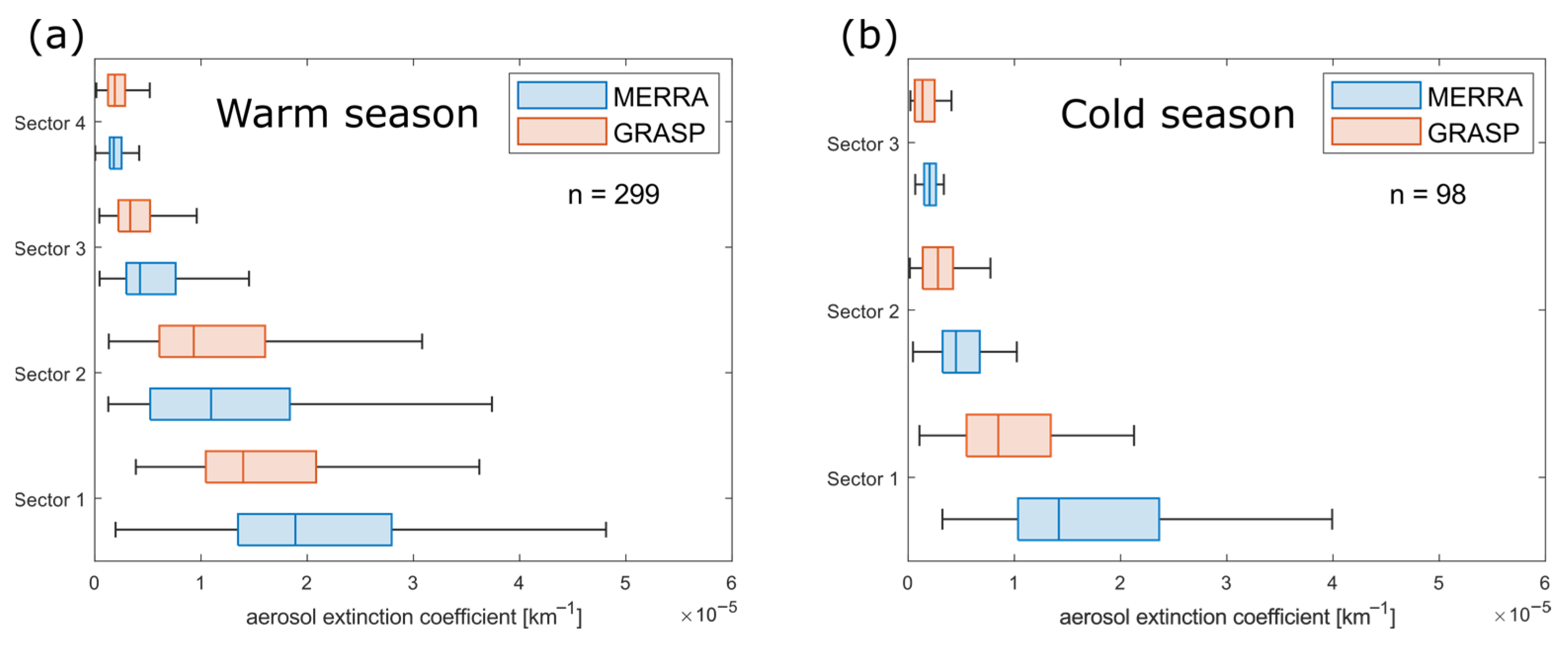
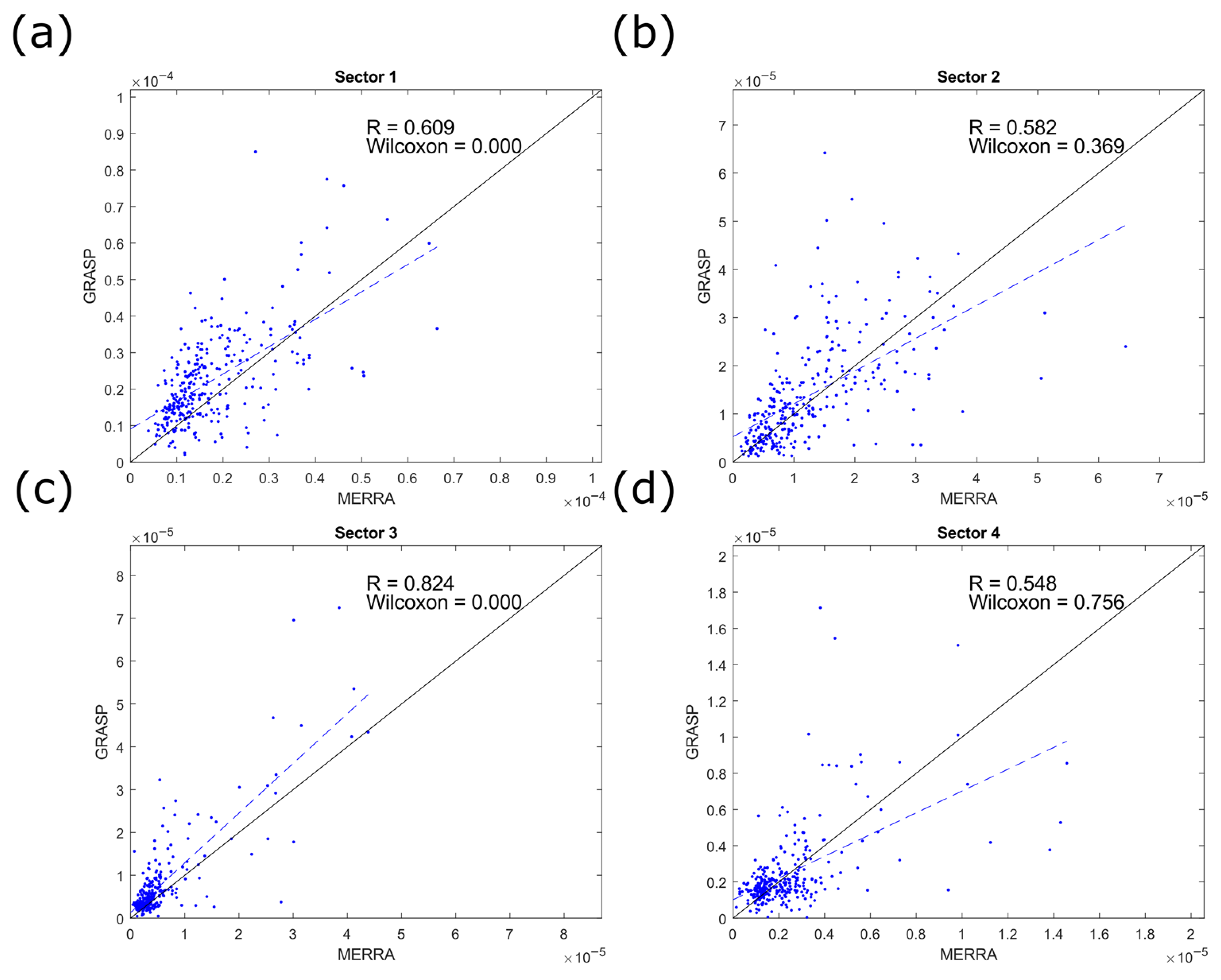
3.2.3. Statistical Analysis of the Aerosol Extinction within the Sectors

We start the statistical analysis by calculating average values within the sectors for individual profiles; thus, we represent each profile with four averages representative of the predefined sectors. The results are shown using box plots for MERRA2 and GRASP profiles in Figure 4.
To test the validity of the choice of the sectors, the pairs of the obtained populations are investigated using the Wilcoxon signed-rank test (Wilcoxon t-test). This test provides information on whether the two populations are statistically different from each other in the case of non-normal distributions. Populations of AOTs or extinctions are typically log-normal, as negative values cannot be observed. The performed analysis indicated a proper choice of sectors, as differences between sectors are statistically significant.
In addition, Wilcoxon analysis of MERRA2 vs. GRASP for each sector was performed for both the cold and warm parts of the year. Sample populations and the related median values differ significantly for most cases except Sectors 2 and 4 during the warm part of the year. This result is not surprising and confirms the difference between median values visible in Figure 4 and bias within sectors between the mean profiles visible in Figure 2 and Figure 3.
While a positive result of the Wilcoxon T-test indicates statistical differences between the populations, it does not provide information on the correlation between individual data points. In principle, a bias may be present between the data sets that will influence the medians and averages of the populations but not the correlations between the individual values. To analyze the co-behavior of GRASP and MERRA2 in the corresponding sectors, we prepared scatter plots for each pair of sectors, fitted straight lines to identify potential biases, and calculated correlation coefficients (R) for the population pairs. The results for warm and cold seasons are given in Figure 5 and Figure 6, respectively, along with the calculated values of the Pearson coefficient.
These results show an overall good (R > 0.5) correlation between GRASP and MERRA2 within sectors during the warm season. Sectors 1 and 3, which were identified to have statistically different median values, have the highest R values (~0.61 and ~0.82, respectively). This shows that, especially for sector 3 (middle troposphere), there are biases present between the populations. The remarkably high correlation coefficient in sector 3 indicates that while the models agree well on the altitude and time of occurrence of layers in this region, the retrieved values of extinction within the individual layers are consequently higher in GRASP profiles.
The correlations calculated for the cold season are high for sectors 1 and 2 (~0.71 and ~0.69, respectively) and moderate for sector 3 (~0.43). Strong biases are visible in sectors 1 and 2, as the GRASP retrieves significantly higher values in α-profiles compared to MERRA2. In the high troposphere (sector 3), the higher values are given by MERRA2. Episodes of high-altitude layers, associated with long-range transport, are occasionally modeled by MERRA2 but are not always retrieved by GRASP. The optical thickness of these layers is small, and thus it is probable that the ceilometer has an insufficient SNR to distinguish these layers from the noise.
The results of the proposed comparison between GRASP and MERRA2, in the scope of aerosol layer recognition in the free troposphere, show good agreement between the reanalysis and retrievals for most of the cases; however, bias was identified. The correlation coefficients between the averages calculated for sectors of individual α-profiles were moderate to high (>0.4) with the lowest values observed for the highest sectors, a representative of the high troposphere. This is most likely the direct result of the low SNR of the ceilometer in this region resulting in higher-than-desired variability of high-altitude GRASP retrievals. In most sectors, biases were observed towards GRASP profiles (i.e., GRASP retrieved denser aerosol layers than MERRA2). This may be a result of incorrect normalization of GRASP profiles to AOT from the sunphotometer, as the ceilometer profiles are available neither near the ground level nor in the high atmosphere (>~8 km). Note that our retrievals with GRASP assume negligible aerosol concentrations above the retrieval’s upper boundary of 7600 m, while MERRA2 routinely allocates a considerable amount of aerosol in higher altitudes.

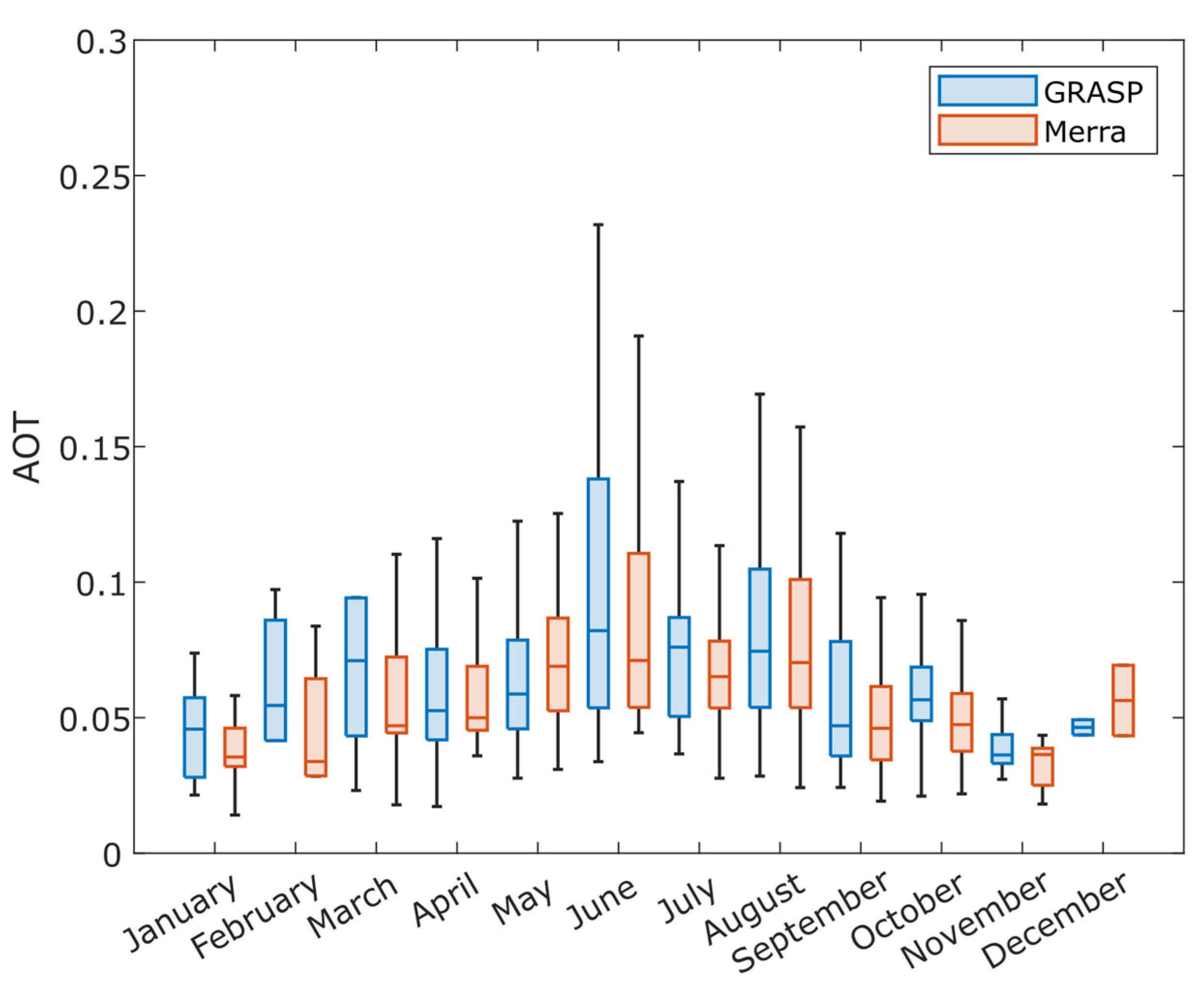
3.3. Seasonal Variability of Aerosol Optical Thickness

We examined the optical depth of atmospheric aerosols, including both the cumulative columnar values and the contributions of individual layers. We compared the AOT obtained from photometric measurements with the values provided by MERRA2. The results are shown in Figure 7. It should be noted that the total AOT only encompasses cases where layers were detected.
Our analysis reveals two prominent peaks in AOT, occurring in June and August. However, no significant peak is observed during the spring season, which is typically associated with biomass-burning episodes or accumulation of aerosols in the boundary layer during the slow movement of an air mass. Mentioned yearly patterns with two seasonal peaks were found for central Poland [40,73] and the Tatra Mountains [74]. We identify two distinct regimes based on the time of the year: a warm period characterized by higher AOT values, and a cold period with lower AOT values. We consistently observe higher AOT values from our retrievals compared to the values obtained from MERRA2. This discrepancy suggests that some aerosol layers might be missing in the reanalysis data or that the amount of aerosol in the free troposphere is underestimated in the transport model.

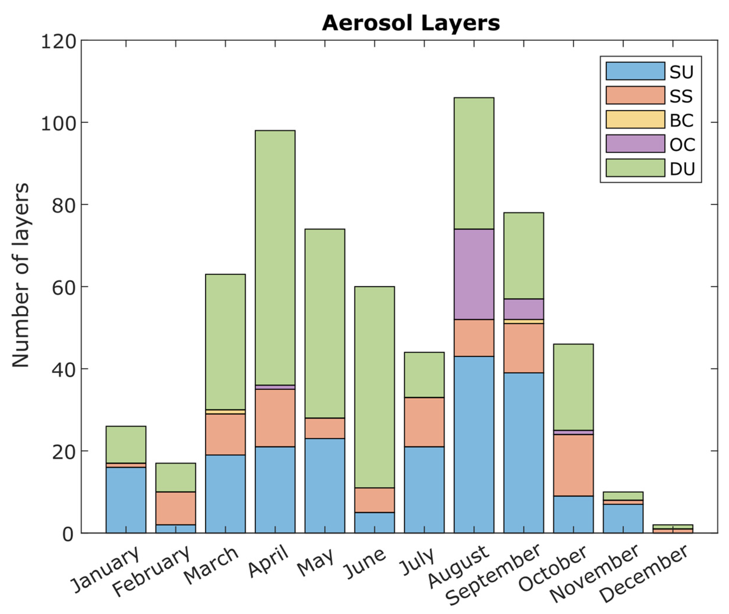
3.4. Aerosol Typing within Layers

Our analysis, depicted in Figure 8, reveals two prominent peaks in the number of identified layers, occurring in April and August. However, it is important to note that the high number of layers observed in April does not correspond to high AOT values, as depicted in Figure 7. This observation suggests that most layers identified in April are optically thin.
Further investigation indicated that over 50% of the layers identified in April were attributed to dust particles. This finding suggested that the high number of layers during this period was driven primarily by the advection of dust particles from the Sahara at high altitudes.
A high contribution of DU in the free troposphere is observed throughout the year, likely associated with the long-range advection of the Saharan dust. This is supported by many previous studies, e.g., [75,76]. Our analysis shows a large number of DU layers in the spring season, which could be linked to local agricultural activities. Specifically, freshly plowed soil, which is devoid of vegetation, is prone to wind-driven erosion, leading to the generation of dust particles.
Additionally, we have observed the presence of OC from biomass-burning episodes during the late summer season. Our findings suggest that the high temperatures and low humidity during this period increase the probability of wildfires, resulting in the release of OC into the atmosphere. Vertical distribution of layers indicates high-altitude trans-Atlantic OC aerosol advection from North America. Such layers have been observed over Europe in several studies, e.g., [77,78].
Moreover, sea salt particles exhibit a significant contribution throughout the year, which agrees with results provided by various chemical models, e.g., [79,80]. Our findings align with the advection patterns originating from the Baltic and the North Sea (see Section 3.6.3).

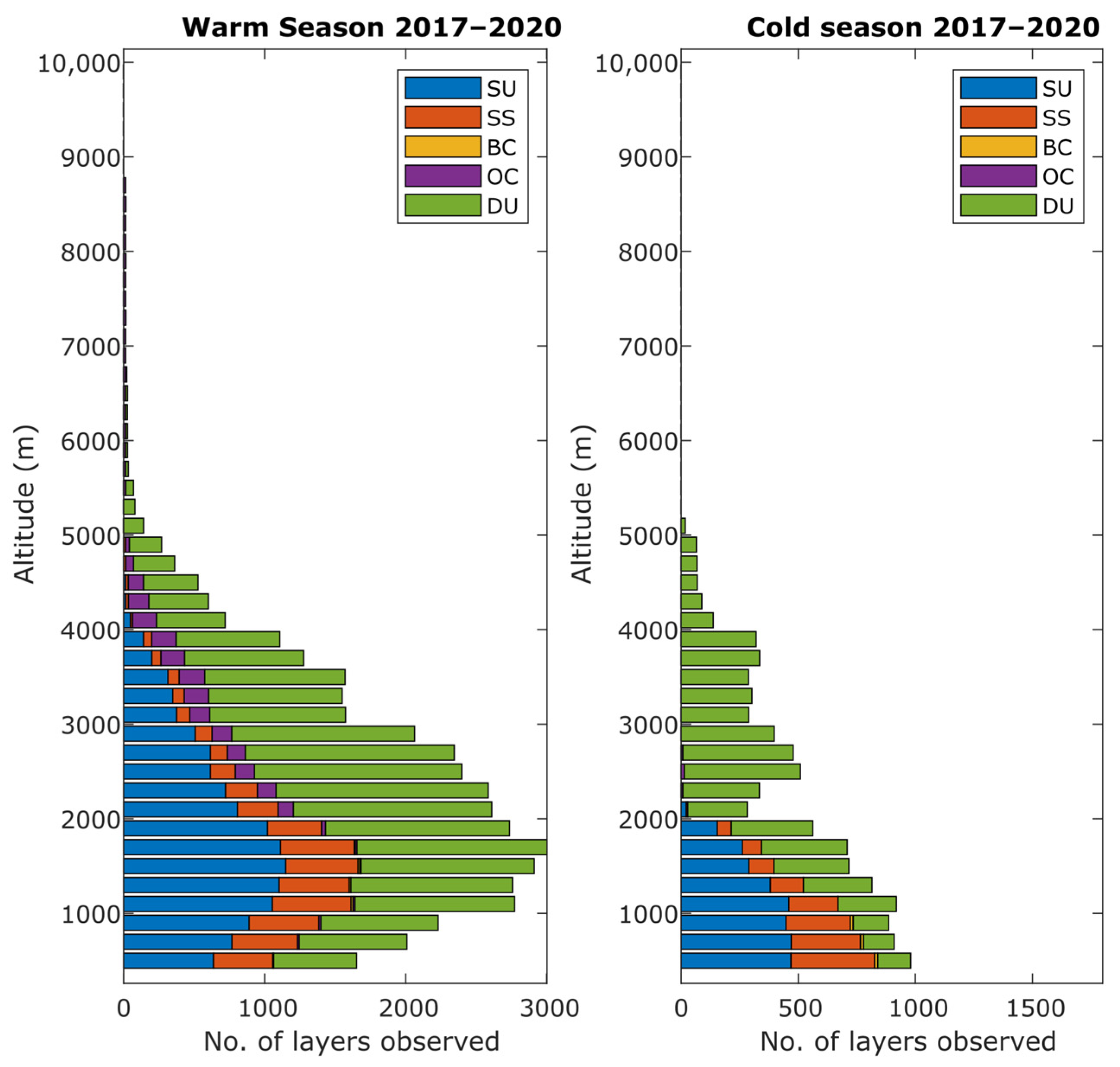
3.5. Vertical Distribution of Aerosol Species

The vertical distribution of aerosol layers within the entire dataset is presented in Figure 9, with each layer identified based on the dominant aerosol species provided by MERRA2. Percentage composition of the aerosol type for each consecutive one kilometer range is given in Table 1.
The maximum number of identified layers is observed at approximately 2000 m, while very few cases are observed above 6000 m. These high-altitude cases are predominantly characterized by OC aerosols, indicating trans-Atlantic transport. Sea salt aerosols are primarily observed closer to the ground, with the highest concentration occurring at 1200 m. This observation is in agreement with the absence of strong convection over the seas. However, the unexpectedly strong contribution of sea salt aerosols may be an artifact of the model and requires further investigation. One possible explanation is that these were continental aged aerosols, with low AODs and moderate AE values, which were misidentified as sea salt aerosol.
Mineral aerosols, specifically dust particles, contribute significantly to pollution at lower altitudes and become the dominant contaminant above approximately 2 km. This finding suggests a mixture of both local sources (such as agricultural activities and wind-driven soil erosion) and remote sources (such as Saharan dust). Sulfate-rich layers, characteristic of continental anthropogenic pollution, are mainly present in the low troposphere, up to 4 km. This indicates local emissions and short-distance advection. In contrast, organic carbon aerosols are observed at higher altitudes, predominantly above 2 km. This type of aerosol is often observed during the eastward advection of air masses traveling over both natural and human-induced fires in eastern Europe [39]. These biomass-burning aerosols travel at higher altitudes, above the PBL, and can become the dominant species in the free tropospheric layers over Poland.
It is important to note that the analysis specifically focuses on free tropospheric or residual layers and excludes aerosols within the convectively active boundary layer. This has two identifiable consequences. Firstly, the number of free tropospheric layers decreases near the ground, as the height of the PBL oscillates between approximately 100 m during winter and 1.5–2 km during the summer season. This effect is an artifact of the chosen analysis scheme and does not carry scientific significance. Secondly, the contribution from BC aerosols, associated with low emissions and coal burning, is very low. This is attributed to the fact that BC emissions predominantly occur during the colder half of the year when the PBL is typically low and convectively stable, e.g., [81,82], resulting in minimal aerosol entrainment into the free troposphere.

3.6. Backward Trajectory Statistics—Geographical Validation of Aerosol Layer Typing

To test the performance of the proposed method for aerosol layer identification and type recognition, we employed a previously developed scheme for air mass backward trajectory statistics. We selected altitude regions shown in the previous Section 3.4 to be populated by layers of a certain aerosol type. Next, we calculated backward trajectories with endpoints spatially and temporally collocated with individual identified layers dominated by said aerosol type. Finally, we used the statistical method described in Section 2.2.3 to reveal potential source regions of the selected aerosol layers.

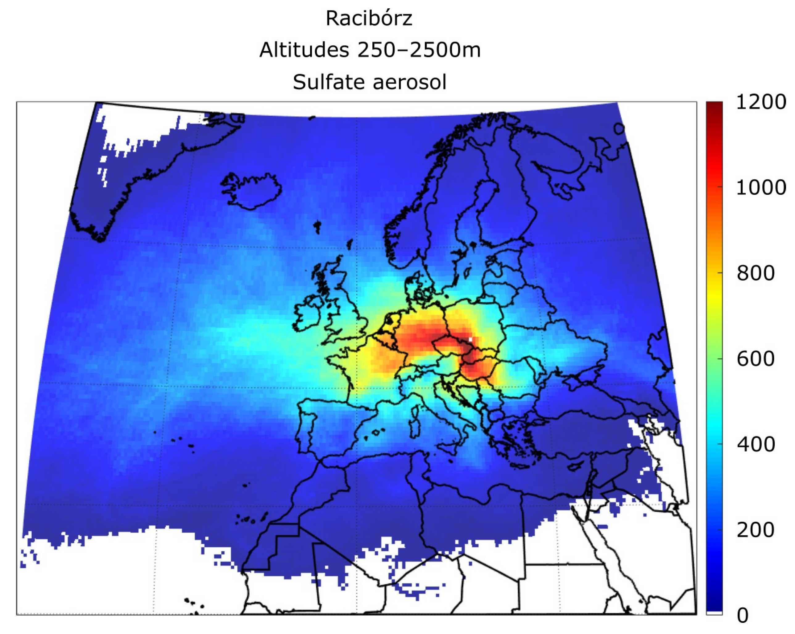
3.6.1. Sulphate Aerosols

The primary sources of sulfate pollutants in the area are likely to be anthropogenic in nature, including activities such as industrial operations, household heating, transportation, and biomass burning. The observed trajectory pattern (Figure 10) supports this notion as the identified potential sources are predominantly located over the densely populated landmass of the European continent. Notably, the trajectory paths demonstrate the presence of the Moravian Gate, a prominent geographic feature in the region.

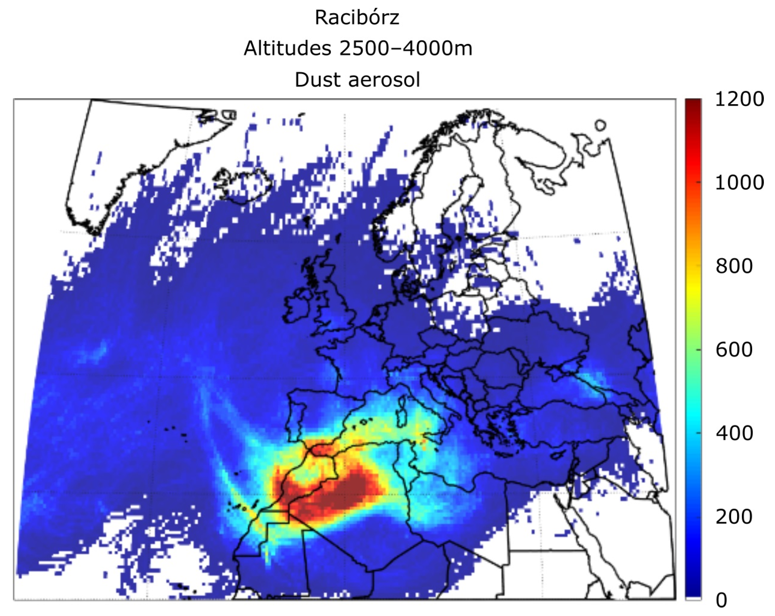
3.6.2. Dust Aerosols

The strongest source of airborne dust particles in the vicinity of Europe is the Sahara, due to both the abundance of very fine sand material and the very strong convection that develops over the desert during daytime with the PBL top often reaching 5 km above the surface. Potential sources of dust aerosols were identified south of the Sierra Nevada and Atlas Mountain ranges (Figure 11). These aerosols were likely uplifted by air mass on the slopes of these mountain ranges and subsequently transported over the Atlantic and Mediterranean regions.

3.6.3. Sea Salt Aerosols

Sea salt aerosols are produced predominantly over large bodies of water during high-wind conditions; thus, we expect the Baltic, North Sea, and the greater Atlantic to be the primary sources for Racibórz. While the two latter are clearly visible in the result of the analysis (Figure 12), the lack of sources over the Baltic is puzzling. One possible explanation is that the overall domination of western advection over central Europe makes it unlikely for aim masses to travel approximately 1000 km south from above the Baltic.
An interesting artifact observed in the trajectory pattern is the presence of a cone-shaped feature near Racibórz, which has been demonstrated in previous studies to emerge between far-removed sources (in this case over the North Atlantic) and the receptor when no nearby sources are present.

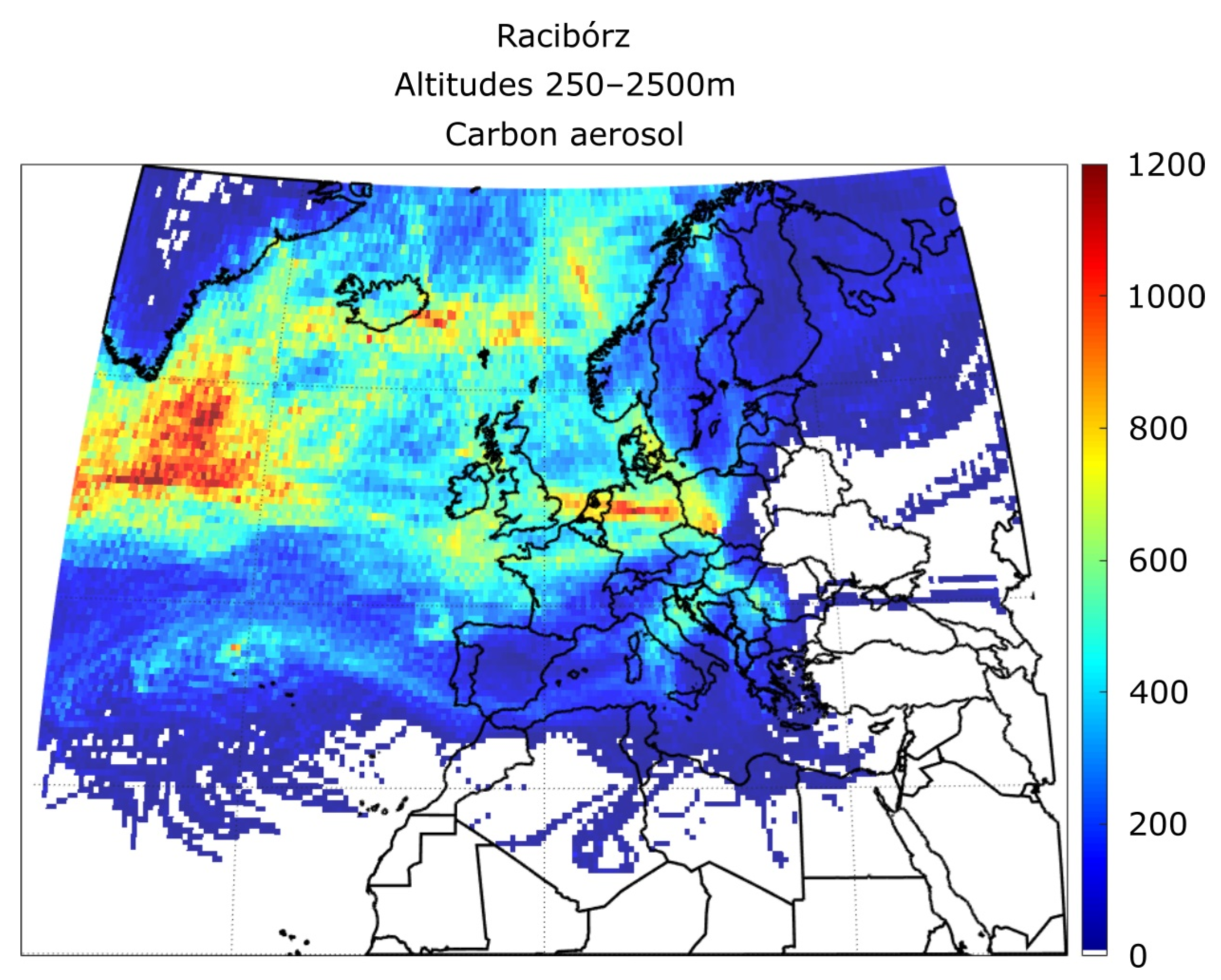
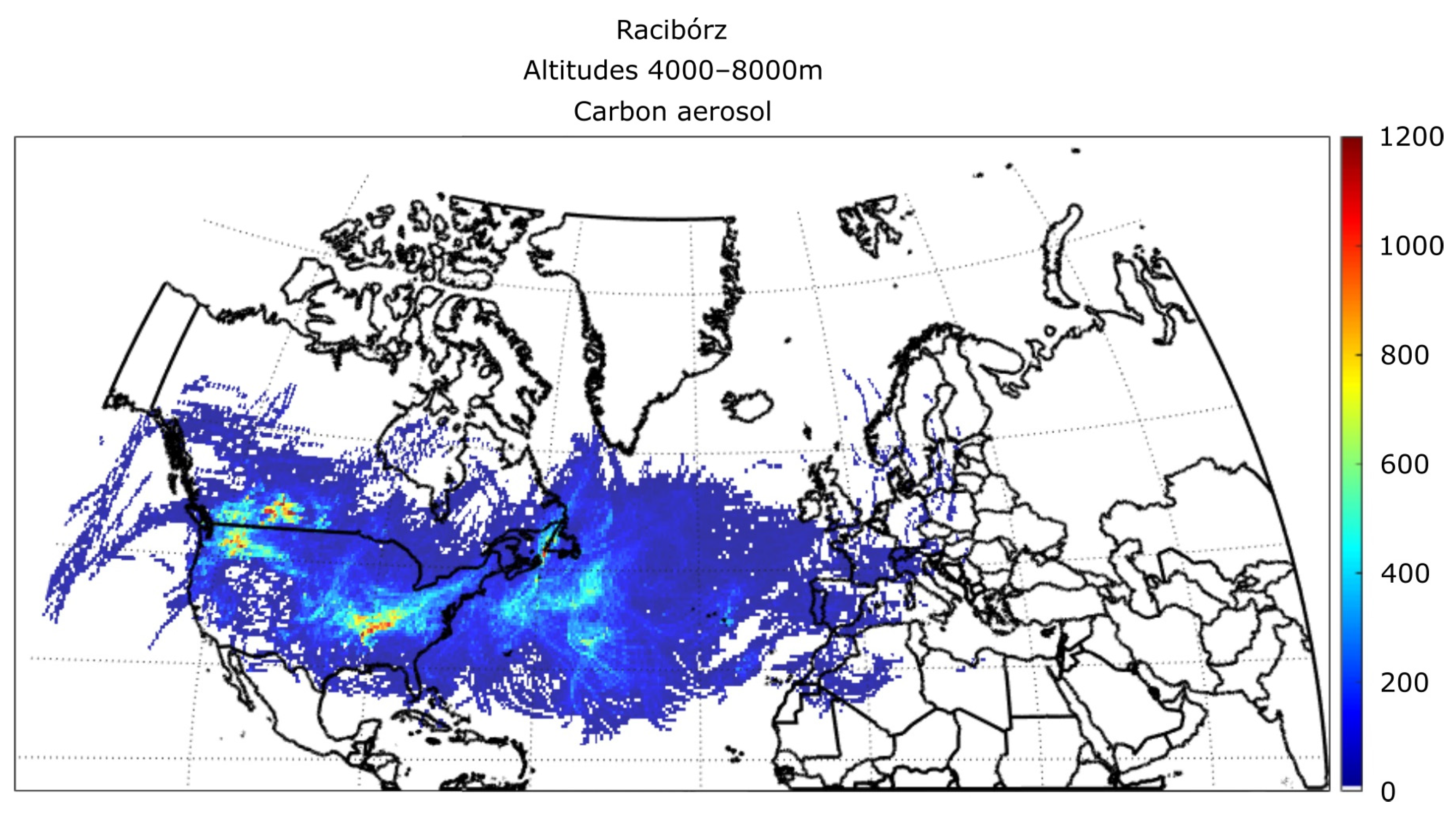
3.6.4. Carbonous Aerosols

A strong hot spot for carbon aerosols is clearly discernible in central-western Europe, indicating the influence of heavy industrial activities in the region (Figure 13). Additionally, sources of carbon aerosols were also observed in the eastern part of the region, likely attributable to biomass-burning activities.
Interestingly, an unidentified source of carbon aerosols was observed over the North Atlantic, west of Ireland, necessitating further investigation to ascertain its origin and transport pathways. The presence of carbon aerosols in this area implies the potential contribution of long-range transport from other regions, likely at higher altitudes. To test this hypothesis, we expanded our analysis with faint, high-altitude layers identified mostly during the cold season.
The trans-Atlantic transport of OC aerosols, depicted in Figure 14, emerges as a significant source of carbon aerosols within the region. The study identifies specific sources of carbon aerosols over the Rocky Mountains at the USA-Canada border and the Appalachians in the eastern USA. These sources can be attributed to large forest fires occurring on mountain slopes, where orography-supported convection lifts the aerosols up to 4–5 km above sea level. These regions act as primary contributors of carbon aerosols in the area.

4. Discussion

The performance of the GRASP and MERRA2 models was compared in terms of reproducing aerosol layers. Overall, a satisfactory agreement was observed between the two models. Although a high correlation was evident, discrepancies in median values across various sectors indicated the presence of biases. Specifically, GRASP exhibited denser aerosol layers in the mid-troposphere, while MERRA2 allocated a significant amount of aerosol around the tropopause and even in the low stratosphere. One limitation of GRASP was its inability to provide information near the ground, primarily due to issues related to normalizing columnar AOT. Addressing the observed biases can potentially allow for improved agreement between GRASP and MERRA2. This can be accomplished by utilizing stronger LIDAR instruments for high-altitude retrievals and closing profiles at ground level using multi-angle nephelometer retrievals specifically tailored for the GRASP model.
When analyzing the MERRA dataset, the profile shows the maximum amount of dust. This could be due to the type of dataset used, as MERRA models dust into five bins, and for this analysis, the sum total of all the bins was used. Furthermore, such variation of aerosol species at different altitudes highlights the importance of understanding the sources and transport pathways of aerosols in the region to better understand the distribution and impacts of atmospheric pollutants.
We observed limited instances of BC or OC dominant layers. This is likely due to the underestimation of BC and OC by the MERRA-2 model when considering other aerosol species. Ref. [83] made a similar observation using satellite remote-sensing data from PARASOL/GRASP. They retrieved global emissions of BC, OC, and dust aerosols and found significant underestimations compared to model inventories. BC emissions were 166.7% higher, while OC emissions were 184.0% higher than the inventories.
Moreover, our findings suggest that the limited presence of sea salt aerosols at higher altitudes indicates the importance of understanding local and regional factors that influence the distribution of atmospheric pollutants. Further research is needed to better understand the sources and transport pathways of these aerosols in the region.
The atmospheric composition over the Racibórz station is influenced by a complex interplay of various factors such as advection, orography, and altitude-dependent potential sources for individual dominant species. This complexity is reflected in the mixture of both local and long-range sources of pollutants, highlighting the need to consider atmospheric dynamics and transport when studying the distribution of pollutants in the region.

5. Conclusions

In this study, we used a combination of GRASP and MERRA2 models to identify aerosol layers in the atmosphere, while MERRA2 data on aerosol mixture allowed for identification of the dominant aerosol species in each detected layer. Moreover, statistical analysis of advection patterns of selected aerosol species was performed to validate our aerosol type recognition. We deem the result to be satisfactory, as all the primary species’ sources were located in the regions that are likely sources of the investigated species. Our approach enables the identification of seasonal pollution transport patterns and provides good identification of dust advection episodes and corresponding source appointments. Additionally, our method allows for confirmation of biomass-burning advection through the free troposphere, including mid- to long-range transport, even trans-Atlantic.
Our analysis also reveals that the variation in trajectory patterns at different altitudes underscores the importance of understanding atmospheric dynamics and transport in the region. Dust aerosols were found to have significant impacts on air quality, human health, and climate, highlighting the need for continued monitoring and research to better understand their sources and transport pathways. Overall, our study highlights the importance of considering the complex interplay of various factors that influence atmospheric composition and transport in the region to improve our understanding of air quality and its impacts on human health and climate.

Author Contributions

Conceptualization, A.F., A.S. and A.P.; methodology, A.F., A.S. and A.P.; software, A.F., A.S. and A.P.; validation, A.F. and A.S.; formal analysis, A.F., A.S. and A.P.; investigation, A.F., A.S. and A.P.; resources, A.F.; data curation, A.F.; writing—original draft preparation, A.F., A.S. and A.P.; visualization, A.F., A.S. and A.P.; supervision, A.S. and A.P.; project administration, A.P.; funding acquisition, A.P. All authors have read and agreed to the published version of the manuscript.

Funding

This research was funded by National Science Centre, Poland, grant number 2017/25/B/ST10/01650.

Institutional Review Board Statement

Not applicable.

Informed Consent Statement

Not applicable.

Data Availability Statement

MERRA-2 data are available publicly at https://disc.gsfc.nasa.gov/datasets?project=MERRA-2. The lidar data presented in this study are available on request from the corresponding author.

Conflicts of Interest

The authors declare no conflict of interest.

References

  1. Myhre, G.; Myhre, C.E.L.; Samset, B.H.; Storelvmo, T. Aerosols and Their Relation to Global Climate and Climate Sensitivity. Nat. Educ. Knowl. 2013, 4, 7. [Google Scholar]
  2. Zhang, B.; Zhang, B. The Effect of Aerosols to Climate Change and Society. J. Geosci. Environ. Prot. 2020, 8, 55–78. [Google Scholar] [CrossRef]
  3. Bellouin, N.; Quaas, J.; Gryspeerdt, E.; Kinne, S.; Stier, P.; Watson-Parris, D.; Boucher, O.; Carslaw, K.S.; Christensen, M.; Daniau, A.L.; et al. Bounding Global Aerosol Radiative Forcing of Climate Change. Rev. Geophys. 2020, 58, e2019RG000660. [Google Scholar] [CrossRef] [PubMed]
  4. Zhang, R.-J.; Ho, K.-F.; Shen, Z.-X. The Role of Aerosol in Climate Change, the Environment, and Human Health. New Pub. KeAi 2015, 5, 156–161. [Google Scholar] [CrossRef]
  5. Sosnowski, T.R. Aerosols and human health—A multiscale problem. Chem. Eng. Sci. 2023, 268, 118407. [Google Scholar] [CrossRef]
  6. Air Quality in Europe—2020 Report; European Environment Agency: Copenhagen, Denmark, 2020.
  7. Pietruczuk, A.; Fernandes, A.; Szkop, A.; Krzyścin, J. Impact of Vertical Profiles of Aerosols on the Photolysis Rates in the Lower Troposphere from the Synergy of Photometer and Ceilometer Measurements in Raciborz, Poland, for the Period 2015–2020. Remote Sens. 2022, 14, 1057. [Google Scholar] [CrossRef]
  8. Fernandes, A.; Pietruczuk, A.; Szkop, A.; Krzyścin, J. Aerosol Layering in the Free Troposphere over the Industrial City of Raciborz in Southwest Poland and Its Influence on Surface UV Radiation. Atmosphere 2021, 12, 812. [Google Scholar] [CrossRef]
  9. Heicklen, J. Atmospheric lifetimes of pollutants. Atmos. Environ. 1982, 16, 821–823. [Google Scholar] [CrossRef]
  10. Akimoto, H. Global Air Quality and Pollution. Science 2003, 302, 1716–1719. [Google Scholar] [CrossRef]
  11. Andreae, M.O. Aerosols before pollution. Science 2007, 315, 50–51. [Google Scholar] [CrossRef]
  12. Baker, L.H.; Collins, W.J.; Olivié, D.J.L.; Cherian, R.; Hodnebrog; Myhre, G.; Quaas, J. Climate responses to anthropogenic emissions of short-lived climate pollutants. Atmos. Chem. Phys. 2015, 15, 8201–8216. [Google Scholar] [CrossRef]
  13. Szkop, A.; Pietruczuk, A. Analysis of aerosol transport over southern Poland in August 2015 based on a synergy of remote sensing and backward trajectory techniques. J. Appl. Remote Sens. 2017, 11, 016039. [Google Scholar] [CrossRef]
  14. Daskalakis, N.; Myriokefalitakis, S.; Kanakidou, M. Sensitivity of tropospheric loads and lifetimes of short lived pollutants to fire emissions. Atmos. Chem. Phys. 2015, 15, 3543–3563. [Google Scholar] [CrossRef]
  15. Cárdenas Rodríguez, M.; Dupont-Courtade, L.; Oueslati, W. Air pollution and urban structure linkages: Evidence from European cities. Renew. Sustain. Energy Rev. 2016, 53, 1–9. [Google Scholar] [CrossRef]
  16. Szkop, A.; Pietruczuk, A.; Posyniak, M. Classification of aerosol over central Europe by cluster analysis of aerosol columnar optical properties and backward trajectory statistics. Acta Geophys. 2016, 64, 2650–2676. [Google Scholar] [CrossRef]
  17. Sinha, P.R.; Manchanda, R.K.; Kaskaoutis, D.G.; Kumar, Y.B.; Sreenivasan, S. Seasonal variation of surface and vertical profile of aerosol properties over a tropical urban station Hyderabad, India. J. Geophys. Res. Atmos. 2013, 118, 749–768. [Google Scholar] [CrossRef]
  18. Benavent-Oltra, J.A.; Román, R.; Andrés Casquero-Vera, J.; Pérez-Ramírez, D.; Lyamani, H.; Ortiz-Amezcua, P.; Bedoya-Velásquez, A.E.; De Arruda Moreira, G.; Barreto, Á.; Lopatin, A.; et al. Different strategies to retrieve aerosol properties at night-time with the GRASP algorithm. Atmos. Chem. Phys. 2019, 19, 14149–14171. [Google Scholar] [CrossRef]
  19. Kabashnikov, V.; Milinevsky, G.; Chaikovsky, A.; Miatselskaya, N.; Danylevsky, V.; Aculinin, A.; Kalinskaya, D.; Korchemkina, E.; Bovchaliuk, A.; Pietruczuk, A.; et al. Localization of aerosol sources in East-European region by back-trajectory statistics. Int. J. Remote Sens. 2014, 35, 6993–7006. [Google Scholar] [CrossRef]
  20. Madonna, F.; Amato, F.; Vande Hey, J.; Pappalardo, G. Ceilometer aerosol profiling versus Raman lidar in the frame of the INTERACT campaign of ACTRIS. Atmos. Meas. Tech. 2015, 8, 2207–2223. [Google Scholar] [CrossRef]
  21. Comerón, A.; Muñoz-Porcar, C.; Rocadenbosch, F.; Rodríguez-Gómez, A.; Sicard, M. Current Research in Lidar Technology Used for the Remote Sensing of Atmospheric Aerosols. Sensors 2017, 17, 1450. [Google Scholar] [CrossRef]
  22. Dang, R.; Yang, Y.; Hu, X.M.; Wang, Z.; Zhang, S. A Review of Techniques for Diagnosing the Atmospheric Boundary Layer Height (ABLH) Using Aerosol Lidar Data. Remote Sens. 2019, 11, 1590. [Google Scholar] [CrossRef]
  23. Zhang, Q.; Jimenez, J.L.; Canagaratna, M.R.; Ulbrich, I.M.; Ng, N.L.; Worsnop, D.R.; Sun, Y. Understanding atmospheric organic aerosols via factor analysis of aerosol mass spectrometry: A review. Anal. Bioanal. Chem. 2011, 401, 3045–3067. [Google Scholar] [CrossRef]
  24. Boucher, O. Atmospheric Aerosols, 1st ed.; Springer: Dordrecht, The Netherlands, 2015; ISBN 978-94-017-9648-4. [Google Scholar]
  25. Holben, B.N.; Eck, T.F.; Slutsker, I.; Smirnov, A.; Sinyuk, A.; Schafer, J.; Giles, D.; Dubovik, O. Aeronet’s Version 2.0 quality assurance criteria. In Remote Sensing of the Atmosphere and Clouds; Tsay, S.-C., Nakajima, T., Singh, R.P., Sridharan, R., Eds.; SPIE: Bellingham, WA, USA, 2006; Volume 6408. [Google Scholar]
  26. Sinyuk, A.; Holben, B.N.; Eck, T.F.; Giles, D.M.; Giles, D.; Slutsker, I.; Korkin, S.; Schafer, J.S.; Smirnov, A.; Sorokin, M.; et al. The AERONET Version 3 aerosol retrieval algorithm, associated uncertainties and comparisons to Version 2. Atmos. Meas. Tech. 2020, 13, 3375–3411. [Google Scholar] [CrossRef]
  27. Torres, B.; Fuertes, D. Characterization of aerosol size properties from measurements of spectral optical depth: A global validation of the GRASP-AOD code using long-term AERONET data. Atmos. Meas. Tech. 2021, 14, 4471–4506. [Google Scholar] [CrossRef]
  28. Lee, J.; Kim, J.; Song, C.H.; Kim, S.B.; Chun, Y.; Sohn, B.J.; Holben, B.N. Characteristics of aerosol types from AERONET sunphotometer measurements. Atmos. Environ. 2010, 44, 3110–3117. [Google Scholar] [CrossRef]
  29. Dionisi, D.; Barnaba, F.; Diémoz, H.; Di Liberto, L.; Gobbi, G.P. A multiwavelength numerical model in support of quantitative retrievals of aerosol properties from automated lidar ceilometers and test applications for AOT and PM10 estimation. Atmos. Meas. Tech. 2018, 11, 6013–6042. [Google Scholar] [CrossRef]
  30. Perrone, M.R.; De Tomasi, F.; Gobbi, G.P. Vertically resolved aerosol properties by multi-wavelength lidar measurements. Atmos. Chem. Phys. 2014, 14, 1185–1204. [Google Scholar] [CrossRef]
  31. Balis, D.S.; Amiridis, V.; Zerefos, C.; Gerasopoulos, E.; Andreae, M.; Zanis, P.; Kazantzidis, A.; Kazadzis, S.; Papayannis, A. Raman lidar and sunphotometric measurements of aerosol optical properties over Thessaloniki, Greece during a biomass burning episode. Atmos. Environ. 2003, 37, 4529–4538. [Google Scholar] [CrossRef]
  32. Lopatin, A.; Dubovik, O.; Chaikovsky, A.; Goloub, P.; Lapyonok, T.; Tanré, D.; Litvinov, P. Enhancement of aerosol characterization using synergy of lidar and sun-photometer coincident observations: The GARRLiC algorithm. Atmos. Meas. Tech. 2013, 6, 2065–2088. [Google Scholar] [CrossRef]
  33. Konsta, D.; Tsekeri, A.; Solomos, S.; Siomos, N.; Gialitaki, A.; Tetoni, E.; Lopatin, A.; Goloub, P.; Dubovik, O.; Amiridis, V.; et al. The Potential of GRASP/GARRLiC Retrievals for Dust Aerosol Model Evaluation: Case Study during the PreTECT Campaign. Remote Sens. 2021, 13, 873. [Google Scholar] [CrossRef]
  34. Lopatin, A.; Dubovik, O.; Fuertes, D.; Stenchikov, G.; Lapyonok, T.; Veselovskii, I.; Wienhold, F.G.; Shevchenko, I.; Hu, Q.; Parajuli, S. Synergy processing of diverse ground-based remote sensing and in situ data using the GRASP algorithm: Applications to radiometer, lidar and radiosonde observations. Atmos. Meas. Tech. 2021, 14, 2575–2614. [Google Scholar] [CrossRef]
  35. Dubovik, O.; Lapyonok, T.; Litvinov, P.; Herman, M.; Fuertes, D.; Ducos, F.; Torres, B.; Derimian, Y.; Huang, X.; Lopatin, A.; et al. GRASP: A versatile algorithm for characterizing the atmosphere. SPIE Newsroom 2014, 25, 4. [Google Scholar] [CrossRef]
  36. Molero, F.; Pujadas, M.; Artíñano, B. Study of the Effect of Aerosol Vertical Profile on Microphysical Properties Using GRASP Code with Sun/Sky Photometer and Multiwavelength Lidar Measurements. Remote Sens. 2020, 12, 4072. [Google Scholar] [CrossRef]
  37. López-Cayuela, M.Á.; Herrera, M.E.; Córdoba-Jabonero, C.; Pérez-Ramírez, D.; Carvajal-Pérez, C.V.; Dubovik, O.; Guerrero-Rascado, J.L. Retrieval of Aged Biomass-Burning Aerosol Properties by Using GRASP Code in Synergy with Polarized Micro-Pulse Lidar and Sun/Sky Photometer. Remote Sens. 2022, 14, 3619. [Google Scholar] [CrossRef]
  38. Román, R.; Benavent-Oltra, J.A.; Casquero-Vera, J.A.; Lopatin, A.; Cazorla, A.; Lyamani, H.; Denjean, C.; Fuertes, D.; Pérez-Ramírez, D.; Torres, B.; et al. Retrieval of aerosol profiles combining sunphotometer and ceilometer measurements in GRASP code. Atmos. Res. 2018, 204, 161–177. [Google Scholar] [CrossRef]
  39. Szkop, A.; Pietruczuk, A. Synergy of satellite-based aerosol optical thickness analysis and trajectory statistics for determination of aerosol source regions. Int. J. Remote Sens. 2019, 40, 8450–8464. [Google Scholar] [CrossRef]
  40. JarosŁawski, J.; Pietruczuk, A. On the origin of seasonal variation of aerosol optical thickness in UV range over Belsk, Poland. Acta Geophys. 2010, 58, 1134–1146. [Google Scholar] [CrossRef]
  41. Markowicz, K.M.; Stachlewska, I.S.; Zawadzka-Manko, O.; Wang, D.; Kumala, W.; Chilinski, M.T.; Makuch, P.; Markuszewski, P.; Rozwadowska, A.K.; Petelski, T.; et al. A Decade of Poland-AOD Aerosol Research Network Observations. Atmosphere 2021, 12, 1583. [Google Scholar] [CrossRef]
  42. Holben, B.N.; Tanré, D.; Smirnov, A.; Eck, T.F.; Slutsker, I.; Dubovik, O.; Lavenu, F.; Abuhassen, N.; Châtenet, B. Optical Properties of Aerosols from Long Term Ground-Based AERONET Measurements. 1999. Available online: https://ntrs.nasa.gov/citations/19990046554 (accessed on 1 August 2023).
  43. Holben, B.N.; Eck, T.F.; Slutsker, I.; Tanré, D.; Buis, J.P.; Setzer, A.; Vermote, E.; Reagan, J.A.; Kaufman, Y.J.; Nakajima, T.; et al. AERONET—A federated instrument network and data archive for aerosol characterization. Remote Sens. Environ. 1998, 66, 1–16. [Google Scholar] [CrossRef]
  44. Eck, T.F.; Holben, B.N.; Slutsker, I.; Setzer, A. Measurements of irradiance attenuation and estimation of aerosol single scattering albedo for biomass burning aerosols in Amazonia. J. Geophys. Res. Atmos. 1998, 103, 31865–31878. [Google Scholar] [CrossRef]
  45. Smirnov, A.; Holben, B.N.; Eck, T.F.; Dubovik, O.; Slutsker, I. Cloud-screening and quality control algorithms for the AERONET database. Remote Sens. Environ. 2000, 73, 337–349. [Google Scholar] [CrossRef]
  46. Titos, G.; Ealo, M.; Román, R.; Cazorla, A.; Sola, Y.; Dubovik, O.; Alastuey, A.; Pandolfi, M. Retrieval of aerosol properties from ceilometer and photometer measurements: Long-term evaluation with in situ data and statistical analysis at Montsec (southern Pyrenees). Atmos. Meas. Tech. 2019, 12, 3255–3267. [Google Scholar] [CrossRef]
  47. Benavent-Oltra, J.A.; Román, R.; Granados-Munõz, M.J.; Pérez-Ramírez, D.; Ortiz-Amezcua, P.; Denjean, C.; Lopatin, A.; Lyamani, H.; Torres, B.; Guerrero-Rascado, J.L.; et al. Comparative assessment of GRASP algorithm for a dust event over Granada (Spain) during ChArMEx-ADRIMED 2013 campaign. Atmos. Meas. Tech. 2017, 10, 4439–4457. [Google Scholar] [CrossRef]
  48. Dubovik, O.; Herman, M.; Holdak, A.; Lapyonok, T.; Tanré, D.; Deuzé, J.L.; Ducos, F.; Sinyuk, A.; Lopatin, A. Statistically optimized inversion algorithm for enhanced retrieval of aerosol properties from spectral multi-angle polarimetric satellite observations. Atmos. Meas. Tech. 2011, 4, 975–1018. [Google Scholar] [CrossRef]
  49. Gelaro, R.; McCarty, W.; Suárez, M.J.; Todling, R.; Molod, A.; Takacs, L.; Randles, C.A.; Darmenov, A.; Bosilovich, M.G.; Reichle, R.; et al. The modern-era retrospective analysis for research and applications, version 2 (MERRA-2). J. Clim. 2017, 30, 5419–5454. [Google Scholar] [CrossRef]
  50. Chin, M.; Ginoux, P.; Kinne, S.; Torres, O.; Holben, B.N.; Duncan, B.N.; Martin, R.V.; Logan, J.A.; Higurashi, A.; Nakajima, T. Tropospheric aerosol optical thickness from the GOCART model and comparisons with satellite and sun photometer measurements. J. Atmos. Sci. 2002, 59, 461–483. [Google Scholar] [CrossRef]
  51. Colarco, P.; Da Silva, A.; Chin, M.; Diehl, T. Online simulations of global aerosol distributions in the NASA GEOS-4 model and comparisons to satellite and ground-based aerosol optical depth. J. Geophys. Res. Atmos. 2010, 115, 14207. [Google Scholar] [CrossRef]
  52. Buchard, V.; Randles, C.A.; da Silva, A.M.; Darmenov, A.; Colarco, P.R.; Govindaraju, R.; Ferrare, R.; Hair, J.; Beyersdorf, A.J.; Ziemba, L.D.; et al. The MERRA-2 aerosol reanalysis, 1980 onward. Part II: Evaluation and case studies. J. Clim. 2017, 30, 6851–6872. [Google Scholar] [CrossRef]
  53. Randles, C.A.; da Silva, A.M.; Buchard, V.; Colarco, P.R.; Darmenov, A.; Govindaraju, R.; Smirnov, A.; Holben, B.; Ferrare, R.; Hair, J.; et al. The MERRA-2 aerosol reanalysis, 1980 onward. Part I: System description and data assimilation evaluation. J. Clim. 2017, 30, 6823–6850. [Google Scholar] [CrossRef]
  54. Gong, S.L. A parameterization of sea-salt aerosol source function for sub- and super-micron particles. Global Biogeochem. Cycles 2003, 17, 1097. [Google Scholar] [CrossRef]
  55. Marticorena, B.; Bergametti, G. Modeling the atmospheric dust cycle: 1. Design of a soil-derived dust emission scheme. J. Geophys. Res. Atmos. 1995, 100, 16415–16430. [Google Scholar] [CrossRef]
  56. Bao, H.; Yu, S.; Tong, D.Q. Massive volcanic SO2 oxidation and sulphate aerosol deposition in Cenozoic North America. Nature 2010, 465, 909–912. [Google Scholar] [CrossRef] [PubMed]
  57. Porter, J.N.; Horton, K.A.; Mouginis-Mark, P.J.; Lienert, B.; Sharma, S.K.; Lau, E.; Sutton, A.J.; Elias, T.; Oppenheimer, C. Sun photometer and lidar measurements of the plume from the Hawaii Kilauea Volcano Pu’u O’o vent: Aerosol flux and SO2 lifetime. Geophys. Res. Lett. 2002, 29, 30–31. [Google Scholar] [CrossRef]
  58. Koster, R.D.; Darmenov, A.S.; da Silva, A.M. The Quick Fire Emissions Dataset (QFED): Documentation of Versions 2.1, 2.2 and 2.4. 2015. Available online: https://ntrs.nasa.gov/citations/20180005253 (accessed on 1 August 2023).
  59. Kaiser, J.W.; Heil, A.; Andreae, M.O.; Benedetti, A.; Chubarova, N.; Jones, L.; Morcrette, J.J.; Razinger, M.; Schultz, M.G.; Suttie, M.; et al. Biomass burning emissions estimated with a global fire assimilation system based on observed fire radiative power. Biogeosciences 2012, 9, 527–554. [Google Scholar] [CrossRef]
  60. Eyring, V.; Köhler, H.W.; Van Aardenne, J.; Lauer, A. Emissions from international shipping: 1. The last 50 years. J. Geophys. Res. Atmos. 2005, 110, 171–182. [Google Scholar] [CrossRef]
  61. Samset, B.H.; Myhre, G.; Herber, A.; Kondo, Y.; Li, S.-M.; Moteki, N.; Koike, M.; Oshima, N.; Schwarz, J.P.; Balkanski, Y.; et al. Modelled black carbon radiative forcing and atmospheric lifetime in AeroCom Phase II constrained by aircraft observations. Atmos. Chem. Phys 2014, 14, 12465–12477. [Google Scholar] [CrossRef]
  62. European Environment Agency. Air Quality in Europe—2017 Report; European Environment Agency: Copenhagen, Denmark, 2017. [Google Scholar]
  63. Colarco, P.R.; Nowottnick, E.P.; Randles, C.A.; Yi, B.; Yang, P.; Kim, K.M.; Smith, J.A.; Bardeen, C.G. Impact of radiatively interactive dust aerosols in the NASA GEOS-5 climate model: Sensitivity to dust particle shape and refractive index. J. Geophys. Res. Atmos. 2014, 119, 753–786. [Google Scholar] [CrossRef]
  64. Meng, Z.; Yang, P.; Kattawar, G.W.; Bi, L.; Liou, K.N.; Laszlo, I. Single-scattering properties of tri-axial ellipsoidal mineral dust aerosols: A database for application to radiative transfer calculations. J. Aerosol Sci. 2010, 41, 501–512. [Google Scholar] [CrossRef]
  65. Hess, M.; Koepke, P.; Schult, I. Optical Properties of Aerosols and Clouds: The Software Package OPAC. Bull. Am. Meteorol. Soc. 1998, 79, 831–844. [Google Scholar] [CrossRef]
  66. Global Modeling and Assimilation Office (GMAO). MERRA-2 inst3_3d_asm_Np: 3d,3-Hourly, Instantaneous, Pressure-Level, Assimilation, Assimilated Meteorological Fields V5.12.4; Goddard Earth Sciences Data and Information Services Center: Greenbelt, MD, USA, 2015. Available online: https://disc.gsfc.nasa.gov/datasets/M2I3NPASM_5.12.4/summary (accessed on 15 December 2021).
  67. Global Modeling and Assimilation Office (GMAO). MERRA-2 inst3_3d_aer_Nv: 3d,3-Hourly, Instantaneous, Model-Level, Assimilation, Aerosol Mixing Ratio V5.12.4; Goddard Earth Sciences Data and Information Services Center (GES DISC): Greenbelt, MD, USA, 2015. Available online: https://disc.gsfc.nasa.gov/datasets/M2I3NVAER_5.12.4/summary (accessed on 15 December 2021).
  68. Bohren, C.F.; Huffman, D.R. Absorption and Scattering of Light by Small Particles; Wiley-VCH Verlag GmbH & Co. KGaA: Hoboken, NJ, USA, 1998. [Google Scholar] [CrossRef]
  69. Robinson, N.H.; Newton, H.M.; Allan, J.D.; Irwin, M.; Hamilton, J.F.; Flynn, M.; Bower, K.N.; Williams, P.I.; Mills, G.; Reeves, C.E.; et al. Source attribution of Bornean air masses by back trajectory analysis during the OP3 project. Atmos. Chem. Phys. 2011, 11, 9605–9630. [Google Scholar] [CrossRef]
  70. Dvorská, A.; Lammel, G.; Holoubek, I. Recent trends of persistent organic pollutants in air in central Europe—Air monitoring in combination with air mass trajectory statistics as a tool to study the effectivity of regional chemical policy. Atmos. Environ. 2009, 43, 1280–1287. [Google Scholar] [CrossRef]
  71. Scheifinger, H.; Kaiser, A. Validation of trajectory statistical methods. Atmos. Environ. 2007, 41, 8846–8856. [Google Scholar] [CrossRef]
  72. Stein, A.F.; Draxler, R.R.; Rolph, G.D.; Stunder, B.J.B.; Cohen, M.D.; Ngan, F. NOAA’s HYSPLIT Atmospheric Transport and Dispersion Modeling System. Bull. Am. Meteorol. Soc. 2015, 96, 2059–2077. [Google Scholar] [CrossRef]
  73. Pietruczuk, A.; Chaikovsky, A. Variability of aerosol properties during the 2007-2010 spring seasons over central Europe. Acta Geophys. 2012, 60, 1338–1358. [Google Scholar] [CrossRef]
  74. Markowicz, K.M.; Zawadzka, O.; Posyniak, M.; Uscka-Kowalkowska, J. Long-Term Variability of Aerosol Optical Depth in the Tatra Mountain Region of Central Europe. J. Geophys. Res. Atmos. 2019, 124, 3464–3475. [Google Scholar] [CrossRef]
  75. Chilinski, M.T.; Markowicz, K.M.; Zawadzka, O.; Stachlewska, I.S.; Kumala, W.; Petelski, T.; Makuch, P.; Westphal, D.L.; Zagajewski, B. Modelling and Observation of Mineral Dust Optical Properties over Central Europe. Acta Geophys. 2016, 64, 2550–2590. [Google Scholar] [CrossRef]
  76. Szczepanik, D.M.; Poczta, P.; Talianu, C.; Böckmann, C.; Ritter, C.; Stefanie, H.; Toanca, F.; Chojnicki, B.H.; Schüttemeyer, D.; Stachlewska, I.S. Spatio-temporal evolution of long-range transported mineral desert dust properties over rural and urban sites in Central Europe. Sci. Total Environ. 2023, 903, 166173. [Google Scholar] [CrossRef] [PubMed]
  77. Markowicz, K.M.; Chilinski, M.T.; Lisok, J.; Zawadzka, O.; Stachlewska, I.S.; Janicka, L.; Rozwadowska, A.; Makuch, P.; Pakszys, P.; Zielinski, T.; et al. Study of aerosol optical properties during long-range transport of biomass burning from Canada to Central Europe in July 2013. J. Aerosol Sci. 2016, 101, 156–173. [Google Scholar] [CrossRef]
  78. Baars, H.; Ansmann, A.; Ohneiser, K.; Haarig, M.; Engelmann, R.; Althausen, D.; Hanssen, I.; Gausa, M.; Pietruczuk, A.; Szkop, A.; et al. The unprecedented 2017-2018 stratospheric smoke event: Decay phase and aerosol properties observed with the EARLINET. Atmos. Chem. Phys. 2019, 19, 15183–15198. [Google Scholar] [CrossRef]
  79. Werner, M.; Kryza, M.; Dore, A.J.; Hallsworth, S.; Błaś, M. Modelling emission, concentration and deposition of sodium for Poland. Int. J. Environ. Pollut. 2012, 50, 164–174. [Google Scholar] [CrossRef]
  80. Werner, M.; Kryza, M.; Ojrzyńska, H.; Skjøth, C.A.; Wałaszek, K.; Dore, A.J. Application of WRF-Chem to forecasting PM10 concentration over Poland. Int. J. Environ. Pollut. 2015, 58, 280–292. [Google Scholar] [CrossRef]
  81. Zioła, N.; Błaszczak, B.; Klejnowski, K. Temporal Variability of Equivalent Black Carbon Components in Atmospheric Air in Southern Poland. Atmosphere 2021, 12, 119. [Google Scholar] [CrossRef]
  82. Chilinski, M.T.; Markowicz, K.M.; Markowicz, J. Observation of vertical variability of black carbon concentration in lower troposphere on campaigns in Poland. Atmos. Environ. 2016, 137, 155–170. [Google Scholar] [CrossRef]
  83. Chen, C.; Dubovik, O.; Henze, D.K.; Chin, M.; Lapyonok, T.; Schuster, G.L.; Ducos, F.; Fuertes, D.; Litvinov, P.; Li, L.; et al. Constraining global aerosol emissions using POLDER/PARASOL satellite remote sensing observations. Atmos. Chem. Phys. 2019, 19, 14585–14606. [Google Scholar] [CrossRef]
Figure 1. Scatter-plot comparison between AOTs from GRASP and MERRA at 1064 nm.
Atmosphere 14 01409 g001
Figure 2. Average α-profiles GRASP and MERRA2 at 1064 nm—warm season. Horizontal dashed lines indicate the boundaries of the selected sectors.
Atmosphere 14 01409 g002
Figure 3. Average α-profiles GRASP and MERRA2 at 1064 nm—cold season. Horizontal dashed lines indicate the boundaries of the selected sectors.
Atmosphere 14 01409 g003
Figure 4. Box plots represent the distribution of α-profiles averaged within the sectors for warm (a) and cold (b) parts of the year. The n represents the total number of profiles per season. The line inside of each box is the sample median while edges represent the upper and lower quartiles. The whiskers represent the highest and the lowest values.
Atmosphere 14 01409 g004
Figure 5. Scatter plots of α-profiles averages during the warm season within sectors 1 (a), 2 (b), 3 (c), and 4 (d). The R represents the Pearson correlation coefficient, while the dashed blue lines show the best linear fit.
Atmosphere 14 01409 g005
Figure 6. Scatter plots of α-profiles averages during the cold season within sectors 1 (a), 2 (b), and 3 (c). The R represents the Pearson correlation coefficient, while the dashed blue lines show the best linear fit.
Atmosphere 14 01409 g006
Figure 7. Seasonal variability of AOT from GRASP and MERRA2 at 1064 nm.
Atmosphere 14 01409 g007
Figure 8. The number and dominant type of aerosol within layers observed over Racibórz for different months.
Atmosphere 14 01409 g008
Figure 9. Vertical distribution of the number of dominant aerosol species per 15 m layers observed for 2017–2020 with a bin size of 200.
Atmosphere 14 01409 g009
Figure 10. Statistical analysis of backward air mass trajectories calculated for layers dominated by sulfate aerosols at 250–2500 m.
Atmosphere 14 01409 g010
Figure 11. Statistical analysis of backward air mass trajectories calculated for layers dominated by dust aerosols at 2500–4000 m.
Atmosphere 14 01409 g011
Figure 12. Statistical analysis of backward air mass trajectories calculated for sea-salt–dominated layers at 250–2500 m.
Atmosphere 14 01409 g012
Figure 13. Statistical analysis of backward air mass trajectories calculated for carbon-rich layers ending at 250–2500 m.
Atmosphere 14 01409 g013
Figure 14. Statistical analysis of long-range backward air mass trajectories calculated for carbon at 4000–8000 m.
Atmosphere 14 01409 g014
Table 1. Percentage composition of the aerosol type for 2017–2020.
Aerosol
Type
Altitude Range
<1 km1–2 km2–3 km3–4 km4–5 km5–6 km6–7 km7–8 km8–9 km
SU42.4839.0023.4815.992.580.000.000.000.00
SS26.6217.186.704.382.790.000.000.000.00
BC0.460.270.000.000.000.000.000.000.00
OC0.390.344.799.7217.4610.9058.77100.00100.00
DU30.0543.2165.0369.9077.1689.1041.230.000.00
Disclaimer/Publisher’s Note: The statements, opinions and data contained in all publications are solely those of the individual author(s) and contributor(s) and not of MDPI and/or the editor(s). MDPI and/or the editor(s) disclaim responsibility for any injury to people or property resulting from any ideas, methods, instructions or products referred to in the content.

