Extreme Temperature and Rainfall Events and Future Climate Change Projections in the Coastal Savannah Agroecological Zone of Ghana

Abstract

The global climate has changed, and there are concerns about the effects on both humans and the environment, necessitating more research for improved adaptation. In this study, we analyzed extreme temperature and rainfall events and projected future climate change scenarios for the coastal Savannah agroecological zone (CSAZ) of Ghana. We utilized the ETCCDI, the RClimDex software (version 1.0), the Mann–Kendall test, Sen’s slope estimator, and standardized anomalies to analyze homogeneity, trends, magnitude, and seasonal variations in temperature (T_max and T_min) and rainfall datasets for the zone. The SDSM was also used to downscale future climate change scenarios based on the CanESM2 (RCP 2.6, 4.5, and 8.5 scenarios) and HadCM3 (A2 and B2 scenarios) models for the zone. Model performance was evaluated using statistical methods such as R², RMSE, and PBIAS. Results revealed more changepoints in T_min than in T_max and rainfall. Results again showed that the CSAZ has warmed over the last four decades. The SU25, TXn, and TN90p have increased significantly in the zone, and the opposite is the case for the TN10p and DTR. Spatially varied trends were observed for the TXx, TNx, TNn, TX10p, TX90p, and the CSDI across the zone. The decrease in RX1day, RX5day, SDII, R10, R95p, and R99p was significant in most parts of the central region compared to the Greater Accra and Volta regions, while the CDD significantly decreased in the latter two regions than in the former. The trends in CWD and PRCPTOT were insignificant throughout the zone. The overall performance of both models during calibration and validation was good and ranged from 58–99%, 0.01–1.02 °C, and 0.42–11.79 °C for R², RMSE, and PBIAS, respectively. T_max is expected to be the highest (1.6 °C) and lowest (−1.6 °C) across the three regions, as well as the highest (1.5 °C) and lowest (−1.6 °C) for the entire zone, according to both models. T_min is projected to be the highest (1.4 °C) and lowest (−2.1 °C) across the three regions, as well as the highest (1.4 °C) and lowest (−2.3 °C) for the entire zone. The greatest (1.6 °C) change in mean annual T_max is expected to occur in the 2080s under RCP8.5, while that of the T_min (3.2 °C) is expected to occur in the 2050s under the same scenario. Monthly rainfall is expected to change between −98.4 and 247.7% across the three regions and −29.0 and 148.0% for the entire zone under all scenarios. The lowest (0.8%) and highest (79%) changes in mean annual rainfall are expected to occur in the 2030s and 2080s. The findings of this study could be helpful for the development of appropriate adaptation plans to safeguard the livelihoods of people in the zone.

1. Introduction

The global climate has changed, and there are concerns about its impacts. Global land surface temperatures increased by 0.85 °C between 1880 and 2012 [1]. The last three decades have been warmer than every other decade since 1850 [1,2]. While temperature increases have been observed in nearly every region of the world, rainfall trends and the magnitude of change vary by region and season [1,3,4,5]. The IPCC [1] reported an increase in rainfall of 0.5–1% per decade in the middle and high latitude regions of the Northern Hemisphere and 0.2–0.3% in the tropical regions during the twentieth century. In their study, Maidment et al. [4] noted an increase and a decrease in annual rainfall in the Sahel, Southern Africa, and Eastern Africa, respectively. Although the majority of climate change research has focused on the changes in the average climate [6], significant attention has been given in recent decades to the variability in climate [7]. Extreme climate or weather events have negative effects on society, the economy, and the environment [8,9,10,11,12]. Numerous studies conducted over the past century have revealed significant changes in climate variables [13,14,15]. Alexander et al. [3] and Frich et al. [13] have recorded changes in the frequency and severity of extreme events on a global scale. Similar research has been conducted in North America [16,17], Europe [18], Asia [14,19], South America [20,21], Oceania [22,23], and Africa [24,25].

According to the IPCC’s fifth assessment report (AR5) [1], since 1950, the number of cold days and nights and hot days and nights has decreased and increased, respectively, in most land regions. In addition, the IPCC [1] reports with high confidence that the frequency of extreme events such as heat waves has increased in larger portions of Europe, Asia, and Australia, but with moderate confidence for other regions such as West Africa. Over Africa and the West African region, confidence is moderate because of the limited number of weather stations and their unequal distribution [26,27]. In addition, there is a dearth of high-quality long-term data and limited availability of data [8,28,29]. As a result, data on daily weather and climate extreme events are scarce in developing regions of the world [24,30].

Few studies have focused on extreme weather or climate events [29]. According to De Longueville et al. [31], the outcomes of extreme events in the West African subregion are contradictory and inconsistent. For example, New et al. [24] noted an increase in extreme rainfall in Nigeria. Hountondji et al. [32] reported stability in Benin’s rainfall indices from 1960 to 2000. On the contrary, Obada et al. [33] reported a general increase in all wet indices in Benin over 1991–2010. Mouhamed et al. [34] found a significant decrease in the number of cold nights, as well as frequent warm days and warm spells, and concluded that the West African Sahel warmed from 1960 to 2010. Similarly, Barry et al. [26] emphasized the frequency of warm days and nights and the rarity of cold days and nights in West Africa’s climate. Ghana, which is also a part of West African territory, is not an exception to the lack of long-term climate data and has limited research on extreme weather or climate events. Increases in yearly temperature indices were observed by Larbi et al. [35] for the Vea catchment in Ghana. Again, Atiah et al. [36] found a significant decrease in wet extreme indices over Volta Lake and an increase in wet extreme indices over northern Ghana. In addition, Braimah et al. [37] found no significant trends in the number of very wet and extremely wet days in southern Ghana. Variability in temperature and rainfall, as well as an increase in the frequency of extreme weather or climate events, have devastating effects on society, especially in West Africa [38,39] and Ghana, where most of the population relies on rain-fed agriculture [40,41].

As a result of the demand for additional investigation into the consequences of extreme weather and climate events, the Expert Team on Climate Change Detection and Indices (ETCCDI) has established a set of extreme rainfall and temperature indices [42]. Using these indices, we may examine climate and weather extremes consistently [42]. There are currently twenty-seven indices in use because of the modification of the ETCCDI due to the difficulties in defining certain indicators, such as heat waves [42]. Anthropogenic activities have been identified as the cause of the current 1 °C (0.8–1.2 °C) global warming compared to pre-industrial levels [43]. This value is projected to increase by 0.5 °C between 2030 and 2052 [43]. Consequently, climate-related threats to humans and natural systems are widespread [1,44,45,46,47,48,49,50].

Various climate research centers have developed general circulation models (GCMs) that aid in forecasting, modeling, and predicting weather and climate change to get an accurate picture of the future climate change. GCMs are recognized as appropriate tools for assessing climate change and variability [49]. However, the horizontal resolution of GCMs, which ranges from 250 to 600 km, is insufficient for most local impact studies [44,45]. In addition, the application of GCMs requires significant computational resources, making it unrealistic for most developing nations [45]. Despite these limitations, numerous dynamical and statistical downscaling techniques and tools have been developed. Wilby and Wigley [51] thoroughly reviewed the most frequently utilized downscaling techniques and discussed their limitations and future application challenges. Statistical downscaling is more flexible, cheaper, and easier to compute compared to dynamical downscaling [51,52].

In recent decades, there has been an increase in the use of statistical downscaling tools in conjunction with GCM outputs such as the second generation Canadian Earth System Model (CanESM2), the first, second, and third versions of the Canadian Coupled Global Climate Models (CGCM1, 2, and 3), the Hadley Centre Coupled Model versions 2 and 3 (HadCM2 and 3), and the Institut Pierre Simon Laplace model (IPSL-CM5A-MR). As one of its objectives, statistical downscaling evaluates the superiority of statistical over dynamic models and compares many statistical models [44,45]. Widely used statistical downscaling tools include the Statistical Downscaling Model (SDSM) and the Long Ashton Research Station Weather Generator (LARS-WG). The SDSM uses a method based on regression [53], whereas the LARS-WG relies on a stochastic weather generator [54]. The statistical downscaling method has been utilized in different regions of the world [55,56,57,58,59,60,61]. Numerous research studies (e.g., [44,45,62,63,64,65,66]) have reported improved model performance using the statistical downscaling technique. Khan et al. [67,68] also measured the uncertainty of the same method when they downscaled the daily precipitation and the maximum and minimum temperatures in Quebec, Canada.

As the application of statistical downscaling tools continues to increase, Ghana’s contribution remains limited, particularly in coastal zones. Few research studies, such as [44,69,70,71], have utilized the SDSM in Ghana. It should be noted that these studies are confined to the river catchments and basin areas (Vea Catchment, White and Black Volta Basins) of the country, to the exclusion of other equally important regions, such as the coastal zones. The analysis of extreme weather or climate events and the projection of future climate change for the coastal zones of Ghana are necessary considering the immense socio-ecological contributions.

This present study has two purposes. The first part analyzed a suite of ETCCDI and their trends over space and time in the coastal Savannah agroecological zone of Ghana. Here, the study specifically analyzed changepoints and homogenization, the long-term changes in extreme temperature and rainfall indices and trends, and the decadal variations and anomalies of temperature and rainfall. The second part employed the SDSM tool to downscale future climate change scenarios based on two GCMs (CanESM2 and HadCM3). Here, the monthly changes in future maximum and minimum temperatures and rainfall were projected for the 2030s, 2050s, and 2080s, as well as the projected annual change. While the present study contributes to the limited literature on climate change in Africa and Ghana in particular, the results also stand to benefit the agriculture sector of Ghana and the smallholder farmers in coastal Ghana, to be precise. The present study therefore encourages climate action in Ghana.

2. Materials and Methods

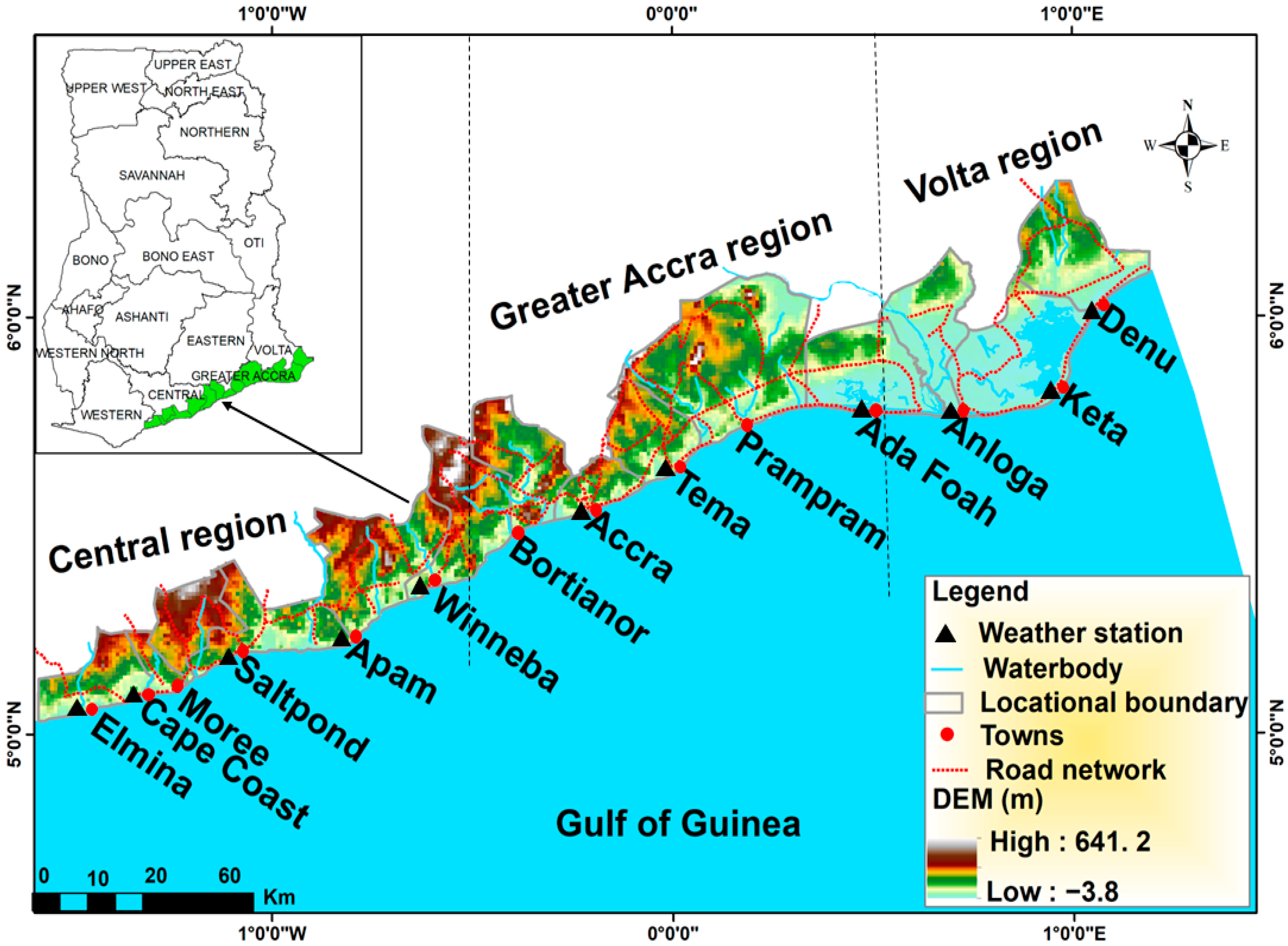
Here, we describe the methods and statistical measures used to analyze the extreme temperature and rainfall indices (Section 2.2) and future climate change projections (Section 2.3) in the zone.

2.1. Study Area

The coastal Savannah agroecological zone is one of the six agroecological zones located on the central and eastern coasts of Ghana (Figure 1). The zone is part of the central, Greater Accra, and Volta administrative regions of Ghana (Figure 1). The elevation of the zone ranges from the lowest point of −3.8 m from the coast to the highest point of 641.2 m inland (Figure 1). The zone has two rainfall seasons: the major, from April to July (with maximum rainfall in June), and the minor, from September to early November (with maximum rainfall in October) [72,73]. The dry season begins in late November and continues until March. Although the zone has a double maxima rainfall regime, it receives the least amount of rainfall out of the six agroecological zones in Ghana [73]. The average monthly temperature ranges from a minimum of 24.7 °C in August to a maximum of 32.7 °C in March [74]. Most of the zone’s vegetation is grassland, with few trees in the central portion and shrubs, thickets, and mangroves in the eastern portion [73]. Given its coastal nature, the zone makes a substantial contribution to Ghana’s gross domestic product [73]. Agriculture, fishing, tourism, trade, transportation, and services are the principal economic activities in the zone [72]. Among the major towns are Accra (the capital city), Cape Coast, Elmina, Moree, Saltpond, Apam, Winneba, Bortianor, Tema, Prampram, Ada Foah, Anloga, Keta, and Denu (Figure 1).

Table 1. Study locations, coordinates, and population. Source: Ghana Statistical Service (GSS) [73].

S/N	Location	Latitude	Longitude	Population
1	Accra	5° 60′ N	0° 18′ W	1,665,086
2	Ada Foah	5° 46′ N	0° 37′ E	71,671
3	Anloga	5° 47′ N	0° 53′ E	22,722
4	Apam	5° 17′ N	0° 44′ W	135,189
5	Bortianor	5° 30′ N	0° 20′ W	32,485
6	Cape Coast	5° 06′ N	1° 15′ W	169,894
7	Denu	6° 03′ N	1° 11′ E	160,756
8	Elmina	5° 05′ N	1° 20′ W	144,705
9	Keta	5° 45′ N	0° 30′ E	147,618
10	Moree	5° 07′ N	1° 12′ W	117,185
11	Prampram	5° 43′ N	0° 07′ E	14,897
12	Saltpond	5° 20′ N	1° 05′ W	144,332
13	Tema	5° 44′ N	0° 01′ E	402,637
14	Winneba	5° 21′ N	0° 37′ W	68,597

shows the coordinates and population of the major towns, which also served as the data stations for the study.

2.2. Data Sources and Methods of Analysis

2.2.1. Observed Data

Observed daily maximum (T_max) and minimum (T_min) temperature and rainfall data that spanned from 1981 to 2021 was obtained from the Ghana Meteorological Agency (GMet) and the National Aeronautics and Space Administration/Prediction of Worldwide Energy Resources (NASA/POWER). Data for 11 stations, including Accra, Ada Foah, Anloga, Apam, Cape Coast, Denu, Elmina, Keta, Saltpond, Tema, and Winneba, were provided by the GMet, while those of Moree, Bortianor, and Prampram were acquired from the NASA/POWER satellite data. The R-Instat software (version 0.70) was employed to check for missing gaps in the station data obtained from the GMet. Under this analysis, the number of missing gaps in each dataset was less than 2%. In developing nations, climate data quality is a major obstacle [44], and as reiterated by Wilby et al. [75], the regions most susceptible to climate variability also have the largest data gaps.

With less than 2% missing data in each dataset, the complete case analysis could have been an acceptable method [76]. However, we used multiple imputation by chained equations (MICE) to fill in the gaps. MICE was chosen because it has the capacity to fill in missing values in the original dataset by creating multiple missing values [77,78]. In this method, a prediction model is developed for the target attribute, and missing values are imputed based on the observed values for a particular station. Thus, missing values become indicative of the observed data. Recent research conducted by Abdullah et al. [79] demonstrates the suitability of the MICE approach. See Azur et al. [80] for more information about the MICE method, including the imputation procedure and relevant software.

2.2.2. Homogeneity Test and Homogenization

We utilized the RClimDex software (version 1.0) (http://etccdi.pacificclimate.org/software.shtml accessed on 15 September 2022) to examine each station’s daily T_max, T_min, and rainfall datasets for any anomalous values. Here, we first determined whether a situation existed in which the daily T_max was equal to or less than the T_min and rainfall was less than zero. Again, we highlighted outliers within four standard deviations in each of the datasets [81]. Additional evaluations were performed on the detected outliers to keep those that matched the value for a certain week or month. Without a suitable replacement for the highlighted values, we marked them as missing.

The RHtestsV4 package (http://etccdi.pacificclimate.org/software.shtml accessed on 15 September 2022) was further employed to check for homogeneity in the T_max and T_min datasets. So, the RHtestsV4 package made it possible to turn the daily T_max and T_min data into monthly datasets. During this phase, there were also a number of other steps, such as finding a reference dataset for the monthly T_max and T_min for homogenization, using the RHtests_dlyPrcp package (http://etccdi.pacificclimate.org/software.shtml accessed on 15 September 2022) for rainfall, and using the Quantile Matching (QM) adjustment method for the final homogenization.

According to Wang and Feng [82], a reference dataset is utilized to increase the precision of homogeneity analysis. Using the Penalized Maximal F (PMF) test, the homogeneity of the monthly T_max and T_min datasets from each of the 14 stations was evaluated [83,84]. This method is strongly advised for homogeneity analysis of reference datasets [82,85]. Through this analysis, it was determined that the Ada Foah station was homogeneous for both the T_max and T_min datasets; therefore, it was used as the reference series.

The Penalized Maximal t (PMT) test was then used to determine whether the monthly T_max and T_min datasets were homogeneous [83,84]. The base-minus-reference series was analyzed using this test to determine the significance and location of the changepoint and to develop a regression model to estimate the magnitude of the change [82]. Several research studies, such as works of [79,86,87], have demonstrated the superiority of the PMT test for inhomogeneity and changepoint analysis over other traditional approaches. Wang and Feng [82,85] have advised against using daily T_max and T_min datasets for PMT tests due to the noisy nature of daily time series and their computationally intensive nature, which may cause erroneous changepoint detection. Therefore, the monthly T_max and T_min datasets were utilized for the change point analysis. In addition, because the 14 stations lacked metadata that could have assisted us in analyzing the detected changepoints, we kept only Type-1 changepoints, which were significant even without metadata.

Due to the non-Gaussian and variable nature of rainfall [79], identifying an appropriate reference series is always a challenge [82,85]. For changepoint detection in rainfall datasets, the RHtests dlyPrcp package (http://etccdi.pacificclimate.org/software.shtml accessed on 15 September 2022) was used rather than the PMT test. According to Wang et al. [88], the RHtests dlyPrcp package converts a Box-Cox power transformation procedure into a common trend two-phase regression-model-based test that can detect changepoints in non-Gaussian datasets. Only the Type-1 changepoints were kept in this analysis.

Subsequently, the T_max, T_min, and rainfall datasets were homogenized with the use of the QM adjustment method. In this case, the QM adjustments for the various non-homogeneous datasets made use of the identified Type-1 changepoints. To make sure the QM adjustment process did not create any duplicated values, the homogenized datasets were again examined for unrealistic values. The outcome was a homogenized dataset in which the patterns of daily T_max, T_min, and rainfall data were consistent both prior to and after the changepoint analysis [88]. Wang et al. [88] went into greater detail about the QM adjustment process.

2.2.3. Calculation of Extreme Climate Indices

In this study, we utilized 23 out of the 27 ETCCDI variables (http://etccdi.pacificclimate.org/software.shtml accessed on 15 September 2022) to analyze extreme climatic events in the coastal Savannah agroecological zone of Ghana.

Table 2. Description and definition of climate indices.

Type	Indices	Description	Definition	Units
Temperature indices	TR20	Tropical nights	The annual count of days when daily minimum temperature is greater than 20 °C	Days
	CSDI	Cold spell duration index	A sequence of 6 or more days where daily minimum temperature is below the 10th percentile	Days
	WSDI	Warm spell duration index	A sequence of 6 or more days where daily maximum temperature is exceeds the 90th percentile	Days
	SU25	Summer days	The annual count of days where daily maximum temperature exceeds 25 °C	Days
	TNx	Max Tmin	Computes monthly or annual maximum of daily minimum temperature	°C
	TNn	Min Tmin	Computes monthly or annual minimum of daily minimum temperature	°C
	TN10p	Cool nights	Computes monthly or annual proportion of minimum temperature below 10th percentile	Days
	TN90p	Warm nights	Computes monthly or annual proportion of minimum temperature above 90th percentile	Days
	TXx	Max Tmax	Computes monthly or annual maximum of daily maximum temperature	°C
	TXn	Min Tmax	Computes monthly or annual minimum of daily maximum temperature	°C
	TX10p	Cool days	Computes monthly or annual proportion of maximum temperature below 10th percentile	Days
	TX90p	Warm days	Computes monthly or annual proportion of maximum temperature above 90th percentile	Days
	DTR	Diurnal temperature range	Computes the mean daily diurnal temperature range. The frequency of observation can either be monthly or annual	°C
Precipitation indices	R10	Number of heavy precipitation days	Computes the annual count of days where daily precipitation is more than 10 mm per day	Days
	R20	Number of very heavy precipitation days	Computes the annual count of days where daily precipitation is more than 20 mm per day	Days
	SDII	Simple precipitation index	Computes the annual sum of precipitation in wet days (days with precipitation over 1 mm) during the year divided by the number of wet days in the years	mm
	CDD	Consecutive dry days	Maximum number of days when precipitation is less than 1 mm	Days
	CWD	Consecutive wet days	Maximum number of days when precipitation is more than 1 mm	Days
	RX1day	Max 1-day precipitation amount	Computes monthly maximum 1-day precipitation	mm
	RX5day	Max 5-day precipitation amount	Computes monthly maximum consecutive 5-day precipitation	mm
	R95p	Very wet days	Computes the annual sum of precipitation in days where daily precipitation exceeds the 95th percentile	mm
	R99p	Extremely wet days	Computes the annual sum of precipitation in days where daily precipitation exceeds the 99th percentile	mm
	PRCPTOT	Annual total wet-day precipitation	Computes the annual sum of precipitation in wet days (days where precipitation is at least 1 mm)	mm

shows the list of the indices that were employed in this study. From Table 2, the 23 selected indices can be broadly grouped into absolute, percentile, and threshold categories [3,13]. The indices were calculated using 1981–2010 as the baseline period.

2.2.4. Trend Analysis

The Mann–Kendall (MK) test [89,90] was used to analyze trends in extreme climate indices, while Sen’s slope estimator was used to assess magnitudes of change [91]. The MK is a nonparametric test that compares the presence of a trend in a time series to the null hypothesis of no trend [92]. See da Silva et al.’s [92] work for more information on the MK test and Sen’s slope estimator. In this analysis, the Kendall tau statistic and its corresponding p-value were used to show the extent of the change, whether it was increasing or decreasing, and its significance. The MK test and Sen’s slope estimator were given confidence levels of 5% and 95% in this study, respectively. The MK test and Sen’s slope estimator were applied to the 14 individual stations first, then to the three regions (central, Greater Accra, and Volta), and finally to the entire zone (the average indices of all the 14 stations).

We looked at the seasonal variability of climate indices again over the last four decades (1981–1990, 1991–2000, 2001–2010, and 2011–2020). The year 2021 was excluded because including it would have added one more year to the last decade, given that the data period was 41 years long. Following the work of Abdullah et al. [79], we first examined the decadal variations of T_max, T_min, and rainfall for the three regions using a graphical representation. Following that, we used Welch’s two-sample t test (assuming unequal variance) to see if the mean changes between decades were statistically significant [79,93]. Furthermore, we examined the seasonal (wet, minor, and dry season) values for T_max, T_min, and rainfall in each decade for the three regions. Finally, we used the standardized anomaly to examine changes in climatic variables over the last several decades. Based on the study by Larbi et al. [35], we used the standardized anomaly computation shown below.

$$SA=\frac{\left(x-\mu \right)}{\sigma }$$

(1)

where x represents the seasonal value of the climatic variable, µ shows the long-term average, and σ indicates the standard deviation.

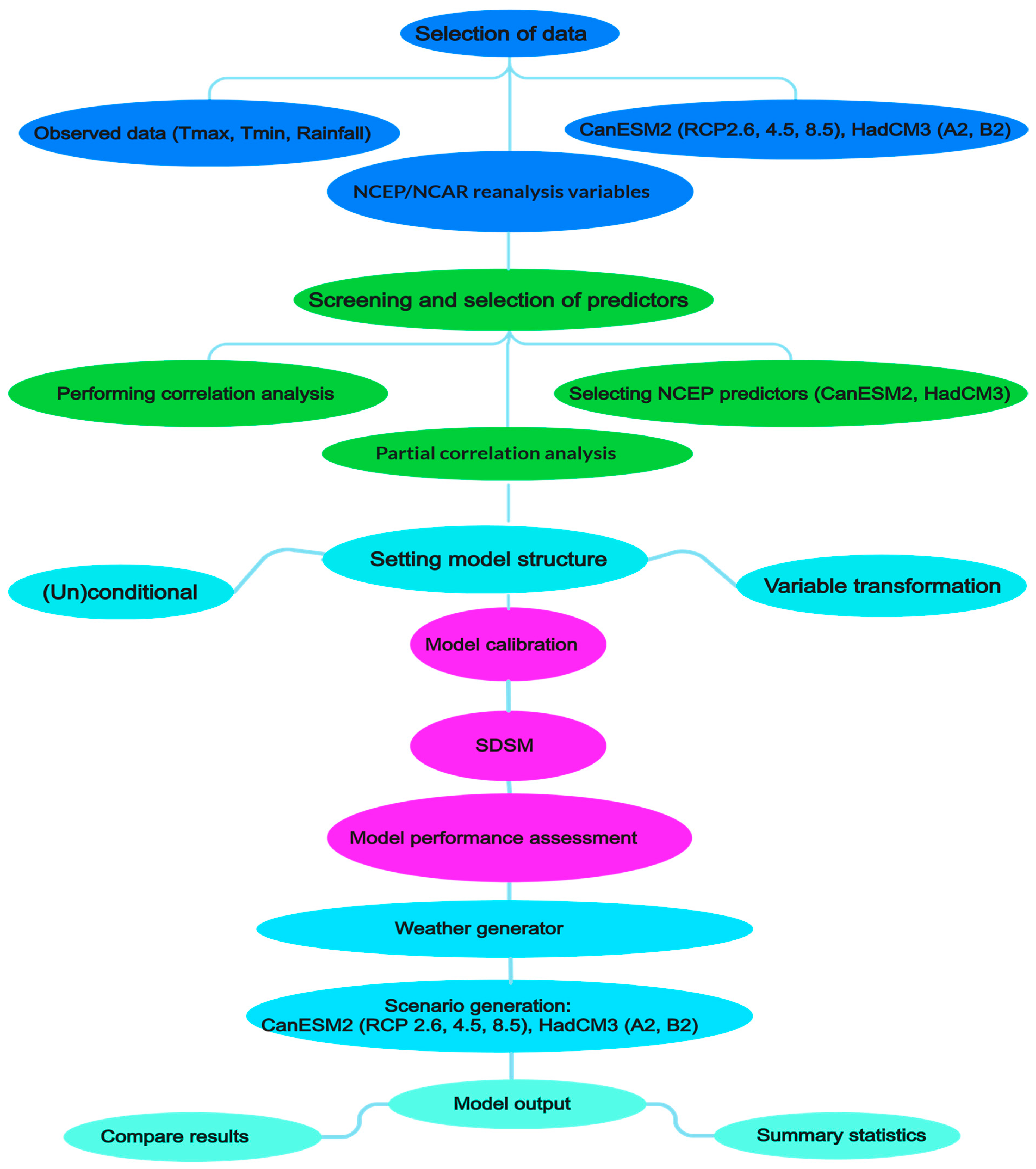
2.3. General Circulation Models (GCMs) Data

In addition to the observed daily data described in Section 2.2.1, we used 26 daily atmospheric reanalysis variables obtained from the National Center for Environmental Prediction/National Center for Atmospheric Research (NCEP/NCAR) for the periods 1961–2005 for the CanESM2 (https://climate-scenarios.canada.ca/?page=pred-canesm2 accessed on 17 September 2022) and 1961–2001 for the HadCM3 (https://climate-scenarios.canada.ca/?page=pred-hadcm3 accessed on 17 September 2022). Predictors are large-scale variables that are stored in GCM archives. The CanESM2 and HadCM3 NCEPs have spatial resolutions of 2.5° and 2.5°, respectively, with uniform longitude and latitude. The CanESM2 predictors for the central area are available in a GCM box (BOX_001X_34Y) and for Greater Accra and Volta (BOX_001X_35Y), while the HadCM3 predictors are available in a single GCM box (BOX_01X_30Y) for downscaling.

The CanESM2 and HadCM3 NCEPs are used for model calibration, while the predictors are used for validation and future projections. CanESM2 large-downscale predictor variables are available under the RCP2.6, RCP4.5, and RCP8.5 scenarios for future climate projections from 2006–2100, while HadCM3 large-downscale predictor variables are available under the A2 and B2 scenarios for future climate projections from 1961–2099. The study makes use of model data from Coupled Model Intercomparison Project phases 3 (CMIP3) and 5 (CMIP5). The principal interest is in assessing historical behavior and forecasting future coupled atmospheric-ocean general circulation models (AOGCMs). To generate future T_max, T_min, and rainfall, the statistical downscaling model (SDSM) was used. In analyzing the effects of climate change on climatic variables, the reference periods for the CanESM2 and HadCM3 are 1981–2010 and 1981–2006, respectively, while 2011–2100 and 2007–2099 are considered the future for the CanESM2 and HadCM3, in that order. Because their daily predictor variables are freely available to be inputted into the SDSM [56], the CanESM2 and HadCM3 GCMs were used in this study.

Table 3. CanESM2 and HadCM3 predictor variables used for downscaling.

	CanESM2		HadCM3
No.	Variable	Description	Variable	Description
1	mslp	Mean sea level pressure	mslp	Mean sea level pressure
2	p1_f	Surface airflow strength	p_f	Surface airflow strength
3	p1_u	Surface zonal velocity	p_u	Surface zonal velocity
4	p1_v	Surface meridional velocity	p_v	Surface meridional velocity
5	p1_z	Surface velocity	p_z	Surface velocity
6	p1th	Surface wind direction	p_th	Surface wind direction
7	p1zh	Surface divergence	p_zh	Surface divergence
8	p5_f	500 hPa airflow strength	p5_f	500 hPa airflow strength
9	p5_u	500 hPa zonal velocity	p5_u	500 hPa velocity
10	p5_v	500 hPa meridional velocity	p5_v	500 hPa meridional velocity
11	p5_z	500 hPa vorticity	p5_z	500 hPa vorticity
12	p500	500 hPa geopotential height	p500	500 hPa geopotential height
13	p5th	500 hPa wind direction	p5th	Mean sea level pressure
14	p5zh	500 hPa divergence	p5_zh	500 hPa divergence
15	p8_f	850 hPa airflow strength	p8_f	850 hPa airflow strength
16	p8_u	850 hPa zonal velocity	p8_u	850 hPa zonal velocity
17	p8_v	850 hPa meridional velocity	p8_v	850 hPa meridional velocity
18	p8_z	850 hPa vorticity	p8_z	850 hPa vorticity
19	p850	850 hPa geopotential height	p850	850 hPa geopotential height
20	p8th	850 hPa wind direction	p8th	850 hPa wind speed
21	p8zh	850 hPa divergence	p8zh	850 hPa divergence
22	prcp	Precipitation	r500	Relative humidity at 500 hPa
23	s500	Specific humidity at 500 hPa height	r850	Relative humidity at 850 hPa
24	s850	Specific humidity at 850 hPa height	rhum	Near surface relative humidity
25	shum	Surface specific humidity	Shum	850 hPa geopotential height
26	temp	Mean temperature at 2m	temp	Mean temperature

has a list of all 26 of the CanESM2 and HadCM3 daily predictor variables from NCEP.

2.3.1. Statistical Downscaling Model (SDSM)

Wilby et al. [94] created the SDSM by combining stochastic weather generators with multiple linear regression to construct local weather variables based on the statistical relationship between large-scale predictors and local climate variables. Regression-based downscaling is an established and often employed methodology [95]. The SDSM can downscale GCM outputs by establishing a statistical link between GCM variables (predictors) and local weather variables (predictands) using multiple linear regression models and stochastic bias-correction approaches [96]. To generate the daily local T_max, T_min, and rainfall using the SDSM, we used the CanESM2 acquired from the Canadian Center for Climate Modeling and Analysis as CMIP5 and the HadCM3 from the United Kingdom Hadley Centre as CMIP3, in addition to the NCEP data. Synthetic weather data were made using the CanESM2 RCP2.6, RCP4.5, and RCP8.5 scenarios from 2011–2100 and the HadCM3 A2 and B2 scenarios from 2007–2099.

The SDSM downscaling procedure includes the following steps: screening of predictor variables; model calibration; weather generation and generation of synthetic daily weather data; future ensemble data generation using predictor variables from the GCM; and summary statistics and results comparison for both observed and downscaled data [95,97]. Screening for significant predictors is an important step in statistical downscaling for model calibration in the SDSM [94]. Statistical methods are used to choose predictors, and at least two predictors are enough during the screening process [98].

To downscale the data from the given predictand and selected predictor variables, the calibration model was used in multiple regression equations. The model was designed to downscale T_max, T_min, and rainfall on a daily and monthly basis. The modeled data were adjusted to reflect the observed data using bias correction. The weather generator makes excellent use of independent data to validate the calibrated model. This procedure generates synthetic daily weather datasets for the specified period as well as a parameter file generated during the calibration stage using regression model weights. As a result, the SDSM provides a summary statistic that can be used to compare observed and modeled data. All 26 large-scale predictors from the NCEP were screened in this study, and the two that were found to be significant were used for model calibration.

The use of fewer predictors reduces computation time and improves the efficiency of the downscaling process [99]. The period for calibrating and validating the model between predictor and predictand data in the SDSM was divided into two parts: 1981–2010 and 1981–2006 for calibration, and 2011–2021 and 2007–2021 for validation of the CanESM2 and HadCM3 GCMs, respectively. The model was then used to generate future three-segment predictions for the 2030s (2011–2040), 2050s (2041–2070), and 2080s (2071–2100) for each GCM. A simplified representation of the SDSM is depicted in Figure 2. The mean of the generated scenarios was compared to the observed period, and the anomaly was revealed by the absolute difference in temperature and the percentage difference in rainfall from the monthly mean of the observed period to the future period. Positive and negative anomalies indicate an increase or decrease in the predictand in future periods. Using the calculations in Birara et al. [56], the following was carried out to figure out how T_max, T_min, and rainfall will change in the future:

$$\Delta P=\frac{\left(\mathit{Mm}·P-\mathit{Obs}·P\right)\times 100}{\mathit{Obs}·P}$$

(2)

$$\Delta T=\mathit{Mm}·T-\mathit{Obs}·T$$

(3)

where Mm·P and Mm·T show modeled rainfall and T_max or T_min, respectively, and Obs·P and Obs·T represent the observed rainfall and T_max or T_min, in that order.

2.3.2. Model Performance Assessment

A simulation of mean monthly T_max, T_min, and rainfall was checked during the calibration and validation of the downscale model using the coefficient of determination (R²), root mean square error (RMSE), and percent bias (PBIAS) expressed as:

To compare the explained variance of modeled data with the total variance of observed data, the coefficient of determination (R²) is required.

$${\mathrm{R}}^2=\frac{{{\displaystyle \sum }}_{i=1}^n{\left(y_i-\overline{x}\right)}^2}{{{\displaystyle \sum }}_{i=1}^n{\left(x_i-\overline{x}\right)}^2}$$

(4)

The RMSE expresses the difference between the modeled and observed values as follows:

$$\mathrm{RMSE}=\sqrt{\frac{{{\displaystyle \sum }}_{i=1}^n{\left(x_i-y_i\right)}^2}{n}}$$

(5)

$$\mathrm{PBIAS}=100\times \left[\frac{{{\displaystyle \sum }}_{i=1}^n\left(x_i-y_i\right)}{{{\displaystyle \sum }}_{i=1}^n\left(x_i\right)}\right]$$

(6)

where x_i and y_i are the observed and modeled data, respectively.

The R² has a value between 0 and 1. A value close to 1 indicates that the model fits the data perfectly. The better the model’s performance, the lower the RMSE. Using the PBIAS, it was determined whether the model underestimated or overestimated the observed data. The closer the PBIAS is to zero, the more precise the model.

3. Results

3.1. Results from Extreme Temperature and Rainfall Indices

3.1.1. Changepoints and Homogenization of Temperature and Rainfall

Table 4. Changepoints in temperature (maximum and minimum) and rainfall datasets.

Location	Tmax	Changepoints a	Tmin	Changepoints a	Rainfall	Changepoints b
Accra	0	−	3	31 December 1981, 31 November 1986, 31 January 1988	0	−
Ada Foah	Reference station
Anloga	0	−	0	−	0	−
Apam	1	31 September 2003	1	31 November 1986	0	−
Bortianor	1	31 September 2003	1	31 November 1986	0	−
Cape Coast	0	−	2	31 November 1981, 31 November 1986	0	−
Denu	0	−	0	−	0	−
Elmina	0	−	2	31 November 1981, 31 November 1986	0	−
Keta	0	−	0	−	0	−
Moree	0	−	2	31 November 1981, 31 November 1986	0	−
Prampram	0	−	3	31 December 1981, 31 November 1986, 31 January 1998	0	−
Saltpond	0	−	2	31 November 1981, 31 November 1986	0	−
Tema	0	−	3	31 December 1981, 31 November 1986, 31 January 1988	0	−
Winneba	1	31 September 2003	1	31 November 1986	0	−

^a Detected from monthly data; ^b Detected from daily data.

shows the changepoints in daily T_max and T_min and rainfall. Here, all the statistically significant changepoints are detected for the climatic variables. For T_max and T_min, the detected monthly changepoints were used to adjust the daily data. The monthly changepoints are converted to daily changepoints by transforming the preceding day of the identified month to a daily changepoint (see Section 2.2.2). From Table 4, changepoints for Apam, Bortianor, and Winneba were detected in October 2003. However, these were changed to 31 September 2003, to produce segments for homogenization during the QM adjustment. A similar situation occurred for T_min. For instance, in both Accra and Tema, the first changepoint appeared in January 1982, followed by December 1986 and February 1988. However, to produce segments, the detected changepoints were converted to 31 December 1981, 31 November 1986, and 31 January 1988, respectively.

Table 4 also shows no changepoints for rainfall across all the 14 locations and a few for T_max (Apam, Bortianor, and Winneba). However, more changepoints were observed for T_min at most locations, except Anloga, Denu, and Keta. These changepoints can be attributed to the abrupt daily temperature fluctuations at these locations.

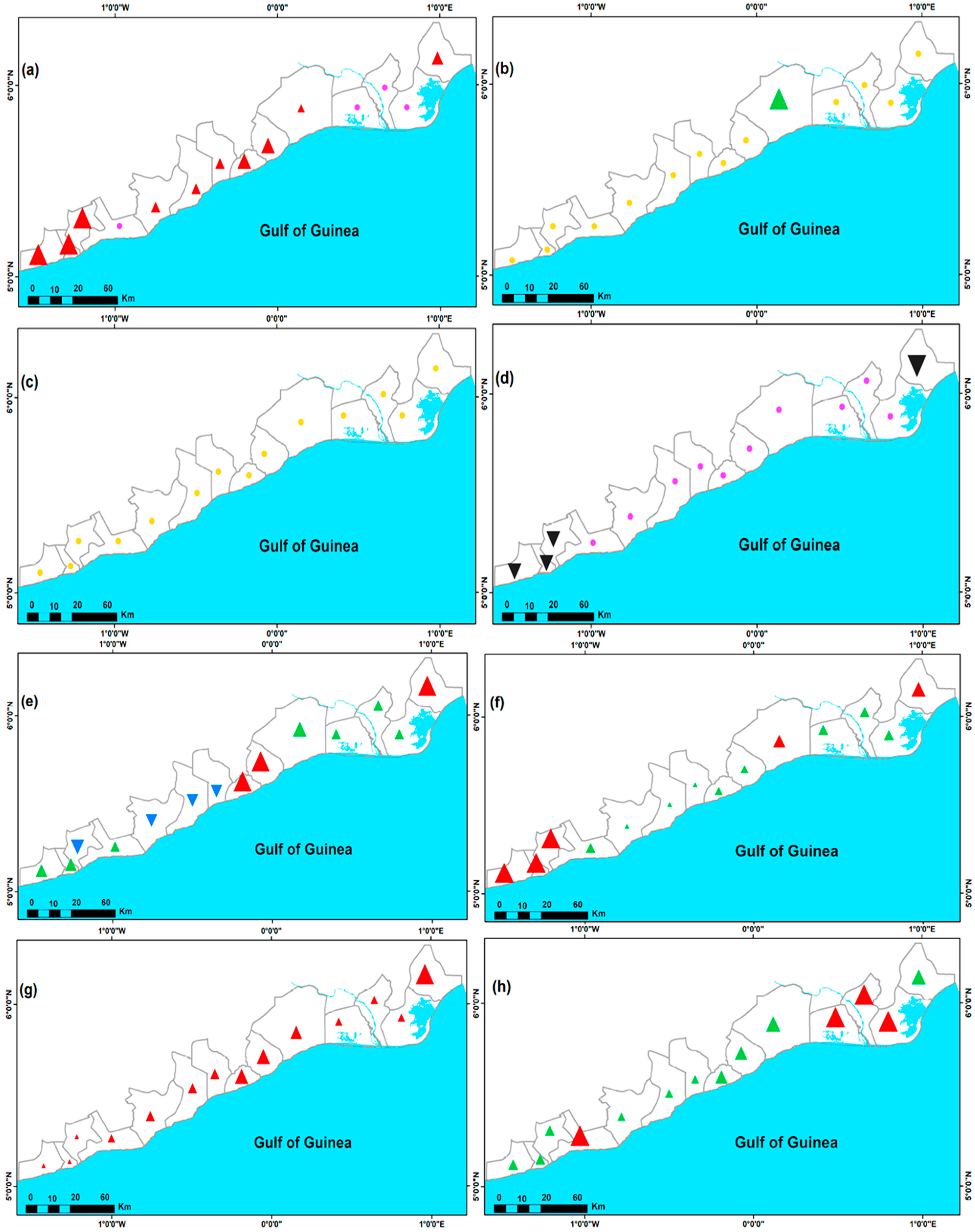
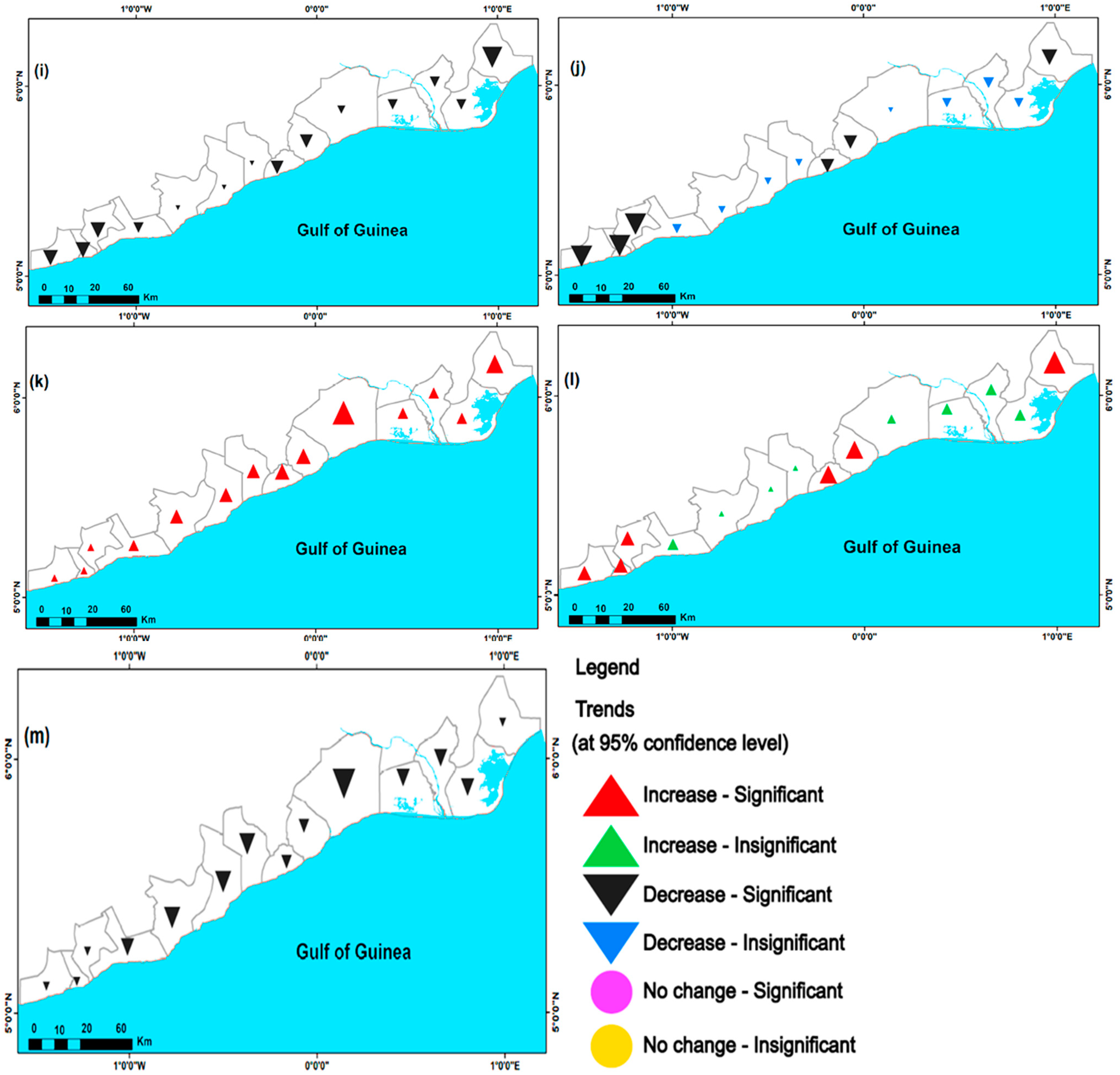
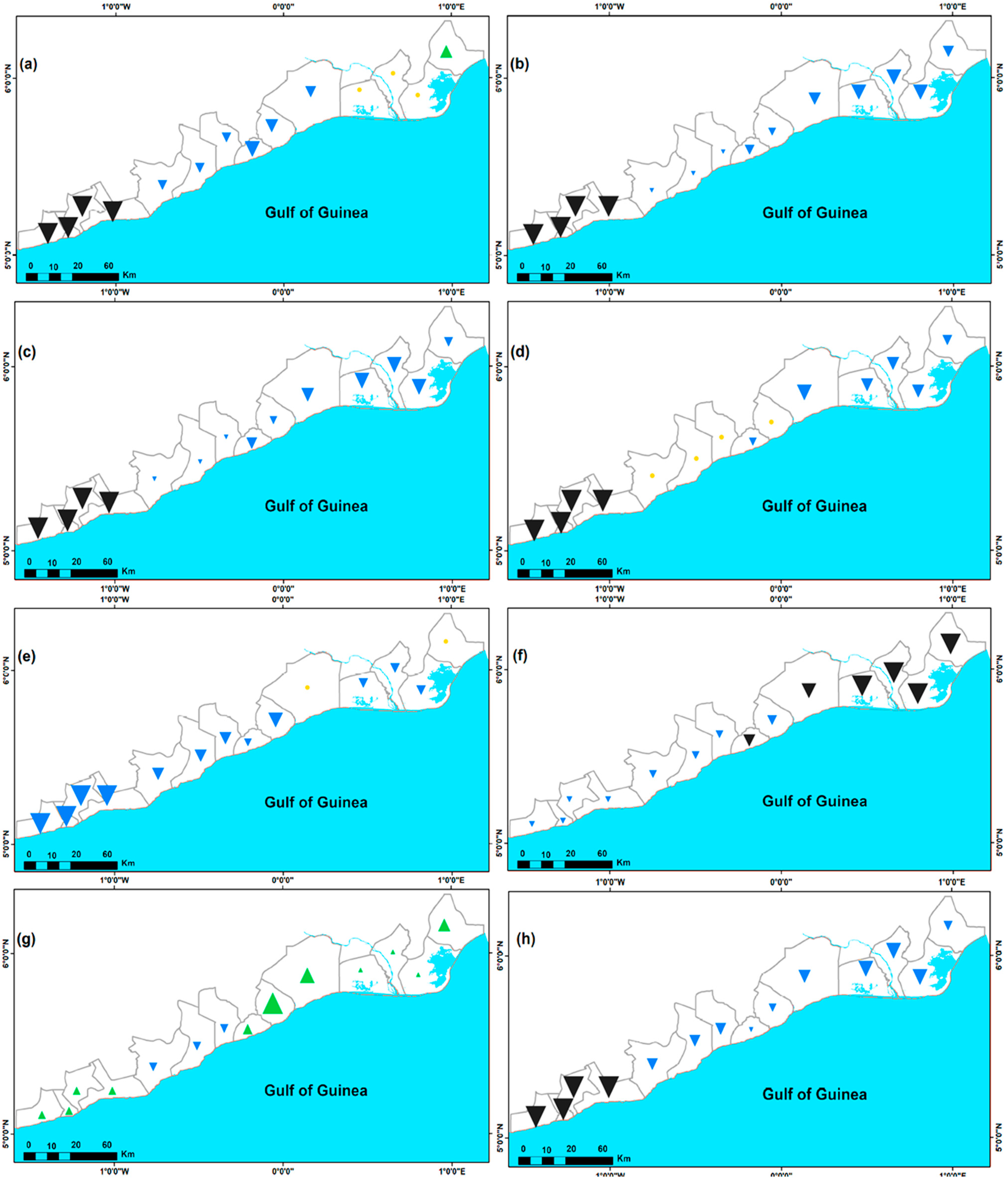
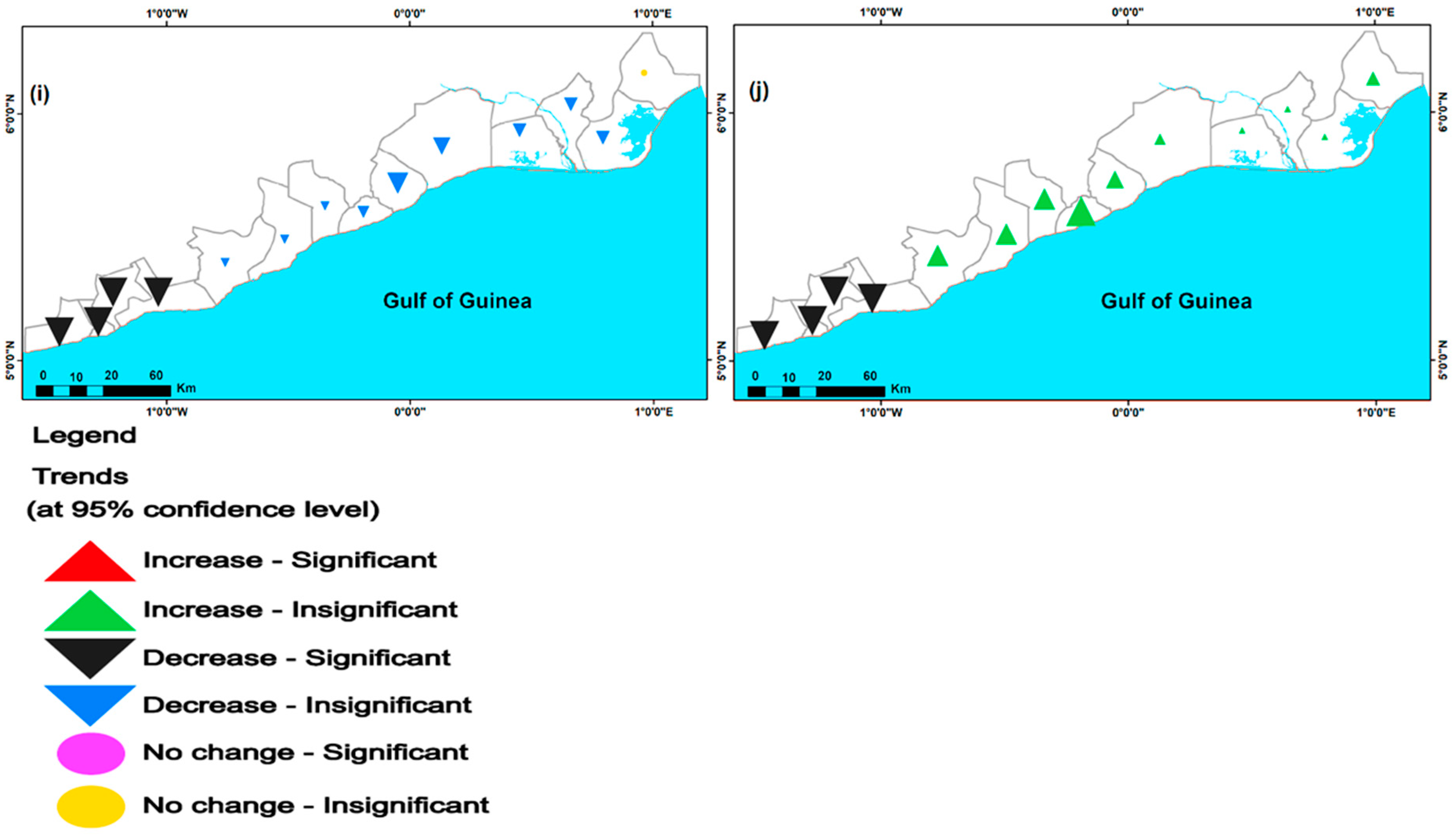
3.1.2. Extreme Temperature Indices

Table 5. Trends in extreme temperature indices for the coastal Savannah agroecological zone of Ghana.

Locations	SU25	TR20	WSDI	CSDI	TXx	TNx	TXn	TNn	TN10p	TX10p	TN90p	TX90p	DTR
Accra	0.231	0.000	0.000	0.000	0.014	0.008	0.033	0.016	−0.400	−0.220	0.383	0.217	−0.015
Ada Foah	0.000	0.000	0.000	0.000	0.003	0.010	0.026	0.026	−0.299	−0.113	0.376	0.104	−0.017
Anloga	0.000	0.000	0.000	0.000	0.003	0.010	0.026	0.026	−0.299	−0.116	0.376	0.104	−0.017
Apam	0.059	0.000	0.000	0.000	−0.004	0.007	0.030	0.008	−0.272	−0.041	0.378	0.020	−0.022
Bortianor	0.059	0.000	0.000	0.000	−0.004	0.007	0.030	0.008	−0.272	−0.041	0.378	0.020	−0.022
Cape Coast	0.571	0.000	0.000	−0.029	0.004	0.015	0.024	0.013	−0.409	−0.239	0.358	0.174	−0.012
Denu	0.167	0.000	0.000	−0.375	0.014	0.014	0.035	0.022	−0.432	−0.223	0.387	0.260	−0.012
Elmina	0.571	0.000	0.000	−0.029	0.004	0.015	0.024	0.013	−0.409	−0.239	0.358	0.174	−0.012
Keta	0.000	0.000	0.000	0.000	0.003	0.010	0.026	0.026	−0.299	−0.113	0.376	0.104	−0.017
Moree	0.571	0.000	0.000	−0.029	−0.008	0.015	0.024	0.013	−0.409	−0.239	0.358	0.174	−0.012
Prampram	0.053	0.056	0.000	0.000	0.008	0.013	0.032	0.022	−0.284	−0.037	0.399	0.058	−0.023
Saltpond	0.000	0.000	0.000	0.000	0.003	0.010	0.026	0.026	−0.299	−0.113	0.376	0.104	−0.017
Tema	0.231	0.000	0.000	0.000	0.014	0.008	0.033	0.016	−0.400	−0.220	0.383	0.217	−0.015
Winneba	0.059	0.000	0.000	0.000	−0.004	0.007	0.030	0.008	−0.272	−0.041	0.378	0.020	−0.022
Central region	0.290	0.000	0.000	−0.167	0.003	0.011	0.030	0.014	−0.335	−0.146	0.383	0.117	−0.016
Greater Accra region	0.000	0.016	0.000	−0.197	0.006	0.009	0.033	0.019	−0.332	−0.140	0.393	0.116	−0.019
Volta region	0.073	0.000	0.000	−0.233	0.007	0.012	0.029	0.024	−0.354	−0.142	0.393	0.156	−0.016
Entire zone (all locations)	0.176	0.006	0.000	−0.195	0.005	0.011	0.032	0.018	−0.346	−0.169	0.388	0.127	−0.018

Note: The values in the table are from the Sen’s slope estimator, which shows the magnitude of change per year. The values in bold are significant at 5% and 95% confidence levels, as observed from the MK test and Sen’s slope estimator, respectively. The values not in bold are insignificant at the same confidence level.

and Figure 3a–m show the long-term changes in extreme temperature indices and the spatial distribution of the trends in temperature for the coastal Savannah agroecological zone of Ghana. According to Table 5, the annual count of days where the daily temperature exceeded 25 °C (SU25) increased significantly for all locations, all regions, and for the entire zone during the analysis period. Figure 3a shows that while the trends SU25 increased for all locations, the magnitude of change is higher for the locations in the central region than for the remaining two regions (see Figure 1 to understand the regional divisions). Similar significant increases were observed for the monthly or annual minimum of the daily maximum temperature (TXn) and the proportion of warm nights (TN90p) across all locations, regions, and the entire zone. From Figure 3g,k, the magnitudes of changes in TXn and TN90p are higher in the Greater Accra region and some areas of the Volta region than in the central region. The proportion of cool nights (TN10p) and the diurnal temperature range (DTR) significantly decreased for all locations, regions, and the entire zone. Although the TN10p decreased significantly, the magnitude of the change was greater in the central region and some portions of the Volta region than in the Greater Accra region (Figure 3i), and the opposite occurred for the DTR (Figure 3m). Also, the cold spell duration indices (CDSI) significantly increased for the locations of Accra, Ada Foah, Anloga, Apam, Bortianor, Prampram, Saltpond, Tema, and Winneba, while a significant decrease ensued in Cape Coast, Denu, Elmina, and Moree (Figure 3d). Under the same analysis, all three regions and the entire zone decreased significantly.

The monthly or annual maximum of daily maximum temperature (TXx) (Figure 3e) significantly increased only for Accra, Denu, and Tema, whereas the monthly or annual maximum of daily minimum temperature (TNx) (Figure 3f) increased for Cape Coast, Denu, Elmina, Moree, Prampram, the central region, Volta region, and the entire zone. The monthly or annual minimum daily temperature (TNn) significantly increased in Ada Foah, Anloga, Keta, Saltpond, and the entire zone. Figure 3h reveals that the magnitude of change in TNn is higher in the Volta region and some areas of the central region than in the Greater Accra region. Moreover, the proportion of cool days (TX10p) significantly decreased for Accra, Cape Coast, Denu, Elmina, Moree, and Tema, and for the central and Volta regions and the entire zone, whereas the number of warm days (TX90p) significantly increased for Accra, Cape Coast, Denu, Elmina, Moree, and Tema, and the Greater Accra region. From Figure 3j, the decrease in TX10p is higher in the central region compared to that in the other two regions, while the magnitude of change in TX90p (Figure 3l) is higher in some portions of the Volta and Greater Accra regions.

3.1.3. Extreme Rainfall Indices

Table 6. Trends in extreme rainfall indices for the coastal Savannah agroecological zone of Ghana.

Locations	RX1day	RX5day	SDII	R10	R20	CDD	CWD	R95p	R99p	PRCPTOT
Accra	−0.105	−0.228	−0.011	−0.060	−0.029	−0.364	0.258	−1.086	−0.552	2.994
Ada Foah	0.000	−0.375	−0.016	−0.128	−0.030	−0.500	0.070	−2.099	−0.619	0.396
Anloga	0.000	−0.375	−0.016	−0.128	−0.030	−0.500	0.070	−2.099	−0.619	0.396
Apam	−0.058	−0.111	−0.002	0.000	−0.031	−0.123	−0.082	−1.649	−0.343	2.892
Bortianor	−0.058	−0.111	−0.002	0.000	−0.031	−0.123	−0.082	−1.649	−0.343	2.892
Cape Coast	−0.333	−0.895	−0.018	−0.279	−0.078	0.067	0.101	−4.500	−1.892	−3.694
Denu	0.016	−0.244	−0.010	−0.087	0.000	−0.500	0.282	−1.600	0.000	1.852
Elmina	−0.333	−0.895	−0.018	−0.279	−0.078	0.067	0.101	−4.500	−1.892	−3.694
Keta	0.000	−0.375	−0.016	−0.128	−0.030	−0.500	0.070	−2.099	−0.619	0.396
Moree	−0.333	−0.895	−0.018	−0.279	−0.078	0.067	0.101	−4.500	−1.892	−3.694
Prampram	−0.086	−0.250	−0.014	−0.164	0.000	−0.378	0.308	−2.000	−0.679	0.542
Saltpond	−0.333	−0.895	−0.018	−0.279	−0.078	0.067	0.101	−4.500	−1.892	−3.694
Tema	−0.098	−0.209	−0.004	0.000	−0.039	−0.143	0.449	−1.091	−1.225	2.496
Winneba	−0.058	−0.111	−0.002	0.000	−0.031	−0.123	−0.082	−1.649	−0.343	2.892
Central region	−0.248	−0.724	−0.013	−0.222	−0.082	0.000	−0.044	−3.967	−1.521	−2.049
Greater Accra region	−0.096	−0.199	−0.010	−0.083	−0.043	−0.294	0.218	−1.319	−1.000	1.654
Volta region	0.022	−0.272	−0.014	−0.102	−0.032	−0.500	0.195	−1.850	−1.850	1.161
Entire zone (all locations)	−0.127	−0.496	−0.026	−0.163	−0.077	−0.214	0.104	−2.759	−1.439	−0.758

Note: The values in the table are from the Sen’s slope estimator, which shows the magnitude of change per year. The values in bold are significant at 5% and 95% confidence levels, as observed from the MK test and Sen’s slope estimator, respectively. The values not in bold are insignificant at the same confidence level.

and Figure 4a–j show the long-term changes in extreme rainfall indices and the spatial distribution of the trends in rainfall for the coastal Savannah agroecological zone of Ghana. From Table 6, the maximum 1-day precipitation amount (RX1day) significantly decreased in Cape Coast, Elmina, Moree, and Saltpond. A similar and significant decrease, including in the central region, is observed in the maximum 5-day precipitation amount (RX5day). The simple precipitation index (SDII) significantly decreased in Cape Coast, Elmina, Moree, and Saltpond. The number of days of heavy precipitation (R10) also decreased significantly in Cape Coast, Elmina, Moree, and Saltpond. From Figure 4a–d, the magnitudes of changes in RX1day, RX5day, SDII, and R10 are greater in some areas of the central region than in the other two. The number of consecutive dry days (CDD) decreased significantly in Accra, Ada Foah, Anloga, Denu, Keta, Prampram, the Greater Accra and Volta regions, and the entire zone. That is, the Greater Accra and the Volta regions recorded more dry days than the central region (Figure 4f). The annual sum of very wet days (R95p) significantly decreased in Cape Coast, Elmina, Moree, Saltpond, and the central region. As shown in Figure 4h, the R95p in the central region is significantly lower than in the other two regions. A similar trend is observed in the annual sum of extremely wet days (R99p) (Figure 4i). From Table 6, both increasing and decreasing trends are observed for the consecutive wet days (CWD) and the annual total of wet-day precipitation (PRCPTOT). However, the trends were insignificant. This is also evident in Figure 4g,j.

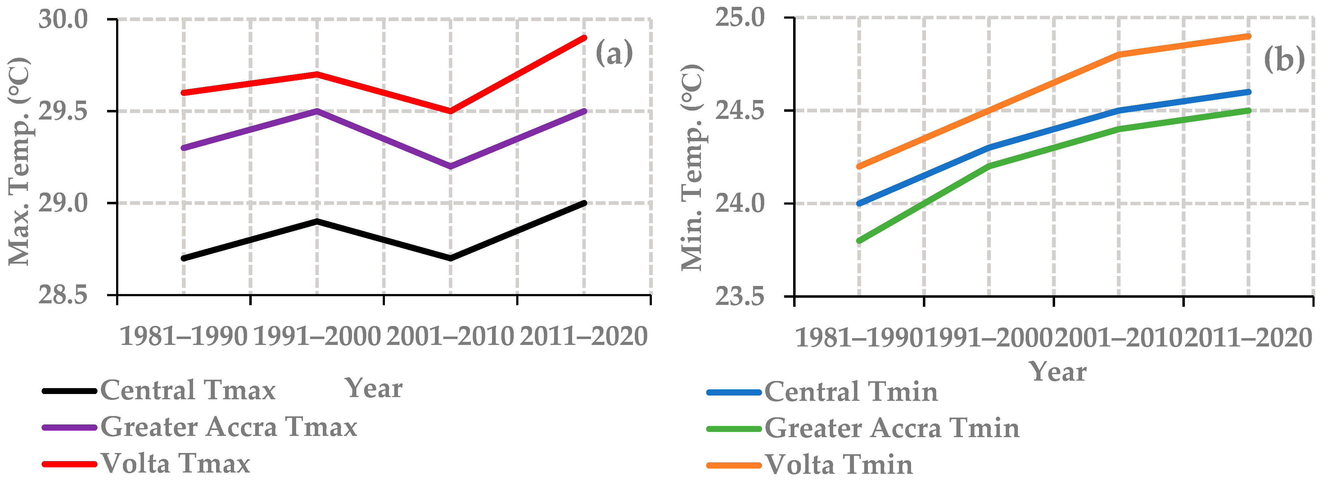
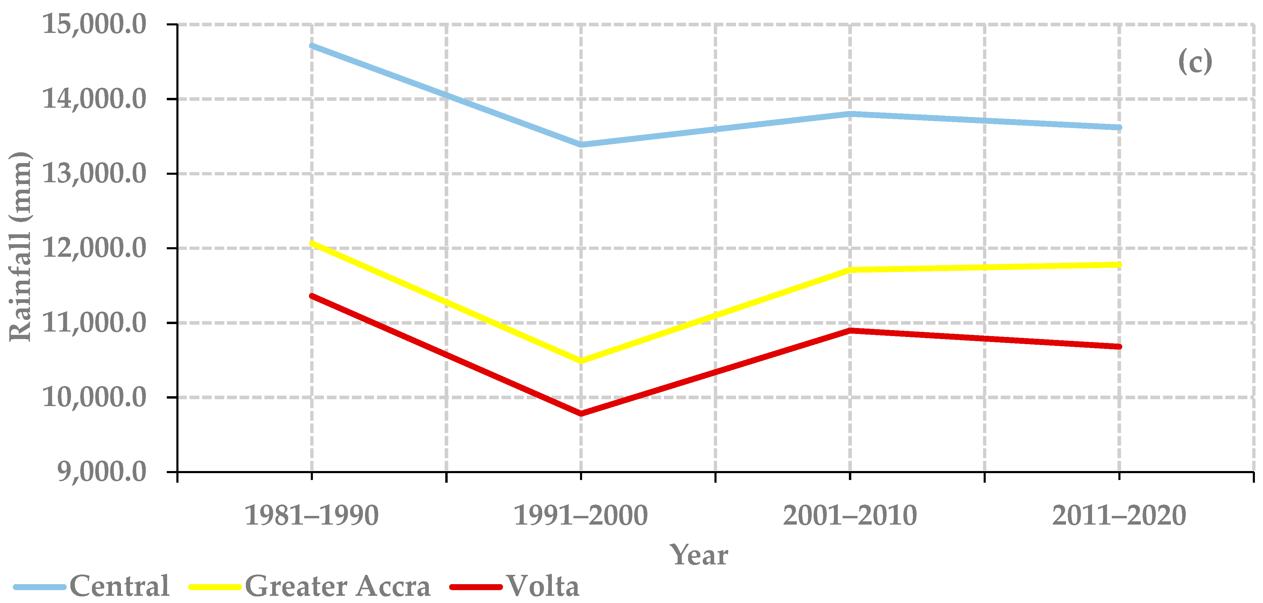
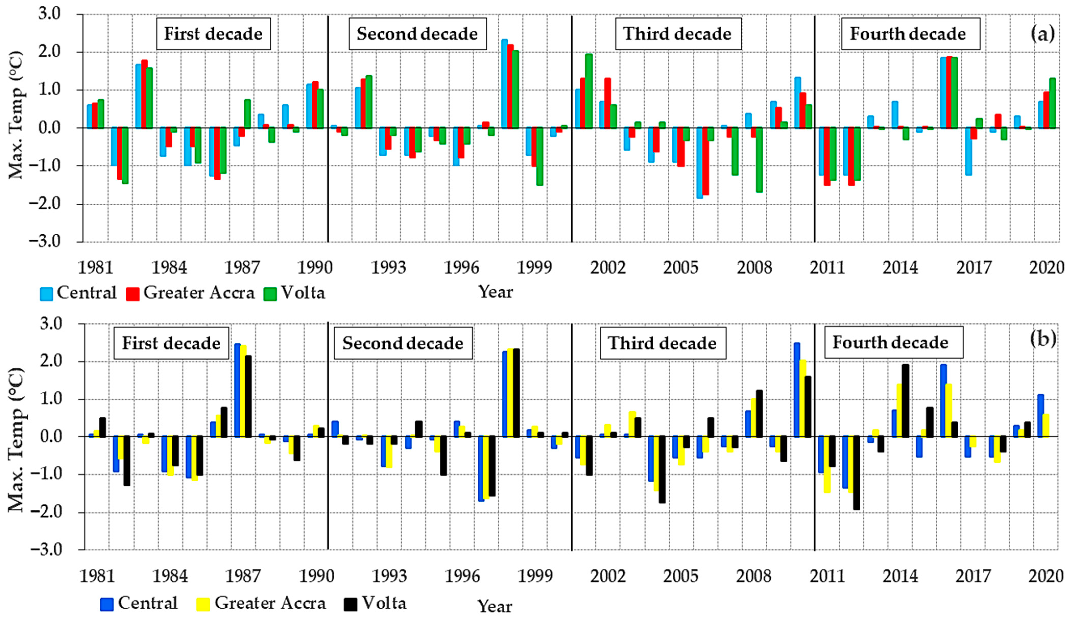
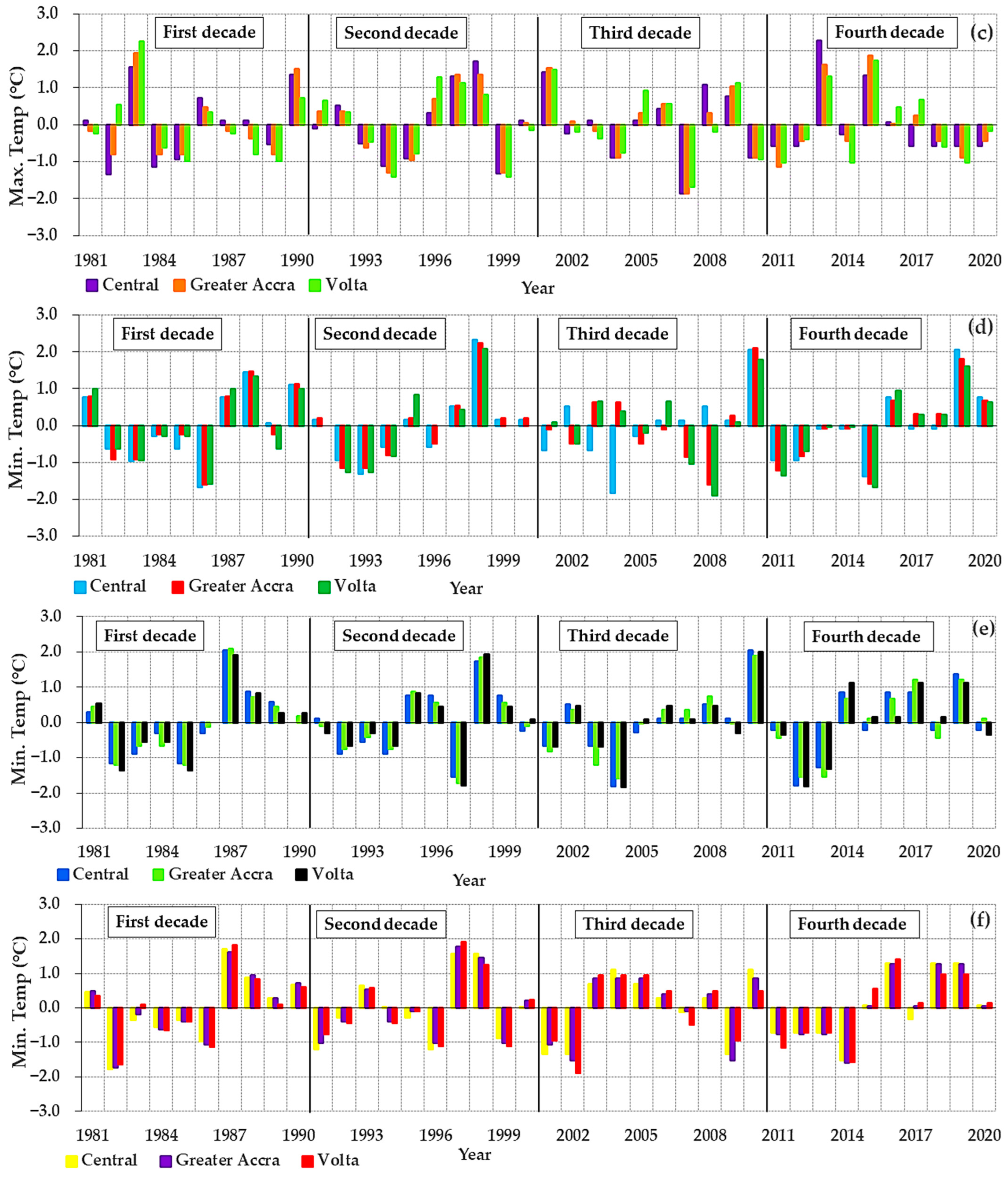
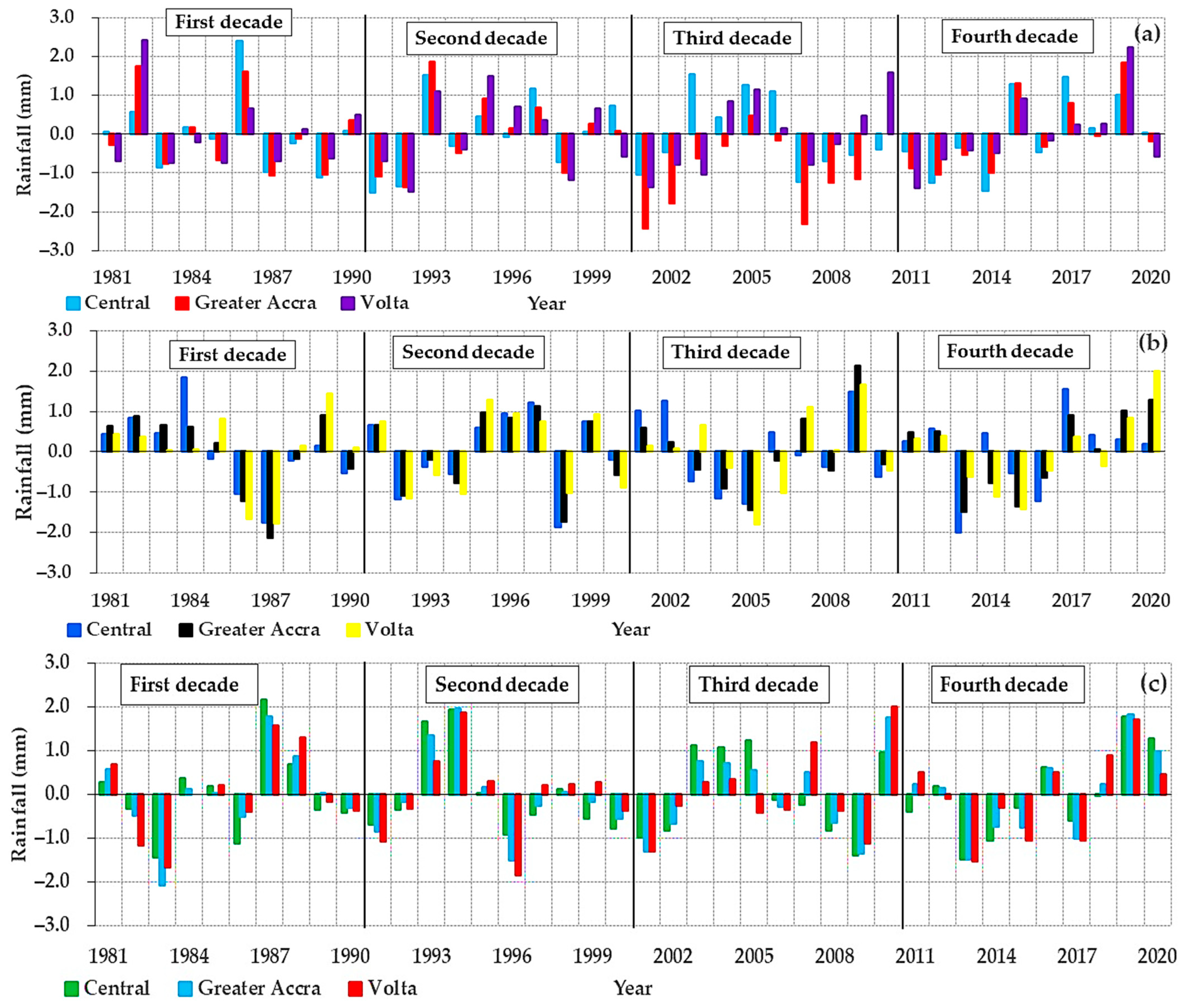
3.1.4. Decadal Variations in Temperature and Rainfall

Figure 5a–c depict the average daily maximum (T_max) and minimum (T_min) temperatures and rainfall in the coastal Savannah agroecological zone of Ghana over the last four decades. The results of Welch’s two-sample t test comparing the mean changes between decades for T_max, T_max, and rainfall in the central, Greater Accra, and Volta regions are presented in

Table 7. Results of the Welch’s t test analysis.

	Central			Greater Accra			Volta
	T Stat	p-Value	Sig.	T Stat	p-Value	Sig.	T Stat	p-Value	Sig.
First- and second-decades Tmax	−3.128	0.002	*	−3.306	0.000	*	−2.328	0.002	*
Second- and third-decades Tmax	4.216	2.518	−	6.372	1.972	−	5.055	4.404	−
Third- and fourth-decades Tmax	−6.572	5.286	−	−7.966	1.890	−	−9.244	3.063	−
First- and second-decades Tmin	−10.176	3.662	−	−10.706	1.497	−	−9.572	1.404	−
Second- and third-decades Tmin	−8.544	1.554	−	−7.436	1.155	−	−7.565	4.346	−
Third- and fourth-decades Tmin	−2.177	0.029	*	−3.130	0.002	*	−4.111	3.976	−
First- and second-decades rainfall	2.896	0.004	*	4.189	2.835	−	0.727	0.467	−
Second- and third-decades rainfall	2.896	0.004	*	−3.713	0.000	*	−3.713	0.000	*
Third- and fourth-decades rainfall	0.471	0.638	−	−0.190	0.849	−	4.135	3.594	−

* Shows significance at 95% confidence level, − indicates insignificance at 95% confidence level.

. Figure 6a–f and Figure 7a–c depict the standardized anomalies of T_max and T_min and rainfall, relative to the 1981–2020 mean. Based on Figure 5a, the decadal variability of T_max is greatest in the Volta region, followed by the Greater Accra region, and the central region has the lowest variability. T_max increased substantially in the first (1981–1990), second (1991–2000), and fourth (2011–2020) decades but decreased in the third (2001–2010). The T_min increased considerably across all regions and in each decade. Notwithstanding, the Volta region experienced a larger increase compared to the other two regions (Figure 5b). From Table 7, the Welch’s t test showed that T_max decreased significantly only between the first and second decades in all three regions, while T_min decreased significantly between the third and fourth decades in the central and Greater Accra regions.

Figure 5c shows that rainfall exhibits decadal variations. Rainfall increased in the first and third decades across all three regions but decreased in the second and fourth decades, except for Greater Accra, where it increased in the fourth decade. Based on Welch’s t test in Table 7, the central region had a significant increase in rainfall between the first and second decades. Between the second and third decades, the central region experienced a significant increase, while the Greater Accra and Volta regions observed significant decreases.

Generally, the anomalies in T_max and T_min show a stronger seasonal decadal variation across the zone (Figure 6a–f). Between 1981 and 2020, the highest positive (2.3) and negative (−1.8) dry season anomalies for T_max (Figure 6a) both occurred in the central region in the years of 1998 (the second decade) and 2006 (the third decade), respectively. In Figure 6b, the greatest positive (2.5) and negative (−1.9) wet season anomalies appeared in the central region and the Volta regions in 1987/2010 (both the first and third decades) and 2012 (the fourth decade), respectively. For the minor season (Figure 6c), the highest positive (2.3) occurred in the central region in 2013 (the fourth decade), while the highest negative (−1.9) ensued in the same region and the Greater Accra region in 2007 (the third decade).

From Figure 6d, the greatest positive (2.3) and negative (−1.9) anomalies for the dry season T_min occurred in the central and Volta regions in 1998 (the second decade) and 2008 (the third decade), respectively. For the wet season (Figure 6e), the greatest positive (2.1) ensued in both the central and Greater Accra regions in 1987/2010 (both the first and third decades), while the greatest negative (−1.8) appeared in the central and Volta regions in 2004 (the third decade). In Figure 6f, the highest positive (1.9) and negative (−1.9) anomalies for T_min were both recorded in the Volta region in the years 1997 (second decade) and 2002 (third decade), respectively.

The anomalies in the mean decadal seasonal rainfall (Figure 7a–c) indicate greater improvements in the wet and minor seasons than in the dry season, despite variations. Between 1981 and 2020, the Volta and central regions recorded the highest positive (2.4) dry season rainfall in the years of 1982 and 1986, respectively, both occurring in the first decade, while the highest negative (−2.4) rainfall appeared in the Greater Accra region in 2001 (the third decade) (Figure 7a). For the wet season (Figure 7b), both the greatest negative (−2.1) and positive (2.1) rainfall anomalies ensued in the Greater Accra region in 1987 (the first decade) and 2009 (the third decade), in that order. According to Figure 7c, the Greater Accra and the central regions experienced the highest negative (−2.1) and positive (2.1) minor season rainfall anomalies in the years 1983 and 1987, respectively, both occurring in the first decade.

3.2. Results for Future Climate Change Projection

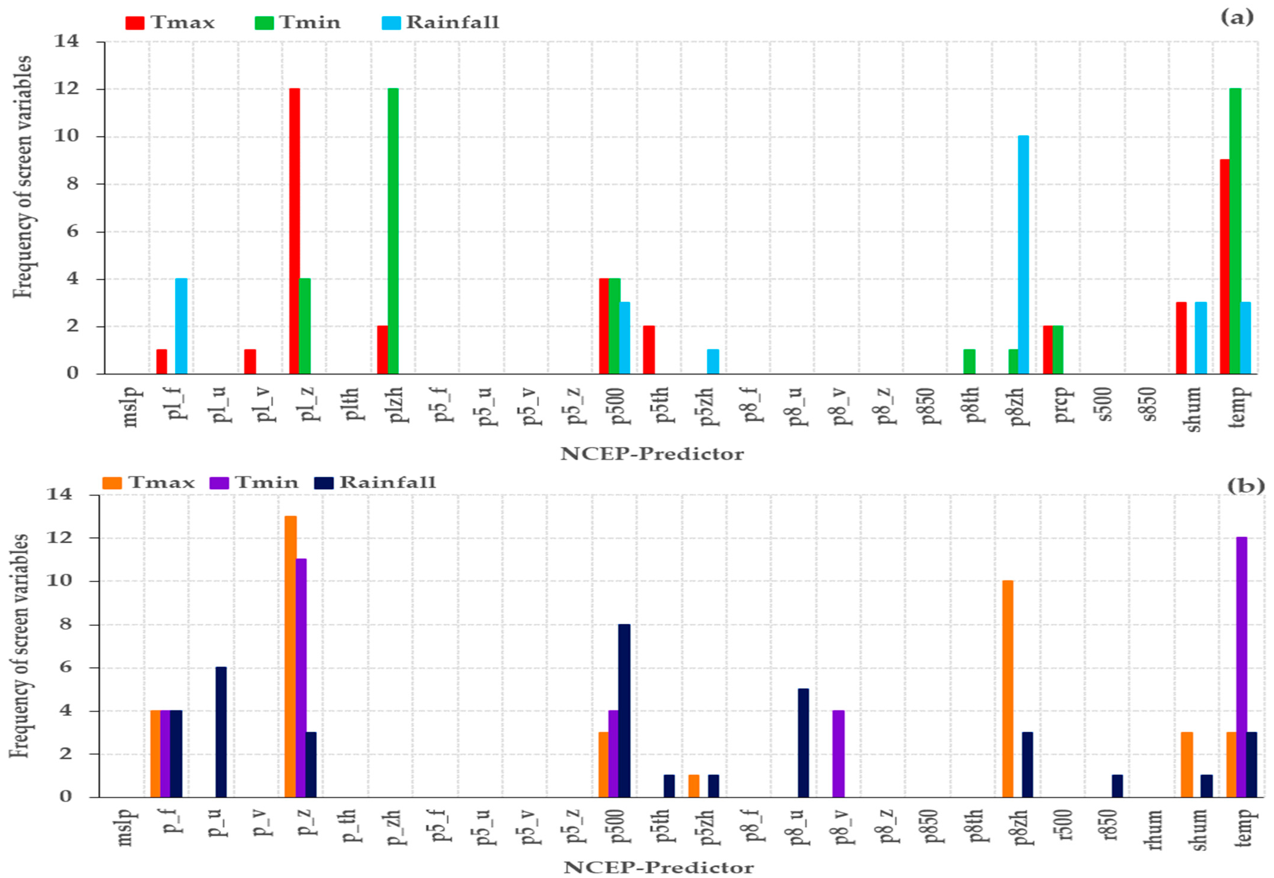
3.2.1. Predictor Variables Selection

The selection of appropriate predictor variables is essential to the success of the SDSM method. A correlation matrix between the individual predictand and the NCEP variables was used to screen the appropriate predictors. The 26 large-scale daily predictors from the NCEP reanalysis were utilized together with the predictors with the highest correlation coefficient from the individual predictands (T_max, T_min, and rainfall) for all three regions (i.e., central, Greater Accra, and Volta). Figure 8a,b shows a summary of the screened variables of the NCEP predictors. Figure 8a shows that the pl_z, plzh, and temp, and p8zh, correlated well to predict T_max, T_min, and rainfall for the CanESM2. The p_z, temp, and p500 also correlated well with T_max, T_min, and rainfall in that order for the HadCM3 (Figure 8b). It can be said that the individual predictor variables identified for the CanESM2 and HadCM3 GCMs are controlled by different local variables in each region. Again, it can be said that surface velocities (pl_z and p_z) and mean temperature at 2 m (temp) served as potential predictors of temperature (T_max and T_min) for all the regions.

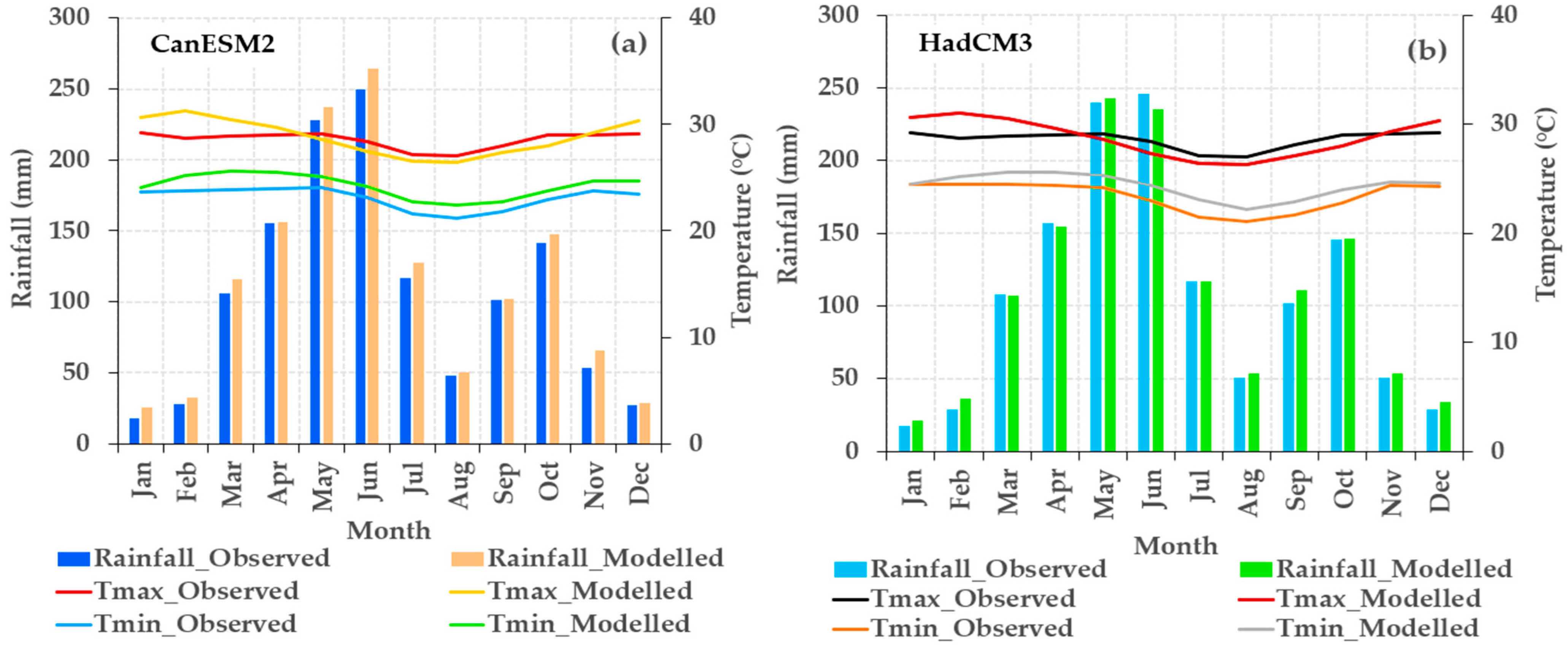
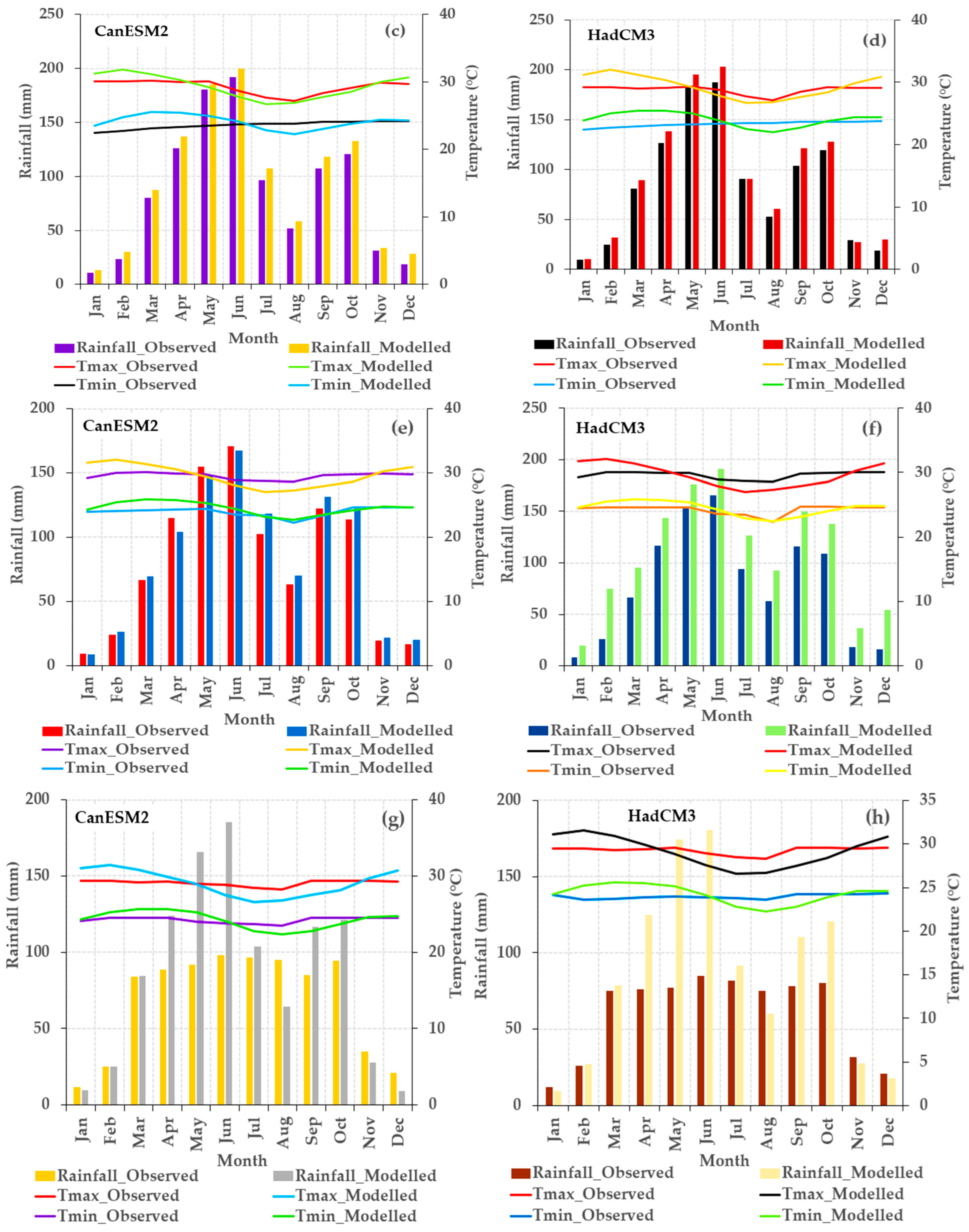
3.2.2. Model Performance Assessment during Calibration and Validation

The study used calibration periods of 30 (1981–2010) and 26 (1981–2006) years and validation periods of 11 (2011–2021) and 15 (2007–2021) years for CanESM2 and HadCM3, respectively. The statistical performance regarding the coefficient of determination (R²), the root mean square error (RMSE), and the percent bias (PBIAS) of the model is also presented in

Table 8. Statistical performance during calibration and validation for Tmax, Tmin, and rainfall.

Predictand	Area		CanESM2			HadCM3
			R2	RMSE	PBIAS	R2	RMSE	PBIAS
Tmax	Central region	Calibration	0.95	0.01	−0.22	0.79	0.10	0.01
		Validation	0.82	0.20	0.34	0.68	0.32	−0.42
	Greater Accra region	Calibration	0.99	0.22	0.11	0.99	0.33	0.23
		Validation	0.91	0.41	−0.23	0.98	0.56	−0.32
	Volta region	Calibration	0.99	0.02	0.02	0.99	0.11	0.01
		Validation	0.79	0.31	0.34	0.77	0.21	0.23
	Entire zone	Calibration	0.99	0.20	0.11	0.96	0.10	0.11
		Validation	0.87	0.31	0.23	0.86	0.32	0.31
Tmin	Central region	Calibration	0.99	0.01	0.02	0.98	0.02	0.01
		Validation	0.91	0.32	0.11	0.88	0.52	0.40
	Greater Accra region	Calibration	0.99	0.21	0.23	0.99	0.12	0.21
		Validation	0.87	0.44	1.13	0.89	0.91	0.52
	Volta region	Calibration	0.99	0.03	0.02	0.99	0.13	0.02
		Validation	0.94	0.52	0.31	0.79	0.31	0.70
	Entire zone	Calibration	0.99	0.21	0.22	0.99	0.05	0.20
		Validation	0.91	0.42	0.31	0.89	0.23	0.61
Rainfall	Central region	Calibration	0.99	0.54	5.44	0.89	0.61	6.02
		Validation	0.76	0.63	6.03	0.77	0.80	7.22
	Greater Accra region	Calibration	0.95	0.82	4.01	0.89	0.81	4.41
		Validation	0.91	1.02	7.11	0.79	0.90	6.32
	Volta region	Calibration	0.92	0.42	4.12	0.88	0.40	7.01
		Validation	0.79	0.55	6.23	0.58	0.61	9.15
	Entire zone	Calibration	0.99	0.54	7.34	0.99	0.90	7.89
		Validation	0.76	0.63	10.01	0.89	0.81	11.79

. The CanESM2 and HadCM3 models’ performances were good and ranged from 58–99%, 0.01–1.02 °C, and 0.42–11.79 °C, respectively, for R², RMSE, and PBIAS (for all three regions and the entire zone) (Table 8). The performance of CanESM2 ranged from 76–99%, 0.01–1.02 °C, and 0.22–10.01 °C for R², RMSE, and PBIAS, respectively. The performance of the HadCM3 also ranged from 58–99%, 0.02-0.91 °C, and 0.42–11.79 °C for R², RMSE, and PBIAS, in that order.

Table 8 shows low performance for rainfall as compared to the T_max and T_max, especially during validation under both models. Figure 9a–h show the graphical representation of the results of the model calibration and validation for the central region (Figure 9a,b), the Greater Accra region (Figure 9c,d), the Volta region (Figure 9e,f), and the entire zone (Figure 9g,h). The low performance could be attributed to the conditional modeling behavior of rainfall and the difficulty of achieving a perfect multiple regression in the SDSM. Regarding model comparison, the CanESM2 outperformed the HadCM3 during both calibration and validation, especially for rainfall in all three regions and the entire zone (Table 8). Notwithstanding, both models performed better for T_max and T_min.

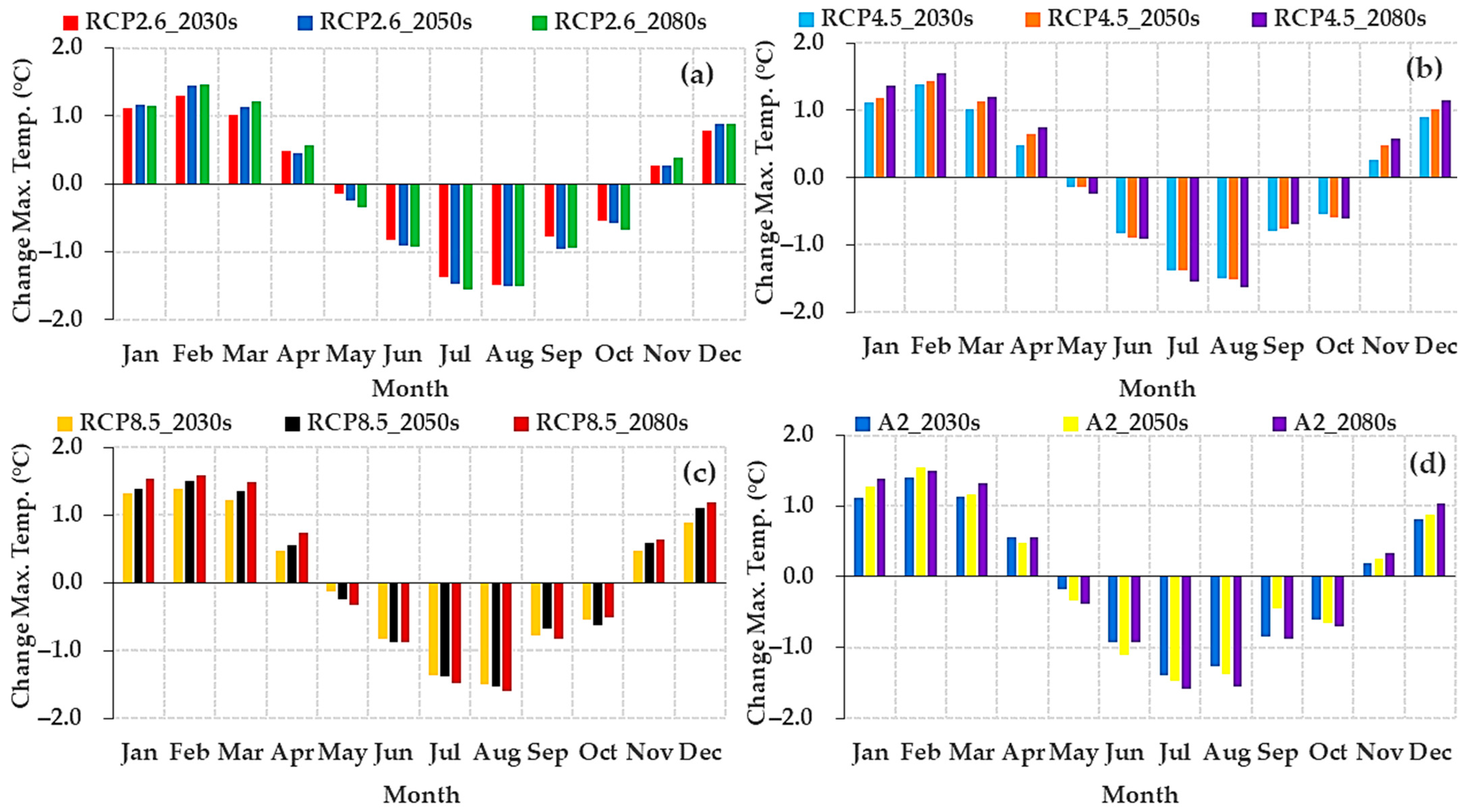
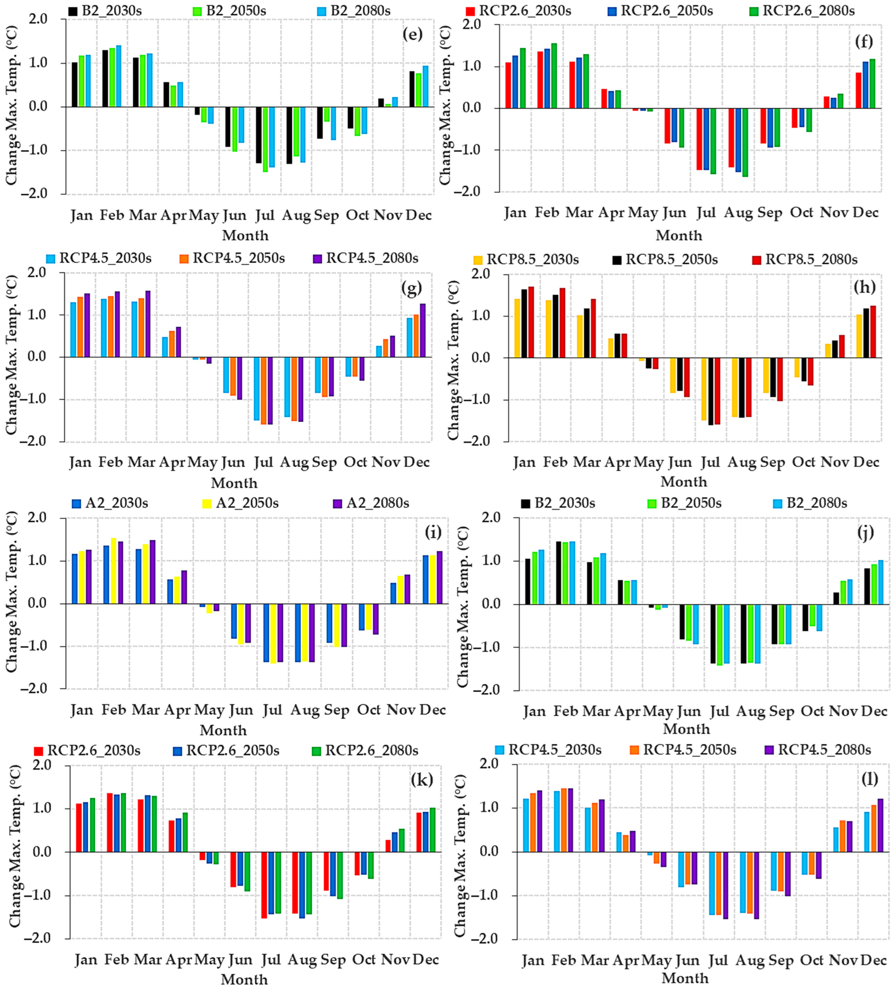
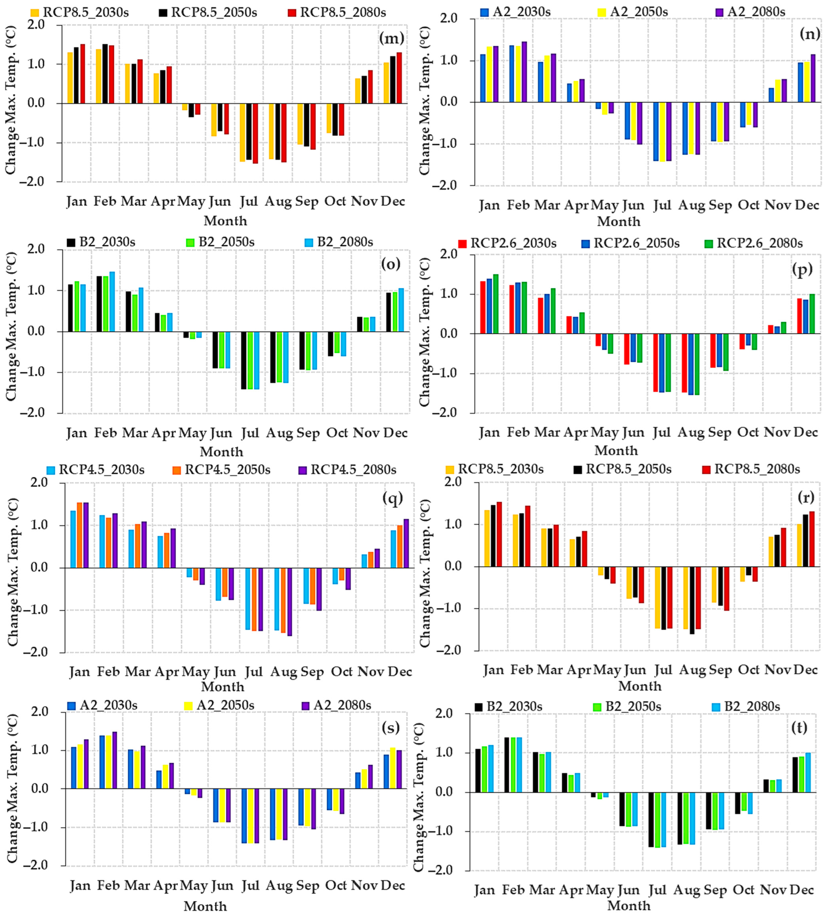
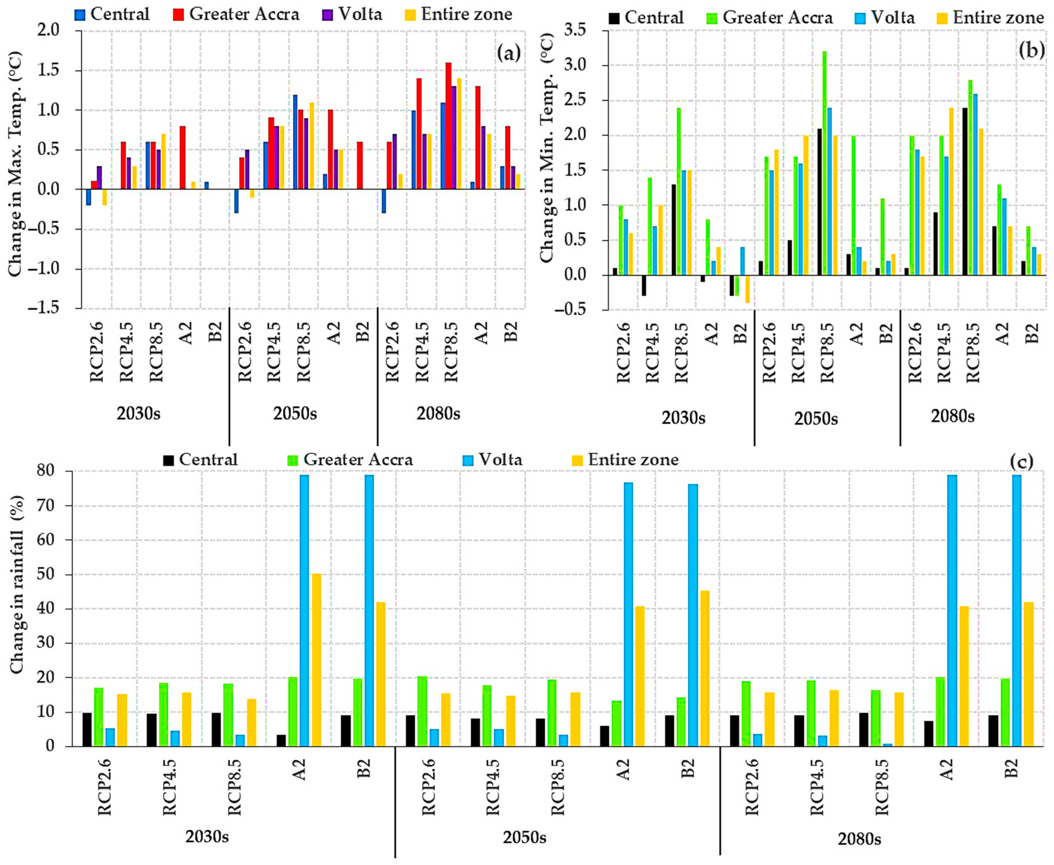
3.2.3. Change in Projected Future Monthly Maximum Temperature (T_max)

Figure 10a–t depict the projected future monthly T_max change for the central region (Figure 10a–e), Greater Accra region (Figure 10f–j), Volta region (Figure 10k–o), and entire zone (Figure 10p–t) using the CanESM2 (RCP2.6, 4.5, and 8.5) and HadCM3 (A2 and B2) models for the 2030s, 2050s, and 2080s. The overall results from the scenarios generated from the CanESM2 and HadCM3 models reveal that T_max will increase in most months for the 2030s, 2050s, and 2080s for all three regions and across the entire zone (Figure 10a–t). The A2 scenario reveals a higher projection for T_max than the B2 scenario for the regions and the entire zone (Figure 10d,e,i,j,n,o,s,t). Under the RCP2.6, 4.5, and 8.5 scenarios, T_max is projected to increase largely in all three regions and for the entire zone. In comparison to the RCP scenarios, T_max shows a greater projected increase for RCP8.5 than the other two scenarios (Figure 10a–c,f–h,k–m,p–r).

In both models and scenarios, a clear seasonal variation can be observed in the projected T_max. In the future, T_max will increase greatly in the dry season (November–March) and decrease substantially in the wet (May–July) and minor (September–October) seasons (Figure 10a–t). T_max is expected to increase significantly more in Greater Accra (Figure 10f–j) and Volta (Figure 10k–o) than in the central region (Figure 10a–e). Moreover, among the years, T_max is expected to increase considerably more in the 2050s and 2080s than in the 2030s. Regardless, greater variation in T_max is observed in all scenarios for the 2080s. T_max is expected to be highest (1.6 °C) and lowest (−1.6 °C) across the three regions (Figure 11a–o), as well as highest (1.5 °C) and lowest (−1.6 °C) for the entire zone (Figure 11p–t). In comparing the two models, the RCPs outperformed the A2 and B2 scenarios.

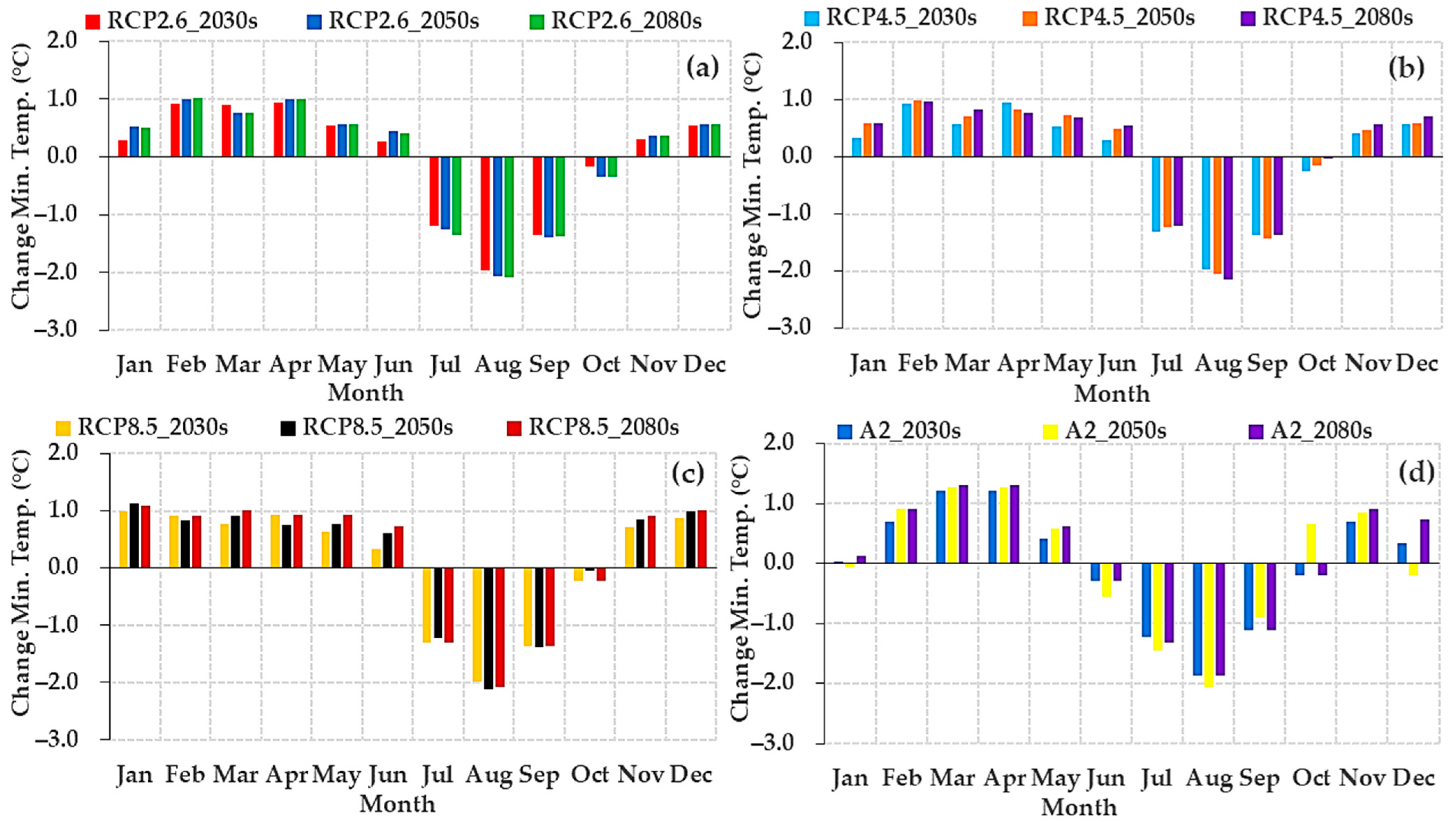
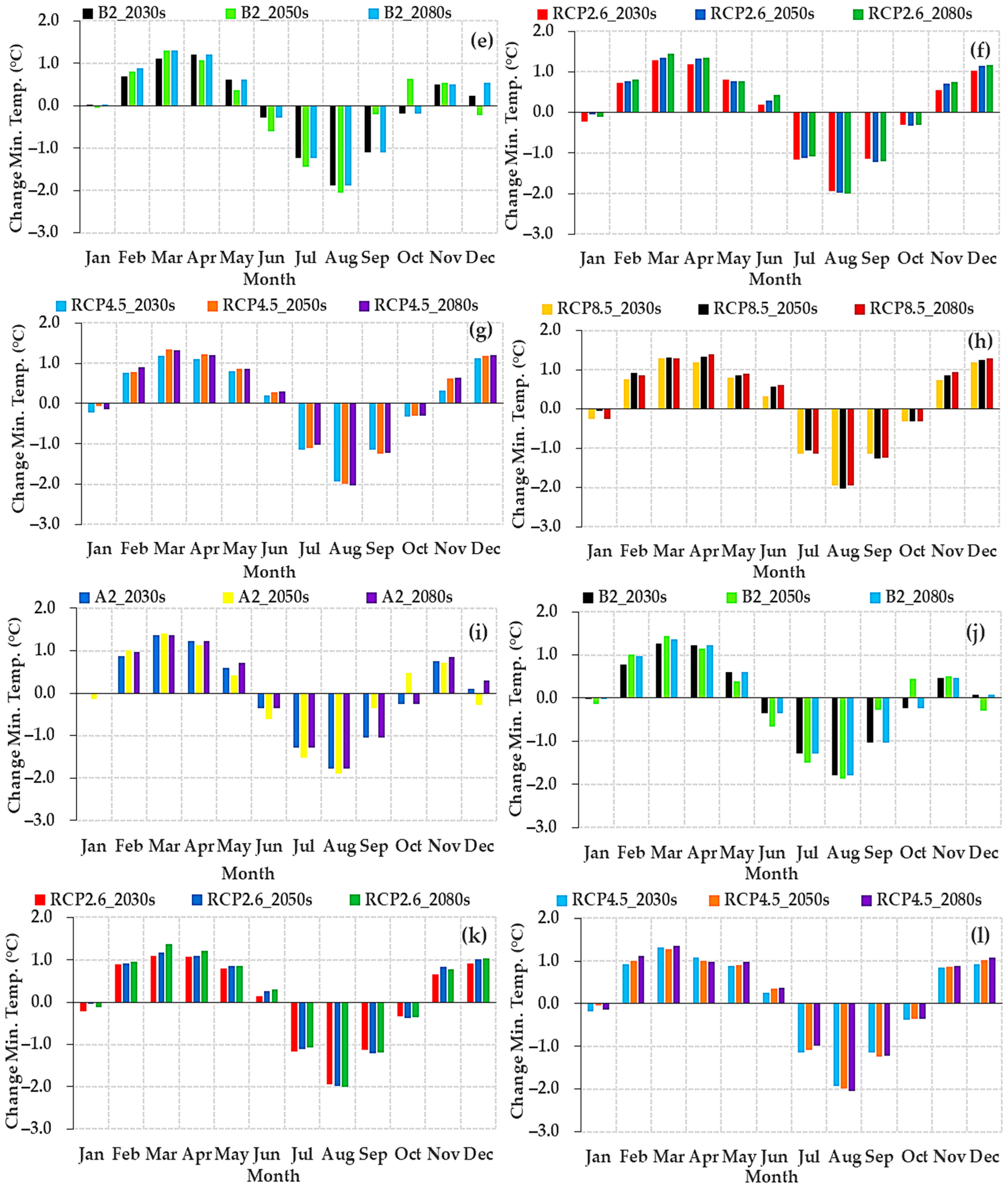
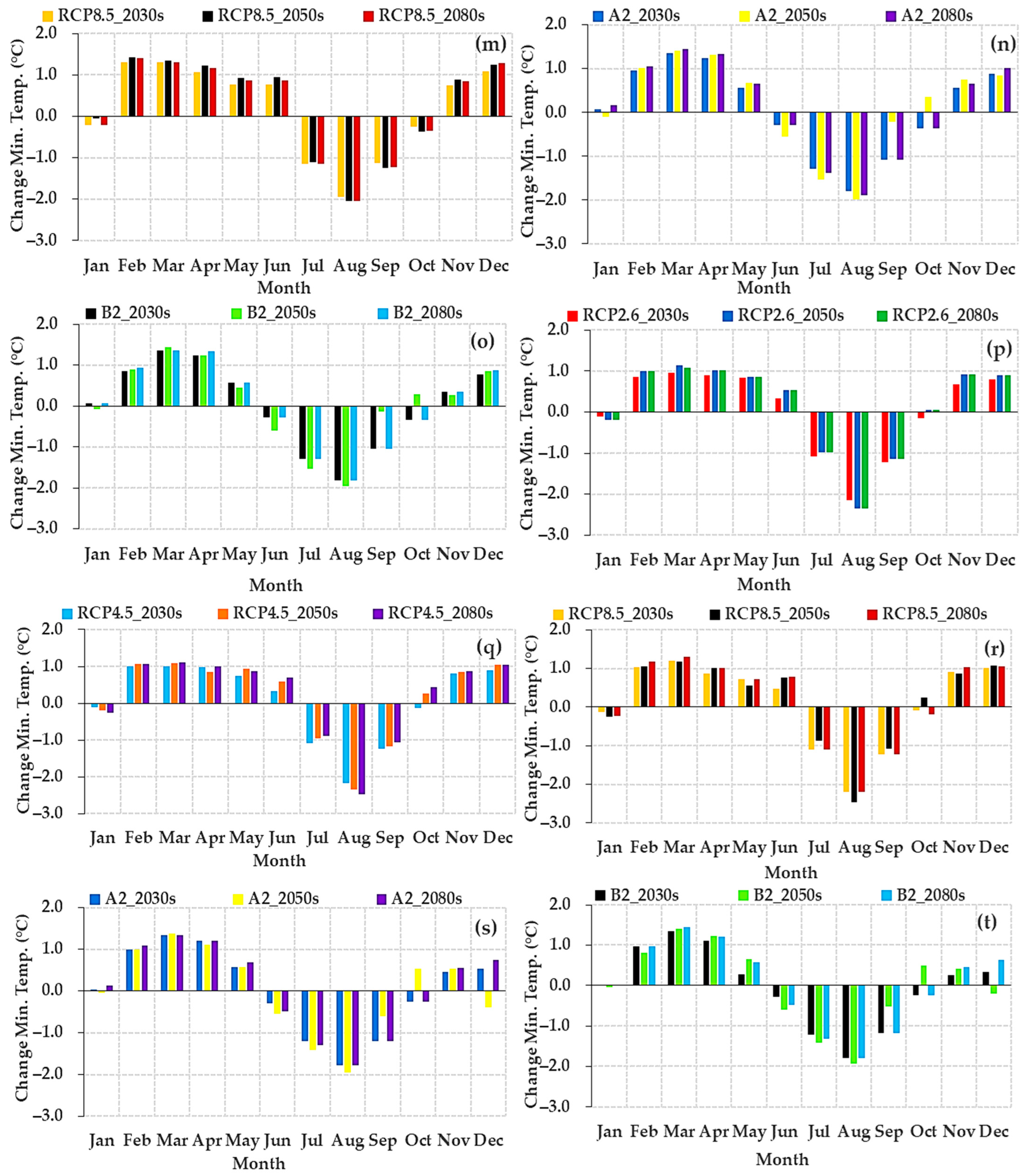
3.2.4. Change in Projected Future Monthly Minimum Temperature (T_min)

Figure 11a–t depict the projected future monthly change in T_min for the central region (Figure 11a–e), Greater Accra region (Figure 11f–j), Volta region (Figure 11k–o), and entire zone (Figure 11p–t) under the CanESM2 (RCP2.6, 4.5, and 8.5) and HadCM3 (A2 and B2) models for the 2030s, 2050s, and 2080s. The T_min follows a similar pattern to that of the T_max. In general, T_min is expected to increase in the 2030s, 2050s, and 2080s under both models for most months across the three regions and the entire zone (Figure 11a–t). T_min is projected to increase significantly more under the A2 scenario than under the B2 scenario for the HadCM3 model (Figure 11d,e,i,j,n,o,s,t). T_min is expected to increase significantly more under RCP8.5 than under the other two scenarios (Figure 11a–c, f–h, k–m, and p–r) across the three regions and the entire zone.

The results from Figure 11a–t show variation such as that of the T_max. Generally, T_min reveals a projected increase from the months of November to June, especially for the RCP scenarios. A similar pattern is observed under the A2 and B2 scenarios; however, the month of June decreases in that regard. That is, unlike the T_max, the T_min in the future will increase in the wet season, particularly in the month of June, as demonstrated by the RCP scenarios. While the T_min is expected to increase and decrease throughout the zone (Figure 11p–t), the projected rise and fall differ by region. T_min is expected to be the greatest (1.4 °C) and lowest (−2.1 °C) across the three regions, as well as the greatest (1.4 °C) and lowest (−2.3 °C) for the entire zone (Figure 11p–t). T_min is expected to vary the most (−2.3 and 1.4 °C) in Greater Accra and Volta and the least (−2.1 and 1.3 °C) in the central region. In general, the increase and decrease in T_min are considerably higher in the 2050s and 2080s across the three regions and the entire zone (Figure 11a–t). The overall comparison of the model results reveals a higher performance in the RCPs than in the A2 and B2 scenarios, like that of the T_max.

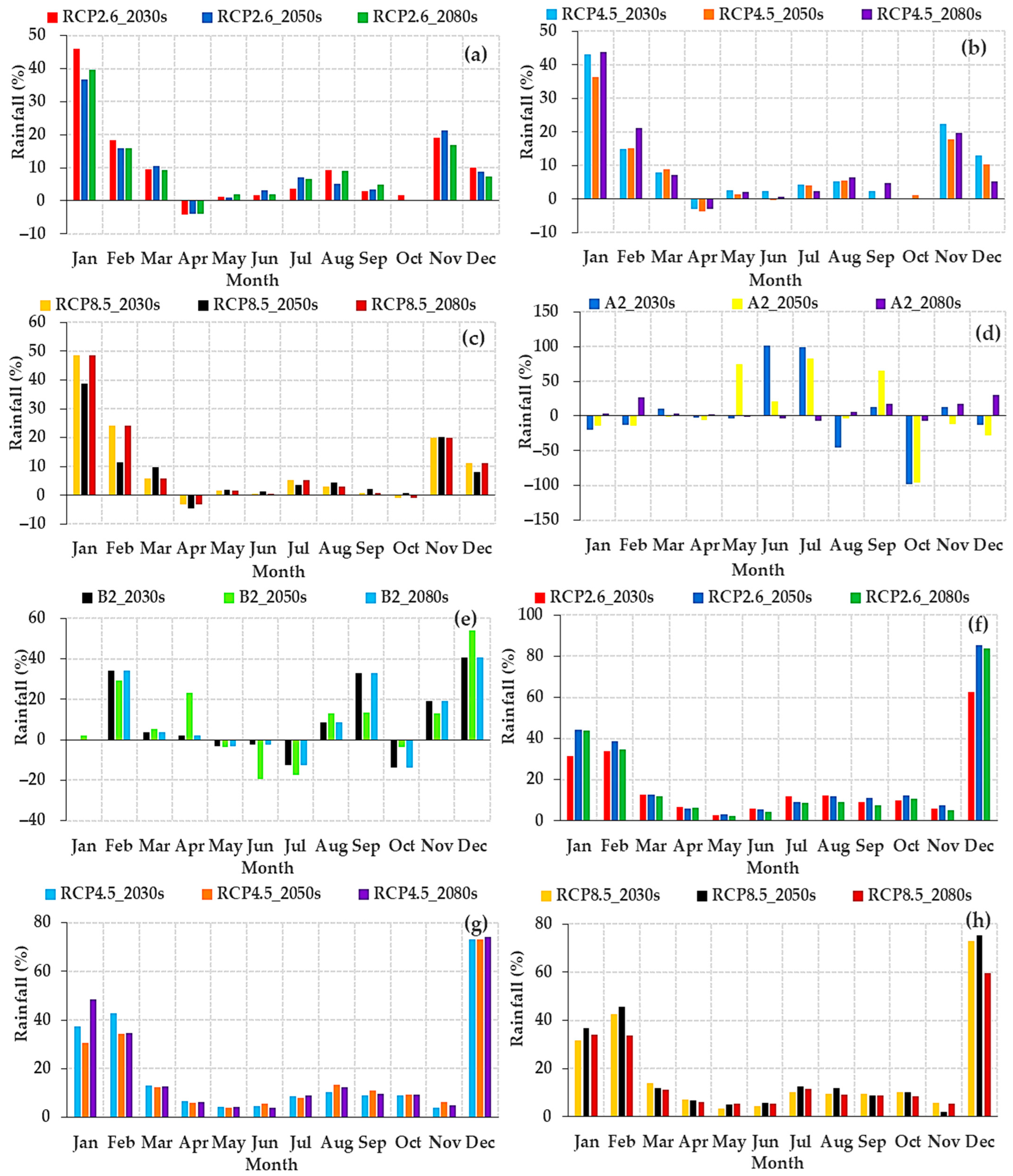
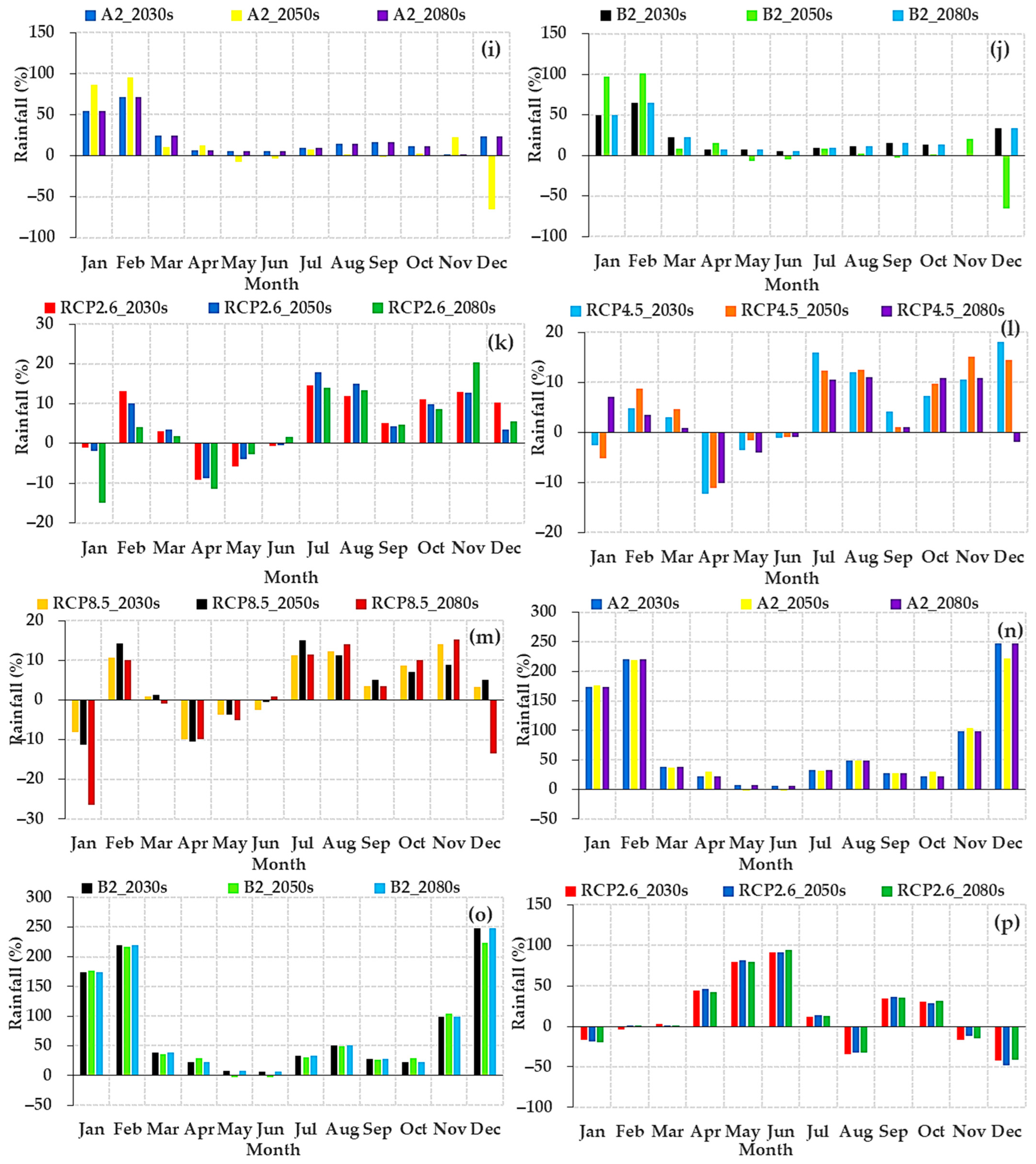
3.2.5. Change in Projected Future Monthly Rainfall

Figure 12a–t show the projected future monthly change in rainfall for the central region (Figure 12a–e), Greater Accra region (Figure 12f–j), Volta region (Figure 12k–o), and the entire zone (Figure 12p–t) for the 2030s, 2050s, and 2080s using the CanESM2 (RCP2.6, 4.5, and 8.5) and HadCM3 (A2 and B2 models). The overall results from Figure 12a–t indicate higher variations in rainfall in the 2030s, 2050s, and 2080s across the three regions and the entire zone under both models. In the central region, the A2 and B2 scenarios showed different projections for rainfall (Figure 12d–e). While rainfall is expected to increase and decrease for the wet season and minor and dry seasons, respectively, under the A2 scenarios (Figure 12d), the B2 scenario showed the opposite (Figure 12e). A dissimilar trend is observed for the Greater Accra region (Figure 12i,j). Here, rainfall is projected to increase under both the A2 and B2 scenarios (Figure 12i,j); however, the magnitude of change is greater for the dry season, especially from December to February. The projection for the Volta region (Figure 12n,o) follows a similar trend as the Greater Accra region. Here, rainfall is expected to increase in all months under both the A2 and B2 scenarios. Nevertheless, increases are expected to occur more in the future in the minor and dry seasons (September–March) compared to the wet season (April–July) (Figure 12n,o). The A2 and B2 scenarios for the entire zone tend to follow the zone’s normal double maxima rainfall season (Figure 12s–t). Here, rainfall is projected to increase in the wet, minor, and dry seasons except in the months of December (in the 2050s and 2080s) and August (in the 2030s, 2050s, and 2080s) under the A2 scenario. This is the same under the B2 scenario, just that here the decrease in December is expected to occur in the 2050s and in all the years in August. In comparing the A2 and B2 scenarios, it was observed that the scenario performance of the A2 was superior to the B2.

Under the RCP scenarios, rainfall is expected to increase in all months except April under all the RCP scenarios and in October in the 2080s under the RCP8.5 scenario for the central region (Figure 12a–c). Under the same scenarios, rainfall reveals projected increases in all months in the Greater Accra region, with the highest change occurring in the dry season (Figure 12f–h). In the Volta region, rainfall is projected to increase and decrease between the months (Figure 12k–m). For instance, under the RCP26, rainfall shows projected increases in all months except January, April, May, and June (in the 2030s and 2050s) (Figure 12k). The RCP4.5 and 8.5 follow a similar pattern to that of the RCP2.6. However, rainfall is expected to decrease in the month of December in the 2080s for both the RCP4.5 and 8.5 scenarios (Figure 12l–m). The results of rainfall for the entire zone under the RCP scenarios reveal a clear seasonal pattern (Figure 12p–r), as was observed under the A2 and B2 scenarios (Figure 12s–t). Here, rainfall shows a projected increase in the wet (April–July) and minor (September–October) seasons and a decrease in the dry (November–February), except for March. Nevertheless, the increase in March was weak.

Therefore, rainfall is expected to vary between −98.4 and 247.7% across the three regions and −29.0 and 148.0% for the entire zone under all scenarios. Among the three regions, rainfall is projected to decrease greatly in the central region (−98.4%) followed by the Greater Accra region (−65.8%) and least in the Volta region (−3.2%) whereas the Volta region is expected to receive more rainfall (247.7%), the central region (101.0%), and the Greater Accra region (100.6%). That is, in the future, monthly rainfall will increase greatly in the Volta and Greater Accra regions and decrease immensely in the central region. The overall model performance of the A2 and B2 scenarios surpasses that of the RCP scenarios for rainfall. For the A2 and B2 scenarios, rainfall is projected to vary greatly more under the A2 than in the B2 (Figure 12d,e,i,j,n,o,s,t). Under this scenario, rainfall is projected to increase by up to 247.7% in the 2030s and 2080s under the A2 and B2 scenarios, while under the RCP scenarios, rainfall is expected to increase by up to 96.0% in the 2050s and 2080s under the RCP8.5 (Figure 12a–c,f–h,k–m,p–r).

3.2.6. Projected Future Annual Change in Maximum (T_max) and Minimum (T_min) and Rainfall

Figure 13a–c show the projected future mean annual change in T_max (Figure 13a), T_min (Figure 13b), and rainfall (Figure 13c) for the 2030s, 2050s, and 2080s for the central, Greater Accra, and Volta regions and the entire zone under the CanESM2 (RCP2.6, 4.5, and 8.5) and the HadCM3 (A2 and B2) models. The results from Figure 13a–c reveal a considerable increase in T_max, T_min, and rainfall under both models. As shown in Figure 13a, T_max is expected to rise in all scenarios except the central region and the entire zone under RCP2.6. T_max is projected to increase greatly under the RCP8.5 scenario compared to the other two, while the A2 scenario surpasses the B2 (Figure 13a). Among the three regions, T_max reveals a greater increase in the Greater Accra region, especially under the RCP8.5 and the A2 scenarios, than the other two regions. The increase is also higher in the 2080s than in the 2030s and 2050s (Figure 13a). Notwithstanding the increase, the projected mean annual change is small. For example, the highest change in the mean annual T_max of 1.6 °C is expected to occur in the 2080s under the RCP8.5 scenario (Figure 13a). In general, the RCP scenarios outperformed the A2 and B2 scenarios.

The T_min follows a similar pattern to that of the T_max. Here, T_min is projected to increase in all years under all scenarios except in the 2030s under RCP4.5, A2, and B2 (Figure 13b). Under the RCP4.5 and A2, only the central region showed a decrease, while under the B2, T_min is expected to decrease in the central and Greater Accra regions and the entire zone (Figure 13b). The T_min shows a higher projected increase under all scenarios for the Greater Accra region than the other two. The T_min is expected to increase significantly in the 2050s under the RCP8.5 and A2 scenarios. In comparison to the T_max, the T_min shows greater annual change. Here, the highest mean annual change of T_min is 3.2 °C and is expected to occur in the 2050s under the RCP8.5 scenario (Figure 13b). Similar to the T_max, the overall results of the RCP scenarios surpassed the A2 and B2.

From Figure 13c, rainfall is projected to increase in all three regions and the entire zone under all scenarios. The minimum and maximum change in mean annual rainfall are expected to be between 0.8% (in the 2080s) and 79% (in the 2030s and 2080s) under the RCP8.5 and the A2 and B2 scenarios, respectively (Figure 13c). Among the three regions, the mean annual change in rainfall is expected to be highest in the Volta region, followed by the Greater Accra region, and least in the central region. Rainfall for the three regions and the entire zone show higher projections under the A2 and B2 scenarios than in the RCP scenarios. That is, for rainfall, the A2 and B2 scenarios in the HadCm3 model outperformed the RCPs in the CanESM2.

4. Discussion

In this study, we analyzed temperature (T_max and T_min) and rainfall extreme events and their trends over space and time and employed the SDSM tool to downscale future climate change scenarios based on the CanESM2 (RCP2.6, 4.5, and 8.5) and HadCM3 (A2 and B2) for the coastal Savannah agroecological zone of Ghana. Changes in temperature and rainfall from extreme events have significant implications for water supply, agriculture, livelihoods, and the health of the inhabitants in this region. The study identified more changepoints in T_min across the study locations. This finding is consistent with previous research studies conducted elsewhere on a national and global scale, such as [79,100,101,102,103,104].

The results revealed that the study region has warmed substantially in the past four decades. This result agrees with the earlier global research, such as [3,8,105,106]. The findings are also consistent with the previous research conducted at regional scales, such as [5,79,107,108]. According to the study’s findings, the SU25, TXn, and TN90p significantly increased for all locations, regions, and the entire zone, which is consistent with the previous findings such as [24,26,35,109,110,111,112,113,114]. Over the entire African continent, Iyakaremye et al. [115] state the increased number of warm nights in most parts of Africa, while Moberg et al. [116] report increased warming for the European territory. In furtherance to this, the results revealed a significant decrease in TN10p throughout the study locations and for the entire zone, which agrees with the earlier research studies, such as [25,26,87,117,118]. The IPCC [1], in its fifth assessment report, underlines a decrease in cool nights in many land regions, which is consistent with this study.

Spatially varied results were observed for the TXx, TNx, TNn, TX10p, TX90p, and the CSDI. Positive trends were observed only in the locations of Accra, Denu, and Tema for the TXx and Cape Coast, Denu, Elmina, Moree, Prampram, and the central and Volta regions for the TNx (see Table 5 and Figure 3). The TNn also significantly increased in the locations of Ada Foah, Anloga, Keta, and Saltpond. Again, the TX10p significantly decreases only in the locations of Accra, Cape Coast, Denu, Elmina, Moree, and Tema. This decrease was reflected in the three regions (the central, Greater Accra, and Volta), as well as for the entire zone. This conforms to the IPCC’s [1] assertions that cool days have decreased in many regions of the world. Moreover, the TX90p significantly increased only in the areas of Accra, Cape Coast, Denu, Elmina, Moree, Tema, and the Greater Accra region. The CSDI further showed both positive and negative trends. However, the positive trends, despite being significant, were weak. The CSDI, thus, decreased significantly in the locations of Denu, Elmina, and Moree, the three regions, and the entire zone. The variation in warming trends observed in this study is in line with the previous studies [79,119,120,121,122].

From the results, the DTR, an essential indicator of climate change [123,124], significantly decreased across the study region (−0.30 °C per decade). This finding is consistent with the earlier studies conducted in different regions, such as [26,125,126,127,128,129,130,131]. Barry et al. [26] state that the annual mean daily T_min has increased more than the annual mean daily T_max, which has led to a decreased DTR in the West African region, of which this study is no exception. It is worth noting that as far back as 1997, Easterling et al. [132] found a decreasing DTR trend in most parts of the world. The authors found factors such as increased cloudiness as key contributors to the decrease in DTR [132]. Nevertheless, Vose et al. [133] assert that after 1980, the increases in minimum and maximum temperatures have become more comparable, decreasing recent DTR trends. The recent increase in land-use changes through urbanization, population growth, and economic and industrial activities could be the cause of the decrease in the DTR in the zone. The coastal cities in Ghana, especially Accra (the capital), Tema, and Cape Coast, are known for their improved economic and industrial activities [73]. The incidence of urban heat island effects through urbanization and population growth has been found to decrease DTR [134,135].

The results revealed a significant decrease in RX1day, RX5day, SDII, and R10 only in the locations of Cape Coast, Elmina, Moree, and Saltpond, which was reflected in the general decrease for the central region, while the other locations were insignificant. This finding is consistent with previous research in other regions, such as [33,136,137,138]. In addition, the results of this study did not show any significant increase or decrease for R20, CWD, and PRCPTOT, which agrees with the earlier studies conducted elsewhere, such as [139,140]. Moreover, the CDD significantly decreased in the areas of Accra, Ada Foah, Anloga, Denu, Keta, Prampram, the Greater Accra and Volta regions, and the entire zone. This finding supports the earlier works conducted in other regions, such as [141,142]. The R95p and R99p, moreover, decreased significantly in the areas of Cape Coast, Elmina, Moree, and Saltpond, which reflected a significant decrease for the central region.

The results from the rainfall extreme indices revealed variations in the study region. For example, the decrease in RX1day, RX5day, SDII, and R10 was significant in most parts of the central region compared to the other two regions. A similar situation was observed for the R95p and R99p, while the CDD showed a significant decrease in the Greater Accra and Volta regions compared to the central region. This thus confirms the spatially variable nature of rainfall [24,29,143]. Other authors, including Abdullah et al. [79]; Vondou et al. [141]; and Santos et al. [142], reported highly variable extreme rainfall events in Bangladesh, Cameroon, and mainland Portugal, respectively. The results of the study revealed strong variations for the last four decades in the study regions, confirming the earlier work of Sanogo et al. [144] for the West African region and that of Nicholson [145] for the entire African continent.

The increase in global greenhouse gas emissions is believed to have made rainfall more variable over the West African region [146,147,148]. The decrease in rainfall is also attributed to land-ocean interactions and the related changes in sea surface temperature (SST) [148]. Notwithstanding, Dong and Sutton [148] believe that the increased levels of greenhouse gases in the atmosphere have a more substantial influence on the variable nature of rainfall in the West African region than the SST. Skinner et al. [149] contend that changes in SST caused by atmospheric radiative forcing are to blame for the decrease and variable nature of rainfall along most of the West African Guinea’s coast areas. According to Skinner et al. [149], changes in SST reduce the monsoon westerlies and the tropical easterly jet (TEJ), as well as low-level interconnection and rising air in the middle levels of the troposphere, causing decreasing rainfall over the region. Elsewhere, Abdullah et al. [79] and Shrestha et al. [107] reported decreased annual total rainfall for Bangladesh and India, respectively, in recent decades.

During the model performance assessment for calibration and validation for future climate change scenarios for the study region, it was observed that the performance in rainfall was low compared to the T_max and T_min, especially during validation of the model. This finding is consistent with the earlier studies, such as [44,45,56]. The poor performance could be attributed to the conditional modeling behavior of rainfall and the difficulty of achieving a perfect multiple regression in the SDSM. Wilby and Dawson [96] highlighted the fact that conditional models, such as the one applied to the case of rainfall, reveal an intermediate process between local weather and regional forcing. According to Siabi et al. [44], the dynamics of local weather, such as rainfall, are highly dependent on the number of wet and dry days, which in turn rely on regional-scale predictors such as atmospheric pressure and humidity, both of which are difficult for the SDSM to capture. Therefore, when compared to T_max and T_min, the process of downscaling rainfall is more challenging [150,151]. Gulacha and Mulungu [151] assert that the SDSM is possibly not the appropriate tool to downscale rainfall. The model performance results for T_max and T_min and rainfall in our study contradict the assertions of Gulacha and Mulungu [151]. In general, the present study achieved better calibration performance in all three climate variables analyzed (see Table 8) and is consistent with the earlier studies conducted elsewhere, such as [44,45,56,65,66].

The result from the performance of the two models showed that the CanESM2 (R² = 76–99%) outperformed the HadCM3 (R² = 58–99%) during calibration and validation. This finding is consistent with the previous future climate change projection studies, such as [45,59,60,152]. It is worth noting that several research studies, such as [44,153] have also reported better performance in the HadCM3 model compared to the CanESM2. The differences in model agreements, thus, reveal the uncertainty related to climate change assessment [60,154].

Generally, the results of monthly projections for both T_max and T_min revealed an increase for the 2030s, 2050s, and 2080s under both the CanESM2 (RCP2.6, 4.5, and 8.5) and HadCM3 (A2 and B2) models for three regions and the entire zone, amidst variations. The study zone’s three regions are expected to have the highest (1.6 °C) and lowest (−1.6 °C) T_max, while the entire zone is expected to have 1.5 °C and −1.6 °C. T_min will be the greatest (1.4 °C) and lowest (−2.1 °C) in each region, as well as the greatest (1.4 °C) and lowest (−2.3 °C) for the entire zone. Under the CanESM2 model, both T_max and T_min are projected to increase greatly under the RCP8.5 scenario, while that of the HadCM3 reveals a higher increase under the A2 scenarios. This finding is in line with the earlier studies, such as [44,45,56,59]. Under RCP8.5, the mean annual change in T_max and T_min is projected to be 1.6 °C (occurring in the 2080s) and 3.2 °C (occurring in the 2050s), respectively, which is similar to the change reported in an earlier study, such as [60].

The results from the projected monthly change in rainfall revealed variations among the three regions and the entire zone for the 2030s, 2050s, and 2080s under both models. Notwithstanding, the results obtained under both models showed more increases than decreases in rainfall. The decrease is more visible in the central region, while the Greater Accra and Volta regions showed an increase, thereby reflecting a general increase in rainfall in the future for the entire zone. For instance, rainfall is expected to vary between −98.4 and 247.7% across the three regions and −29.0 and 148.0% for the entire zone under all scenarios. This finding is in conformity with the earlier studies, such as [44,56]. The projected mean annual change in rainfall reveals an increase across the three regions and the entire zone. The mean annual rainfall in the zone is expected to vary between −0.8 and 79% under all scenarios. This finding agrees with studies such as [59,60].

The results of the study, therefore, have important implications for the coastal Savannah agroecological zone and the entire country. Although rainfall is projected to increase in the zone, it will be accompanied by greater variations. This situation could result in severe extreme events, including drought and floods in the zone. The incidence of both drought and flood events in the zone could have significant negative impacts on agricultural activities. For instance, a drought can lead to crop failures, losses, and the general drying of crops [155], while floods also have the tendency to damage seeds and seedlings and sweep away fertile soil [156]. The impacts of climate change on health are widely established in the scientific literature. For instance, Bosello et al. [157] assert that climate change will increase the range and abundance of vector-borne diseases, particularly malaria. There is also the possibility of a high incidence of diarrheal and intestinal diseases and cholera with the projected increase in rainfall. The projected increase in future rainfall in the zone will be beneficial for water resources, which will increase the annual river runoff.

5. Conclusions

Under a changing climate, the analysis of climate extreme indices and the projections for possible future climate change scenarios are relevant. The overall results of the study suggest that temperatures in the coastal Savannah agroecological zone of Ghana have increased and rainfall has become more variable over the last four decades, a feature that clearly supports the literature consensus on the variable nature of rainfall in the West African region. Both temperatures and rainfall are projected to increase in the future.

We noticed that most indices, such as SU25, TXn, and TN90p, significantly increased across the study locations, while others, such as TXx, TNx, TNn, TX10p, TX90p, and the CSDI, exhibited both increased and decreased trends, reflecting variations in the zone. The DTR, which is considered an essential indicator of climate change, significantly decreased across the study region. The majority of the extreme rainfall indices revealed a more significant decrease than an increase across the zone.

The general performance of the CanESM2 and HadCM3 models during calibration and validation was better, thereby supporting the encouragement for the usage of the SDSM technique in the literature for evaluating future possible climate change scenarios. The overall projection for both monthly and annual T_max and T_min showed an increase for the 2030s, 2050s, and 2080s under both the CanESM2 (RCP2.6, 4.5, and 8.5) and HadCM3 (A2 and B2) scenarios, agreeing with the consensus of a warming world and the need for increased mitigation and adaptation. Generally, both monthly and annual rainfall are projected to increase in the zone for the 2030s, 2050s, and 2080s under both models, amidst variations.

The findings of the study have several implications for agricultural activities, water resources, health, and the general livelihoods of the inhabitants in the study zone. The findings of this study could, therefore, be helpful for the development of appropriate adaptation plans to safeguard the livelihoods of people in the zone.

References

1. IPCC. Climate Change 2013: The Physical Science Basis. Contribution of Working Group I to the Fifth Assessment Report of the Intergovernmental Panel on Climate Change; Stocker, T.F., Qin, D., Plattner, G.-K., Tignor, M., Allen, S., Boschung, J., Nauels, A., Xia, Y., Bex, V., Midgley, P., Eds.; Cambridge University Press: Cambridge, UK; New York, NY, USA, 2013; p. 1535. [Google Scholar]
2. Folland, C.K.; Karl, T.R.; Jim Salinger, M. Observed climate variability and change. Weather 2002, 57, 269–278. [Google Scholar] [CrossRef]
3. Alexander, L.V.; Zhang, X.; Peterson, T.C.; Caesar, J.; Gleason, B.; Klein Tank, A.M.G.; Haylock, M.; Collins, D.; Trewin, B.; Rahimzadeh, F.; et al. Global observed changes in daily climate extremes of temperature and precipitation. J. Geophys. Res. Atmos. 2006, 111, 1–22. [Google Scholar] [CrossRef] [Green Version]
4. Maidment, R.I.; Allan, R.P.; Black, E. Recent observed and simulated changes in precipitation over Africa. Geophys. Res. Lett. 2015, 42, 1–10. [Google Scholar] [CrossRef]
5. Klein Tank, A.M.G.; Peterson, T.C.; Quadir, D.A.; Dorji, S.; Zou, X.; Tang, H.; Santhosh, K.; Joshi, U.R.; Jaswal, A.K.; Kolli, R.K.; et al. Changes in daily temperature and precipitation extremes in central and south Asia. J. Geophys. Res. Atmos. 2006, 111, 1–8. [Google Scholar] [CrossRef] [Green Version]
6. Worku, G.; Teferi, E.; Bantider, A.; Dile, Y.T. Observed changes in extremes of daily rainfall and temperature in Jemma sub-basin, upper blue Nile basin, Ethiopia. Theor. Appl. Climatol. 2019, 135, 839–854. [Google Scholar] [CrossRef]
7. da Silva, P.E.; Santos e Silva, C.M.; Spyrides, M.H.C.; Andrade, L.D.M.B. Precipitation and air temperature extremes in the Amazon and northeast Brazil. Int. J. Climatol. 2019, 39, 579–595. [Google Scholar] [CrossRef]
8. Easterling, D.R.; Evans, J.L.; Groisman, P.Y.; Karl, T.R.; Kunkel, K.E.; Ambenje, P. Observed variability and trends in extreme climate events: A brief review. Bull. Am. Meteorol. Soc. 2000, 81, 417–425. [Google Scholar] [CrossRef]
9. Sharma, D.; Babel, M.S. Trends in extreme rainfall and temperature indices in the western Thailand. Int. J. Climatol. 2014, 34, 2393–2407. [Google Scholar] [CrossRef]
10. Peterson, T.C.; Manton, M.J. Monitoring changes in climate extremes: A tale of international collaboration. Bull. Am. Meteorol. Soc. 2008, 89, 1266–1271. [Google Scholar] [CrossRef]
11. Tierney, J.E.; Smerdon, J.E.; Anchukaitis, K.J.; Seager, R. Multidecadal variability in East African hydroclimate controlled by the Indian Ocean. Nature 2013, 493, 389–392. [Google Scholar] [CrossRef] [Green Version]
12. IPCC. Managing The Risks of Extreme Events and Disasters to Advance Climate Change Adaptation; A special report of working groups I and II of the intergovernmental panel on climate change (IPCC); Field, C.B., Barros, V., Stocker, T., Qin, D., Dokken, D., Ebi, K., Mastrandrea, M., Mach, K., Plattner, G.-K., Allen, S., et al., Eds.; Cambridge University Press: Cambridge, UK; New York, NY, USA, 2012; pp. 555–564. [Google Scholar]
13. Frich, P.; Alexander, L.V.; Della-Marta, P.; Gleason, B.; Haylock, M.; Tank Klein, A.M.G.; Peterson, T. Observed coherent changes in climatic extremes during the second half of the twentieth century. Clim. Res. 2002, 19, 193–212. [Google Scholar] [CrossRef] [Green Version]
14. Manton, M.; Della-Marta, P.; Haylock, M.; Hennessy, K.; Nicholls, N.; Chambers, L.; Collins, D.; Daw, G.; Finet, A.; Gunawan, D.; et al. Trends in extreme daily rainfall and temperature in southeast Asia and the south Pacific: 1961–1998. Int. J. Climatol. 2001, 21, 269–284. [Google Scholar] [CrossRef]
15. Peterson, T.C.; Taylor, M.A.; Demeritte, R.; Duncombe, D.L.; Burton, S.; Thompson, F.; Porter, A.; Mercedes, M.; Villegas, E.; Fils, R.S.; et al. Recent changes in climate extremes in the Caribbean region. J. Geophys. Res. Atmos. 2002, 107, 1–9. [Google Scholar] [CrossRef] [Green Version]
16. Karl, T.R.; Knight, R.W.; Easterling, D.R.; Quayle, R.G. Indices of climate change for the United States. Bull. Am. Meteorol. Soc. 1996, 77, 279–292. [Google Scholar] [CrossRef]
17. Vincent, L.A.; Mekis, É. Changes in daily and extreme temperature and precipitation indices for Canada over the twentieth century. Atmos.Ocean 2006, 44, 177–193. [Google Scholar] [CrossRef] [Green Version]
18. Klein Tank, A.M.G.; Können, G.P. Trends in indices of daily temperature and precipitation extremes in Europe, 1946–1999. J. Clim. 2003, 16, 3665–3680. [Google Scholar] [CrossRef]
19. You, Q.; Kang, S.; Aguilar, E.; Yan, Y. Changes in daily climate extremes in the eastern and central Tibetan plateau during 1961–2005. J. Geophys. Res. Atmos. 2008, 113, 1–17. [Google Scholar] [CrossRef] [Green Version]
20. Haylock, M.R.; Peterson, T.C.; Alves, L.M.; Ambrizzi, T.; Anunciação, Y.M.T.; Baez, J.; Barros, V.R.; Berlato, M.A.; Bidegain, M.; Coronel, G.; et al. Trends in total and extreme South American rainfall in 1960–2000 and links with sea surface temperature. J. Clim. 2006, 19, 1490–1512. [Google Scholar] [CrossRef]
21. Vincent, L.A.; Peterson, T.C.; Barros, V.R.; Marino, M.B.; Rusticucci, M.; Carrasco, G.; Ramirez, E.; Alves, L.M.; Ambrizzi, T.; Berlato, M.A.; et al. Observed trends in indices of daily temperature extremes in South America 1960–2000. J. Clim. 2005, 18, 5011–5023. [Google Scholar] [CrossRef]
22. Alexander, L.V.; Hope, P.; Collins, D.; Trewin, B.; Lynch, A.; Nicholls, N. Trends in Australia’s climate means and extremes: A global context. Aust. Meteorol. Mag. 2007, 56, 1–18. [Google Scholar]
23. Guerreiro, S.B.; Fowler, H.J.; Barbero, R.; Westra, S.; Lenderink, G.; Blenkinsop, S.; Lewis, E.; Li, X.F. Detection of continental-scale intensification of hourly rainfall extremes. Nat. Clim. Chang. 2018, 8, 803–807. [Google Scholar] [CrossRef] [Green Version]
24. New, M.; Hewitson, B.; Stephenson, D.B.; Tsiga, A.; Kruger, A.; Manhique, A.; Gomez, B.; Coelho, C.A.S.; Masisi, D.N.; Kululanga, E.; et al. Evidence of trends in daily climate extremes over Southern and West Africa. J. Geophys. Res. Atmos. 2006, 111, 1–11. [Google Scholar] [CrossRef]
25. Omondi, P.A.; Awange, J.L.; Forootan, E.; Ogallo, L.A.; Barakiza, R.; Girmaw, G.B.; Fesseha, I.; Kululetera, V.; Kilembe, C.; Mbati, M.M.; et al. Changes in temperature and precipitation extremes over the Greater Horn of Africa region from 1961 to 2010. Int. J. Climatol. 2014, 34, 1262–1277. [Google Scholar] [CrossRef]
26. Barry, A.A.; Caesar, J.; Klein Tank, A.M.G.; Aguilar, E.; McSweeney, C.; Cyrille, A.M.; Nikiema, M.P.; Narcisse, K.B.; Sima, F.; Stafford, G.; et al. West Africa climate extremes and climate change indices. Int. J. Climatol. 2018, 38, e921–e938. [Google Scholar] [CrossRef]
27. Sylla, M.B.; Giorgi, F.; Coppola, E.; Mariotti, L. Uncertainties in daily rainfall over Africa: Assessment of gridded observation products and evaluation of a regional climate model simulation. Int. J. Climatol. 2013, 33, 1805–1817. [Google Scholar] [CrossRef]
28. Ben Mohamed, A. Climate change risks in Sahelian Africa. Reg. Environ. Chang. 2011, 11 (Suppl. S1), 109–117. [Google Scholar] [CrossRef]
29. Panthou, G.; Vischel, T.; Lebel, T. Recent trends in the regime of extreme rainfall in the Central Sahel. Int. J. Climatol. 2014, 34, 3998–4006. [Google Scholar] [CrossRef]
30. Monerie, P.-A.; Fontaine, B.; Roucou, P. Expected future changes in the African monsoon between 2030 and 2070 using some CMIP3 and CMIP5 models under a medium-low RCP scenario. J. Geophys. Res. 2012, 117, D16111. [Google Scholar] [CrossRef] [Green Version]
31. De Longueville, F.; Hountondji, Y.C.; Kindo, I.; Gemenne, F.; Ozer, P. Long-term analysis of rainfall and temperature data in Burkina Faso (1950–2013). Int. J. Climatol. 2016, 36, 4393–4405. [Google Scholar] [CrossRef]
32. Hountondji, Y.-C.; De Longueville, F.; Ozer, P. Trends in extreme rainfall events in Benin (West Africa), 1960–2000. In Proceedings of the 1st International Conference on Energy, Environment and Climate Change, Ho Chi Minh City, Vietnam, 26–27 August 2011. [Google Scholar]
33. Obada, E.; Alamou, E.A.; Biao, E.I.; Zandagba, E.B.J. Interannual variability and trends of extreme rainfall indices over Benin. Climate 2021, 9, 160. [Google Scholar] [CrossRef]
34. Mouhamed, L.; Traore, S.B.; Alhassane, A.; Sarr, B. Evolution of some observed climate extremes in the West African Sahel. Weather Clim. Extrem. 2013, 1, 19–25. [Google Scholar] [CrossRef] [Green Version]
35. Larbi, I.; Hountondji, F.C.C.; Annor, T.; Agyare, W.A.; Gathenya, J.M.; Amuzu, J. Spatio-temporal trend analysis of rainfall and temperature extremes in the Vea Catchment, Ghana. Climate 2018, 6, 87. [Google Scholar] [CrossRef] [Green Version]
36. Atiah, W.A.; Muthoni, F.K.; Kotu, B.; Kizito, F.; Amekudzi, L.K. Trends of rainfall onset, cessation, and length of growing season in northern Ghana: Comparing the rain gauge, satellite, and farmer’s perceptions. Atmosphere 2021, 12, 1674. [Google Scholar] [CrossRef]
37. Braimah, M.; Asante, V.A.; Ahiataku, M.A.; Ansah, S.O.; Otu-Larbi, F.; Yahaya, B.; Ayabilah, J.B.; Nkrumah, F. Variability of the minor season rainfall over southern Ghana (1981–2018). Adv. Meteorol. 2022, 2022, 1861130. [Google Scholar] [CrossRef]
38. Cooper, P.J.M.; Dimes, J.; Rao, K.P.C.; Shapiro, B.; Shiferaw, B.; Twomlow, S. Coping better with current climatic variability in the rain-fed farming systems of Sub-Saharan Africa: An essential first step in adapting to future climate change? Agric. Ecosyst. Environ. 2008, 126, 24–35. [Google Scholar] [CrossRef] [Green Version]
39. Sultan, B.; Gaetani, M. Agriculture in West Africa in the twenty-first century: Climate change and impacts scenarios, and potential for adaptation. Front. Plant Sci. 2016, 7, 1–20. [Google Scholar] [CrossRef] [Green Version]
40. Antwi-Agyei, P.; Fraser, E.D.G.; Dougill, A.J.; Stringer, L.C.; Simelton, E. Mapping the vulnerability of crop production to drought in Ghana using rainfall, yield and socioeconomic data. Appl. Geogr. 2012, 32, 324–334. [Google Scholar] [CrossRef]
41. Owusu, K.; Waylen, P.R. The changing rainy season climatology of mid-Ghana. Theor. Appl. Climatol. 2013, 112, 419–430. [Google Scholar] [CrossRef]
42. Zhang, X.; Alexander, L.; Hegerl, G.C.; Jones, P.; Tank, A.K.; Peterson, T.C.; Trewin, B.; Zwiers, F.W. Indices for monitoring changes in extremes based on daily temperature and precipitation data. Wiley Interdiscip. Rev. Clim. Chang. 2011, 2, 851–870. [Google Scholar] [CrossRef]
43. IPCC. Summary for Policymakers. In Global Warming of 1.5 °C. An IPCC Special Report on the Impacts of Global Warming of 1.5 °C above Pre-Industrial Levels and Related Global Greenhouse Gas Emission Pathways, in the Context of Strengthening the Global Response to the Threat of Climate Change, Sustainable Development, and Efforts to Eradicate Poverty; Masson-Delmotte, V., Zhai, P., Pörtner, H.-O., Roberts, D., Skea, J., Shukla, P., Pirani, A., Moufouma-Okia, W., Péan, C., Pidcock, R., et al., Eds.; Cambridge University Press: Cambridge, UK; New York, NY, USA, 2018; pp. 3–24. [Google Scholar] [CrossRef]
44. Siabi, E.K.; Kabobah, A.T.; Akpoti, K.; Anornu, G.K.; Amo-boateng, M.; Nyantakyi, E.K. Statistical downscaling of global circulation models to assess future climate changes in the Black Volta basin of Ghana. Environ. Challenges 2021, 5, 100299. [Google Scholar] [CrossRef]
45. Phuong, D.N.D.; Duong, T.Q.; Liem, N.D.; Tram, V.N.Q.; Cuong, D.K.; Loi, N.K. Projections of future climate change in the Vu Gia Thu Bon River Basin, Vietnam by using statistical downscaling model (SDSM). Water 2020, 12, 755. [Google Scholar] [CrossRef] [Green Version]
46. Arnell, N.W.; Lowe, J.A.; Bernie, D.; Nicholls, R.J.; Brown, S.; Challinor, A.J.; Osborn, T.J. The global and regional impacts of climate change under representative concentration pathway forcings and shared socioeconomic pathway socioeconomic scenarios. Environ. Res. Lett. 2019, 14, 084046. [Google Scholar] [CrossRef]
47. James, R.; Washington, R.; Rowell, D.P. African climate change uncertainty in perturbed physics ensembles: Implications of global warming to 4 °C and beyond. J. Clim. 2014, 27, 4677–4692. [Google Scholar] [CrossRef]
48. Diedhiou, A.; Bichet, A.; Wartenburger, R.; Seneviratne, S.I.; Rowell, D.P. Changes in climate extremes over West and Central Africa at 1.5 °C and 2 °C global warming. Environ. Res. Lett. 2018, 13, 065020. [Google Scholar] [CrossRef]
49. Endris, H.S.; Omondi, P.; Jain, S.; Lennard, C.; Hewitson, B.; Chang’a, L.; Awange, J.L.; Dosio, A.; Ketiem, P.; Nikulin, G.; et al. Assessment of the performance of CORDEX regional climate models in simulating East African rainfall. J. Clim. 2013, 26, 8453–8475. [Google Scholar] [CrossRef]
50. Shongwe, M.E.; van Oldenborgh, G.J.; van den Hurk, B.J.J.M.; de Boer, B.; Coelho, C.A.S.; van Aalst, M.K. Projected changes in mean and extreme precipitation in Africa under global warming. Part I: Southern Africa. J. Clim. 2009, 22, 3819–3837. [Google Scholar] [CrossRef]
51. Wilby, R.L.; Wigley, T.M.L. Downscaling general circulation model output: A review of methods and limitations. Prog. Phys. Geogr. Earth Environ. 1997, 21, 530–548. [Google Scholar] [CrossRef] [Green Version]
52. Benestad, R.E. Empirical-statistical downscaling in climate modeling. EOS Trans. Am. Geophys. Union 2004, 85, 417–422. [Google Scholar] [CrossRef]
53. Wilby, R.L.; Dawson, C.W. Using SDSM Version 3.1—A Decision Support Tool for the Assessment of Regional Climate Change Impacts. User Man. 2004, 8, 1–7. Available online: https://unfccc.int/resource/cd_roms/na1/v_and_a/Resoursce_materials/Climate/SDSM/SDSM.Manual.pdf (accessed on 28 August 2022).
54. Semenov, M.A.; Barrow, E.M. A Stochastic Weather Generator for Use in Climate Impact Studies; User Manual: Hertfordshire, UK, 2002; pp. 1–27. Available online: http://resources.rothamsted.ac.uk/sites/default/files/groups/mas-models/download/LARS-WG-Manual.pdf (accessed on 28 August 2022).
55. Akbari, H.; Rakhshandehroo, G.R.; Afrooz, A.H.; Pourtouiserkani, A. Climate change impact on intensity-duration-frequency curves in Chenar-Rahdar river basin. Watershed Manag. 2015, 5, 48–61. [Google Scholar] [CrossRef]
56. Birara, H.; Mishra, R.P.P.S.K. Projections of future rainfall and temperature using statistical downscaling techniques in Tana Basin, Ethiopia. Sustain. Water Resour. Manag. 2020, 6, 1–17. [Google Scholar] [CrossRef]
57. Daksiya, V.; Mandapaka, P.; Lo, E.Y.M. A comparative frequency analysis of maximum daily rainfall for a SE Asian region under current and future climate conditions. Adv. Meteorol. 2017, 2017, 2620798. [Google Scholar] [CrossRef] [Green Version]
58. Gebrechorkos, S.H.; Hülsmann, S.; Bernhofer, C. Statistically downscaled climate dataset for East Africa. Sci. Data 2019, 6, 31. [Google Scholar] [CrossRef] [PubMed] [Green Version]
59. Iwadra, M.; Odirile, P.T.; Parida, B.P.; Moalafhi, D.B. Evaluation of future climate using SDSM and secondary data (TRMM and NCEP) for poorly gauged catchments of Uganda: The case of Aswa catchment. Theor. Appl. Climatol. 2019, 137, 2029–2048. [Google Scholar] [CrossRef]
60. Fenta Mekonnen, D.; Disse, M. Analyzing the future climate change of upper blue Nile River basin using statistical downscaling techniques. Hydrol. Earth Syst. Sci. 2018, 22, 2391–2408. [Google Scholar] [CrossRef] [Green Version]
61. Vallam, P.; Qin, X.S. Projecting future precipitation and temperature at sites with diverse climate through multiple statistical downscaling schemes. Theor. Appl. Climatol. 2018, 134, 669–688. [Google Scholar] [CrossRef]
62. Campozano, L.; Tenelanda, D.; Sanchez, E.; Samaniego, E.; Feyen, J. Comparison of statistical downscaling methods for monthly total precipitation: Case study for the Paute River basin in southern Ecuador. Adv. Meteorol. 2016, 2016, 6526341. [Google Scholar] [CrossRef] [Green Version]
63. Etemadi, H.; Samadi, S.; Sharifikia, M. Uncertainty analysis of statistical downscaling models using general circulation model over an international wetland. Clim. Dyn. 2014, 42, 2899–2920. [Google Scholar] [CrossRef]
64. Hashmi, M.Z.; Shamseldin, A.Y.; Melville, B.W. Comparison of SDSM and LARS-WG for simulation and downscaling of extreme precipitation events in a watershed. Stoch. Environ. Res. Risk Assess. 2011, 25, 475–484. [Google Scholar] [CrossRef]
65. Liu, Z.; Xu, Z.; Charles, S.P.; Fu, G.; Liu, L. Evaluation of two statistical downscaling models for daily precipitation over an arid basin in China. Int. J. Climatol. 2011, 31, 2006–2020. [Google Scholar] [CrossRef]
66. Najafi, R.; Hessami Kermani, M. Uncertainty modeling of statistical downscaling to assess climate change impacts on temperature and precipitation. Water Resour. Manag. 2017, 31, 1843–1858. [Google Scholar] [CrossRef]
67. Khan, M.S.; Coulibaly, P.; Dibike, Y. Uncertainty analysis of statistical downscaling methods. J. Hydrol. 2006, 319, 357–382. [Google Scholar] [CrossRef]
68. Khan, M.S.; Coulibaly, P.; Dibike, Y. Uncertainty analysis of statistical downscaling methods using Canadian Global Climate Model predictors. Hydrol. Process. 2006, 20, 3085–3104. [Google Scholar] [CrossRef]
69. Bessah, E.; Boakye, E.A.; Agodzo, S.K.; Nyadzi, E.; Larbi, I.; Awotwi, A. Increased seasonal rainfall in the twenty-first century over Ghana and its potential implications for agriculture productivity. Environ. Dev. Sustain. 2021, 23, 12342–12365. [Google Scholar] [CrossRef]
70. Bessah, E.; Raji, A.O.; Taiwo, O.J.; Agodzo, S.K.; Ololade, O.O. Variable resolution modeling of near future mean temperature changes in the dry sub-humid region of Ghana. Model. Earth Syst. Environ. 2018, 4, 919–933. [Google Scholar] [CrossRef]
71. Larbi, I.; Hountondji, F.C.C.; Dotse, S.; Mama, D.; Nyamekye, C.; Adeyeri, O.E.; Djan, H.; Rock, P.; Odoom, E.; Mensah, Y. Local climate change projections and impact on the surface hydrology in the Vea Catchment, West Africa. Hydrol. Res. 2021, 52, 1200–1215. [Google Scholar] [CrossRef]
72. Addi, M.; Asare, K.; Fosuhene, S.K.; Ansah-Narh, T.; Aidoo, K.; Botchway, C.G. Impact of large-scale climate indices on meteorological drought of coastal Ghana. Adv. Meteorol. 2021, 2021, 8899645. [Google Scholar] [CrossRef]
73. Ghana Statistical Service. 2010 Population and Housing Census. National Analytical Report. 2013. Available online: https://statsghana.gov.gh/gssmain/fileUpload/pressrelease/2010_PHC_National_Analytical_Report.pdf (accessed on 27 August 2022).
74. Dickson, K.B.; Benneh, G. A New Geography of Ghana; Revised edition; Longman Group Ltd.: Essex, UK, 1995; pp. 17–40. [Google Scholar]
75. Wilby, R.L.; Dawson, C.W.; Murphy, C.; O’Connor, P.; Hawkins, E. The Statistical downscaling model-decision centric (SDSM-DC): Conceptual basis and applications. Clim. Res. 2014, 61, 259–276. [Google Scholar] [CrossRef] [Green Version]
76. Graham, J.W. Missing data analysis: Making it work in the real world. Annu. Rev. Psychol. 2009, 60, 549–576. [Google Scholar] [CrossRef] [Green Version]
77. Schafer, J.L.; Graham, J.W. Missing data: Our view of the state of the art. Psychol. Methods 2002, 7, 147–177. [Google Scholar] [CrossRef]
78. Zhang, Z. Multiple imputation with multivariate imputation by chained equation (MICE) package. Ann. Transl. Med. 2016, 4, 30. [Google Scholar] [CrossRef] [PubMed]
79. Abdullah, A.Y.M.; Bhuian, M.H.; Kiselev, G.; Dewan, A.; Hassan, Q.K.; Rafiuddin, M. Extreme temperature and rainfall events in Bangladesh: A comparison between coastal and inland areas. Int. J. Climatol. 2022, 42, 3253–3273. [Google Scholar] [CrossRef]
80. Azur, M.J.; Stuart, E.A.; Frangakis, C.; Leaf, P.J. Multiple imputation by chained equations: What is it and how does it work? Int. J. Methods Psychiatr. Res. 2011, 20, 40–49. [Google Scholar] [CrossRef] [PubMed]
81. Zhang, X.; Yang, F. RClimDex (1.0) User Manual. Climate Research Branch Environment Canada. 2004. Available online: http://www.acmad.net/rcc/procedure/RClimDexUserManual.pdf (accessed on 27 August 2022).
82. Wang, X.; Feng, Y. RHTestV4 User Manual; Climate Research Division, Atmospheric Science and Technology Directorate, Science and Technology Branch, Environment Canada: Toronto, ON, Canada, 2013; Available online: http://cccma.seos.uvic.ca/ETCCDMI/RHTest/RHTestUserManual.doc (accessed on 27 August 2022).
83. Wang, X.L. Accounting for autocorrelation in detecting mean shifts in climate data series using the penalized maximal t or F test. J. Appl. Meteorol. Climatol. 2008, 47, 2423–2444. [Google Scholar] [CrossRef]
84. Wang, X.L. Penalized maximal F test for detecting undocumented mean shift without trend change. J. Atmos. Ocean. Technol. 2008, 25, 368–384. [Google Scholar] [CrossRef]
85. Wang, X.L.; Feng, Y. RHtests_dlyPrcp User Manual; Climate Research Division, Atmospheric Science and Technology Directorate, Science and Technology Branch, Environment Canada: Toronto, ON, Canada, 2013; Available online: http://etccdi.pacificclimate.org/software.shtml. (accessed on 27 August 2022).
86. Ruml, M.; Gregorić, E.; Vujadinović, M.; Radovanović, S.; Matović, G.; Vuković, A.; Počuča, V.; Stojičić, D. Observed changes of temperature extremes in Serbia over the period 1961−2010. Atmos. Res. 2017, 183, 26–41. [Google Scholar] [CrossRef]
87. Sein, K.K.; Chidthaisong, A.; Oo, K.L. Observed trends and changes in temperature and precipitation extreme indices over Myanmar. Atmosphere 2018, 9, 477. [Google Scholar] [CrossRef] [Green Version]
88. Wang, X.L.; Chen, H.; Wu, Y.; Feng, Y.; Pu, Q. New techniques for the detection and adjustment of shifts in daily precipitation data series. J. Appl. Meteorol. Climatol. 2010, 49, 2416–2436. [Google Scholar] [CrossRef]
89. Mann, H.B. Nonparametric tests against trend. Econometrica 1945, 13, 245–259. [Google Scholar] [CrossRef]
90. Kendall, M.G. Rank Correlation Methods; Griffin: London, UK, 1975. [Google Scholar]
91. Sen, P.K. Estimates of the regression coefficient based on Kendall’s tau. J. Am. Stat. Assoc. 1968, 63, 1379–1389. [Google Scholar] [CrossRef]
92. da Silva, R.M.; Santos, C.A.G.; Moreira, M.; Corte-Real, J.; Silva, V.C.L.; Medeiros, I.C. Rainfall and river flow trends using Mann–Kendall and Sen’s slope estimator statistical tests in the Cobres River basin. Nat. Hazards 2015, 77, 1205–1221. [Google Scholar] [CrossRef]
93. Derrick, B.; Toher, D.; White, P. Why Welch’s test is Type I error robust. Quant. Methods Psychol. 2016, 12, 30–38. [Google Scholar] [CrossRef]
94. Wilby, R.L.; Dawson, C.W.; Barrow, E.M. SDSM—a decision support tool for the assessment of regional climate change impacts. Environ. Model. Softw. 2002, 17, 145–157. [Google Scholar] [CrossRef]
95. Wilby, R.L.; Charles, S.; Mearns, L.O.; Whetton, P.; Zorito, E.; Timbal, B. Guidelines for use of climate scenarios developed from statistical downscaling methods. IPCC Task Group on Scenarios for Climate Impact Assessment (TGCIA). 2004. Available online: http://www.ipccdata.org/guidelines/dgmno2v1092004.pd (accessed on 27 August 2022).
96. Wilby, R.L.; Dawson, C.W. SDSM 4.2-A Decision Support Tool for the Assessment of Regional Climate Change Impacts; User Manual; Lancaster University: Lancaster, UK; Environment Agency England: Wales, UK, 2007; Volume 94, pp. 1–94. [Google Scholar]
97. Wilby, R.L.; Dawson, C.W. The statistical downscaling model: Insights from one decade of application. Int. J. Climatol. 2013, 33, 1707–1719. [Google Scholar] [CrossRef]
98. Mahmood, R.; Babel, M.S. Future changes in extreme temperature events using the statistical downscaling model (SDSM) in the trans-boundary region of the Jhelum river basin. Weather. Clim. Extrem. 2014, 5, 56–66. [Google Scholar] [CrossRef] [Green Version]
99. Fan, X.; Jiang, L.; Gou, J. Statistical downscaling and projection of future temperatures across the Loess Plateau, China. Weather Clim. Extrem. 2021, 32, 100328. [Google Scholar] [CrossRef]
100. Cao, L.; Zhu, Y.; Tang, G.; Yuan, F.; Yan, Z. Climatic warming in China according to a homogenized data set from 2419 stations. Int. J. Climatol. 2016, 36, 4384–4392. [Google Scholar] [CrossRef] [Green Version]
101. Li, Q.; Dong, W. Detection and adjustment of undocumented discontinuities in Chinese temperature series using a composite approach. Adv. Atmos. Sci. 2009, 26, 143–153. [Google Scholar] [CrossRef]
102. Jaiswal, R.K.; Lohani, A.K.; Tiwari, H.L. Statistical analysis for change detection and trend assessment in climatological parameters. Environ. Process. 2015, 2, 729–749. [Google Scholar] [CrossRef] [Green Version]
103. Sarangi, C.; Qian, Y.; Li, J.; Leung, L.R.; Chakraborty, T.C.; Liu, Y. Urbanization amplifies nighttime heat stress on warmer days over the US. Geophys. Res. Lett. 2021, 48, 1–12. [Google Scholar] [CrossRef]
104. Yu, M.; Ruggieri, E. Change point analysis of global temperature records. Int. J. Climatol. 2019, 39, 3679–3688. [Google Scholar] [CrossRef]
105. Ajjur, S.B.; Al-Ghamdi, S.G. Global hotspots for future absolute temperature extremes from CMIP6 Models. Earth Space Sci. 2021, 8, e2021EA001817. [Google Scholar] [CrossRef]
106. Donat, M.G.; Alexander, L.V.; Yang, H.; Durre, I.; Vose, R.; Dunn, R.J.H.; Willett, K.M.; Aguilar, E.; Brunet, M.; Caesar, J.; et al. Updated analyses of temperature and precipitation extreme indices since the beginning of the twentieth century: The HadEX2 Dataset. J. Geophys. Res. Atmos. 2013, 118, 2098–2118. [Google Scholar] [CrossRef] [Green Version]
107. Shrestha, A.B.; Bajracharya, S.R.; Sharma, A.R.; Duo, C.; Kulkarni, A. Observed trends and changes in daily temperature and precipitation extremes over the Koshi River basin 1975–2010. Int. J. Climatol. 2017, 37, 1066–1083. [Google Scholar] [CrossRef] [Green Version]
108. Zhou, B.; Xu, Y.; Wu, J.; Dong, S.; Shi, Y. Changes in temperature and precipitation extreme indices over China: Analysis of a high-resolution grid dataset. Int. J. Climatol. 2016, 36, 1051–1066. [Google Scholar] [CrossRef]
109. Dashkhuu, D.; Kim, J.P.; Chun, J.A.; Lee, W.S. Long-term trends in daily temperature extremes over Mongolia. Weather Clim. Extrem. 2015, 8, 26–33. [Google Scholar] [CrossRef] [Green Version]
110. Ullah, S.; You, Q.; Ullah, W.; Ali, A.; Xie, W.; Xie, X. Observed changes in temperature extremes over China–Pakistan economic corridor during 1980–2016. Int. J. Climatol. 2019, 39, 1457–1475. [Google Scholar] [CrossRef]
111. Saddique, N.; Khaliq, A.; Bernhofer, C. Trends in temperature and precipitation extremes in historical (1961–1990) and projected (2061–2090) periods in a data scarce mountain basin, Northern Pakistan. Stoch. Environ. Res. Risk Assess. 2020, 34, 1441–1455. [Google Scholar] [CrossRef]
112. Viceto, C.; Cardoso Pereira, S.; Rocha, A. Climate change projections of extreme temperatures for the Iberian Peninsula. Atmosphere 2019, 10, 229. [Google Scholar] [CrossRef] [Green Version]
113. Teshome, A.; Zhang, J. Increase of extreme drought over Ethiopia under climate warming. Adv. Meteorol. 2019, 2019, 5235429. [Google Scholar] [CrossRef] [Green Version]
114. van der Walt, A.J.; Fitchett, J.M. Exploring extreme warm temperature trends in South Africa: 1960–2016. Theor. Appl. Climatol. 2021, 143, 1341–1360. [Google Scholar] [CrossRef]
115. Iyakaremye, V.; Zeng, G.; Ullah, I.; Gahigi, A.; Mumo, R.; Ayugi, B. Recent observed changes in extreme high-temperature events and associated meteorological conditions over Africa. Int. J. Climatol. 2022, 42, 4522–4537. [Google Scholar] [CrossRef]
116. Moberg, A.; Jones, P.D.; Lister, D.; Walther, A.; Brunet, M.; Jacobeit, J.; Alexander, L.V.; Della-Marta, P.M.; Luterbacher, J.; Yiou, P.; et al. Indices for daily temperature and precipitation extremes in Europe analyzed for the period 1901–2000. J. Geophys. Res. Atmos. 2006, 111, D22106. [Google Scholar] [CrossRef] [Green Version]
117. Quenum, G.M.L.D.; Nkrumah, F.; Klutse, N.A.B.; Sylla, M.B. Spatiotemporal changes in temperature and precipitation in West Africa. Part i: Analysis with the CMIP6 historical dataset. Water 2021, 13, 3506. [Google Scholar] [CrossRef]
118. Wazneh, H.; Arain, M.A.; Coulibaly, P. Climate indices to characterize climatic changes across Southern Canada. Meteorol. Appl. 2020, 27, 1–19. [Google Scholar] [CrossRef] [Green Version]
119. Ji, F.; Wu, Z.; Huang, J.; Chassignet, E.P. Evolution of land surface air temperature trend. Nat. Clim. Chang. 2014, 4, 462–466. [Google Scholar] [CrossRef]
120. Tong, S.; Li, X.; Zhang, J.; Bao, Y.; Bao, Y.; Na, L.; Si, A. Spatial and temporal variability in extreme temperature and precipitation events in Inner Mongolia (China) during 1960–2017. Sci. Total Environ. 2019, 649, 75–89. [Google Scholar] [CrossRef]
121. Stephenson, T.S.; Vincent, L.A.; Allen, T.; Van Meerbeeck, C.J.; Mclean, N.; Peterson, T.C.; Taylor, M.A.; Aaron-Morrison, A.P.; Auguste, T.; Bernard, D.; et al. Changes in extreme temperature and precipitation in the Caribbean Region, 1961–2010. Int. J. Climatol. 2014, 34, 2957–2971. [Google Scholar] [CrossRef]
122. Rahimzadeh, F.; Asgari, A.; Fattahi, E. Variability of extreme temperature and precipitation in Iran during recent decades. Int. J. Climatol. 2009, 29, 329–343. [Google Scholar] [CrossRef]
123. Braganza, K.; Karoly, D.J.; Arblaster, J.M. Diurnal temperature range as an index of global climate change during the twentieth century. Geophys. Res. Lett. 2004, 31, 2–5. [Google Scholar] [CrossRef]
124. Mall, R.K.; Chaturvedi, M.; Singh, N.; Bhatla, R.; Singh, R.S.; Gupta, A.; Niyogi, D. Evidence of asymmetric change in diurnal temperature range in recent decades over different agro-climatic zones of India. Int. J. Climatol. 2021, 41, 2597–2610. [Google Scholar] [CrossRef]
125. Bartolini, G.; Morabito, M.; Crisci, A.; Grifoni, D.; Torrigiani, T.; Petralli, M.; Maracchi, G.; Orlandini, S. Recent trends in Tuscany (Italy) summer temperature and indices of extremes. Int. J. Climatol. 2008, 28, 1751–1760. [Google Scholar] [CrossRef]
126. Caloiero, T.; Coscarelli, R.; Ferrari, E.; Sirangelo, B. Trend analysis of monthly mean values and extreme indices of daily temperature in a region of southern Italy. Int. J. Climatol. 2017, 37, 284–297. [Google Scholar] [CrossRef]
127. Rahman, M.A.; Kang, S.C.; Nagabhatla, N.; Macnee, R. Impacts of temperature and rainfall variation on rice productivity in major ecosystems of Bangladesh. Agric. Food Secur. 2017, 6, 1–11. [Google Scholar] [CrossRef] [Green Version]
128. dos Santos, C.A.C.; Neale, C.M.U.; Rao, T.V.R.; da Silva, B.B. Trends in indices for extremes in daily temperature and precipitation over Utah, USA. Int. J. Climatol. 2011, 31, 1813–1822. [Google Scholar] [CrossRef]
129. You, Q.; Kang, S.; Aguilar, E.; Pepin, N.; Flügel, W.-A.; Yan, Y.; Xu, Y.; Zhang, Y.; Huang, J. Changes in daily climate extremes in China and their connection to the large scale atmospheric circulation during 1961–2003. Clim. Dyn. 2011, 36, 2399–2417. [Google Scholar] [CrossRef]
130. Felix, M.L.; Kim, Y.K.; Choi, M.; Kim, J.C.; Do, X.K.; Nguyen, T.H.; Jung, K. Detailed trend analysis of extreme climate indices in the upper Geum River basin. Water 2021, 13, 3171. [Google Scholar] [CrossRef]
131. Randriamarolaza, L.Y.A.; Aguilar, E.; Skrynyk, O.; Vicente-Serrano, S.M.; Domínguez-Castro, F. Indices for daily temperature and precipitation in Madagascar, based on quality-controlled and homogenized data, 1950–2018. Int. J. Climatol. 2022, 42, 265–288. [Google Scholar] [CrossRef]
132. Easterling, D.R.; Horton, B.; Jones, P.D.; Peterson, T.C.; Karl, T.R.; Parker, D.E.; Salinger, M.J.; Razuvayev, V.; Plummer, N.; Jamason, P.; et al. Maximum and minimum temperature trends for the globe. Science 1997, 277, 364–367. [Google Scholar] [CrossRef] [Green Version]
133. Vose, R.S.; Easterling, D.R.; Gleason, B. Maximum and minimum temperature trends for the globe: An update through 2004. Geophys. Res. Lett. 2005, 32, 1–5. [Google Scholar] [CrossRef] [Green Version]
134. Kalnay, E.; Cai, M. Impact of urbanization and land-use. Nature 2003, 425, 528–531. [Google Scholar] [CrossRef]
135. Mohan, M.; Kandya, A. Impact of urbanization and land-use/land-cover change on diurnal temperature range: A case study of tropical urban airshed of India using remote sensing data. Sci. Total Environ. 2015, 506–507, 453–465. [Google Scholar] [CrossRef]
136. Wei, W.; Shi, Z.; Yang, X.; Wei, Z.; Liu, Y.; Zhang, Z.; Ge, G.; Zhang, X.; Guo, H.; Zhang, K.; et al. Recent trends of extreme precipitation and their teleconnection with atmospheric circulation in the Beijing-Tianjin sand source region, China, 1960–2014. Atmosphere 2017, 8, 83. [Google Scholar] [CrossRef] [Green Version]
137. Ortiz-Gómez, R.; Muro-Hernández, L.J.; Flowers-Cano, R.S. Assessment of extreme precipitation through climate change indices in Zacatecas, Mexico. Theor. Appl. Climatol. 2020, 141, 1541–1557. [Google Scholar] [CrossRef]
138. Liang, K. Spatio-Temporal Variations in precipitation extremes in the endorheic Hongjian lake basin in the Ordos Plateau, China. Water 2019, 11, 1981. [Google Scholar] [CrossRef] [Green Version]
139. Alavinia, S.H.; Zarei, M. Analysis of spatial changes of extreme precipitation and temperature in Iran over a 50-Year Period. Int. J. Climatol. 2021, 41, E2269–E2289. [Google Scholar] [CrossRef]
140. Subba, S.; Ma, Y.; Ma, W. Spatial and temporal analysis of precipitation extremities of eastern Nepal in the last two decades (1997–2016). J. Geophys. Res. Atmos. 2019, 124, 7523–7539. [Google Scholar] [CrossRef] [Green Version]
141. Vondou, D.A.; Guenang, G.M.; Djiotang, T.L.A.; Kamsu-Tamo, P.H. Article trends and interannual variability of extreme rainfall indices over Cameroon. Sustainability. 2021, 13, 6803. [Google Scholar] [CrossRef]
142. Santos, M.; Fonseca, A.; Fragoso, M.; Santos, J.A. Recent and future changes of precipitation extremes in mainland Portugal. Theor. Appl. Climatol. 2019, 137, 1305–1319. [Google Scholar] [CrossRef]
143. Diatta, S.; Diedhiou, C.W.; Dione, D.M.; Sambou, S. Spatial variation and trend of extreme precipitation in West Africa and teleconnections with remote indices. Atmosphere 2020, 11, 999. [Google Scholar] [CrossRef]
144. Sanogo, S.; Fink, A.H.; Omotosho, J.A.; Ba, A.; Redl, R.; Ermert, V. Spatio-temporal characteristics of the recent rainfall recovery in West Africa. Int. J. Climatol. 2015, 35, 4589–4605. [Google Scholar] [CrossRef]
145. Nicholson, S.E. The nature of rainfall variability over Africa on time scales of decades to millenia. Glob. Planet. Chang. 2000, 26, 137–158. [Google Scholar] [CrossRef]
146. Roudier, P.; Sultan, B.; Quirion, P.; Berg, A. The impact of future climate change on West African crop yields: What does the recent literature say? Glob. Environ. Chang. 2011, 21, 1073–1083. [Google Scholar] [CrossRef] [Green Version]
147. Biasutti, M. Forced Sahel rainfall trends in the CMIP5 archive. J. Geophys. Res. Atmos. 2013, 118, 1613–1623. [Google Scholar] [CrossRef] [Green Version]
148. Dong, B.; Sutton, R. Dominant role of greenhouse-gas forcing in the recovery of Sahel rainfall. Nat. Clim. Chang. 2015, 5, 757–760. [Google Scholar] [CrossRef] [Green Version]
149. Skinner, C.B.; Ashfaq, M.; Diffenbaugh, N.S. Influence of twenty-first-century atmospheric and sea surface temperature forcing on West African climate. J. Clim. 2012, 25, 527–542. [Google Scholar] [CrossRef]
150. Meenu, R.; Rehana, S.; Mujumdar, P.P. Assessment of hydrologic impacts of climate change in Tunga-Bhadra River basin, India with HEC-HMS and SDSM. Hydrol. Process. 2013, 27, 1572–1589. [Google Scholar] [CrossRef]
151. Gulacha, M.M.; Mulungu, D.M.M. Generation of climate change scenarios for precipitation and temperature at local scales using SDSM in Wami-Ruvu River basin Tanzania. Phys. Chem. Earth 2017, 100, 62–72. [Google Scholar] [CrossRef]
152. Shahriar, S.A.; Siddique, M.A.M.; Rahman, S.M.A. Climate change projection using statistical downscaling model over Chittagong Division, Bangladesh. Meteorol. Atmos. Phys. 2021, 133, 1409–1427. [Google Scholar] [CrossRef]
153. Hassan, W.H.; Nile, B.K. Climate change and predicting future temperature in Iraq using CanESM2 and HadCM3 modeling. Model. Earth Syst. Environ. 2021, 7, 737–748. [Google Scholar] [CrossRef]
154. Koukidis, E.N.; Berg, A.A. Sensitivity of the statistical downscaling model (SDSM) to reanalysis products. Atmos. -Ocean. 2009, 47, 1–18. [Google Scholar] [CrossRef]
155. Ding, Y.; Hayes, M.J.; Widhalm, M. Measuring economic impacts of drought: A review and discussion. Disaster Prev. Manag. 2011, 20, 434–446. [Google Scholar] [CrossRef] [Green Version]
156. Armah, F.A.; Yawson, D.O.; Yengoh, G.T.; Odoi, J.O.; Afrifa, E.K.A. Impact of floods on livelihoods and vulnerability of natural resource dependent communities in Northern Ghana. Water 2010, 2, 120. [Google Scholar] [CrossRef] [Green Version]
157. Bosello, F.; Roson, R.; Tol, R.S.J. Economy-wide estimates of the implications of climate change: Human health. Ecol. Econ. 2006, 58, 579–591. [Google Scholar] [CrossRef] [Green Version]
Figure 1. Map showing the study locations and the coastal Savannah agroecological zone of Ghana.
Atmosphere 14 00386 g001
Figure 2. A simplified representation of the SDSM. Adapted from Wilby et al. [75].
Atmosphere 14 00386 g002
Figure 3. Spatial distribution of trends in extreme temperature indices from 1981 to 2021 in the coastal Savannah agroecological zone of Ghana. (a) SU25, (b) TR20, (c) WSDI, (d) CSDI, (e) TXx, (f) TNx, (g) TXn, (h) TNn, (i) TN10p, (j) TX10p, (k) TN90p, (l) TX90p, (m) DTR. The symbol size varies by trend slope.
Atmosphere 14 00386 g003aAtmosphere 14 00386 g003b
Figure 4. Spatial distribution of trends in extreme rainfall indices from 1981 to 2021 in the coastal Savannah agroecological zone of Ghana. (a) RX1day, (b) RX5day, (c) SDII, (d) R10, (e) R20, (f) CDD, (g) CWD, (h) R95p, (i) R99p, (j) PRCPTOT. The symbol size varies by trend slope.
Atmosphere 14 00386 g004aAtmosphere 14 00386 g004b
Figure 5. Average daily maximum (Tmax) (a), minimum (Tmin) (b), and rainfall (c) for the past four decades in the central, Greater Accra, and Volta areas of coastal Savannah agroecological zone of Ghana.
Atmosphere 14 00386 g005aAtmosphere 14 00386 g005b
Figure 6. Standardized anomalies for mean decadal Tmax for 1981–2021 for dry season (a), wet season (b), and minor season (c); Tmin for 1981–2021 for dry season (d), wet season (e), and minor season (f).
Atmosphere 14 00386 g006aAtmosphere 14 00386 g006b
Figure 7. Standardized anomalies for mean decadal rainfall for 1981–2021 for dry season (a), wet season (b), and minor season (c).
Atmosphere 14 00386 g007
Figure 8. Screened variables of the NCEP predictors for CanESM2 (a) and HadCM3 (b) for Tmax, Tmin, and rainfall for all areas (central, Greater Accra, Volta, and the entire zone).
Atmosphere 14 00386 g008
Figure 9. Calibration and validation results of mean monthly Tmax, Tmin, and rainfall for CanESM2 and HadCM3 for the central region (a,b), Greater Accra region (c,d), Volta region (e,f), and the entire zone (g,h).
Atmosphere 14 00386 g009aAtmosphere 14 00386 g009b
Figure 10. Future monthly change in Tmax for CanESM2 (RCP2.6, RCP4.5, and RCP8.5) and HadCM3 (A2 and B2) for the 2030s, 2050s, and 2080s for central (ae), Greater Accra (fj), Volta (ko), and the entire zone (pt).
Atmosphere 14 00386 g010aAtmosphere 14 00386 g010bAtmosphere 14 00386 g010c
Figure 11. Future monthly change in Tmin for CanESM2 (RCP2.6, RCP4.5, and RCP8.5) and HadCM3 (A2 and B2) for the 2030s, 2050s, and 2080s for central (ae), Greater Accra (fj), Volta (ko), and the entire zone (pt).
Atmosphere 14 00386 g011aAtmosphere 14 00386 g011bAtmosphere 14 00386 g011c
Figure 12. Future monthly change in rainfall for CanESM2 (RCP2.6, RCP4.5, and RCP8.5) and HadCM3 (A2 and B2) for the 2030s, 2050s, and 2080s for central (ae), Greater Accra (fj), Volta (ko), and the entire zone (pt).
Atmosphere 14 00386 g012aAtmosphere 14 00386 g012bAtmosphere 14 00386 g012c
Figure 13. Mean annual change for 2030s, 2050s, and 2080s for (a) Tmax, (b) Tmin, and (c) rainfall for the central region, Greater Accra region, Volta region, and the entire zone under CanESM2 (RCP2.6, 4.5, and 8.5) and HadCM3 (A2 and B2) models.
Atmosphere 14 00386 g013