Article

Probabilistic Hotspot Prediction Model Based on Bayesian Inference Using Precipitation, Relative Dry Spells, ENSO and IOD

by
Evi Ardiyani
1,
Sri Nurdiati
1,*,
Ardhasena Sopaheluwakan
2,
Pandu Septiawan
1 and
Mohamad Khoirun Najib
1
1
Department of Mathematics, Mathematics and Natural Science Faculty, IPB University, Bogor 16680, Indonesia
2
Center for Applied Climate Services, Agency for Meteorology Climatology and Geophysics, Jakarta 10720, Indonesia
*
Author to whom correspondence should be addressed.
Atmosphere 2023, 14(2), 286; https://doi.org/10.3390/atmos14020286
Submission received: 29 December 2022 / Revised: 28 January 2023 / Accepted: 30 January 2023 / Published: 31 January 2023

Abstract

:
Increasing global warming can potentially increase the intensity of ENSO and IOD extreme phenomena in the future, which could increase the potential for wildfires. This study aims to develop a hotspot prediction model in the Kalimantan region using climate indicators such as precipitation and its derivatives, ENSO and IOD. The hotspot prediction model was developed using Principal Model Analysis (PMA) as the initial model basis. The overall model performance is evaluated using the concept of Cross-Validation. Furthermore, the model’s performance will be improved using the Bayesian Inference principle so that the average performance increases from 28.6% to 61.1% based on the model’s coefficient of determination ( R 2 ). The character of each year in the model development process is also evaluated using the concept of cross validation. Since the climate indicator we used was integrated with the ENSO and IOD index, model performance is strongly influenced by the ENSO and IOD phenomena. To obtain better performance when estimating future forest fires (related to El Niño and positive IOD), years with a high number of hotspots and coinciding with the occurrence of El Niño and IOD are better used as early model years (PMA). However, the model tends to overestimate the hotspot value, especially with a lower strength El Niño and positive IOD. Therefore, years with a low number of hotspots, as in normal years and La Niña, are better used in the model performance improvement stage (Bayesian Inference) to correct the overestimation.

1. Introduction

Wildfires in Indonesia are an annual disaster. One of the most significant wildfire incidents occurred in 2015, resulting in a total of 2.6 million ha of burned area. This fire caused dense smoke that covered 80% of the Sumatra and Kalimantan regions [1,2]. Forests in Indonesia have been referred to as one of the world’s lungs, which donate oxygen to living things, especially in the Kalimantan region. Since 2007, Kalimantan (called Borneo) has been named “Lungs of the World” with a 40% contribution to the oxygen on earth [3,4]. However, forests in Kalimantan have been subject to systematic deforestation processes, such as land and forest fire during the dry season. The Ministry of Environment and Forestry of the Republic of Indonesia [5] releases data on the area burned for each region in Indonesia. The data is recapitulated based on major islands in Indonesia, such as Java Island, Kalimantan Island, Sumatra Island, Sulawesi Island, Bali Island, and Nusa Tenggara. Figure 1 shows that the island of Kalimantan has had the largest total burned area over the last five years. Most of them occurred during Kalimantan dry season [6]. The main factor that affects the dry season in Kalimantan is monsoon winds, which have a season of 12 months [7]. As a result, the dry season occurs around June–September, coinciding with El Niño and a positive Indian Ocean Dipole (IOD) impact on Kalimantan when both phenomena occur [8].
The severity of wildfires can be driven by several factors, including local and global climate factors [9,10,11]. The most significant global climate phenomenon influencing wildfires for the last few decades is global warming, raising global air temperature. Air temperature and wildfires have a unique relationship. Higher air temperatures will increase the evapotranspiration rate of the land, which lead to drier land and vegetation conditions. Therefore, it increases the probability of hotspot occurrence, which leads to wildfires [12]. During a wildfirs event, a significant amount of carbon emission is released. Therefore, it leads to higher air temperatures in surrounding areas, which increases the risk state. Even though Indonesia experienced pronounced warming across all regions, there are no significant changes in the precipitation trend [13]. In drought index models, the impact of air temperature commonly lies under the evaporation and transpiration functions, while precipitation has a more direct impact on the models. Therefore, the impact of air temperature is suppressed by the precipitation variability, especially in a region with high precipitation variability, such as Indonesia. Indonesia’s precipitation variability is heavily influenced by monsoon and climate phenomena related to local and global sea surface temperature. The emergence of El Niño and IOD+ (either individually or simultaneously) can significantly increase the severity of wildfires by elongating the dry season’s duration, as happened in 2002, 2006, 2009, 2015, and 2019 [14].
El Niño is a warm phase of the El Niño southern oscillation (ENSO) phenomenon. This phenomenon represents increased sea surface temperatures in equatorial Pacific waters [15]. El Niño can be measured using the Niño3.4 Index, calculated by averaging the value of five monthly sea surface temperature anomalies in the Niño-3.4 region (5° N–5° S, 170° W–120° W). El Niño events are determined when the Niño3.4 Index is worth more than 0.4 °C for six consecutive months. El Niño causes a decrease in the sea surface temperature of the Indonesian ocean and reduces the evaporation rate, resulting in decreases in precipitation intensity [16].
Meanwhile, IOD+ is a phenomenon where the average sea surface temperature of the western Indian Ocean (50° E–70° E, 10° S–10° N) is warmer than the average sea surface temperature in the eastern one (90° E–110° E, 10° S–0° N) [10,17]. The strength of the IOD phenomenon can be measured using the Dipole Mode Index (DMI) [18,19], which describes the difference between the average temperature of the western and eastern Indian oceans described previously. Just as with El Niño, the IOD+ phenomenon reduces evaporation rates and precipitation intensity in Indonesia, especially in the western part of Indonesia. When ENSO and//and IOD+ occur during the Kalimantan dry season, both phenomena increase the severity of the dry season by the season’s elongated duration; this happens even more when both phenomena co-occur [20].
Hotspots are commonly used as an early indicator of wildfires occurring in almost every dry season in Kalimantan. ENSO and IOD correlate sufficiently with hotspots in Kalimantan [21]. The long dry season caused by El Niño and IOD+ significantly decreases soil moisture in Kalimantan and results in dryer vegetation. This condition rapidly increases the spread level of the hotspot and makes the wildfires harder to mitigate. However, hotspots in Kalimantan have a different sensitivity in responding to ENSO and IOD phenomena, where these hotspots are more sensitive to El Niño changes than IOD [22,23]. For example, 2015’s strong El Niño caused a much longer dry season than customary conditions, resulting in more than 11,000 hotspots detected in one month. During moderate El Niño (2002, 2009), more than nine thousand per month were detected during the dry season, whereas during a weak El Niño (2004, 2015, and 2018), the number of hotspots was not too different from average years. However, a weak El Niño that coincided with the IOD+ phenomenon (2006, 2019) produced more than 10 thousand hotspots in 1 month [22] (Figure 2).
ENSO and IOD are greatly influenced by global warming [17,24,25]. Many researchers have discussed the trend of increasing extreme ENSO and IOD events in the last few decades due to global warming [26,27,28]. Since 1950, there has been an increase in ENSO variability under the influence of global warming, especially at a stronger ENSO [29]. Meanwhile, extreme IOD+ events have occurred five times in the last 60 years and only seven times in the last 1000 years [17]. Given that wildfires in Kalimantan have a close relationship with ENSO and IOD, the global warming trend can potentially increase the occurrence of extreme wildfires in Kalimantan. Therefore, it is necessary to have a good wildfire early warning system.
In 2021, a deterministic prediction model was developed as an early warning system [21]. Although it was a deterministic model, [23] it introduced the integration of ENSO and IOD indexes into climate indicators to improve the accuracy of the prediction model in Indonesia. In 2022, [30] an early warning system based on fire probability was introduced in Indonesia. The study [30] introduced ERA5-based predictions and SEAS5-based predictions. The result was benchmarked using a climatology-based model prediction, and [30] manages to give great predictions through the influence of rare and newly occurring fire events inside the El Niño zone. The area heavily influenced by IOD will result in lower predictability, such as in Sumatra and West Kalimantan.
This study aims to develop a probabilistic hotspot prediction model in the Kalimantan region, which is not only influenced by El Niño but also heavily influenced by IOD, and even more, when both phenomena coincide. Seeing the potential that significant wildfires will occur more frequently in the future, it is necessary to develop a wildfire prediction model. This study provides quantitative results representing the impact of ENSO and IOD on the dry season and wildfires in Kalimantan. In addition, this research can explain how ENSO and IOD affect wildfires in Indonesia in terms of the area of land burned and the monthly average precipitation. The results of this study can contribute positively to future wildfire prediction modelling.

2. Materials and Methods

2.1. Data and Study Area

This research analysed the entire island of Kalimantan in the coordinates 4 ° S–6 ° N 108 ° E–119 ° E. The number of hotspots, dry spells (number of days without rain with less than 1 mm/day precipitation), and precipitation from 1997 to 2020 were utilized in this analysis. Hotspot data was collected from the National Institute of Aeronautics and Space (LAPAN) from the Moderate Resolution Imaging Spectroradiometer (MODIS) sensors on the Terra and Aqua satellites with spatial resolution 0.25 ° × 0.25 ° . According to the standard data of the forest fire indicator, recommended by [31], the hotspot data has a confidence level of >80%. Modis data has a temporal resolution of twice per day, which allows it to provide daily information [32].
The precipitation data were obtained from ERA5, published by the European Center for Medium-Range Weather Forecasts (ECMWF), which has been used in multiple research studies on Indonesia [1,23,33,34,35]. Even though no research evaluates ERA5 data accuracy of Indonesia’s precipitation, some studies show the characteristics of ERA5 precipitation data. Generally, ERA5 data has better accuracy while estimating 0–10 mm precipitation [36] and performs better on a daily scale compared to other data [37,38]. Those two characteristics are essential to calculate the number of days without rain in this research. The ERA5 dataset has many innovative features, such as hourly output and an uncertainty estimate obtained from a 10-member ensemble of data assimilation with 3-hourly output [39]. Therefore, ERA5 was used as precipitation data. The precipitation data have a spatial resolution of hourly with NetCDF.
The dry spells data are obtained by converting daily precipitation by counting the days with less than 1 mm/day of total precipitation [40]. The threshold was chosen by the ability to represent long dry conditions in various existing research studies [41,42,43]. Based on hotspot information in Kalimantan, we exclusively concentrated on areas with fire activity. All three data sets are filtered based on hotspot information with more than ten hotspots/month during the dry season of June–September in more than one year (no need to be consecutive years). Figure 3 shows the study area based on the number of hotspots that have been filtered using the mentioned conditions. The colour of the area indicates the level of the number of hotspots. The blue area represents the area that has small total hotspots, while the yellow indicates areas with high hotspots. For ENSO, we used data Niño 3.4, and for IOD we used the Dipole Mode Index (DMI), which is available online at https://ggweather.com/ and http://www.bom.gov.au/climate/iod/ (accessed on 30 November 2022).

2.2. Principal Model Analysis

Regression is a common technique used to construct a prediction model [44]. Numerous research studies have shown the feasibility of utilizing multivariate regression to develop a climate prediction model [45,46,47]. The previous prediction model for the hotspots in Kalimantan was developed using a regression process based on Principal Model Analysis (PMA) [21]. PMA is a partial least square (PLS)-based technique that employs principal component analysis to enhance the performance of the original PLS [48]. In general, multiple linear regression models can be written as follows in Equation (1).
Y = β 0 + β 1 X 1 + β 2 X 2 + + β p X p + ε Y = X β + ε
where
Y = y 1 y 2 y n , X = 1 x 11 x 1 p 1 x 21 x 2 p 1 x n 1 x n p , β = β 1 β 2 β n , ε = ε 1 ε 2 ε n
Parameter β is estimated using the PMA method. The regular PLS regression approach of the training set D s ,   H s   is as follows [49,50]: where X is a matrix of dry spells and precipitation data, with p as the process variable, Y as a matrix of total hotspot data, with i as the predicted variable, with n samples, and N   number of features is as follows:
X n × N = T n × d P N × d T + E n × N
Y n × M = U n × d Q M × d T + F n × M
U = β T
where T and U are matrices of the d extracted score vector, P and Q represent matrices of the loading vector of D s and H s , E and F are residual errors, and β is the regression coefficient. Based on random sampling with replacement, the PMA approach creates N subtraining sets from the initial sample X . The fundamental PLS approach is then applied to each subtraining set to generate the internal regression coefficient β i for each subtraining set, denoted i with i = 1 , 2 , 3 ,   , n , which is the regression coefficient of the ith subtraining set. PMA uses a technique for principal component analysis to identify dominating parts from the regression coefficient of subtraining sets. The final regression coefficient of PMA is β P M A = V : , 1 : d i m , with V as the rearranged eigenvector of B , and d i m is the number of principal components that will be used.
B = β 1 , β 2 , , β N β 1 , β 2 , , β N T
V ^ = arg max w = 1 V T B V

2.3. Bayesian Linear Regression

In this research, we want to develop a probabilistic model using Bayesian inference. Bayesian inference is a technique of statistical inference used to revise the probability of a hypothesis when more evidence or data becomes available [51]. Bayesian inference is an essential statistical approach, particularly in mathematical statistics. Bayes’ theorem can be defined as the product of the prior distribution of β denoted by P p r i o r β and the sampling distribution denoted by   P s a m p l e y | β . The conditional probability as a posterior density is contained in Equation (7) using Bayes’ theorem:
P p o s t e r i o r β | y = P p r i o r β P s a m p l e y | β P p r e d y
where P p r e d y represents the marginal distribution, which is likelihood averaged across all potential parameter values about the prior density.
P p r e d y = P p r i o r β P s a m p l e y | β   d β
The likelihood function is the density of P s a m p l e y | β , which is regarded as the probability of a parameter value given a certain result. P p r i o r β denotes the subjective views of the values of the parameters before measurement. Then, a posterior distribution P p o s t e r i o r β | y may seen as an increased level of belief achieved by incorporating experimental evidence. Prior distribution was obtained from the β distribution of the prediction model using PMA. The prediction model contained in Equation (3) with H s i + 1   is a total hotspot that occurred in the next month. The prediction model used total precipitation T p i and the index of global climate indicator ENSO E i as well as IOD I i as a weight function, which can increase dry spells’ D s i accumulation from the last two months and hotspot correlations. A weighted dry spells accumulation from the last two months is called a relative dryspell D s r e l a t i v e i . The weight function used in this study is contained in Equation (4), with E N t as index Niño3.4 and I O t as DMI at time t :
H s i + 1 = β D s r e l a t i v e i + ε   D s r e l a t i v e i = w E i , I i D s i ,   T p i
w t = 0.4 × log E N t + 5.1 × log I O t + 5.6 × log E N t log I O t + 1.956
log E N t = 1.927 [ 1 + exp 5.1 × E N t 0.687 ]
log I O t = 1.4027 [ 1 + exp 10 × I O t 0.637 ]

Prior and Posterior

Prior distributions are parameters assumed previously from observation data. The prior integrates model-specific information before examining the data. By altering the variance of the prior, confidence in the parameters’ knowledge may be manipulated. Specifying a large variance suggests knowing very little about the parameters, and we want to give more weight to the data’s information about the parameters. Specifying a low variance suggests a high level of confidence in our understanding of the parameters, which must be accounted for in the analysis. Prediction of the number of hotspots is modelled by Equation (9), where the errors are normally distributed with mean 0 and variance σ 2 and are independent of each other.
This study uses a Bayesian linear regression model with semi conjugate, which specifies that the conditional prior distribution β | σ 2 is multivariate Gaussian with mean μ and variance V , and the prior distribution of σ 2 is inverse gamma with shape A and scale B . Coefficient regression β is obtained from averaging the β value in the PMA method (Bagging PLS) to obtain inverse Gamma parameters then estimate the prior using β value in the PMA method. The data likelihood is i = 1 T ϕ y i , x i β , σ 2 , where ϕ y i , x i β , σ 2 is the Gaussian probability density evaluated at y t with mean x t β and variance σ 2 . Predicted response Y of the predictor X is a random variable with the posterior predictive distribution that follows Equation (13). This quantity is the conditional expected value of the probability distribution of y with respect to the posterior distribution of the parameters.
β ^ = E β | y , x = β , σ 2 β π ( β , σ 2 | y , x ) d β σ 2

2.4. Cross Validation

Cross validation enables testing based on accuracy with parameters of test data and training data to provide data classifications with data accuracy or similarity in closeness of a measurement result to the real numbers or data [52]. The training data is used to develop a model, and the test data are predicted using the obtained model. Correlation between expected and observed activity levels of the test set in this study were measured by coefficient of determination R 2 . The coefficient of determination represents a fraction of variation in the dependent variable that can be predicted by the independent variables shown in Equation (14) where X i is the predicted i t h value, and Y i is the actual i t h value [53]. The usage of R-squared as a standard metric to evaluate regression analyses in any scientific domain because coefficient of determination is more informative than SMAPE, and it does not have the interpretability limitations of MSE, RMSE, MAE, and MAPE [46].
R 2 = 1 i = 1 m X i Y i 2 i = 1 m Y ¯ Y i 2
In this study, when we leave p out, cross validation is used. This method excludes p data points from the training set of n data points, then uses n p samples to train the model and p points as the validation set. This process is performed for each possible combination, and the error is then averaged. Figure 4 shows the visualization of the Leave p Out Cross Validation with p = 3 .

3. Results

This research predicts a number of monthly hotspots using Equation (1). The regression process is carried out using PMA with independent variables in the form of spatial climate indicators, namely the accumulation of relative dry spells and total precipitation of the last month. Then, regression coefficient and error values obtained from the PMA method are used as the prior data in Bayesian inference. Based on the Bayesian principles mentioned earlier, Bayesian inference requires data updates to update the information obtained. The training data needs to be split into prior and posterior data. Therefore, this research analysed which year characters were essential to be used as initial data for the prior model and updated data for the posterior model. The principle of cross validation is applied to 2001–2020 data. The analysis used 17 years as initial data for the prior and three years of data as data update for the posterior. The obtained model was evaluated to predict hotspots from 1997–2020. Using C(20,3), there were 1140 combinations of prior and posterior sets. Regression performance was defined by counting the number of unique models that produced a value of R 2 > 0.8 when used to predict hotspots from 1997–2000. Figure 5 shows the performance of each year when used as a posterior. If the specific year has higher regression performance, the character of that year is highly recommended to be used as data for posterior model development. Meanwhile, years with lower performance are needed to be prioritized as initial data to make the prior model since they carry a high or unique correlation that needs to be in the initial model.

3.1. Evaluation of Year’s Characteristic When Used in Prior and Posterior Process

Figure 5 shows that regardless of which years were used as initial data (prior) and data update (posterior), there is more than a 60% chance of obtained model having an R2 > 0.8 when used to predict the 1997–2000 hotspot. However, this number can be higher when we exclude years with significantly lower performance as posterior such as 2006, 2013, and 2019. Acknowledging those three years, the average performance is quite similar, around 70% for all remaining years. The best years to be used as posterior are 2001, 2003, and 2018. While 2018 is a weak La Niña year, 2001 and 2003 are both normal years with relatively lower monthly hotspots, as shown in Figure 2. Even though both 2003 and 2018 have higher peak monthly hotspots compared to 2001, the observed hotspots were most likely influenced by the dry seasons caused by IOD+ during 2003 and 2018. Since dryer conditions caused by El Niño occurred more often than those caused by positive IOD (IOD+), a high number of hotspots during a normal year (2003) and weak La Niña (2018) will have a unique relationship with hotspots compared to the majority of the wildfire events. Therefore, it will disturb the development process of the prior model. However, not all unique relationships of dry seasons and hotspots, such as 2006, 2013, and 2019, were suitable to be used in prior model development.
The unique (happened only once) relationship between hotspots and dry seasons has the worst performance when used as a data update in the posterior model. 2006 and 2019 were both years with very extreme IOD+ events resulting in more than 6000 hotspots occurring during peak months. While the 2019 IOD+ was much more extreme, the 2006 IOD+ happened during a weak El Niño. Therefore, the relationship between hotspot–ENSO–IOD for both years was not similar. Meanwhile, 2013 was when the cold phase of ENSO and IOD happened during the dry season. However, more than 1200 hotspots occurred in 2 consecutive months. This condition indicates that the dry season and hotspots in 2013 were influenced by another climate indicator not analysed in this research. This relationship will reduce model performance when used as a posterior since the model was highly influenced by ENSO and DMI indexes.

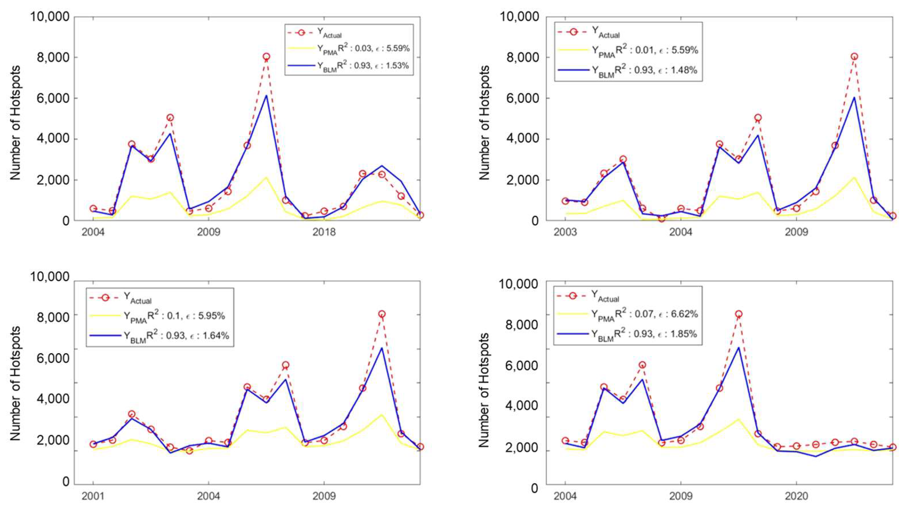
3.2. Evaluation of Bayesian Concept When Used as Robust Model

The Bayesian concept has been known as a concept that can improve model performance, such as a linear regression model, minimizing the distribution of the error value from the model. The Bayesian concept is tested in this research to improve model performance and predict each year’s phenomena. The test is performed using the cross validation principle. A total of C(24,3)-year combinations consisting of training and testing sets were used, with the testing set being the entire combination of data from 3 years taken from 1997 to 2020. The remaining years of each variation were used as training sets consisting of prior and posterior sets. Year selection for use in the posterior process were based on each year’s performance in the Section 3.1 analysis. For example, when used to predict hotspots in 1997, 2001, and 2018, climate and hotspot data from 2003, 2016, and 2007 were used in the posterior process to obtain the BLM model. Meanwhile, the rest of the 18 years of data were used in the prior process to develop the initial model. The performance of the BLM was compared with the model that was developed only using PMA and used all 21 years of training data, except 1997, 2001, and 2018, which were used in the testing data.
There are 2024 combinations of testing and training years with 253 unique models for each year to be tested for regression performance. Figure 6 shows the percentage of the model used to predict each year’s data with a value of R 2 > 0.9 . For example, 72% of PMA models can predict 2002 hotspots with R 2 > 0.9 . Meanwhile, almost 90% of BLM models that predicted hotspots in 2002 have R 2 > 0.9 . This result shows that BLM improved the model’s performance significantly when used to predict hotspots in 2002. Figure 6 shows that the Bayesian concept can massively improve the PMA-based prediction model. Using a few years of data as a data update during the posterior process significantly increases robust model performance. When using the PMA-based model, only 28.65% of the models from the cross validation model managed to have R 2 > 0.9 . Bayesian inference managed to double the model number with R 2 > 0.9 resulting in 61.11% of the total analysed model during cross validation evaluation.
The easiest three years to predict using the BLM model are 2002, 2006, and 2015. There was almost 90% model success in predicting hotspots in those three years with R 2 > 0.9 . In 2002 and 2015, hotspots reached more than 10 thousand during peak months. The result is satisfying, especially when compared to the PMA-based model with a less than 30% model with R 2 > 0.9 . More than 80% of the model also could predict other crucial years, 2004, 2009, and 2019, with more than 8000 hotspots during peak months. This result shows that the algorithm used to build the model is powerful when used to predict a high number of hotspots related to ENSO and IOD, with some exceptions, such as what happened in 1997. Less than 4% of the model accurately predicted hotspots in 1997. This low accuracy is due to the unique characteristic of 1997 events (Figure 7).
Figure 7 shows that wildfires in 1997 happened when Niño3.4 and the DMI index reached a value of more than 1.5, which are far above other years’ indexes, except the DMI index in 2019. However, the number of hotspots in the analysed area is only around 8000, less than the 2002, 2006, and 2015 hotspots. In other years, conditions that resulted in around 8000 hotspots and is easy to predict are moderate El Niño (2004, 2009) and weak El Niño followed by weak IOD+. Since 1997, wildfires happened during extreme El Niño and IOD+, and the model will predict a much higher number of hotspots than in other years, which is inaccurate.
The BLM model was built using relative dry spells that carried ENSO and IOD variability using Equations (9)–(12). Therefore, the model’s performance was highly related to the behaviour of Niño3.4 and DMI indexes. Since the model was optimised to predict a higher number of hotspots, BLM model performance tended to increase when used to predict a high number of hotspots, especially related to ENSO and IOD phenomena. Vice versa, model performance was significantly lower when used to predict wildfire events with low numbers of hotspots, such as 1998, 1999, 2008, 2017, and 2020. Only less than 50% of the models managed to predict hotspots in those five years with R 2 > 0.9 . Regardless, the algorithm in this research is promising for being used in the future. Considering that urgency of modelling the high number of hotspots is much higher than the lower number, the result is satisfying. There is still room for improvement in the model. Therefore, we need to examine some details that may be useful to understand the consequence of using BLM to improve the performance of the PMA-based initial model.

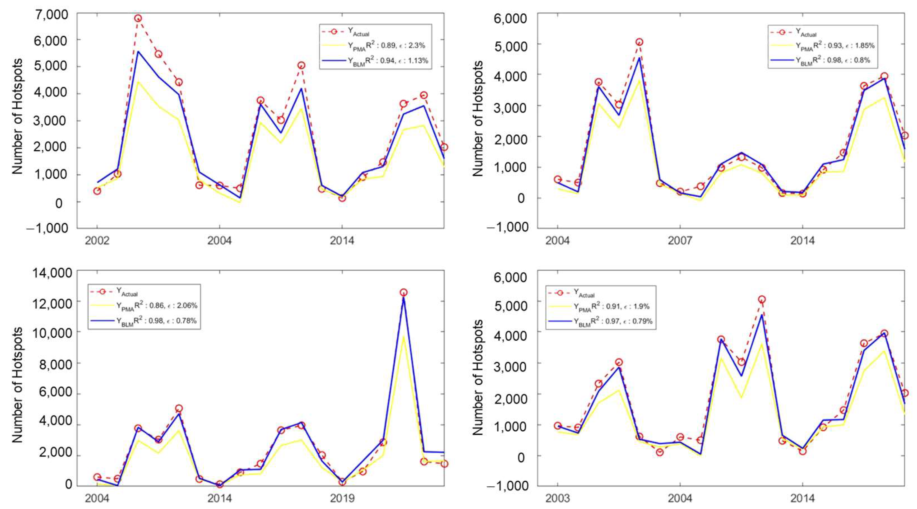
3.2.1. Case Study: Four Models with Highest Values of Coefficient Determination ( R 2 )

All four models with the highest values of R 2 are obtained when 2019 is used in the test data, while the two other years vary in terms of ENSO and IOD. The performance of the BLM is very impressive when used to predict the 2019 hotspot with less than 1.5% error, even more so, considering that 2019 was a unique year with a very strong IOD+ that was only lower than DMI in 1997. Given that hotspots in 1997 had a different character than in other years, making them hard to predict, the prediction results mainly rely on 2002 and 2006 data. Both years had more than 8000 hotspots during the warm phase of ENSO and IOD that co-occurred (Figure 7). However, a case study in Figure 8 did not give a significant improvement in using BLM instead of the PMA-based model, let alone show the significant impact that BLM had. This behaviour is caused by the PMA model already having an R 2 of more than 0.9, except when used to predict 2004, 2005, and 2019 hotspots.
When used to predict 2004, 2005, and 2019 hotspots, the PMA model gives a value of R 2 0.86. BLM manages to improve the value of R 2 to 0.99. This result is quite significant and reveals the potential weakness of the PMA-based model. PMA-based model performance decreases when used to predict three years with more than 2000 hotspots with different characteristics of ENSO and IOD for each year. Therefore, it reduces hotspot variability in the training data. The PMA-based model consistently underestimates hotspots’ numbers each year compared to the actual data. The worst one underestimates hotspots in 2019 by almost 4000 hotspots during the peak wildfire events. During this condition, the use of BLM to improve the model’s performance becomes necessary. BLM managed to increase the model’s accuracy by increasing the predicted hotspots. BLM successfully reduced the error value from 2.63% to 0.88%. The most significant improvement was achieved when BLM accurately predicted 2019 hotspots, especially during peak wildfires.

3.2.2. Case Study: Four Models with Lowest Values of Root Mean Square Error ( R MSE )

The case study in Figure 9 shows that PMA-based models tend to underestimate the actual hotspot number. Meanwhile, BLM consistently manages to increase the predicted hotspot value so that it is closer to the actual hotspots, resulting in a significant reduction of RMSE. The lowest value of RMSE is obtained when the model is used to predict 2004, 2014, and 2019 hotspots. Similar to the previous analysis, the accuracy of the BLM model is very high when used to predict the 2019 hotspot. The difference with the previous analysis appears in the performance of the PMA model, which is noticeably lower than the BLM result.

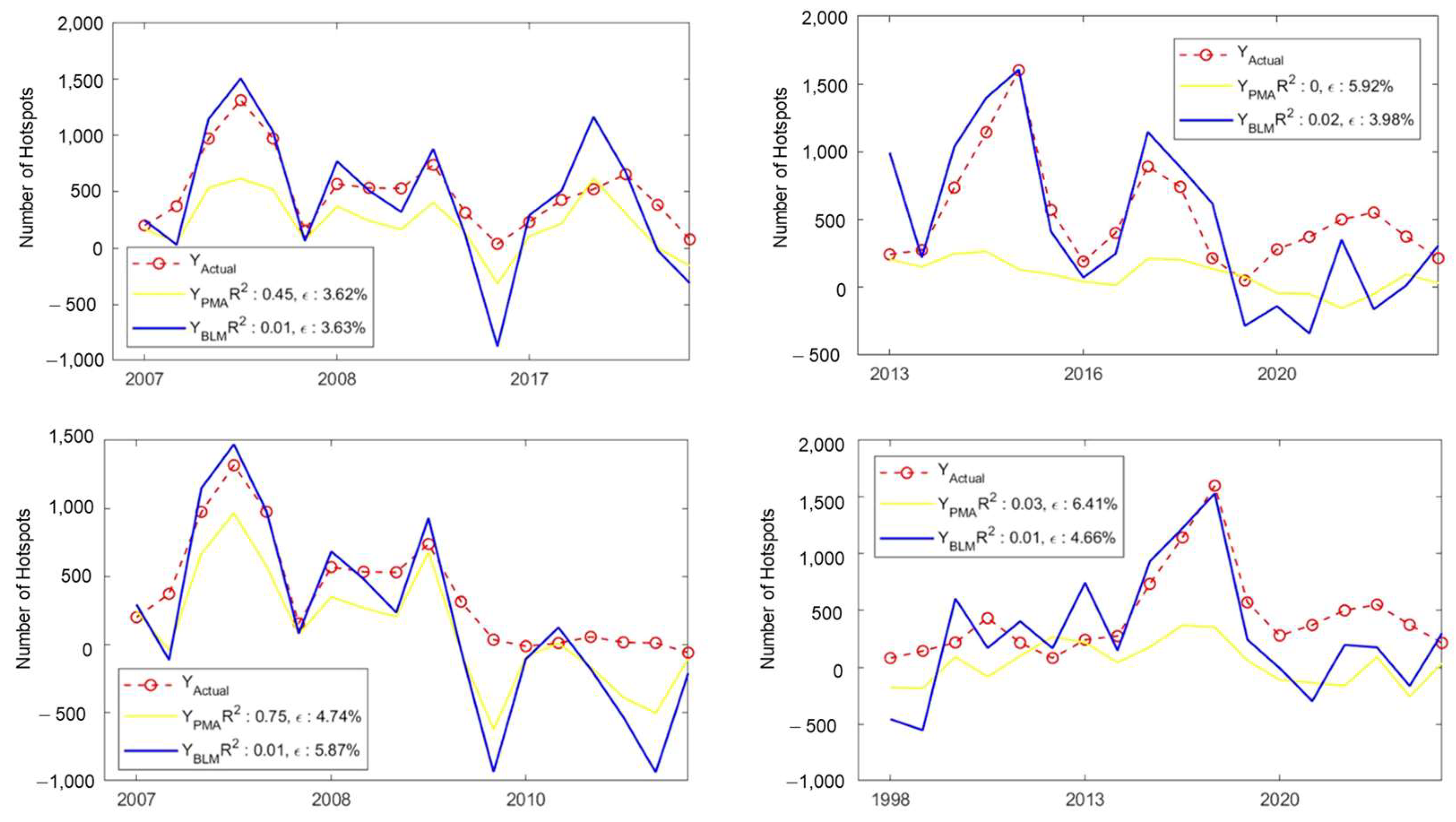
3.2.3. Case Study: Four Models with Lowest Value of Coefficient Determination ( R 2 )

As expected with the performance of the BLM model in Figure 7, both PMA-based and BLM models tend to have lower accuracy when used to predict the lower number of hotspots, especially around 0 hotspot value, such as what happened in 2010. PMA-based and BLM models will result in a negative value when approaching 0 hotspots. Since a negative value of hotspots is not realistic, the negative hotspot value can be seen as 0. Nonetheless, the benefit of using BLM to improve the PMA-based model is noticeable in all case studies in Figure 10. The PMA-based model in Figure 10 significantly underestimates the number of hotspots for each year, especially when estimating 2007, 2013, 2016, and 2020 hotspots. Even though the R 2 values are shallow in all models in Figure 10, we can see that trend of the actual hotspots is closer to the estimation of BLM. By all means, the value of the R 2   in Figure 10 is not acceptable in statistical terms, especially the BLM one. All the R 2 values are close to 0, which makes them not worth considering statistically. However, the error value is still under 7%, especially when it tends to happen during a low number of hotspots. Without question, the model still needs to be improved to mitigate this case if it wants to be used robustly.

3.2.4. Case study: Four Models with Highest Values of Root Mean Square Error ( R MSE )

Results in Figure 11 confirm the previous deduction regarding model performance when used to predict 1997 events. Since the value of Niño3.4 and DMI are far higher than in other years, the models tend to overestimate the actual hotspot value. The BLM model performance in Figure 11 reflects this behaviour. Interestingly, PMA still tends to underestimate the values of the actual hotspots even with powerful El Niño and IOD. In terms of prevention, model performance should underestimate the scale of the events in the future. Underestimating the scale of wildfires can lead to futile prevention efforts if the spread rate becomes out of control. In this regard, using BLM to improve PMA-based models seems necessary to prevent extreme wildfire events in the future during a very long dry season. However, Figure 11 shows the potential flaw when using BLM in the PMA-based models. The case study in Figure 11 shows that BLM gives a lower value of R 2 and a higher value of RMSE. Even though it is highly influenced by miscalculating the 1997 wildfire event, this behaviour must be addressed. Therefore, it can be diagnosed and improved in future research.

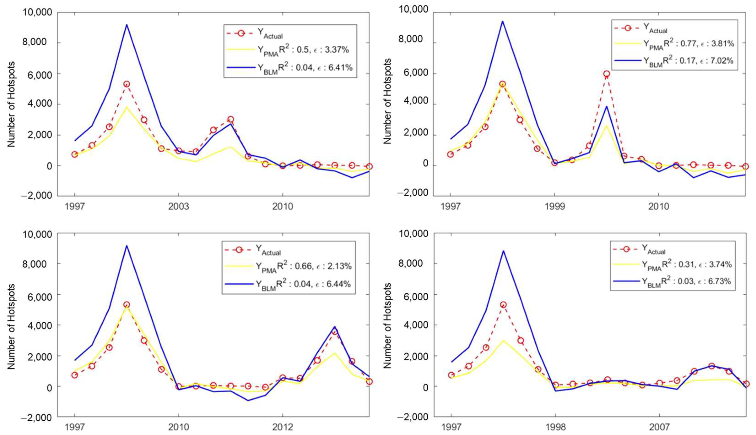
3.2.5. Case Study: Four Models That BLM Failed to Improve

Figure 12 shows that using BLM to improve the PMA-based model does not always provide benefits and reduces the performance of the initial model in some cases. Focused on the 1997 estimation, PMA-based models give superior results compared to BLM in terms of R 2 and RMSE values. Using PMA-based only, all four cases have R 2 values of more than 0.8 with less than 2.5% RMSE. Even though it is not as high as the majority performance of BLM ( R 2 > 0.9), it is much more acceptable than the less than 0.3 values produced by the BLM approach. All models in Section 3.2.1, Section 3.2.2, Section 3.2.3, Section 3.2.4, Section 3.2.5 and Section 3.2.6 show that BLM always gives a higher hotspot estimation than the PMA-based model. Therefore, if the PMA-based model already gives an overestimated result, using BLM in the PMA-based model will give a very overestimated result. Therefore, it reduces the performance of the models and increases the error value of the prediction.

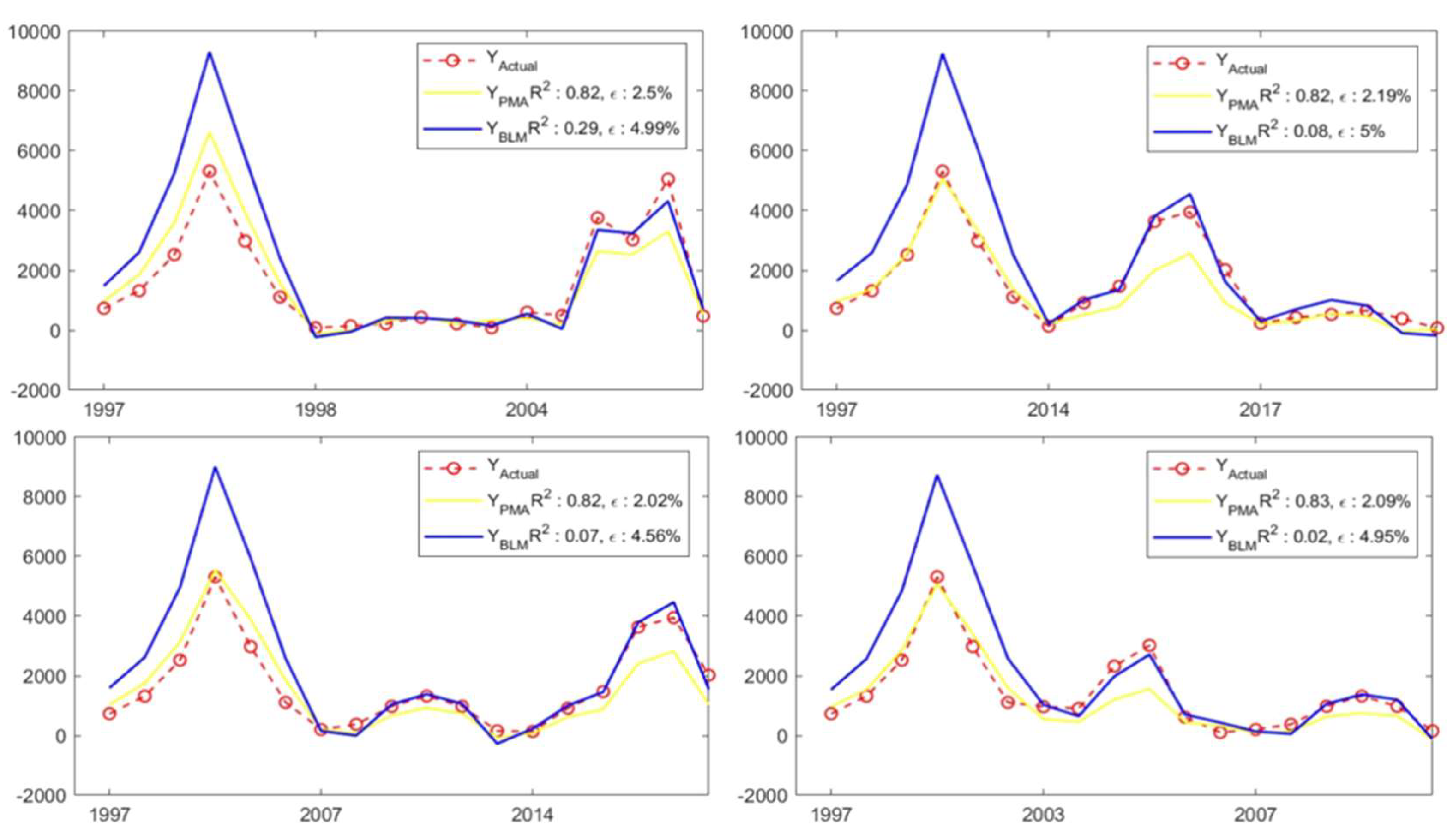
3.2.6. Case Study: Four Models That Necessitate Use of BLM

Since the PMA-based model underestimates the actual hotspot, there is a case in which it results in close to 0 hotspot estimation. As shown in Figure 13, PMA-based models can give completely irrelevant results and should be avoided. Luckily, this happens in years that are known to be dryer than normal. For example, 2004 and 2009 were years with the warm phase of ENSO and IOD during the Kalimantan dry season. Therefore, the result of the prediction model is expected to give a higher number of hotspots than a normal year, not close to 0. Using BLM to improve the model results in a very high estimation accuracy with a value of R 2 > 0.9 and less than 2% RMSE. Therefore, the results of the PMA-based model can be avoided. When the estimation is performed during the dry season, which happen during the warm phase of ENSO and IOD, it is necessary to use BLM in order to improve the performance of the prediction model. This result is in line with the general performance of the model shown in Figure 7.

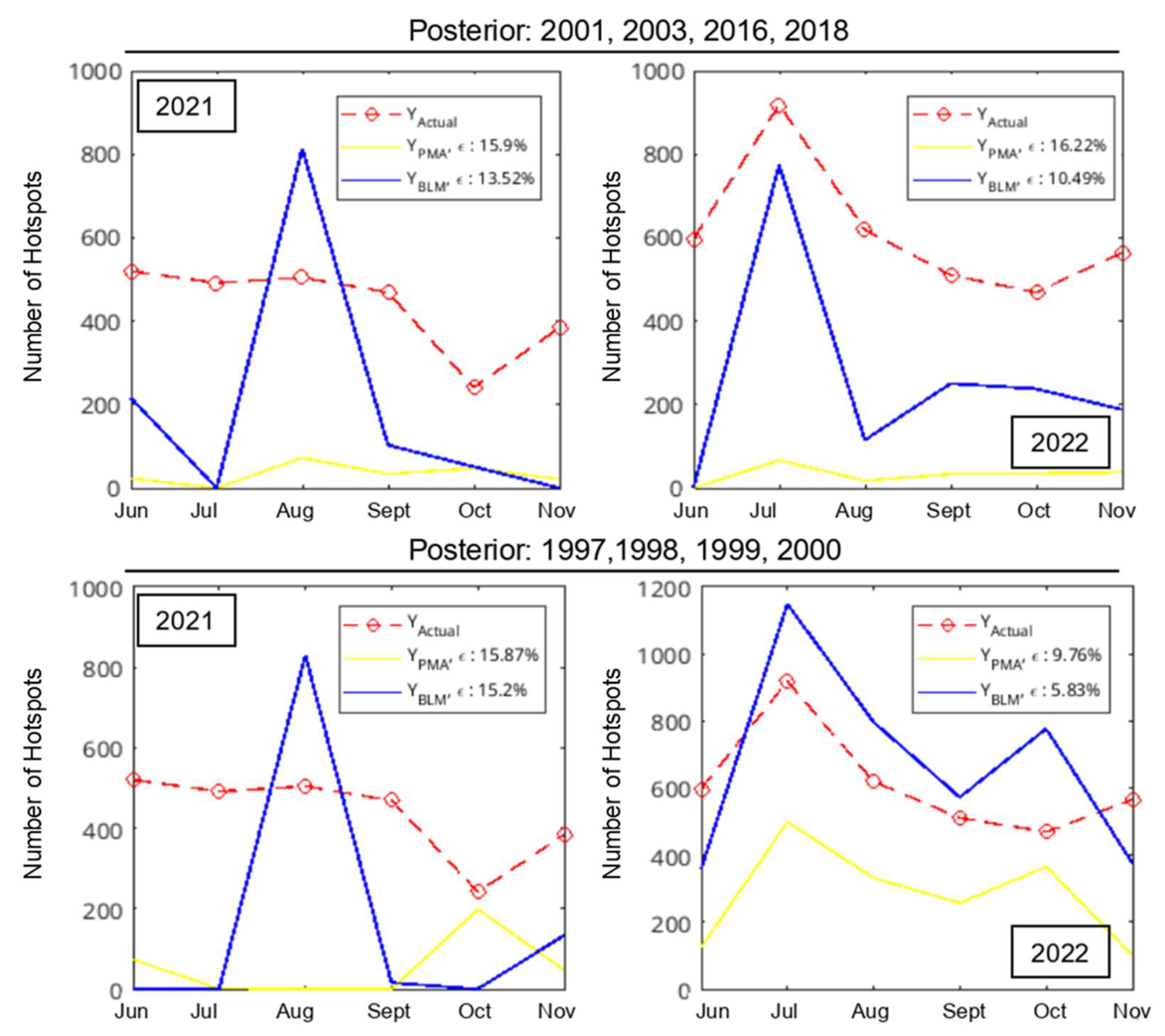
3.3. Estimation of Monthly Hotspots in 2021 and 2022

2021 and 2022 hotspot estimations show exciting results. Using 1997–2000 or 2001, 2003, 2016, and 2018 as a posterior, the 2022 estimation is more accurate than the 2021 estimation. The poor performance, when used to estimate the 2021 hotspot, exhibits the low performance of the model for La Niña years in the cross validation test (Figure 6). 2021 was, in fact, a moderate La Niña year with negative IOD across the whole Kalimantan dry season period. Since the model is built using a logistic function, a negative value of the Niño3.4 index and DMI will result in a close to 0 value of the multiplier. Therefore, the model tends to underestimate the actual hotspots. However, model behaviour is quite different when estimating the 2022 hotspots. Even though both suffered moderate La Niña and negative IOD, the 2022 estimation still carried a similar pattern and resembled the actual hotspot pattern. The model follows Equation (1), which also assumes that drought conditions on one observation grid do not depend on other grids. The results cannot explain the location of hotspots expected to occur because the prediction is only on the total monthly hotspots in the region under study.
Figure 14 shows that hotspots in 2022 were more related to the drought conditions in Kalimantan than hotspots in 2021. Hotspot occurrence and patterns in 2021 did not follow the drought condition pattern. This result indicates that hotspots in 2021 were triggered and affected by another factor, such as deforestation. Although all estimations in Figure 14 show the low value of R 2 , using BLM to predict 2022 hotspots resulted in less than a 10% off error value. Another step that can be used to increase the accuracy is by changing the posterior data characteristic. Using a high number of hotspots in the posterior (1997–2000 data) increases the accuracy of the 2022 estimation but decreases the accuracy of the 2021 estimation. This result shows that separating data as prior and posterior is essential to obtain the best results.

4. Discussion

Analysis in Section 3 proves that Kalimantan has high variability of wildfire events [8,9,54], which makes it hard to model. The high variability of wildfires in Kalimantan was influenced by many climate indicators that affect dry season conditions for each year [55,56]. The analysed region itself can still be divided into two areas that have monsoonal and equatorial precipitation patterns [57]. Both are different since areas with equatorial precipitation patterns tend to have much shorter dry seasons [58]. Areas with equatorial precipitation patterns have two dry seasons in one year with a duration of about 2–3 months each, while areas with the monsoonal pattern only have one annual dry season of around six months duration [59]. On top of that, there are a lot of other local and climate indicators that influence the start and duration of the dry season, such as local sea surface temperature [3], Inter Tropical Convergence Zone (ICTZ) signal [58], IOD [59], and ENSO [8].
In general, using Bayesian inference to improve the model’s performance give significant result compared to the method from previous research, which only uses PMA. Focused on only ENSO [60] and IOD [61] as two sources of high climate variability, models can perform well when used to estimate more significant wildfire events with a higher number of hotspots [23], primarily when related to the occurrence of El Niño and IOD+ phenomena [23]. We defined model performance as “great” when the value of R 2 > 0.9 during testing data estimation. When used to estimate wildfires in a normal year (1998, 1999, 2001, 2003, 2010, 2012, 2013) [54], there is around a 60% chance that the models perform well, except in 1999, with only less than 30%. The model’s performance is quite similar when estimating weak El Niño and normal IOD conditions (2004, 2014, 2018) [54], with around a 60% chance of excellent performance using a different combination of prior and posterior. This behaviour is in line with previous research showing that wildfire variability during weak El Niño and normal IOD is quite similar to normal conditions [54].
Performance of the model significantly improved when used to estimate hotspots in weak El Niño and IOD+ years (2006, 2019) and moderate El Niño and normal IOD (2002, 2009), as well as very strong El Niño and IOD+ (2015) except the 1997 wildfires. This result confirmed previous research results showing that 1997 wildfire events differed from other years [54], which this research cannot address. Therefore, it is hard to model using a method mainly affected by the variability of other years. Considering that the model’s urgency rises following the increase of extreme dry season probability as an impact of global warming, a model with higher performance in extremely dry conditions is much preferable. This research nullifies previous method flaws in [23] that provide lower performance when used to estimate hotspots related to the powerful El Niño and IOD+ in 2015. However, it creates another flaw that needs to be improved regarding the model’s behaviour. The BLM method is prone to giving an overestimated result compared to the actual hotspot. Even though it is suitable for prevention rather than underestimating results, too high of an overestimation can create a waste of resources used to mitigate disasters.
PMA-based and BLM models are developed using dry spells relative to and precipitation of each analysed grid as independent variables, while hotspots are used as dependent variables. Following Equation (1), the assumption that drought conditions in one observation grid are independent of other observation grids is formed automatically. The benefit of using this approach is that we can slightly ignore different precipitation patterns explained previously. However, the downside is that we cannot locate where the estimated hotspot will occur since we only predict the total monthly hotspots in the analysed region. Moreover, we can agree that different characteristic data in the posterior estimation influence the accuracy of the final results. Therefore, we suggest using a combination of posterior when estimating upcoming hotspot events and treating them as a different model so that we can follow the dominant property of the prediction results.

Wildfire Characteristics in 2006, 2013, and 2019

2006, 2013, and 2019 are the only years with a lower performance value than average when used to estimate hotspots from 1997–2000. Using 2013′s characteristics as posterior can lead to a massive decrease in overall model performance. During mid-2013, there were Madden Julian Oscillation (MJO) anomalies [62,63] affecting the dry season in the western part of Kalimantan [64]. During phases 5–8, MJO could increase the fire detection ratio compared to phases 1–4 [65] in western Kalimantan. Since the MJO phase has quite a short duration, MJO variability is often suppressed by other more immense climate variabilities, such as ENSO and IOD. Therefore, MJO characteristics in the Kalimantan hotspot are almost invisible. The variability is only noticeable when there is a significant anomaly, such as what happened in 2013.
Different from 2013, 2006 and 2019, dry seasons were mainly driven by El Niño and IOD+, which happened simultaneously [64]. However, both years did not have similar characteristics. Two thousand six wildfires happened during the weak El Niño followed by IOD+. Individually, the impact of both phenomena is relatively low in Kalimantan [66,67]. The joint impact of both phenomena produces many hotspots, resulting in a very long dry season [68,69].
Meanwhile, 2019’s wildfires were mainly driven by strong IOD+ that have never happened for the last 20 years. During 2019′s wildfire event, ENSO was in normal condition. Some ENSO indexes show that it already passed the boundary to become El Niño, but the strength of 2019′s El Niño was very weak. The difference in IOD+ strength in 2006 and 2019 produced some uniqueness to the characteristics of both years. Therefore, both years are necessary to be used in the initial model (prior) to increase the variability of hotspots that can be modelled.

5. Conclusions

Kalimantan has high variability of dry season influenced by both local and global climate indicators. This high variability causes Kalimantan to have different starts and durations of the dry season each year. Therefore, developing a hotspot prediction model that performs robustly is more challenging. Using the Bayesian concept to improve the previous method (PMA-based model) significantly increases accuracy, especially during extremely dry conditions such as during strong El Niño or/and strong IOD+. However, overall model performance is still low when estimating years with less dry conditions and only produces a low number of hotspots. Even so, this result is still promising since the model is developed mainly to anticipate extreme dry conditions as an impact of ENSO or/and IOD in the future.
Because it is focused on ENSO or/and IOD impact on dry seasons and hotspots, the model accuracy increases following the strength of El Niño or/and IOD+. Therefore, the model will suffer when used to predict hotspots in the dry season driven by other climate factors, such as MJO. The last thing that needs to be addressed in future research is that the Bayesian model in this research is prone to overestimating the number of hotspots. Although it is better for prevention than underestimating, it can result in wasting resources to anticipate disasters.

Author Contributions

Conceptualization, S.N., P.S. and A.S.; methodology, A.S. and P.S.; software, E.A., M.K.N. and P.S.; validation, S.N., A.S. and P.S.; formal analysis, S.N., P.S. and E.A.; investigation, A.S.; resources, S.N. and A.S.; data curation, E.A. and M.K.N.; writing—original draft preparation, E.A. and P.S.; writing— review and editing, E.A., P.S. and S.N.; visualization, E.A.; supervision, S.N. and A.S.; project administration, S.N. All authors have read and agreed to the published version of the manuscript.

Funding

This research was funded Directorate General of Higher Education, Ministry of Education, Culture, Research, and Technology under the “Hibah Penelitian Tesis Magister” scheme for budget year 2022. Number: 082/E5/PG.02.00.PT/2022, sub-number: 3864/IT3.L1/PT.01.03/P/B/2022.

Institutional Review Board Statement

Not applicable.

Informed Consent Statement

Not applicable.

Data Availability Statement

Not applicable.

Acknowledgments

The authors would like to thank Department of Mathematics, IPB University and Meteorological, Climatological and Geophysical Agency (BMKG) for their invaluable support and assistance throughout this research.

Conflicts of Interest

The authors declare no conflict of interest.

References

  1. Nurdiati, S.; Bukhari, F.; Julianto, M.T.; Najib, M.K.; Nazria, N. Heterogeneous Correlation Map Between Estimated ENSO And IOD From ERA5 And Hotspot In Indonesia. Jambura Geosci. Rev. 2021, 3, 65–72. [Google Scholar] [CrossRef]
  2. Shafitri, L.D.; Prestyo, Y.; Hani’ah. Analysis of Forest Deforestation in Riau Province Using Polarimetric Method in Remote Sensing. J. Geod. Undip. 2018, 7, 212–222. (In Indonesian) [Google Scholar]
  3. Dafri, M.; Nurdiati, S.; Sopaheluwakan, A. Quantifying ENSO and IOD Impact to Hotspot in Indonesia Based on Heterogeneous Correlation Map (HCM). J. Phys. Conf. Ser. 2021, 1869, 012150. [Google Scholar] [CrossRef]
  4. Atmadja, S.; Indriatmoko, Y.; Utomo, N.A.; Komalasari, M.; Ekaputri, A.D. Kalimantan Forests and Climate Partnership, Central Kalimantan, Indonesia. In REDD+ on the Ground: A Case Book of Subnational Initiatives across the Globe; Sills, E.O., Ed.; Center for International Forestry Research (CIFOR): Bogor, Indonesia, 2015; pp. 290–308. [Google Scholar]
  5. Ministry of Environment and Forestry of The Republic of Indonesia Sipongi.menhlk.go.id. Available online: Sipongi.menhlk.go.id (accessed on 30 November 2022).
  6. Santriwati, S.; Halide, H.; Hasanuddin, H. Oceanic-Atmospheric Factors to Predict Hostspots in the Southern Southeast Asia Region. J. Geocelebes 2021, 5, 116–130. (In Indonesian) [Google Scholar] [CrossRef]
  7. Candra, A.; Thamrin, M. Analysis of the Influence of Climate Factors and Forest/Land Fires on Pm10 Concentrations in Pekanbaru City During the Period of 2011–2015. Ilmu Lingkung. 2017, 11, 209–227. (In Indonesian) [Google Scholar] [CrossRef]
  8. Najib, M.K.; Nurdiati, S.; Sopaheluwakan, A. Copula-Based Joint Distribution Analysis of the ENSO Effect on the Drought Indicators over Borneo Fire-Prone Areas. Model. Earth Syst. Environ. 2022, 8, 2817–2826. [Google Scholar] [CrossRef]
  9. Endrawati, E. Identification of Forest and Land Fire Scars Using Semi-Automated Analysis of Landsat Satellite Imagery. Semin. Nas. Geomatika 2018, 2, 273. (In Indonesian) [Google Scholar] [CrossRef] [Green Version]
  10. Samsuri, A.; Zaitunah, O.R. Green Open Space Needs Analysis: Oxygen Demand Approach. J. Silva Trop. 2021, 5, 305–320. (In Indonesian) [Google Scholar]
  11. Fanin, T.; Van Der Werf, G.R. Precipitation-Fire Linkages in Indonesia (1997–2015). Biogeosciences 2017, 14, 3995–4008. [Google Scholar] [CrossRef] [Green Version]
  12. Gutierrez, A.A.; Hantson, S.; Langenbrunner, B.; Chen, B.; Jin, Y.; Goulden, M.L.; Randerson, J.T. Wildfire response to changing daily temperature extremes in California’s Sierra Nevada. Sci. Adv. 2021, 7, eabe6417. [Google Scholar] [CrossRef]
  13. Supari; Tangang, F.; Juneng, L.; Aldrian, E. Observed changes in extreme temperature and precipitation over Indonesia. Int. J. Climatol. 2017, 37, 1979–1997. [Google Scholar] [CrossRef]
  14. Wahyuni, H.; Suranto, S. The Impact of Large-Scale Deforestation on Global Warming in Indonesia. JIIP J. Ilm. Ilmu Pemerintah. 2021, 6, 148–162. (In Indonesian) [Google Scholar] [CrossRef]
  15. Handoko, E.Y.; Filaili, R.B.; Yuwono. Analysis of the Enso Phenomenon in Indonesian Waters Using Topex/Poseidon and Jason Series Altimetry Data 1993–2018. Geoid 2019, 14, 43. (In Indonesian) [Google Scholar] [CrossRef] [Green Version]
  16. Hidayat, A.M.; Efendi, U.; Agustina, L.; Winarso, P.A. Correlation of Niño 3.4 Index and Southern Oscillation Index (Soi) with Rainfall Variation in Semarang. J. Sains Teknol. Modif. Cuaca 2018, 19, 75. (In Indonesian) [Google Scholar] [CrossRef]
  17. Abram, N.J.; Wright, N.M.; Ellis, B.; Dixon, B.C.; Wurtzel, J.B.; England, M.H.; Ummenhofer, C.C.; Philibosian, B.; Cahyarini, S.Y.; Yu, T.L.; et al. Coupling of Indo-Pacific Climate Variability over the Last Millennium. Nature 2020, 579, 385–392. [Google Scholar] [CrossRef]
  18. Saji, N.H.; Goswami, B.N.; Vinayachandran, P.N.; Yamagata, T. A Dipole Mode in the Tropical Indian Ocean. Nature 1999, 401, 360–363. [Google Scholar] [CrossRef]
  19. Kertayasa, I.M.; Sukarasa, I.K.; Widagda, I.G.A.; Hendrawan, I.G. Effect of Indian Ocean Dipole Mode (Iodm) on Rain Intensity in the Western Indonesian Maritime Continent (Bmi). Buletin Fisika 2013, 14, 25–30. (In Indonesian) [Google Scholar]
  20. Nur’utami, M.N.; Hidayat, R. Influences of IOD and ENSO to Indonesian Rainfall Variability: Role of Atmosphere-Ocean Interaction in the Indo-Pacific Sector. Procedia Environ. Sci. 2016, 33, 196–203. [Google Scholar] [CrossRef] [Green Version]
  21. Najib, M.K.; Nurdiati, S.; Sopaheluwakan, A. Multivariate Fire Risk Models Using Copula Regression in Kalimantan, Indonesia. Nat. Hazards 2022, 113, 1263–1283. [Google Scholar] [CrossRef]
  22. Nurdiati, S.; Sopaheluwakan, A.; Septiawan, P. Spatial and Temporal Analysis of El Niño Impact on Land and Forest Fire in Kalimantan and Sumatra. Agromet 2021, 35, 1–10. [Google Scholar] [CrossRef]
  23. Nurdiati, S.; Sopaheluwakan, A.; Julianto, M.T.; Septiawan, P.; Rohimahastuti, F. Modelling and Analysis Impact of El Niño and IOD to Land and Forest Fire Using Polynomial and Generalized Logistic Function: Cases Study in South Sumatra and Kalimantan, Indonesia. Model. Earth Syst. Environ. 2022, 8, 3341–3356. [Google Scholar] [CrossRef]
  24. Sang, Y.F.; Singh, V.P.; Xu, K. Evolution of IOD-ENSO Relationship at Multiple Time Scales. Theor. Appl. Climatol. 2019, 136, 1303–1309. [Google Scholar] [CrossRef]
  25. Cane, M.A. The Evolution of El Niño, Past and Future. Earth Planet. Sci. Lett. 2005, 230, 227–240. [Google Scholar] [CrossRef]
  26. Suhermat, M.; Dimyati, M.; Supriatna, S.; Martono, M. Impact of Climate Change on Sea Surface Temperature and Chlorophyll-a Concentration in South Sukabumi Waters. J. Ilmu Lingkung. 2021, 19, 393–398. [Google Scholar] [CrossRef]
  27. Zhang, Y.; Du, Y. Extreme IOD Induced Tropical Indian Ocean Warming in 2020. Geosci. Lett. 2021, 8, 37. [Google Scholar] [CrossRef]
  28. Muttalib, A.M.A.; Ameen, S.M.M.; Mahmood, A.B. The Impacts of ENSO and IOD on the MSL of the Arabian Gulf and the Arabian Sea by Using Satellite Altimetry Data. Ilmu Kelaut. Indones. J. Mar. Sci. 2021, 26, 143–147. [Google Scholar] [CrossRef]
  29. Cai, W.; Santoso, A.; Collins, M.; Dewitte, B.; Karamperidou, C.; Kug, J.S.; Lengaigne, M.; McPhaden, M.J.; Stuecker, M.F.; Taschetto, A.S.; et al. Changing El Niño–Southern Oscillation in a Warming Climate. Nat. Rev. Earth Environ. 2021, 2, 628–644. [Google Scholar] [CrossRef]
  30. Nikonovas, T.; Spessa, A.; Doerr, S.H.; Clay, G.D.; Mezbahuddin, S. ProbFire: A probabilistic fire early warning system for Indonesia, Nat. Hazards Earth Syst. Sci. 2022, 22, 303–322. [Google Scholar] [CrossRef]
  31. Ardiansyah, M.; Boer, R.; Situmorang, A.P. Typology of Land and Forest Fire in South Sumatra, Indonesia Based on Assessment of MODIS Data. IOP Conf. Ser. Earth Environ. Sci. 2017, 54, 012058. [Google Scholar] [CrossRef]
  32. Sabani, W.; Rahmadewi, D.P.; Rahmi, K.I.N.; Priyatna, M.; Kurniawan, E. Utilization of MODIS Data to Analyze the Forest/Land Fires Frequency and Distribution (Case Study: Central Kalimantan Province). IOP Conf. Ser. Earth Environ. Sci. 2019, 243, 012032. [Google Scholar] [CrossRef]
  33. Aisyah, S.; Simaremare, A.A.; Adytia, D.; Aditya, I.A.; Alamsyah, A. Exploratory Weather Data Analysis for Electricity Load Forecasting Using SVM and GRNN, Case Study in Bali, Indonesia. Energies 2022, 15, 3566. [Google Scholar] [CrossRef]
  34. Nurdiati, S.; Sopaheluwakan, A.; Najib, M.K. Statistical Bias Correction for Predictions of Indian Ocean Dipole Index with Quantile Mapping Approach. In Proceedings of the 1st Int’ Conference on Sccience and Mathemtics (IMC-SciMath), Parapat, Indonesia, 9–11 October 2019. [Google Scholar]
  35. Najib, M.K.; Nurdiati, S. Statistical Bias Correction on Predicted Sea Surface Temperature Data in the Western and Eastern Indian Ocean Dipole Regions. Jambura Geosci. Rev. 2021, 3, 9–17. (In Indonesian) [Google Scholar] [CrossRef]
  36. Morales-Velázquez, M.I.; Herrera, G.D.S.; Aparicio, J.; Rafieeinasab, A.; Lobato-Sánchez, R. Evaluating Reanalysis and Satellite-Based Precipitation at Regional Scale: A Case Study in Southern Mexico. Atmósfera 2021, 34, 189–206. [Google Scholar] [CrossRef]
  37. Liu, J.; Zhou, Y.; Lu, F.; Yu, Y.; Yan, D.; Hu, Y.; Xue, W. Evaluating satellite- and reanalysis-based precipitation products over the Qinghai-Tibetan Plateau in the perspective of a new error-index system. Int. J. Climatol. 2022, 2022, 1–20. [Google Scholar] [CrossRef]
  38. Hassan, J.O.; Amer, S.M. Evaluation of satellite-based and reanalysis precipitation datasets by hydrologic simulation in the Chenab river basin. J. Water Clim. Chang. 2022, 13, 1563–1582. [Google Scholar] [CrossRef]
  39. Hersbach, H.; Bell, B.; Berrisford, P.; Horányi, A.; Muñoz, J.; Sabater.; Nicolas, J.; Radu, R.; Schepers, D.; Simmons, A.; et al. Global Reanalysis: Goodbye ERA-Interim, Hello ERA5. ECMWF Newsl. 2019, 159, 17–24. [Google Scholar]
  40. Rizani, M.; Fathurrahmani, F. Web-based Day Without Rain (HTH) Monitoring Application at Banjarbaru Class 1 Climatology Station. J. Sains Dan Inform. 2018, 4, 63–72. (In Indonesian) [Google Scholar] [CrossRef] [Green Version]
  41. He, B.; Zhong, Z.; Chen, D.; Liu, J.; Chen, Y.; Miao, C.; Ding, R.; Yuan, W.; Guo, L.; Huang, L.; et al. Lengthening dry spells intensify summer heatwaves. Geophys. Res. Lett. 2022, 49, e2022GL099647. [Google Scholar] [CrossRef]
  42. Groisman, P.Y.; Knight, R.W. Prolonged dry episodes over the conterminous United States: New tendencies emerging during the last 40 years. J. Clim. 2008, 21, 1850–1862. [Google Scholar] [CrossRef]
  43. Brunetti, M.; Maugeri, M.; Monti, F.; Nanni, T. Changes in daily precipitation frequency and distribution in Italy over the last 120 years. J. Geophys. Res. 2004, 109, D05102. [Google Scholar] [CrossRef]
  44. Palmer, P.B.; O’Connell, D.G. Research Corner: Regression Analysis for Prediction: Understanding the Process. Cardiopulm. Phys. Ther. J. 2009, 20, 23–26. [Google Scholar] [CrossRef] [PubMed]
  45. Dimitriadou, S.; Nikolakopoulos, K.G. Multiple Linear Regression Models with Limited Data for the Prediction of Reference Evapotranspiration of the Peloponnese, Greece. Hydrology 2022, 9, 124. [Google Scholar] [CrossRef]
  46. Manoj, S.; Valliyammai, C.; Kalyani, V. Multivariate Regression Analysis of Climate Indices for Forecasting the Indian Rainfall. Lect. Notes Netw. Syst. 2020, 107, 713–720. [Google Scholar] [CrossRef]
  47. Kalyani, V.; Valliyammai, C.; Manoj, S. Multivariate Regression Analysis on Climate Variables for Weather Forecasting in Indian Subcontinent. Adv. Intell. Syst. Comput. 2020, 1118, 621–628. [Google Scholar] [CrossRef]
  48. Xie, Q.; Tang, L.; Li, W.; John, V.; Hu, Y. Principal Model Analysis Based on Partial Least Squares. arXiv 2019, arXiv:1902.02422. [Google Scholar] [CrossRef]
  49. Abdi, H.; Williams, L.J. Partial Least Squares Methods: Partial Least Squares Correlation and Partial Least Square Regression. Methods Mol. Biol. NeuroImage 2013, 930, 549–579. [Google Scholar]
  50. Chen, C.; Cao, X.; Tian, L. Partial Least Squares Regression Performs Well in MRI-Based Individualized Estimations. Front. Neurosci. 2019, 13, 1282. [Google Scholar] [CrossRef] [Green Version]
  51. Box, G.E.P.; Tiao, G.C. Bayesian Inference in Statistical Analysis; John Wiley & Sons: Hoboken, NJ, USA, 1992; ISBN 9781118033197. [Google Scholar]
  52. Hulu, S.; Sihombing, P.; Sutarman. Analysis of Performance Cross Validation Method and K-Nearest Neighbor in Classification Data. Int. J. Res. Rev. 2020, 7, 69–73. [Google Scholar]
  53. Wright, S. Correlation and causation. J. Agric. Res. 1921, 20, 7. [Google Scholar]
  54. Nurdiati, S.; Bukhari, F.; Julianto, M.T.; Sopaheluwakan, A.; Aprilia, M.; Fajar, I.; Najib, M.K.; Septiawan, P. The Impact of El Niño Southern Oscillation and Indian Ocean Dipole on the Burned Area in Indonesia. Terr. Atmos. Ocean. Sci. 2022, 33, 16. [Google Scholar] [CrossRef]
  55. Nurdiati, S.; Sopaheluwakan, A.; Septiawan, P.; Ardhana, M.R. Joint Spatio-Temporal Analysis of Various Wildfire and Drought Indicators in Indonesia. Atmosphere 2022, 13, 1591. [Google Scholar] [CrossRef]
  56. Safril, A. Rainfall Variability Study in Kalimantan as an Impact of Climate Change and El Niño. AIP Conf. Proc. 2021, 2320, 040002. [Google Scholar] [CrossRef]
  57. Lee, H.S. General Rainfall Patterns in Indonesia and the Potential Impacts of Local Seas on Rainfall Intensity. Water 2015, 7, 1751–1768. [Google Scholar] [CrossRef]
  58. Mcbride, J.L.; Sahany, S.; Hassim, M.E.E.; Nguyen, C.M.; Lim, S.-Y.; Rahmat, R.; Cheong, W.-K. The 2014 Record Dry Spell at Singapore: An Intertropical Convergence Zone (ITCZ) Drought. Bull. Am. Meteorol. Soc. 2015, 96, S126–S130. [Google Scholar] [CrossRef]
  59. Hendrawan, I.G.; Asai, K.; Triwahyuni, A.; Valentina Lestari, D. The Interanual Rainfall Variability in Indonesia Corresponding to El Niño Southern Oscillation and Indian Ocean Dipole. Acta Oceanol. Sin. 2019, 38, 57–66. [Google Scholar] [CrossRef]
  60. Yun, K.-S.; Lee, J.-Y.; Timmermann, A.; Stein, K.; Stuecker, M.F.; Fyfe, J.C.; Chung, E.-S. Increasing ENSO–Rainfall Variability Due to Changes in Future Tropical Temperature–Rainfall Relationship. Commun. Earth Environ. 2021, 2, 43. [Google Scholar] [CrossRef]
  61. Cai, W.; Zheng, X.-T.; Weller, E.; Collins, M.; Cowan, T.; Lengaigne, M.; Yu, W.; Yamagata, T. Projected Response of the Indian Ocean Dipole to Greenhouse Warming. Nat. Geosci. 2013, 6, 999–1007. [Google Scholar] [CrossRef]
  62. Nurdiati, S.; Sopaheluwakan, A.; Septiawan, P. Joint Distribution Analysis of Forest Fires and Precipitation in Response to ENSO, IOD, and MJO (Study Case: Sumatra, Indonesia). Atmosphere 2022, 13, 537. [Google Scholar] [CrossRef]
  63. Kusumaningtyas, S.D.A.; Aldrian, E. Impact of the June 2013 Riau Province Sumatera Smoke Haze Event on Regional Air Pollution. Environ. Res. Lett. 2016, 11, 075007. [Google Scholar] [CrossRef]
  64. Zhang, C. Madden–Julian Oscillation: Bridging Weather and Climate. Bull. Am. Meteorol. Soc. 2013, 94, 1849–1870. [Google Scholar] [CrossRef]
  65. Reid, J.S.; Xian, P.; Hyer, E.J.; Flatau, M.K.; Ramirez, E.M.; Turk, F.J.; Sampson, C.R.; Zhang, C.; Fukada, E.M.; Maloney, E.D. Multi-Scale Meteorological Conceptual Analysis of Observed Active Fire Hotspot Activity and Smoke Optical Depth in the Maritime Continent. Atmos. Chem. Phys. 2012, 12, 2117–2147. [Google Scholar] [CrossRef] [Green Version]
  66. Kurniadi, A.; Weller, E.; Min, S.-K.; Seong, M.-G. Independent ENSO and IOD Impacts on Rainfall Extremes over Indonesia. Int. J. Climatol. 2021, 41, 3540–3656. [Google Scholar] [CrossRef]
  67. As-Syakur, A.R.; Adnyana, I.W.S.; Mahendra, M.S.; Wayan, I.A.; Merit, I.N.; Kasa, I.W.; Ekayanti, N.W.; Nuarsa, I.W.; Sunarta, I.N. Observation of Spatial Patterns on the Rainfall Response to ENSO and IOD over Indonesia Using TRMM Multisatellite Precipitation Analysis (TMPA). Int. J. Climatol. 2014, 34, 3825–3839. [Google Scholar] [CrossRef]
  68. Iskandar, I.; Lestrai, D.O.; Nur, M. Impact of El Niño and El Niño Modoki Events on Indonesian Rainfall. Makara J. Sci. 2019, 23, 7. [Google Scholar] [CrossRef] [Green Version]
  69. Lestari, D.O.; Sutriyono, E.; Sabaruddin; Iskandar, I. Respective Influences of Indian Ocean Dipole and El NiñoSouthern Oscillation on Indonesian Precipitation. J. Math. Fundam. Sci. 2018, 50, 257–272. [Google Scholar] [CrossRef] [Green Version]
Figure 1. Recapitulation of the area on 5 islands affected by wildfires (ha) in Indonesia in 2017–2021.
Atmosphere 14 00286 g001
Figure 2. Monthly hotspots of Kalimantan, Niño3.4 index, DMI index (2001–2020).
Atmosphere 14 00286 g002
Figure 3. Research area with spatial and temporal filters.
Atmosphere 14 00286 g003
Figure 4. Visualization of the Leave p Out Cross Validation with p = 3 .
Atmosphere 14 00286 g004
Figure 5. Performance of each year when used as data update in posterior model.
Atmosphere 14 00286 g005
Figure 6. Performance of PMA-based model and BLM model when used to predict each year’s hotspots.
Atmosphere 14 00286 g006
Figure 7. Performance of Bayesian linear model when used to predict each year’s hotspots.
Atmosphere 14 00286 g007
Figure 8. Performance of Bayesian linear model when used to predict each year’s (June–November) hotspots.
Atmosphere 14 00286 g008
Figure 9. Performance of Bayesian linear model when used to predict each year’s (June–November) hotspots.
Atmosphere 14 00286 g009
Figure 10. Performance of Bayesian linear model when used to predict each year’s (June–November) hotspots.
Atmosphere 14 00286 g010
Figure 11. Performance of Bayesian linear model when used to predict each year’s (June–November) hotspots.
Atmosphere 14 00286 g011
Figure 12. Performance of Bayesian linear model when used to predict each year’s (June-November) hotspots.
Atmosphere 14 00286 g012
Figure 13. Performance of Bayesian linear model when used to predict each year’s (June–November) hotspots.
Atmosphere 14 00286 g013
Figure 14. 2021 and 2022 hotspot estimation using PMA and BLM.
Atmosphere 14 00286 g014
Disclaimer/Publisher’s Note: The statements, opinions and data contained in all publications are solely those of the individual author(s) and contributor(s) and not of MDPI and/or the editor(s). MDPI and/or the editor(s) disclaim responsibility for any injury to people or property resulting from any ideas, methods, instructions or products referred to in the content.

