Extreme Rainfall in Southern Burkina Faso, West Africa: Trends and Links to Atlantic Sea Surface Temperature

Abstract

Understanding the space-time variations of extreme rainfall plays an important role in the management of water-related disasters in Sahel countries. This study investigates temporal changes in rainfall characteristics and explores the link between Atlantic Sea surface temperature and extreme rainfall in the southern part of Burkina Faso. We find substantial spatial heterogeneity in rainfall trends across the study area. In contrast to national and supra-national studies that found predominantly increasing trends in extreme rainfall, we detect more downward than upward trends, particularly for indices representing extreme rainfall. This difference is presumably a consequence of the high spatial variability in rainfall trends that can only be detected with sufficiently dense climate networks. We use the Poisson-General Pareto (Poisson-GP) distribution to quantify the frequency and intensity of extreme rainfall. Our comparison of the traditional, stationary Poisson-GP model with the nonstationary version where rainfall depends on Atlantic SST shows that the nonstationary model outperforms the traditional approach. This finding suggests that the assumption of stationary nature must be considered with care when modeling the frequency and intensity of extreme rainfall in the study area. Overall, our results suggest that the recent increase in flood disasters in Burkina Faso is rather caused by land use and land cover changes and population and urban growth and not by increasing rainfall extremes.

1. Introduction

In recent decades, heavy rainfall has been the main driver of numerous flood disasters in the Sahelian countries of West Africa, with enormous consequences for people and their properties [1]. In Burkina Faso the occurrence of (riverine and flash) floods has increased significantly to five flood events per year during the decade of 2006–2016 compared to one event per year in the period of 1986–2005 [2,3]. For instance, from June to September 2009, flood events affected 512 031 and killed 22 people in the Sahelian countries of West Africa, including Burkina Faso [4]. During the same year, Burkina Faso experienced unprecedented flooding that affected the city of Ouagadougou and the surrounding areas due to extreme rainfall of about 263 mm in just 10 h [5], which destroyed private and public properties. In 2016, 9 out of 13 regions of Burkina Faso suffered from flooding as a result of heavy rainfall, affecting 27,826 people, causing 15 deaths and 35 injuries, while 7032 people were left homeless [6]. In addition to direct consequences, flood disasters weaken the public health system, making people, particularly children, most vulnerable to water-borne diseases [7]. Furthermore, climate and socioeconomic changes are expected to lead to future flood risk hotspots in Africa [8,9]. Against this background, the analysis of extreme rainfall becomes crucial for water resource management, water-related disaster risk reduction, and climate adaptation.

Changes in extreme rainfall in the West African Sahel have attracted significant attention in the last two decades. Studies have pointed out that extreme rainfall has become more frequent and intense in the Central Sahel of West Africa [5,10,11,12]. However, these studies were carried out on a national or even supranational scale, using low density of climate stations, and thus provided large-scale results rather than local information. Such results are not detailed enough to develop risk management and climate adaptation measures at the municipal, household, or farmer level [13]. As trends in rainfall characteristics were found to vary substantially in space in the West African Sahel [11], small-scale studies are necessary to understand the local changes in extreme rainfall behavior.

Precipitation results from complex atmospheric processes and can be highly variable in space and time. At the same time, they are influenced by regional and global climate conditions. For instance, the state of the El Niño–Southern Oscillation (ENSO) affects precipitation in many regions globally [14]. If substantial links between global or regional climate conditions and precipitation exist, such links can be used to understand past changes in precipitation, to forecast precipitation for the next season or to project precipitation under climate change [15,16,17,18,19]. Recently, a number of studies have explored the relation between extreme rainfall in West Africa and climate indices. For Ghana, Atiah et al. [20] found that several rainfall indices, some of them representing heavy rainfall, were positively correlated with SST anomalies in the Atlantic Ocean and negatively correlated with SST anomalies in the Pacific and Indian Oceans. Furthermore, extreme rainfall over the whole of the West African Sahel was found to be mainly teleconnected with the state of the Eastern Mediterranean Sea, whereas extreme rainfall over the West Sahel and Central Sahel were observed to be associated with ENSO and the Madden Julian Oscillation [21]. Given these studies that identified climate-precipitation links for West Africa, we explore whether there are substantial relations between SST anomalies and heavy rainfall in our study area.

We focus on the southern part of Burkina Faso, which represents the garnary of Burkina Faso because of its favorable climatic and land surface characteristics for agriculture. Agriculture, livestock, and forestery activities in Burkina Faso are the main sources of income, and employ more than 90% of the working population and contribute to about 40% of the Gross Domestic Product [22]. Despite this economic relevance, its vulnerable and poor rural population, which is largely dependent on rain-fed agriculture, has a limited capacity to respond to climate variability and change [2]. Understanding changes in extreme rainfall at the local scale in this part of Burkina Faso is thus important to support local autorities, households, and farmers with more specific information about extreme rainfall variability. To the best of our knowledge, no local study about extreme rainfall has been carried out in southern Burkina Faso. Hence, this study aims to understand past changes in heavy rainfall. To this end, we investigate trends in rainfall characteristics and explore the relation between extreme rainfall and SST in the Atlantic Ocean.

2. Study Area, Data, and Methods

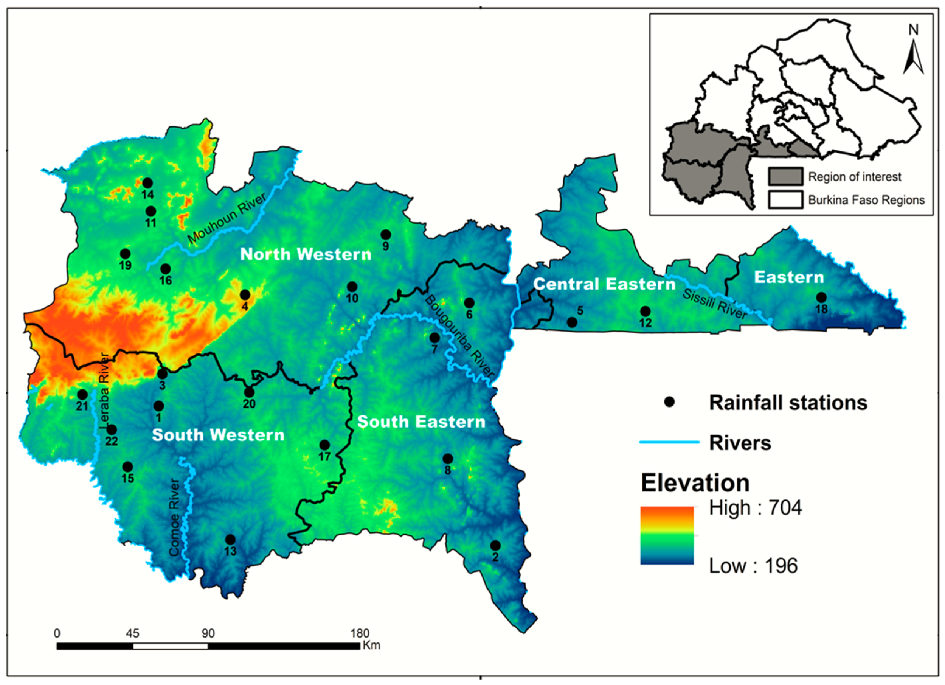
2.1. Study Area

The study area is the southern part of Burkina Faso (Figure 1). The study area has a size of 45,526 km², representing 16,6% of the territory of Burkina Faso. With its tropical climate, the rainy season lasts approximately six months starting in around May–June and ending in around September–October with an annual rainfall ranging between 900 and 1200 mm. It is the rainiest region of Burkina Faso, and its vegetation is dominated by Sudanese savannah. The daily temperature varies between 16 and 45 °C and reaches its highest values in April. The Mouhoun river, also known as the Black Volta river, is the main river of Burkina Faso which allows rural people to develop market gardening activities during the rain-off period.

2.2. Data

We use daily rainfall and sea surface temperature data in this study. The rainfall data for the rainy season, recorded between May and October over 32 years (1986–2017), were collected from the National Meteorological Service (ANAM) of Burkina Faso. Access to in-situ rainfall data was granted by a data request to ANAM. We obtained data from 22 stations, distributed rather equally across our study area (Figure 1).

The West African Sahel rainfall was shown to be positively correlated with the Atlantic SST [20,23], thus being a promising predictor for extreme rainfall in our study area. Atlantic SST data was downloaded from the NOAA National Centers for Environmental Information (NCEI) website (https://www.ncei.noaa.gov/products/avhrr-pathfinder-sst, 13 July 2022). The data is globally available twice a day (day and night) on a grid of 4 km resolution. We use the daily average of SST between May and October over 1986–2017. Since different regions of the Atlantic could have different links with extreme rainfall, we divide the Atlantic area into three equal subregions (North Atlantic, Middle Atlantic, and South Atlantic). The North Atlantic (NA) covers the area between 20° N and 60° N. The Middle Atlantic (MA) comprises the region between 20° N and 20° S, and the region from 20° S to 60°S represents the South Atlantic (SA). We calculated the daily average of SST of all grid values within each subregion and use this average as potential predictors for the frequency and intensity of extreme rainfall.

2.3. Methods

Missing data is one of the major challenges when processing data in climatology and hydrology. About 70% of climate stations obtained from ANAM contained missing data. The percentage of missing data per station ranges between 0.6% and 13.6%. We compare several gap-filling methods [24], namely the Arithmetic Mean (AM), Inverse Distance Weighting (IDW), Normal Ratio (NR), Geographical Coordinates (GC), and Coefficient of Correlation Weighted (CCW) in order to identify the most appropriate one to fill the rainfall data gaps in the study area. Due to a large number of stations, we evaluate the performance of the different methods for one station and use the best-performing method to fill data gaps at all stations with missing data. The Kendall coefficient of correlation ($\tau$) and root mean square error (RMSE) are used to quantify the performance of the candidate methods [25].

Using the gap-filled rainfall time series, we analyze rainfall trends across the study area. To this end, we select 8t rainfall indicators that are part of the 27 indices of rainfall and temperature indicators defined and recommended by the Expert Team on Climate Change Detection and Indices (ETCCDI, [26]). Our set of indices contains three metrics describing the mean behavior of rainfall and five metrics quantifying extreme rainfall (

Table 1. Precipitation indices were used in this study to characterize (extreme) rainfall behavior.

Index	Name	Unit	Description
R1day	Wet days	Days	Annual number of wet days (day with rainfall ≥ 1 mm)
R10	Heavy precipitation days	Days	Annual number of days with rainfall ≥ 10 mm
R20	Very heavy precipitation days	Days	Annual number of days with rainfall ≥ 20 mm
R95p	Very wet days	Days	Annual number of days with rainfall ≥ 95th percentile of the wet days
SDII	Simple daily intensity	mm/day	Mean rainfall on wet days
RX1day	Maximum 1-day precipitation	Mm	Annual maximum 1-day rainfall
RX5day	Maximum 5-day precipitation	Mm	Annual maximum of consecutive 5-days rainfall
PRCPTOT	Total wet-day precipitation	Mm	Annual total from wet days

).

Trends are quantified by Sen’s slope and the Mann–Kendall test with a significance level of 5%. Both methods are non-parametric approaches that are widely used for analyzing gradual trends in climatological and hydrological time series (e.g., [27,28,29,30]). To obtain maps of rainfall trends, station trends are spatially interpolated by means of Inverse Distance Weighting (IDW), which is one of the recommended methods for rainfall interpolation [25,31].

In order to analyze the influence of the Atlantic SST on the frequency and intensity of extreme rainfall, we apply the Peak-Over-Threshold (POT) approach of Extreme Value Theory within a nonstationary framework [32,33,34]. The POT approach is frequently preferred over the Block Maxima approach as it makes better use of extremes [34]. When the threshold u is optimally selected, POT converges toward a Generalized Pareto (GP) distribution:

$$GP\left(z|{\sigma }_u\left(s\right),\gamma \left(s\right)\right)=1-{\left(1-\frac{z\gamma \left(s\right)}{{\sigma }_u\left(s\right)}\right)}_{+}^{-1/\gamma \left(s\right)},$$

(1)

where ${\sigma }_u\left(s\right)$ and $\gamma \left(s\right)\left(\gamma \left(s\right)\ne 0\right)$ are the scale and shape parameters, respectively, at the site $s$ to be estimated and z is a value of rainfall over the threshold u with z > 0. The shape parameter determines the type of distribution. Negative values of $\gamma \left(s\right)$ imply that the distribution GP is bounded, while the distribution GP has no upper bound for $\gamma \left(s\right)>0$. Thus, for positive shape values, the distribution is heavy-tailed [34].

The main challenge of the POT approach is the selection of an optimal threshold that minimizes the bias in the parameter estimation; too high a threshold generates too few excesses leading to high variance, while too low a threshold likely violates the asymptotic basis of the model leading to bias [34]. We use the graphical methods of threshold stability and mean excess plots to select an optimal threshold. These methods consist of finding an appropriate threshold where the plots are approximately linear. Above the threshold, the excesses tend to form clusters, creating a form of dependency amongst elements of the same cluster, while Extreme Value Theory assumes that the data should be independent and identically distributed. A simple way to handle this dependence of exceedances above the threshold is to decluster them by determining clusters of excesses and replacing them with their maximum [35]. The new dataset sampled from the maximum of each cluster is used to estimate the model parameters.

Given an optimal threshold, the excesses over the threshold u converge to the Poisson process with rate parameter $\lambda \left(s\right)$ [33,36,37]. The probability mass function of the Poisson process is given as:

$$PP\left[\lambda \left(s\right)\right]=\frac{exp\left(-\lambda \left(s\right)\right)\lambda {\left(s\right)}^n}{n!},$$

(2)

with n = 1, 2..., N, where $\lambda \left(s\right)>0$ is the rate parameter and N is the number of exceedances of daily rainfall above the threshold u.

The combination of both Poisson and GP distributions is known as the Poisson-GP model, and the probability that the cluster maximum of the Poisson-GP model is less than $z>u$ is expressed as [38]:

$$Pr\left\{ma{x}_{ 1<i<N} Y_{i }\le z\right\}=exp\left\{-\lambda \left(s\right){\left(1+\gamma \left(s\right)\frac{z-u}{{\sigma }_u\left(s\right)}\right)}^{-1/\gamma \left(s\right)}\right\},$$

(3)

where ${\sigma }_u\left(s\right)$ and $\gamma \left(s\right)$ are the scale and shape parameters of the GP model, respectively, and $\lambda \left(s\right)$ is the rate parameter of the Poisson distribution. The Poisson-GP model allows the description of the intensity of extreme rainfall via the GP distribution and the frequency of extreme rainfall via the Poisson distribution.

To quantify the influence of the Atlantic SST on extreme rainfall in the study area, we define SST as a covariate in the nonstationary POT approach. We thus consider the scale and rate parameters as functions depending on the daily average of SST of the Atlantic Ocean. For both dependencies we use an exponential function, ensuring positive values of these parameters [34] for all SST values. As the estimation of the shape parameter is highly uncertain, it is not recommended to express this parameter as a function depending on covariates in a nonstationary framework [34]. The parameters of the nonstationary Poisson-GP model are thus expressed as:

$$\{\begin{array}{c}{\sigma }_u\left(s,T\right)=exp\left({\alpha }_{0,s}+{\alpha }_{1,s}{T}_1+{\alpha }_{2,s}{T}_2+{\alpha }_{3,s}{T}_3 \right)\\ \lambda \left(s,T\right)=exp\left({\beta }_{0,s}+{\beta }_{1,s}{T}_1+{\beta }_{2,s}{T}_2+{\beta }_{3,s}{T}_3\right)\\ \gamma \left(s,T\right)={\gamma }_{0,s}\end{array},$$

(4)

where ${\sigma }_u$, $\gamma$, and $\lambda$ are the scale, shape, and rate parameters, and $T_1$, $T_2$, and $T_3$ denote the average daily SST of the NA, MA, and SA. ${\alpha }_{i,s}$ and ${\beta }_{i,s}$ ($i=0,1,2,3$) are parameters to be estimated for site $s$. The distribution of GP characterized by ${\sigma }_u\left(s,T\right)$ and $\gamma \left(s,T\right)$ is used to analyze the intensity of extreme rainfall, and $\lambda \left(s,T\right)$ characterizes the Poisson distribution for analyzing the frequency of extreme rainfall. The parameters ${\alpha }_{i,s}$ and ${\beta }_{i,s}$ are slopes of ${\sigma }_u\left(s,T\right)$ and $\lambda \left(s,T\right)$, respectively, which allow the evaluation of the change of extreme rainfall intensity and frequency at each station s under the influence of Atlantic SST.

The likelihood ratio test at the 5% significance level is employed to determine which of the two Poisson-GP models (stationary and nonstationary) is preferred given the sample of extreme rainfall. We use the deviance statistic:

$$D=2\left\{l\left(M\right)-l\left(M_0\right)\right\},$$

(5)

where $l\left(M\right)$ and $l\left(M_0\right)$ are the maximized log-likelihood functions of the nonstationary model M and the stationary model M₀, respectively. The deviance statistic D follows a Chi-square distribution of υ degree of freedom, where υ is the difference in the number of the parameters of M and M₀ [34]. The model M₀ is nested within M with the parameters of M₀ being a subset of the parameters of M. In this case, if the p-value of the deviance statistic D is lower than 5%, then the hypothesis that the stationary model M₀ is preferred over the nonstationary model M is rejected. In that case, the nonstationary Poisson-GP model with parameters depending on Atlantic SST better fits the extreme rainfall than the stationary model with constant parameters. Once the choice between the stationary and nonstationary model was conducted based on the deviance test, it is necessary to check whether the adopted model fits the data well. To assess model validity, quantile plots and probability plots are commonly used graphical methods to perform model diagnosis in the univariate framework of extreme value analysis [34]. Considering $z_1\left(s\right)\le z_2\left(s\right)\le \dots$ ≤ $z_n\left(s\right)$ as an ordered sample of the independent observations used to estimate the selected model, then a probability plot consists of the points

$$\left\{\left(\widehat{F}\left(z_i\left(s\right)\right),\frac{i}{1+n}\right),i=1,2,\dots ,n\right\}$$

(6)

and the quantile plot consists of the points

$$\left\{\left(\dot{{\widehat{F}}^{-1}\left(\frac{i}{1+n}\right)},z_i\left(s\right)\right),i=1,2,\dots ,n\right\}$$

(7)

where $\widehat{F}$ and ${\widehat{F}}^{-1}$ are the estimated GP-Poisson model and its inverse function that was selected based on the deviance test (see Equation (5)), respectively. Thus, the model is considered to fit the data well when both the probability plot and quantile plot are close to the unit diagonal [34].

3. Results

3.1. Rainfall Gap Filling

We generate artificial data gaps (5%, 10%, and 15%) at a station with few data gaps, then we use all of the five candidate methods to fill the gaps and calculate $\tau$ and RMSE. The performance of the five candidate methods to fill data gaps is given in

Table 2. Performance of gap-filling methods for station 1 (for location see Figure 1), which has few data gaps, using the Kendall coefficient of correlation ($\tau$) and root mean square error (RMSE).

	5% of Missing Data		10% of Missing Data		15% of Missing Data
	τ	RMSE	τ	RMSE	τ	RMSE
AM	0.46	10.23	0.50	9.71	0.47	9.86
NR	0.46	10.21	0.50	9.73	0.47	9.84
IDW	0.96	2.29	0.92	2.93	0.88	3.71
CC	0.47	9.96	0.49	9.12	0.48	9.71
GC	0.47	10.11	0.47	9.12	0.48	3.91

for three fractions of missing data. IDW shows the best performance; it obtains the highest Kendall coefficient of correlation and the smallest RMSE. Its performance is substantially better than the performance of the other methods. This result agrees with other studies that found IDW to be a suitable method for rainfall data gap filling [24,39]. Hence, we use IDW to fill the data gaps in rainfall time series throughout the study area.

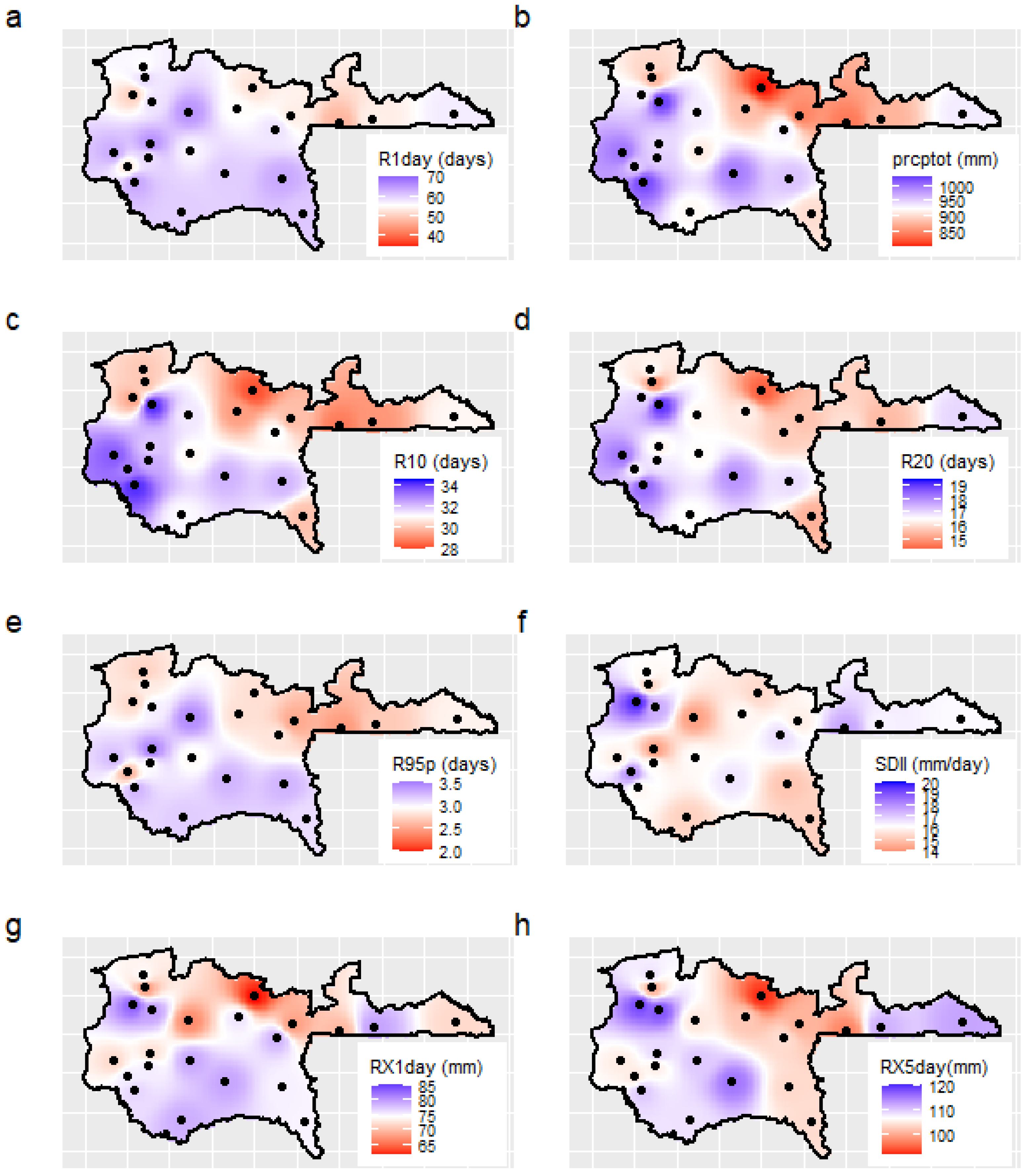
3.2. Preliminary Statistics of Climatology Rainfall

The climatological average of the number of wet days (R1day); the total wet-day precipitation (PRCPTOT); the annual maximum 1-day rainfall (RX1day); and the annual number of days with rainfall ≥10 mm (R10), ≥20 mm (R20) and ≥95th percentile (R95p) show some similarities in terms of distribution (Figure 2a–e,g,h). The higher values of these indices with respect to their average (see Mean,

Table 3. Climatology (normal) precipitation characteristics are given by minimum (Min), average (Mean), standard deviation (SD), and maximum (Max). Min, mean, SD, and max of a given index provide climatological precipitation of the corresponding index at the study area level.

Indices	Min	Mean (±SD)	$\mathbf{Max}$
R1day	48	58.2 ± 4.8	66
PRCPTOT	803.7	927.5 ± 57.6	1029.8
R10	28.3	31.1 ± 1.6	34.1
R20	14.3	16.6 ± 1.2	19.1
R95p	2.5	3.0 ± 0.3	3.5
SDII	14.4	16.2 ± 1.2	19.6
RX1day	61.8	74.5 ± 5.1	83.0
RX5day	92.8	106.7 ± 6.2	118.2

) are observed in the southwest part of the study area, while the eastern part has recorded values relatively lower than their average. The climatological distribution of annual maximum precipitation over five consecutive days (RX5days) differs from the distribution of previous rainfall indices. The higher values of RX5days with respect to its average are observed in the western and eastern parts, whereas its lower values are mostly found in the central part of the study area. As for SDII (mean rainfall on wet days), it is almost uniformly distributed over the study area (Figure 2f) with values more or less close to the average of 16.2 mm/day. Except for SDII and RX5day rainfall indices, most of the stations with rainfall index values lower than their average are in the northern part of the study area, implying that the rainfall indices have decreased climatologically from northeast to westsouth over the study area.

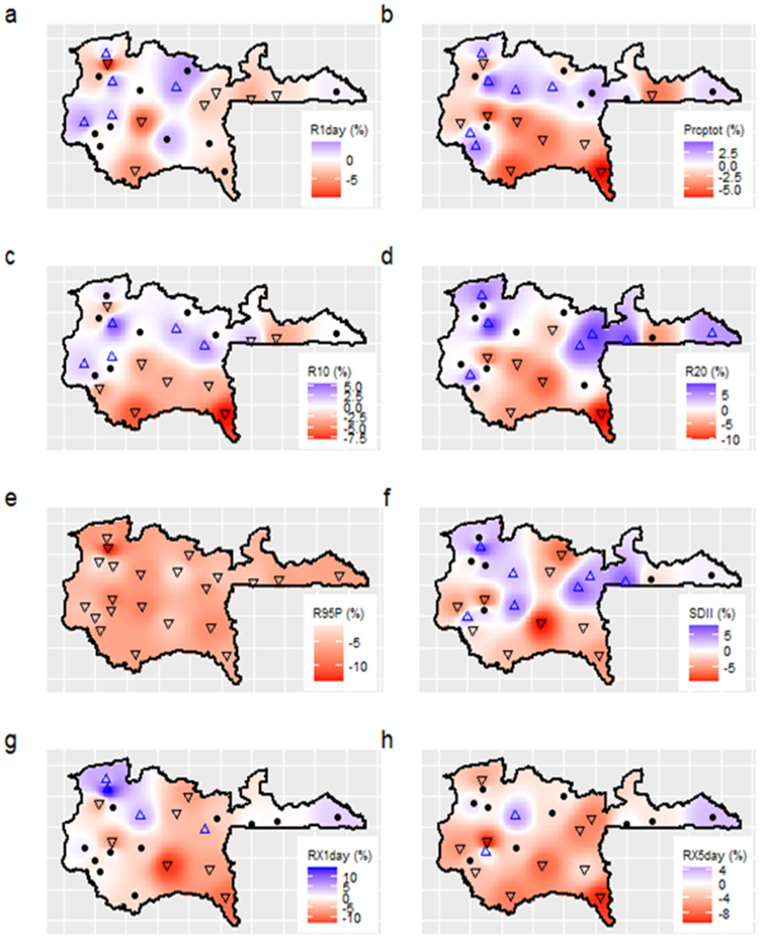
3.3. Rainfall Trends

Changes in the number of wet days (R1day) show increases and decreases between −9.9% and 4.4% per decade (Figure 3a). The three eastern regions show only decreasing trends (some of them not significant), while the two western zones show a mixture of upward and downward changes. For total wet-day precipitation (PRCPTOT) we also detect a mixture of changes (Figure 3b) with 27% (41%) of stations showing significant upward (downward) trends. The spatial pattern of changes shows a tendency towards decreasing (increasing) precipitation in the southern (northern) parts. Trends at single stations range from−6.8% to 4.6% per decade. Overall, we find different patterns for changes in R1day and PRCPTOT, and the direction of change in total precipitation is not at all stations aligned with the direction of change in the number of wet days. The effect of the superposition of both indicators is seen in SDII (mean rainfall on wet days, Figure 3f). Mean daily rainfall intensity has changed significantly at 73% of stations with values between −9.6% and 7.6% per decade. There is a tendency towards decreases in the south, while the north shows a mixture of areas with increasing and decreasing trends.

The spatial patterns for the annual maximum 1-day rainfall (RX1day) and annual maximum of consecutive 5-days rainfall (RX5days) show some similarities (Figure 3g,h). The south (southwestern and southeastern) tends to show downward trends, while the western part of the northwestern region shows upward trends (up to 14.2% per decade) or nonsignificant changes. Overall, we detect a tendency towards less intensive 1-day and 5-day rainfall maxima. Relatively to the frequency indices of heavy rainfall, i.e., the annual number of days with rainfall ≥10 mm (R10), ≥20 mm (R20) and ≥95th percentile of the wet days (R95p), respectively, we find mostly downward trends (Figure 3c–f). All climate stations show significant downward trends for R95P with values between −13.5% and −1.6% per decade. The spatial patterns for R10 and R20 are less homogeneous with some areas in the northern part with significant upward trends.

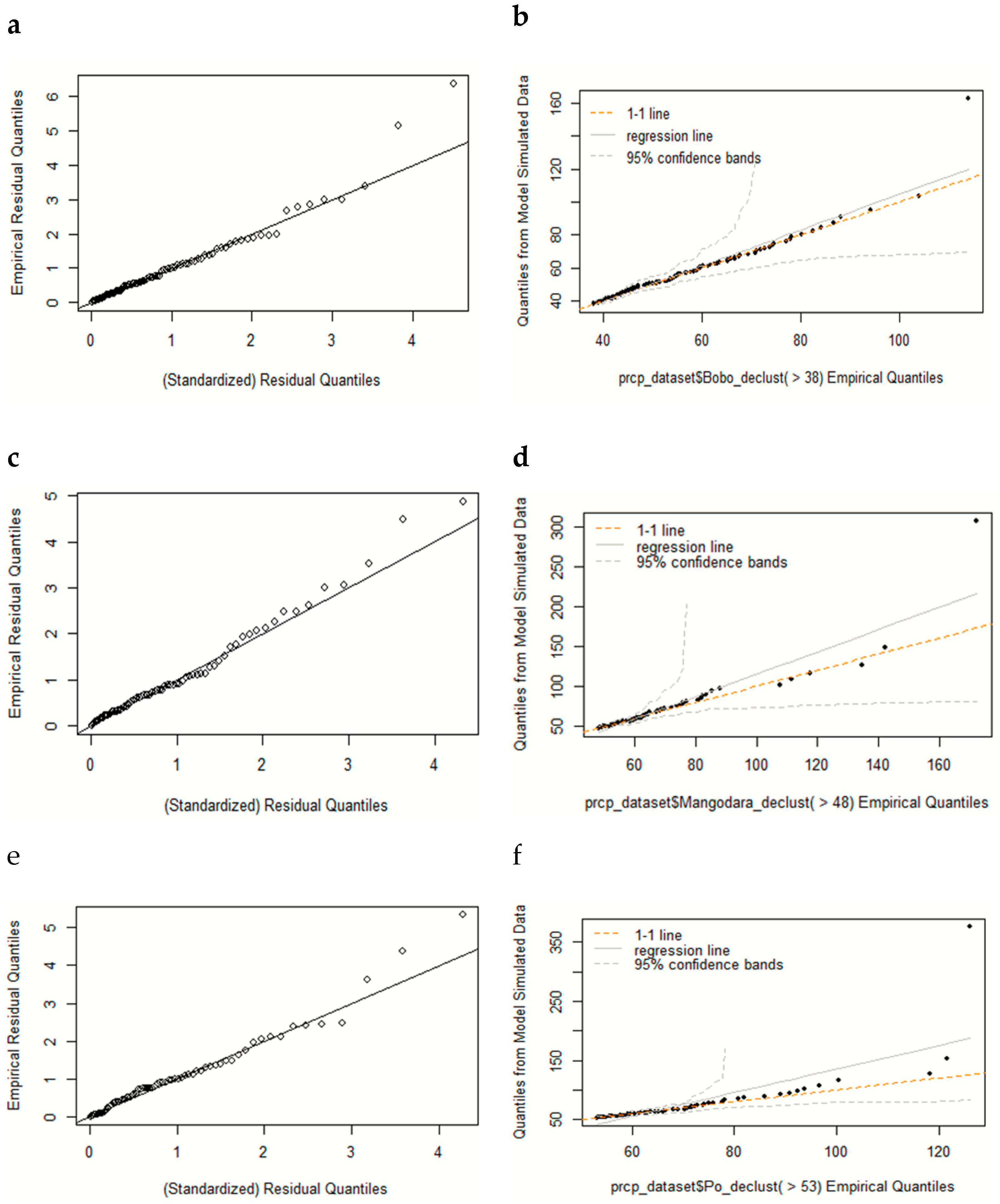
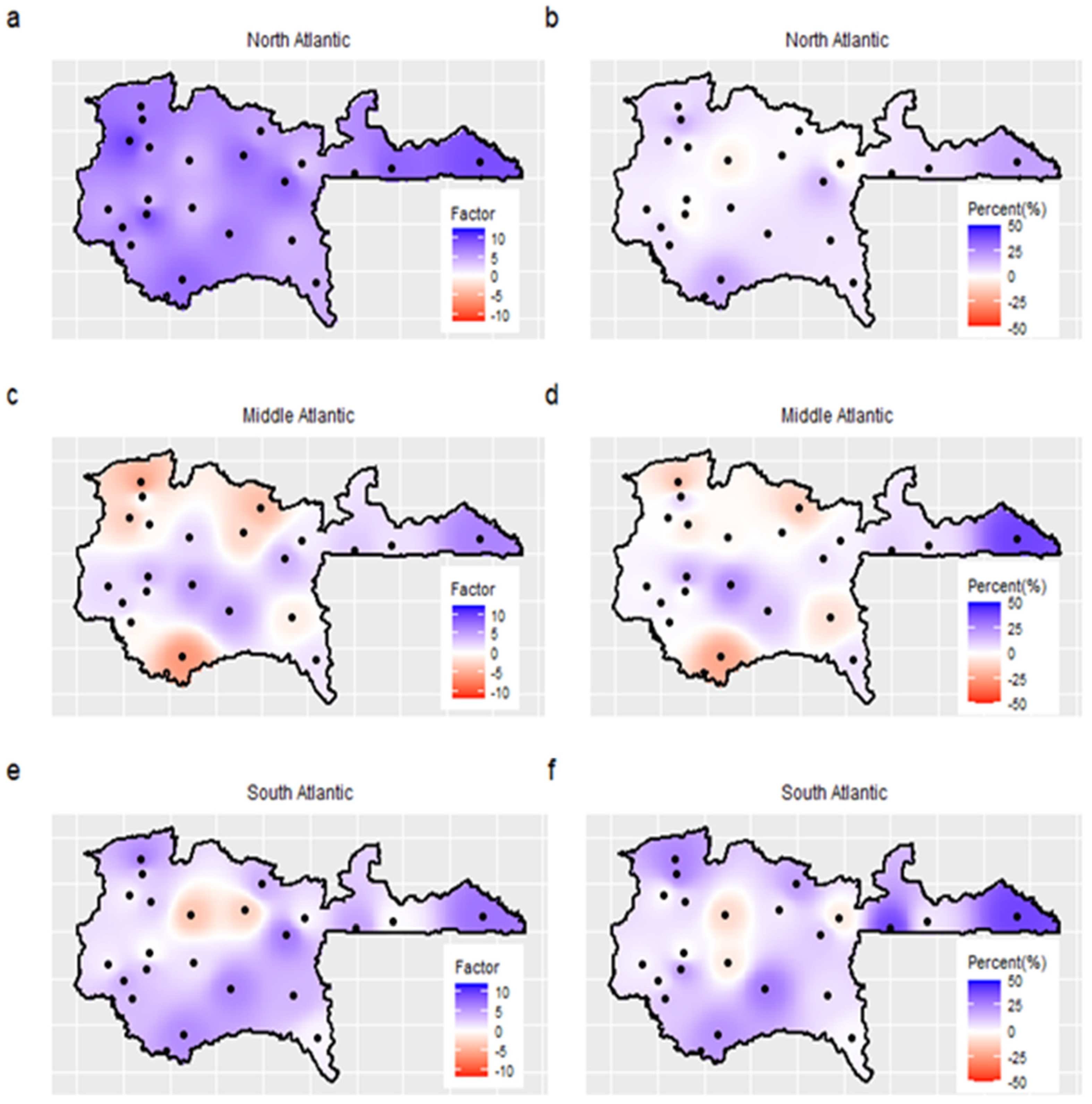
3.4. Link between Atlantic SST and Heavy Rainfall

Using the threshold stability and mean excess graphical methods, we select an optimal threshold beyond which daily rainfall is considered extreme rainfall. The optimal threshold to ensure the stability of Poisson-GP parameters ranges from 30 to 53 mm with an average value of 41.6 mm across all stations. With these thresholds, an average of 2.4% of daily rainfall is considered extreme rainfall with a range from 1.1% to 4.5%. After the threshold selection and the decluttering of excess values, we fit the stationary and the nonstationary Poisson-GP models using the maximum likelihood method. Based on the deviance statistic we find that the nonstationary Poisson-GP model with parameters depending on the daily SST of NA, MA, and SA is preferred over the stationary model to represent the extreme rainfall at all stations. Table 3 shows the deviance and the p-value associated with the deviance test for each station (see Figure 1 for station locations). At the 5% significance level, the deviance test at all stations is statistically significant, meaning that the non-stationary model SST as a covariable outperforms the stationary model (see Table 3).

Table 4. Performance of the deviance test at a 5% significance level for all the climate stations using the p-values associated with deviance value (see Figure 1 for station localization).

Station	1	2	3	4	5
Deviance	85.07	148.58	42.76	60.49	38.99
p-value	$3.19\times {10}^{-16}$	$2.20\times {10}^{-16}$	$1.30\times {10}^{-7}$	$3.58\times {10}^{-11}$	$7.18\times {10}^{-7}$
Station	6	7	8	9	10
Deviance	27.61	48.54	33.08	42.45	45.20
p-value	$1.11\times {10}^{-4}$	$9.03\times {10}^{-9}$	$1.01\times {10}^{-5}$	$1.50\times {10}^{-7}$	$4.28\times {10}^{-8}$
Station	11	12	13	14	15
Deviance	60.56	45.39	40.16	69.31	36.51
p-value	$3.47\times {10}^{-11}$	$3.92\times {10}^{-8}$	$4.24\times {10}^{-7}$	$5.66\times {10}^{-13}$	$2.20\times {10}^{-6}$
Station	16	17	18	19	20
Deviance	83.93	49.67	51.28	65.77	19.34
p-value	$5.51\times {10}^{-16}$	$5.47\times {10}^{-9}$	$2.60\times {10}^{-9}$	$3.00\times {10}^{-12}$	$3.63\times {10}^{-4}$
Station	21	22
Deviance	56.20	52.93
p-value	$2.66\times {10}^{-10}$	$1.22\times {10}^{-9}$

shows that the nonstationary models with SST as covariables significantly outperform the stationary models for all the stations. Thus, the validation of the nonstationary model at the station level was performedusing probability and quantile plot methods. The results pointed out that the nonstationary models are well-fitted to the rainfall data. Figure 4 shows the quantile and probability plot results for stations 4, 13 and 18. We found that the quantile and probability plots of these models are close to the unit diagonal. The left column is the quantile plots, and the right column denotes the model probability plots.

Figure 5 shows maps of the slope values (${\alpha }_{1,s},{\alpha }_{2,s},{\alpha }_{3,s},{\mathsf{\beta }}_{1,\mathrm{s}},{\mathsf{\beta }}_{2,\mathrm{s}},and{\mathsf{\beta }}_{3,\mathrm{s}}$; Equation (4)) of the nonstationary models. The frequency of extreme rainfall is positively associated with NA SST throughout the study area with comparatively high slope values in the range of 3.1–9.5 (Figure 5a). That means that the frequency of extreme rainfall increases by a factor of 3 to 9 when SST of NA increases by one degree Celsius. The influence of MA and SA SST varies in the study area (Figure 5c,e); extreme rainfall frequency is positively affected by higher SST values in some areas, while other areas are negatively affected. The slope values of MA and SA are somewhat lower compared to the slope values slopes of NA. The average of the absolute slopes is 6, 0.6, and 2.6 for NA, MA, and SA, respectively. Hence, changes in SST of NA tend to have a stronger effect compared to changes in SST in MA and SA. For the eastern region we find large positive associations between the frequency of extreme rainfall and SST in all three parts of the Atlantic.

The intensity of extreme rainfall is significantly linked to the SST of NA, MA, and SA, but the sign of this correlation is not homogeneous over the study area (Figure 5b,d,f). SST of NA is positively associated with the intensity of heavy rainfall for most stations. The slope values vary between 3.9% and 20.1% per °C. SST of MA only locally influences the intensity of extreme rainfall in rather small areas in the central, southern, and eastern parts. SA SST tends to increase extreme precipitation in the north and south, and decrease extreme precipitation in central parts. For the Eastern region, we find a strong positive association for all three parts of the Atlantic Ocean. Here, we find the highest slope values. The intensity of extreme precipitation increases by 20.1%, 40.1%, and 39.9% per °C increase in SST of NA, MA, and SA, respectively.

4. Discussion

To inform disaster risk reduction and climate adaptation at the local scale in West Africa, it is important to understand the space-time behavior of rainfall. Understanding of space–time variation in precipitation is necessary for the identification and monitoring of flash flood hotspots, which facilitates the appropriate allocation of resources to flood risk projects for a more effective emergency response to floods. Our study shows that rainfall trends are spatially heterogeneous in southern Burkina Faso. Large-scale trend studies at the national or supranational scale have concluded that extreme rainfall has become more frequent and intense in West Africa [5,10,11,12]. We find not only a much more nuanced behavior, based on the much higher density of stations in our study, but also some opposite effects. For most rainfall indices, we find decreasing trends at the majority of stations. Similar results were found by other local studies in the Oti Bassin in Togo [40] and in the Vea catchment in Ghana, where more than 78% of stations showed downward trends in the intensity and frequency of extreme rainfall [41]. This discrepancy between the large-scale studies and local studies suggests that national or supranational studies may misinterpret rainfall trends when they are based on scarce data.

Besides the overall tendency towards decreasing trends, we also find areas with increasing trends. Most stations with upward trends are located in the northern part of our study area. As this part is drier than the southern part, the standard catchphrase ‘dry gets drier, wet gets wetter’ does not hold in our study area. It needs to be mentioned, however, that the evidence for this catchphrase is rather weak [42].

Our nonstationary Poisson-GP model suggests that the frequency and intensity of extreme rainfall are linked to SST in the Atlantic Ocean. The northern part of the Atlantic plays a larger role, in particular in the frequency of extreme rainfall. Given the observed and expected warming of the Atlantic as a consequence of anthropogenic climate change [43], our modeling approach suggests that the hypothesis of stationary is no longer suitable for extreme rainfall analysis in the study area.

The impact of the Atlantic SST on the frequency and intensity of extreme rainfall was estimated at the station level and spatially interpolated using the inverse distance weighted method. This approach has the advantage of simplicity but does not consider the spatial dependence structure. An alternative, more sophisticated approach would be the generalized pareto process modeling [44] which is able to capture the spatial correlation directly in the modeling framework. Further, we considered only the SST of the Atlantic. A more comprehensive analysis including SST of other regions and/or other atmospheric variables could result in more skillful covariates in the statistical modeling of extreme rainfall.

Our trend results, i.e., more downward trends than upward trends, seem to contradict the general evolution of increasing flood events in Burkina Faso and adjacent countries. We cannot attribute the increasing number of flood events and affected people to increasing rainfall extremes. Only in the northwestern part of our study area, did we find increasing trends, particularly in RX1day. This area is the second most frequently flooded region in Burkina Faso from 1986 to 2016, affecting many people and their properties, only surpassed by the central region of Burkina Faso [3]. Upward trends in extreme rainfall may have contributed to this flood hotspot. This is in line with a study conducted in Mali by [45] who found that flash floods are extremely related to extreme rainfall. Otherwise, our analysis supports the explanation that has been concluded for the increasing flood risk in Ouagadougou north of our study area; namely that land use and land cover changes, and population and urban growth, accompanied by low investments in flood-resilient infrastructure and management, have been the main drivers of flood risk [3,46]. Similar results were found in Mali, the country that borders the study area, where [45] pointed out that about 58% of floods occurrence were caused by normal rainfall. According to the same authors, these floods could be due to changes in land use and land cover and the increase in impervious areas.

5. Conclusions

The study has investigated the spatiotemporal variability of rainfall characteristics and the impact of SST of different areas of the Atlantic Ocean upon the frequency and intensity of extreme rainfall for the period of 1986–2017 in the southern part of Burkina Faso. In contrast to large-scale, data-scarce trend studies that concluded that extreme rainfall has become more frequent and intense in West Africa, our results show a more nuanced picture. Although trends vary with rainfall characteristics and in space, we find more downward trends across the study area, particularly for indices representing extreme rainfall. We also show that a nonstationary Poisson-GP model with SSTs as covariables outperform the stationary Poisson-GP model, which implies that the assumption of a stationary nature has to be considered with care when modeling the frequency and intensity of extreme rainfall. Future work should explore whether the linkage between Atlantic SST variations and extreme rainfall are strong enough to be used in water resources management, for instance, for seasonal rainfall forecasting. Our results suggest that the recent increase in flood disasters is more attributed to land use and land cover changes, and population and urbanization growth than to the increase in rainfall extremes in the southern part of Burkina Faso.

References

1. Salack, S.; Saley, I.A.; Lawson, N.Z.; Zabré, I.; Daku, E.K. Scales for Rating Heavy Rainfall Events in the West African Sahel. Weather Clim. Extrem. 2018, 21, 36–42. [Google Scholar] [CrossRef]
2. Sultan, B.; Gaetani, M. Agriculture in West Africa in the Twenty-First Century: Climate Change and Impacts Scenarios, and Potential for Adaptation. Front. Plant Sci. 2016, 7, 1262. [Google Scholar] [CrossRef] [PubMed] [Green Version]
3. Tazen, F.; Diarra, A.; Kabore, R.F.; Ibrahim, B.; Bologo/Traoré, M.; Traoré, K.; Karambiri, H. Trends in Flood Events and Their Relationship to Extreme Rainfall in an Urban Area of Sahelian West Africa: The Case Study of Ouagadougou, Burkina Faso. J. Flood Risk Manag. 2019, 12, e12507. [Google Scholar] [CrossRef] [Green Version]
4. West Africa—Flood Affected Population—June to September 2009 (as of 14 Oct 2009)—Mauritania | ReliefWeb. Available online: https://reliefweb.int/map/mauritania/west-africa-flood-affected-population-june-september-2009-14-oct-2009 (accessed on 12 August 2022).
5. Panthou, G.; Vischel, T.; Lebel, T. Recent Trends in the Regime of Extreme Rainfall in the Central Sahel. Int. J. Climatol. 2014, 34, 3998–4006. [Google Scholar] [CrossRef]
6. Données Sur Les InondationsàLa Date Du 17 Août 2016—Burkina Faso | ReliefWeb. Available online: https://reliefweb.int/report/burkina-faso/donn-es-sur-les-inondations-la-date-du-17-ao-t-2016 (accessed on 12 August 2022).
7. Olanrewaju, C.C.; Olanrewaju, O.A.; Chitakira, M. Impacts of Flood Disasters in Nigeria: A Critical Evaluation of Health Implications and Management. Jàmbá J. Disaster Risk Stud. 2019, 11, 1–9. [Google Scholar]
8. Alfieri, L.; Bisselink, B.; Dottori, F.; Naumann, G.; de Roo, A.; Salamon, P.; Wyser, K.; Feyen, L. Global Projections of River Flood Risk in a Warmer World. Earth’s Future 2017, 5, 171–182. [Google Scholar] [CrossRef]
9. Merz, B.; Blöschl, G.; Vorogushyn, S.; Dottori, F.; Aerts, J.C.; Bates, P.; Bertola, M.; Kemter, M.; Kreibich, H.; Lall, U. Causes, Impacts and Patterns of Disastrous River Floods. Nat. Rev. Earth Environ. 2021, 2, 592–609. [Google Scholar]
10. Ly Mouhamed; Traore, S.B.; Alhassane, A.; Sarr, B. Evolution of Some Observed Climate Extremes in the West African Sahel. Weather Clim. Extrem. 2013, 1, 19–25. [Google Scholar] [CrossRef] [Green Version]
11. Sanogo, S.; Fink, A.H.; Omotosho, J.A.; Ba, A.; Redl, R.; Ermert, V. Spatio-Temporal Characteristics of the Recent Rainfall Recovery in West Africa. Int. J. Climatol. 2015, 35, 4589–4605. [Google Scholar] [CrossRef]
12. Ta, S.; Kouadio, K.Y.; Ali, K.E.; Toualy, E.; Aman, A.; Yoroba, F. West Africa Extreme Rainfall Events and Large-Scale Ocean Surface and Atmospheric Conditions in the Tropical Atlantic. Adv. Meteorol. 2016, 2016, 1940456. [Google Scholar] [CrossRef] [Green Version]
13. Liu, D.; Li, Y. Social Vulnerability of Rural Households to Flood Hazards in Western Mountainous Regions of Henan Province, China. Nat. Hazards Earth Syst. Sci. 2016, 16, 1123–1134. [Google Scholar] [CrossRef] [Green Version]
14. Dai, A.; Wigley, T.M.L. Global Patterns of ENSO-Induced Precipitation. Geophys. Res. Lett. 2000, 27, 1283–1286. [Google Scholar] [CrossRef]
15. Conticello, F.; Cioffi, F.; Merz, B.; Lall, U. An Event Synchronization Method to Link Heavy Rainfall Events and Large-Scale Atmospheric Circulation Features. Int. J. Climatol. 2018, 38, 1421–1437. [Google Scholar] [CrossRef]
16. Gerlitz, L.; Vorogushyn, S.; Apel, H.; Gafurov, A.; Unger-Shayesteh, K.; Merz, B. A Statistically Based Seasonal Precipitation Forecast Model with Automatic Predictor Selection and Its Application to Central and South Asia. Hydrol. Earth Syst. Sci. 2016, 20, 4605–4623. [Google Scholar] [CrossRef] [Green Version]
17. Steinschneider, S.; Lall, U. A Hierarchical B Ayesian Regional Model for Nonstationary Precipitation Extremes in N Orthern C Alifornia Conditioned on Tropical Moisture Exports. Water Resour. Res. 2015, 51, 1472–1492. [Google Scholar] [CrossRef]
18. Sun, X.; Thyer, M.; Renard, B.; Lang, M. A General Regional Frequency Analysis Framework for Quantifying Local-Scale Climate Effects: A Case Study of ENSO Effects on Southeast Queensland Rainfall. J. Hydrol. 2014, 512, 53–68. [Google Scholar] [CrossRef] [Green Version]
19. White, C.J.; Carlsen, H.; Robertson, A.W.; Klein, R.J.T.; Lazo, J.K.; Kumar, A.; Vitart, F.; Coughlan de Perez, E.; Ray, A.J.; Murray, V.; et al. Potential Applications of Subseasonal-to-Seasonal (S2S) Predictions: Potential Applications of Subseasonal-to-Seasonal (S2S) Predictions. Meteorol. Appl. 2017, 24, 315–325. [Google Scholar] [CrossRef] [Green Version]
20. Atiah, W.A.; Mengistu Tsidu, G.; Amekudzi, L.K.; Yorke, C. Trends and Interannual Variability of Extreme Rainfall Indices over Ghana, West Africa. Appl. Clim. 2020, 140, 1393–1407. [Google Scholar] [CrossRef]
21. Diatta, S.; Diedhiou, C.W.; Dione, D.M.; Sambou, S. Spatial Variation and Trend of Extreme Precipitation in West Africa and Teleconnections with Remote Indices. Atmosphere 2020, 11, 999. [Google Scholar] [CrossRef]
22. Nana, T.J. Impact of Climate Change on Cereal Production in Burkina Faso. J. Agric. Environ. Sci. 2019, 8, 14–24. [Google Scholar] [CrossRef]
23. Dieppois, B.; Durand, A.; Fournier, M.; Diedhiou, A.; Fontaine, B.; Massei, N.; Nouaceur, Z.; Sebag, D. Low-Frequency Variability and Zonal Contrast in Sahel Rainfall and Atlantic Sea Surface Temperature Teleconnections during the Last Century. Theor. Appl. Climatol. 2015, 121, 139–155. [Google Scholar] [CrossRef]
24. Suhaila, J.; Sayang, M.D.; Jemain, A.A. Revised Spatial Weighting Methods for Estimation of Missing Rainfall Data. Asia-Pac. J. Atmos. Sci. 2008, 44, 93–104. [Google Scholar]
25. Chen, F.-W.; Liu, C.-W. Estimation of the Spatial Rainfall Distribution Using Inverse Distance Weighting (IDW) in the Middle of Taiwan. Paddy Water Environ. 2012, 10, 209–222. [Google Scholar] [CrossRef]
26. Sillmann, J.; Kharin, V.V.; Zhang, X.; Zwiers, F.W.; Bronaugh, D. Climate Extremes Indices in the CMIP5 Multimodel Ensemble: Part 1. Model Evaluation in the Present Climate. J. Geophys. Res. Atmos. 2013, 118, 1716–1733. [Google Scholar] [CrossRef]
27. Hirsch, R.M.; Slack, J.R. A Nonparametric Trend Test for Seasonal Data with Serial Dependence. Water Resour. Res. 1984, 20, 727–732. [Google Scholar] [CrossRef] [Green Version]
28. Yue, S.; Pilon, P. A Comparison of the Power of the t Test, Mann-Kendall and Bootstrap Tests for Trend Detection/Une Comparaison de La Puissance Des Tests t de Student, de Mann-Kendall et Du Bootstrap Pour La Détection de Tendance. Hydrol. Sci. J. 2004, 49, 21–37. [Google Scholar] [CrossRef]
29. Blöschl, G.; Hall, J.; Viglione, A.; Perdigão, R.A.; Parajka, J.; Merz, B.; Lun, D.; Arheimer, B.; Aronica, G.T.; Bilibashi, A. Changing Climate Both Increases and Decreases European River Floods. Nature 2019, 573, 108–111. [Google Scholar] [CrossRef]
30. Sa’adi, Z.; Shahid, S.; Ismail, T.; Chung, E.-S.; Wang, X.-J. Trends Analysis of Rainfall and Rainfall Extremes in Sarawak, Malaysia Using Modified Mann–Kendall Test. Meteorol. Atmos. Phys. 2019, 131, 263–277. [Google Scholar] [CrossRef]
31. Yang, X.; Xie, X.; Liu, D.L.; Ji, F.; Wang, L. Spatial Interpolation of Daily Rainfall Data for Local Climate Impact Assessment over Greater Sydney Region. Adv. Meteorol. 2015, 2015, 563629. [Google Scholar] [CrossRef] [Green Version]
32. Acero, F.J.; García, J.A.; Gallego, M.C. Peaks-over-Threshold Study of Trends in Extreme Rainfall over the Iberian Peninsula. J. Clim. 2011, 24, 1089–1105. [Google Scholar] [CrossRef]
33. Acero, F.J.; García, J.A.; Gallego, M.C.; Parey, S.; Dacunha-Castelle, D. Trends in Summer Extreme Temperatures over the Iberian Peninsula Using Nonurban Station Data. J. Geophys. Res. Atmos. 2014, 119, 39–53. [Google Scholar] [CrossRef]
34. Coles, S. An Introduction to Statistical Model of Extremes Values, 1st ed.; Springer Series in Statistics; Springer-Verlag: London, UK, 2001; ISBN 978-1-84996-874-4. [Google Scholar]
35. Gilleland, E.; Katz, R.W. ExtRemes 2.0: An Extreme Value Analysis Package in R. J. Stat. Softw. 2016, 72, 1–39. [Google Scholar] [CrossRef] [Green Version]
36. Hamdi, Y.; Charron, C.; Ouarda, T.B. A Non-Stationary Heat Spell Frequency, Intensity, and Duration Model for France, Integrating Teleconnection Patterns and Climate Change. Atmosphere 2021, 12, 1387. [Google Scholar] [CrossRef]
37. Tramblay, Y.; Neppel, L.; Carreau, J.; Najib, K. Non-Stationary Frequency Analysis of Heavy Rainfall Events in Southern France. Hydrol. Sci. J. 2013, 58, 280–294. [Google Scholar] [CrossRef]
38. Smith, R. Statistics of Extremes, with Applications in Environment, Insurance and Finance; CRC Press: Boca Raton, FL, USA, 2002; Volume 99. [Google Scholar] [CrossRef]
39. Ismail, W.W.; Zin, W.Z.W.; Ibrahim, W. Estimation of Rainfall and Stream Flow Missing Data for Terengganu, Malaysia by Using Interpolation Technique Methods. Malays. J. Fundam. Appl. Sci 2017, 13, 214–218. [Google Scholar] [CrossRef]
40. Klassou, K.S.; Komi, K. Analysis of Extreme Rainfall in Oti River Basin (West Africa). J. Water Clim. Chang. 2021, 12, 1997–2009. [Google Scholar] [CrossRef]
41. Larbi, I.; Hountondji, F.C.; Annor, T.; Agyare, W.A.; Mwangi Gathenya, J.; Amuzu, J. Spatio-Temporal Trend Analysis of Rainfall and Temperature Extremes in the Vea Catchment, Ghana. Climate 2018, 6, 87. [Google Scholar] [CrossRef] [Green Version]
42. Greve, P.; Orlowsky, B.; Mueller, B.; Sheffield, J.; Reichstein, M.; Seneviratne, S.I. Global Assessment of Trends in Wetting and Drying over Land. Nat. Geosci. 2014, 7, 716–721. [Google Scholar] [CrossRef]
43. Masson-Delmotte, V.; Zhai, P.; Pirani, A.; Connors, S.L.; Péan, C.; Berger, S.; Caud, N.; Chen, Y.; Goldfarb, L.; Gomis, M.I. Climate Change 2021: The Physical Science Basis. Contrib. Work. Group I Sixth Assess. Rep. Intergov. Panel Clim. Chang. 2021, 2. [Google Scholar]
44. Palacios-Rodríguez, F.; Toulemonde, G.; Carreau, J.; Opitz, T. Generalized Pareto Processes for Simulating Space-Time Extreme Events: An Application to Precipitation Reanalyses. Stoch. Environ. Res. Risk Assess. 2020, 34, 2033–2052. [Google Scholar] [CrossRef]
45. Fofana, M.; Adounkpe, J.; Larbi, I.; Hounkpe, J.; Koubodana, H.D.; Toure, A.; Bokar, H.; Dotse, S.-Q.; Limantol, A.M. Urban Flash Flood and Extreme Rainfall Events Trend Analysis in Bamako, Mali. Environ. Chall. 2022, 6, 100449. [Google Scholar] [CrossRef]
46. Aich, V.; Liersch, S.; Vetter, T.; Andersson, J.C.; Müller, E.N.; Hattermann, F.F. Climate or Land Use?—Attribution of Changes in River Flooding in the Sahel Zone. Water 2015, 7, 2796–2820. [Google Scholar] [CrossRef]
Figure 1. Topography, main rivers, and rainfall stations of the study area are located in the southern part of Burkina Faso. Eastern, central eastern, northwestern, southeastern and southwestern are administrative areas of Burkina Faso corresponding to Nahouri, Sissili, Haut-Bassins, Sud-Ouest, and Cascades.
Atmosphere 14 00284 g001
Figure 2. Distribution rainfall indices given as the climatological average of R1day (a), PRCPTOT (b), R10 (c), R20 (d), R95p (e), SDII (f), RX1day (g), and RX5day (h) distributed over the study area. Circles denote climate stations. The blue (respectively red color) represents the areas with the index value higher (respectively lower) than the climatological average of the study area and the white color corresponds to the value close to the climatological average of rainfall indices. Maps are obtained by interpolating station values using the IDW method.
Atmosphere 14 00284 g002
Figure 3. Trends in rainfall indices given as change per decade in % for R1day (a), PRCPTOT (b), R10 (c), R20 (d), R95p (e), SDII (f), RX1day (g), and RX5days (h). Upward/downward triangles denote stations with statistically significant upward/downward trends at the 5% significance level. Circles show stations with non-significant changes. Maps are obtained by interpolating station values using the IDW method.
Atmosphere 14 00284 g003
Figure 4. Quantile (a,c,e) and probability (b,d,f) plots of the nonstationary GP-Poisson model for stations 4, 13 and 18, respectively. These are located in the northwest, southwestern and eastern (see, Figure 1) areas, respectively. The left column denotes the quantile plots (a,c,e) of the nonstationary models for station 4, 13 and 18, respectively. The right column represents the probability plots (b,d,f) of the same models estimated at stations 4, 13 and 18. The quantile plots (a,c,e respectively) and the probability plots (b,d,f) of the nonstationary models for station 4, 13 and 18 respectively, are close to unit diagonal which implies that the nonstationary models fit well the data.
Atmosphere 14 00284 g004
Figure 5. Slope values of the linear relations between SST and extreme rainfall. Left column: Slope values ( β 1 , s ,   β 2 , s ,   a n d   β 3 , s ) for the frequency of extreme rainfall. A value of n means an n-fold increase in the frequency of extreme precipitation per °C increase in SST. Right column: Slope values ( α 1 , s , α 2 , s , and α 3 , s ) for the intensity of extreme rainfall. A value of n means an n% increase in the intensity of extreme precipitation per °C increase in SST. Rows represent the different covariates, i.e., SST of North Atlantic (upper), SST of Middle Atlantic (middle), and SST of South Atlantic (lower). The impact of Atlantic SST on extreme rainfall is estimated at the station level and interpolated spatially using the IDW method. The circles are rainfall stations. Figures (a,c,e) express the influence of upper, middle, and lower Atlantic SSTs, respectively, on the frequency of extreme rainfall. Figures (b,d,f) represent the influence of upper, middle, and lower Atlantic SSTs, respectively, on the intensity of extreme rainfall.
Atmosphere 14 00284 g005