Article

Diurnal Variation Characteristics of the Surface Sensible Heat Flux over the Tibetan Plateau

1
Key Laboratory of Meteorological Disaster, Ministry of Education (KLME)/Collaborative Innovation Center on Forecast and Evaluation of Meteorological Disasters (CIC-FEMD)/Joint International Research Laboratory of Climate and Environment Change (ILCEC)/Joint Center for Data Assimilation Research and Applications, School of Atmospheric Sciences, Nanjing University of Information Science & Technology, Nanjing 210044, China
2
International Institute for Earth System Science, Nanjing University, Nanjing 210033, China
3
China Meteorological Administration Training Center, Beijing 100081, China
*
Authors to whom correspondence should be addressed.
Atmosphere 2023, 14(1), 128; https://doi.org/10.3390/atmos14010128
Submission received: 1 November 2022 / Revised: 26 December 2022 / Accepted: 3 January 2023 / Published: 6 January 2023

Abstract

:
The characteristics of diurnal variation of the surface sensible heat flux (SH) over the Tibetan Plateau (TP) are comprehensively investigated by using the long-term dataset of integrated land–atmosphere interaction observations (2006–2016) on the TP. Results show that the diurnal variation of SH shows obvious seasonal variabilities in terms of amplitude, duration, and peak time. At the Muztagh Ata Westerly Observation and Research Station (MAWORS), the Ngari Desert Observation and Research Station (NADORS), and the Qomolangma Atmospheric and Environmental Observation and Research Station (QOMS), the SH diurnal amplitude is consistently the largest in spring, followed by summer and autumn, and the smallest in winter, with a peak at 15:00. However, for the Southeast Tibet Observation and Research Station (SETORS), the amplitude in winter is rather violent with the peak at 12:00. We find that positive SH at most stations has the longest duration from May to August. Moreover, the peak time fluctuates from month to month, even showing a shift at the QOMS before and after 2015, and the double-peak phenomenon of SH mainly occurs in spring and autumn. Additionally, magnitudes of calculated SH with the conventional heat transfer coefficient (CDH) of 0.004 are about 64% to 100% larger than those of directly observed SH at the QOMS and the Nam Co Monitoring and Research Station (NAMORS). We here additionally recommend a new CDH values of about 2.24 × 10⁻³ in spring and 2.78 × 10⁻³ in summer, respectively, to more accurately calculate the TP SH.

1. Introduction

The Tibetan Plateau (TP) occupies about a quarter of the land area of China, with an average elevation of more than 4000 m. It is well known as “the roof of the world” and “the third pole of the Earth” [1]. Surface sensible heat flux (SH), as one of the significant parameters to characterize the strength of the interaction between surface and atmosphere, accelerates the updraft in spring and summer, which can directly act on the middle troposphere and modulate the atmospheric circulations to affect the Asian summer monsoon variabilities [2,3,4,5] and even the development of tropical ENSO and the air–sea interaction in the mid-latitude Pacific [6]. Duan et al. [7] have pointed out that the SH from April to June over the TP can be used as an effective predictor of precipitation in July in the Jianghuai valley of China. Moreover, the abnormal spatial distribution and temporal evolution of SH will also lead to more abnormal characteristics of climate in China [8,9]. Ma et al. [10] demonstrated that the SH over the TP shows obvious change rules in multiple time scales of interannual, interdecadal, seasonal, and diurnal variations, which further jointly act on the weather and climate in local and remote regions [11,12,13,14].
In terms of the diurnal variations, Ma et al. [15] suggested that the meadow surface over the northern TP was a strong heating source for the atmosphere in the day and a weak cold source at night. Liu et al. [16] noted that the exchange of the SH between land and atmosphere on the slopes of Mt. Everest mainly occurred in the afternoon. Duan et al. [14] revealed that the SH of dry and wet phases at Shiquanhe and Linzhi station changed with a single peak in the day, but the specific variation characteristics were different. As one of the vital parameters for calculating SH, the heat transfer coefficient CDH also has obvious diurnal variation because it is largely affected by the stability of the atmosphere. Li et al. [17] calculated the CDH at Gaize and Shiquanhe over the western TP by using the profile-flux method, and the CDH showed diurnal variation characteristics with different amplitudes and phases in winter and summer, respectively. Generally, the CDH is large and stable in the day, but small and fluctuating at night [18].
However, due to the lack of observational data over the TP, especially those with high temporal resolutions, more studies are still needed to investigate the diurnal variation of the SH over the TP. Furthermore, an accurate estimate of SH is always a challenge. In this study, based on a long-time dataset with a high temporal resolution (hourly) from 2006 to 2016, the diurnal variation characteristics of the observed SH over the TP are quantitatively analyzed. Furthermore, it is worth noting that numerous studies related to TP SH have been conducted, generally based on the calculated SH, in which the magnitude of the heat transfer coefficient CDH is vital and has not been determined. Wang et al. [19] pointed out that the parameterization of the regional CDH ranged from 2.5 × 10⁻³ to 5 × 10⁻³ over the TP based on the GIMMS-NDVI dataset. The CDH estimated by the CHEN-WONG scheme [20] is about 3.6 × 10⁻³, depending on the averaged wind speed, which was applied to reveal the TP SH interannual variation and its response to climate change [12]. However, in the majority of previous studies [21,22,23,24,25,26], they basically recommended to take CDH as 4 × 10⁻³ when calculating the TP SH. Therefore, we will additionally discuss the differences between the calculated SH and the directly observed SH on a daily scale, and potentially provide a more suitable CDH for improving the accuracy of the SH calculations.
This paper is organized as follows: Section 2 presents the data and methods; Section 3 describes the annual and seasonal mean of the SH diurnal variations over the TP; Section 4 investigates the monthly changes of the SH diurnal variation over the TP; and Section 5 introduces the effect of the CDH on SH diurnal variation. A Conclusions and Discussion are provided in Section 6.

2. Data and methods

2.1. Data

The hourly integrated land-atmosphere interaction observation dataset from the National Tibetan Plateau Science Data Center (2005–2016) (http://data.tpdc.ac.cn/zh-hans/data/b9ab35b2-81fb-4330-925f-4d9860ac47c3, accessed on 15 March 2020) [27,28] is employed as observations in this study, including meteorological gradient data, radiation data, and soil and turbulent flow data. The directly observed SH in this study comes from the turbulent flow data during the period 2006–2016, sampled by the open-path Eddy Covariance (EC) turbulent flux measurement system consisting of an ultrasonic anemometer and an infrared gas analyzer [28]. This dataset contains 6 stations (Figure 1 and Table 1), which are the Muztagh Ata Westerly Observation and Research Station, the Chinese Academy of Sciences (MAWORS), the Ngari Desert Observation and Research Station (NADORS), the Nagqu Station of Plateau Climate and Environment (BJ), the Nam Co Monitoring and Research Station for Multisphere Interactions (NAMORS), the Qomolangma Atmospheric and Environmental Observation and Research Station (QOMS), and the Southeast Tibet Observation and Research Station for the Alpine Environment (SETORS). Additionally, wind speed, air temperature, and surface temperature, derived from the meteorological gradient data in this dataset at these six stations, are also used in this study.

2.2. Methods

For the calculation of the SH, the bulk transfer equation has been widely used [22,29,30,31,32] with the formula as:
S H = ρ C p C D H V 10 ( T s T a )
where ρ is the density of air, taken as a constant value of 0.8 kg m−3 [33]; Cp is the specific heat of dry air under constant pressure, which is 1005 J Kg−1 K−1; CDH refers to the heat transfer coefficient, which is usually prescribed as a constant magnitude of 4 × 10⁻³; V10 is the wind speed at the height of 10 m; Ts is the ground surface temperature; and Ta refers to the air temperature at the height of 1.5 m. In the following, only the calculated SH at QOMS and NAMORS can be obtained by using Equation (1) based on wind speed, ground temperature, and air temperature, respectively, owing to the limitation of data.
Additionally, unitary linear regression analysis is applied in this study to calculate the trend in SH:
          x i = a + b t i   ( i = 1 , 2 , , n )
where x i   denotes the meteorological variable with the sample size of n , and t i is the time corresponding to x i , and the linear regression equation between x i and t i can be solved as follows:
{ b = i = 1 n x i t i 1 n ( i = 1 n x i ) ( i = 1 n t i ) i = 1 n t i 2 1 n ( i = 1 n t i ) a = x ¯ b t ¯
where a is the regression constant and b is the regression coefficient. The   x ¯ is the average value of the meteorological variable x i , and t ¯ is the average value of the time.
The root mean square error (RMSE) denotes the extent to which the data deviate from the true value and tends to be applied for assessing the data reliability, which is used in Section 5 to evaluate the accuracy of new SH calculated by using new CDH.
R M S E = i = 1 N ( y i x i ) 2 N
where N is the total number of samples, and x i and y i denote the observed samples and the calculated samples, respectively.

3. Annual and Seasonal Mean of the SH Diurnal Variations over the TP

3.1. Annual Mean

Firstly, the annual mean time series of the observed SH at six stations are shown in Figure 1. Although the data length is not uniform for each station (Table 1), we can still see their common features. SH shows obvious interannual variabilities, especially in NADORS and NAMORS, while SH in MAWORS and SETORS displays a clear decreasing and increasing trends with −0.94 and 1.67 W m−2 yr−1, respectively. This may be the result of multiscale variabilities in SH, in which the effect of diurnal variation may be important.
The general characteristics of the diurnal variation in the observed SH over the TP can be understood from its climatic state (Figure 2). The magnitudes of annual mean SH at each station are basically negative at night with no clear fluctuations, while they are positive in the day with larger magnitudes and obvious variations, and their peaks appear in the afternoon, which confirms previous results [22,32,34]. Of course, the SH diurnal variations over the TP also show some discrepancies, with different amplitudes and peak timings at those six stations. This results presumably from differences in the underlying surface, altitudes, and climate conditions among these stations. QOMS, with sparse and short surface vegetation, has the largest diurnal amplitude of SH, reaching a peak of 184.35 W m−2 at 15:00, while MAWORS, influenced by the westerly wind all year round and being surrounded by large-scale modern glaciers, shows the smallest SH amplitude, with the peak value only reaching 112.49 Wm−2 at 15:00. Three other stations (BJ, NADORS, and NAMORS), with altitudes higher than 4000 m, have similar SH amplitudes to the average mean of those six stations, but the peak timing at BJ is earlier, at 14:00. Additionally, SETORS, which is located in a forested valley, close to the southeastern TP, deviates from the average mean, and it has a weak amplitude comparable to that of MAWORS, but its peak occurs much earlier (about 12:00) than other stations. Obviously, six stations distributed along the east–west direction are scattered sparsely across the entire TP, and the time difference of 2–3 h among them cannot be ignored (Table 1). If the Beijing time of all stations is changed to local time, then we will find that the peaks of most stations appear around 12:00 or 13:00 (local time), except SETORS, which is covered by dense vegetation (mainly temperate needleleaf trees and alpine meadows), whose peak timing is around 10:00 (local time) (The following times are Beijing time unless otherwise specified). The conditions of the underlying surface may change the upward radiation flux, affect the peak timing of the diurnal variation in surface net radiation, and then affect the peak timing of SH. Further examination (figure omitted) confirms that the peak timing of the net shortwave radiation flux in SETORS is indeed much earlier (about 13:00) than that of other stations (about 14:00 and 15:00), which is consistent with the peak timing in SH diurnal variation.

3.2. Seasonal Mean

Figure 3 shows the seasonal mean of SH diurnal variations at the six stations, which indicates that the diurnal variations in four seasons generally have similar peak timing but different diurnal amplitudes at each station. The peak timing of SH in four seasons is mostly at 15:00 in MAWORS, NADORS, QOMS, and NAMORS, and at 14:00 and 12:00 at BJ and SETORS, respectively, which is consistent with Section 3.1 above.
The diurnal amplitudes of SH at three stations (MAWORS, NADORS, and QOMS) are consistently largest in spring, followed by summer and autumn, and smallest in winter, which is consistent with previous studies [19,34]. In contrast, winter SH amplitudes at two other stations (BJ and SETORS) are exceptionally strong; the strongest being in SETORS. Both stations are located in the eastern TP and are well covered by vegetation, which allows the surface to capture more net radiation absorption in winter, resulting in stronger SH and latent heat [35]. In spring, the precipitation at SETORS accounts for 25.4% of the whole year, which is 14–18% higher than that of two other stations (QOMS and NAMORS), which measured precipitation by the same method. In a word, more precipitation in spring will weaken the SH to a large extent. Moreover, the amplitudes of BJ and SETORS in summer are the weakest throughout the year; the stronger relative humidity (up to 63.22% and 80.45%) at these two stations and the resulting larger evapotranspiration will probably weaken the SH to a great extent, resulting in an abnormal small amplitude in diurnal variation of the summer SH. For NAMORS, the amplitude of SH diurnal variation in winter is stronger than that in autumn, which may be related to the similar diurnal variations of the difference between surface temperature and air temperature in winter and autumn at this station.
In the past, due to the lack of flux observations over the TP region, most studies on SH were based on the calculated SH by using Equation (1) or reanalysis datasets [36,37], but uncertainties and biases always existed. The diurnal variations of the calculated SH and the observed SH at QOMS and NAMORS are also displayed in Figure 3e,f to detect the bias between them. We find that the diurnal variation of calculated SH shows similar seasonal distribution with the observed one, showing the greatest amplitude in spring and the smallest in winter at QOMS, and an abnormally stronger amplitude in winter at NAMORS. However, significant differences exist in the diurnal variation amplitude between calculated SH and observed SH; that is, the former is about 64–100% larger than the latter, which suggests that the calculated SH over the TP used in previous studies may be largely overestimated. Additionally, the peak timing of the calculated SH also shows different features compared with that of observed SH, mainly in that the latter is at 16:00, which is one hour later than the former at QOMS, suggesting that a significant phase shift occurs between the calculated SH and observed SH, while this phenomenon is not evident at NAMORS.

4. Monthly Changes of the SH Diurnal Variation over the TP

In order to further understand the SH diurnal variation over the TP in detail, we need to shorten the time scale to obtain the monthly mean of the SH diurnal variation.

4.1. Monthly Changes of the Diurnal Variation in Observed SH

Figure 4 shows the monthly mean of the diurnal variation of the observed SH. Obviously, it can be seen that the diurnal amplitudes of the SH among stations are significantly different, with smaller values at MAWORS and SETORS and larger values at the other four stations, which is also consistent with the results in Section 3. Furthermore, the diurnal variation characteristics of the SH differ significantly from month to month for each station. Generally, the duration of positive SH increases from January, with the longest duration in May or June about 13 h, from 8:00 to 21:00, at BJ, NADORS, and NAMORS, while it is about 10 h, from 10:00 to 22:00, at MAWORS, and it then decreases in wintertime. However, at QOMS, which has the higher altitude, the particularly long duration of positive SH in July or August is up to about 19 h from 2:00 to 21:00. The special feature of SETORS is that the changes of the positive SH duration are less distinctive, with more scattered positive values at night.
For the timing of peak values in SH diurnal variation (Figure 5), it also fluctuates month by month and varies from station to station, almost within a time range of 1 h. For example, at MAWORS (Figure 5a), the timing of the SH peak fluctuates between 15:00 and 16:00 for most months; at SETORS and NAMORS (Figure 5c), the peak timing fluctuates during 12:00–13:00 and 14:00–15:00, respectively. It should also be noted that although the peak timing of monthly SH fluctuates steadily within a certain range, there are still interannual variations at some stations. For example, the peak timing at BJ (Figure 5a) varies during 13:00–14:00 before 2013, but during 14:00–15:00 after 2013. Similarly, the peak timing at NADORS (Figure 5b) almost fluctuates between 14:00 and 15:00 before 2014, but between 15:00 and 16:00 after 2014. Especially in QOMS (Figure 5b), this phenomenon is more obvious; that is, before 2015, the peak timing fluctuates between 14:00 and 15:00 for most months in the eight years, while it fluctuates between 15:00 and 16:00 after 2015. Surface radiation flux tends to largely affect the peak timing changes of SH. During the period 2006–2016, the incoming radiation may have changed due to the variations in atmospheric conditions, such as aerosol, cloud cover, and water vapor, and the outgoing radiation may have changed due to the changes in underlying surface conditions, such as vegetation growth and soil moisture. These variations of surface radiation flux will be reflected in the land–air temperature difference, and then result in the SH changes.
Another important characteristic (Figure 4) is that the SH diurnal variations at QOMS and BJ have two distinct centers per year, as detailed in Table 2. In fact, the other four stations (MAWORS, NADORS, SETORS, and NAMORS) have similar characteristics to the two centers, but the second center is inconspicuous, so only the information of the first center of these stations is presented in Table 2. We can clearly see that, in general, the first center of the SH diurnal variations at all stations appears in spring afternoon for most years, except for SETORS, which appears in January to March. However, the second center appears in different months at QOMS and BJ, occurring almost at 14:00–15:00 in September or October for QOMS but at 14:00–15:00 in October to December for BJ. One thing of note is that the first center value is about 27% stronger than the second one on average, which indicates the spring SH is dominant on multiple time scales. Another point worth noting is that the SH diurnal variation in SETORS shows an increasing trend during the period 2007–2016 (Figure 4d), which is obviously manifested by the increasing peak values during the day. This is consistent with the trend in annual mean SH (Figure 1), indicating the internal consistency of different timescales.
Furthermore, the main factors leading to the obvious centers of SH are discussed by taking QOMS (Figure 4e) as an example. Considering Equation (1) and Figure 6, we can clearly see that two centers in land–air temperature difference are similar to those in SH compared to wind speed, which shows many irregular centers. For the diurnal variation in land–air temperature difference, the first centers always appear in March to May, and the second ones with a smaller value almost occur in September or October, which corresponds well to those in SH (Table 2) each year. This indicates that the land–air temperature difference is the main factor causing the diurnal variation features of the SH at QOMS.

4.2. Monthly Changes of the Diurnal Variation in Calculated SH

From the above, we have understood that there is a certain difference in the seasonal mean diurnal variation between the calculated SH and the observed SH, so it is necessary to explore the condition for the monthly mean diurnal variation between them, which is of great significance to improve the SH calculation.
Figure 7 shows the monthly diurnal variation of the calculated SH at QOMS and NAMORS. Generally, comparing the diurnal variation characteristics of the observed (Figure 4 and Figure 5) and calculated (Figure 7) SH, we can see that the calculated SH at these two stations have two large-value centers in each year, and the second center is more obvious at QOMS than at NAMORS, similar to the observed characteristics. However, some clear differences still exist between them. The diurnal amplitude in the calculated SH at QOMS and NAMORS can be up to 2.86 and 3.09 times stronger than those in observed SH, respectively. Moreover, the differences between calculated SH and observed SH also exist in the peak timing of the SH diurnal variation and the peak timing fluctuations range. For QOMS, the peak timing shows a clear delay in calculated SH. Before 2011, it is basically stable around 17:00, and then remains at around 16:00 after 2013, which is relatively delayed by 1~3 h compared with the observed one. For NAMORS, the range of the peak timing fluctuations in calculated SH is much greater than that in the observations. Especially before 2009, the peak timing of calculated SH changes during 14:00–17:00 in most months; From 2009 to 2013, it fluctuates within 2 h during 14:00–16:00, and then fluctuates within 1 h during 14:00–15:00 after 2013, but the peak timing of observed SH mainly varies within the range of about one hour.
Heat transfer coefficient CDH is widely used as a constant value of 4 × 10⁻³ in the SH calculations over the TP, but the above facts show that there is a significant deviation between the observed SH and the calculated SH by Equation (1) on the diurnal scale, not only in the diurnal amplitude, but also in the peak timing and its fluctuation range. From Equation (1), we can clearly see that SH is calculated by using the heat transfer coefficient (CDH), wind speed (V10), and difference between surface temperature and air temperature (Ts-Ta). Actually, V10, Ts, and Ta are originally from the same dataset and the same stations (QOMS and NAMORS), hence the CDH may be the key factor resulting in the deviation in diurnal variation between the observed and calculated SH at these two stations.

5. Effect of the CDH on SH Diurnal Variation

Previous studies [38] have pointed out that the uncertainty in the estimate of SH over the TP can be strongly attributed to the heat transfer coefficient CDH. CDH is affected by ground roughness and atmospheric stratification stability and has obvious seasonal and diurnal variations [39]. In order to address whether CDH is the dominant factor giving rise to the bias between calculated SH and observed SH, here the diurnal variation characteristics of the heat transfer coefficient (CDH-O hereafter) derived with the observed SH according to Equation (1) is examined (Figure 8). Due to the limitation of observational data, only the CDH-O at NAMORS can be obtained.
As shown in Figure 8, the value of CDH-O in summer is the largest, followed by spring and autumn, and the smallest is in winter. This may be due to the unstable atmospheric stratification in summer over the TP and the greater roughness of the underlying surface vegetation, resulting in a larger CDH-O in summer. In general, the CDH-O values in all seasons are basically larger and stable in the day but fluctuate significantly at night, especially during the time from 00:00 to 10:00. Because the surface roughness at the fixed station has almost no diurnal variation, the CDH-O should be mainly considered to be affected by the stability of atmospheric stratification.
For the calculated SH, the CDH is set as 4 × 10⁻³, which is the average value often used in previous studies. However, the derived transfer coefficient CDH-O is much lower than 4 × 10⁻³ throughout the day (Figure 8), which suggests that the calculation of SH by choosing a fixed value of 4 × 10⁻³ will be overestimated, and also be biased in the diurnal variation. Clearly, the difference in diurnal variation between the calculated SH and the observed SH is the largest in spring, followed by summer, winter, and autumn, and the deviation can be up to 69.53 W m−2 and 194.46 W m−2 in autumn and spring, respectively. Therefore, the value of CDH is very important, which will bring a certain uncertainty to the SH calculation and its diurnal variation.
A more reasonable value of the heat transfer coefficient is urgently needed to reduce the uncertainty and obtain a more accurately calculated SH. Usually, the TP is a strong heat source in spring and summer, and most studies on SH also focused on these two seasons. Therefore, by further calculations, the seasonal mean CDH-O values in spring and summer at NAMORS are about 2.24 × 10⁻³ and 2.78 × 10⁻³, respectively, and the new SH in these two seasons is obtained by using these new CDH. Here, Figure 9 shows the relationships between the originally calculated SH, the new SH, and the observed SH. Obviously, the new SH is much closer to the observations on a diurnal scale, especially in spring, with a maximum deviation of 27.89 W m−2, only being 12.7% of the maximum deviation between the originally calculated SH and the observed SH. Moreover, the new SH shows interannual variations comparable with the observed SH (Figure 10). Of note is that, during the spring of 2006–2012, the change of the new SH is completely consistent with the observed SH, and the relative deviation of the new SH is only 13.1%, while that of the calculated SH is 101.9%. Considering the scarcity of directly observed flux data over the TP region, it is inevitable to calculate SH for the research involving TP SH. Therefore, the new and better heat transfer coefficient (2.24 × 10⁻³ in spring and 2.78 × 10⁻³ in summer) presented here is conducive to calculating SH more accurately in the future.

6. Conclusions and Discussion
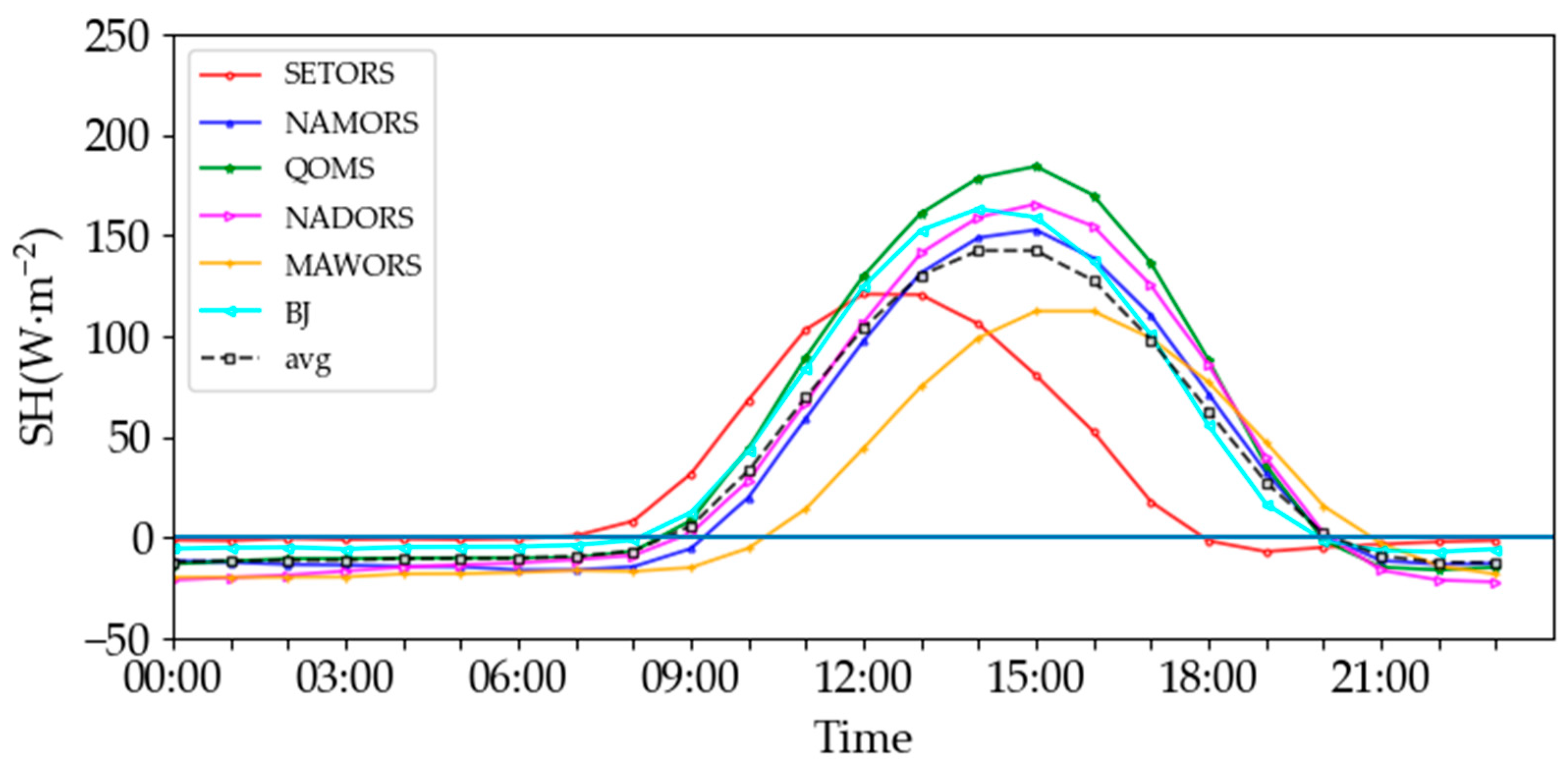
Obvious diurnal variation exists in SH over the TP. Here we adopted the hourly observational SH from the Tibetan Plateau Scientific Data Center to deeply understand the characteristics of the SH diurnal variation over the TP. In addition, the differences between the observed and calculated SH are also examined. The main conclusions are as follows:
(1)
In general, the magnitude of annual mean SH is negative and stable at night, while it is positive with evident variations in the day, and often reaches its peak at around 12:00 or 13:00 local time, except for at SETORS, whose peak appears at around 10:00 local time.
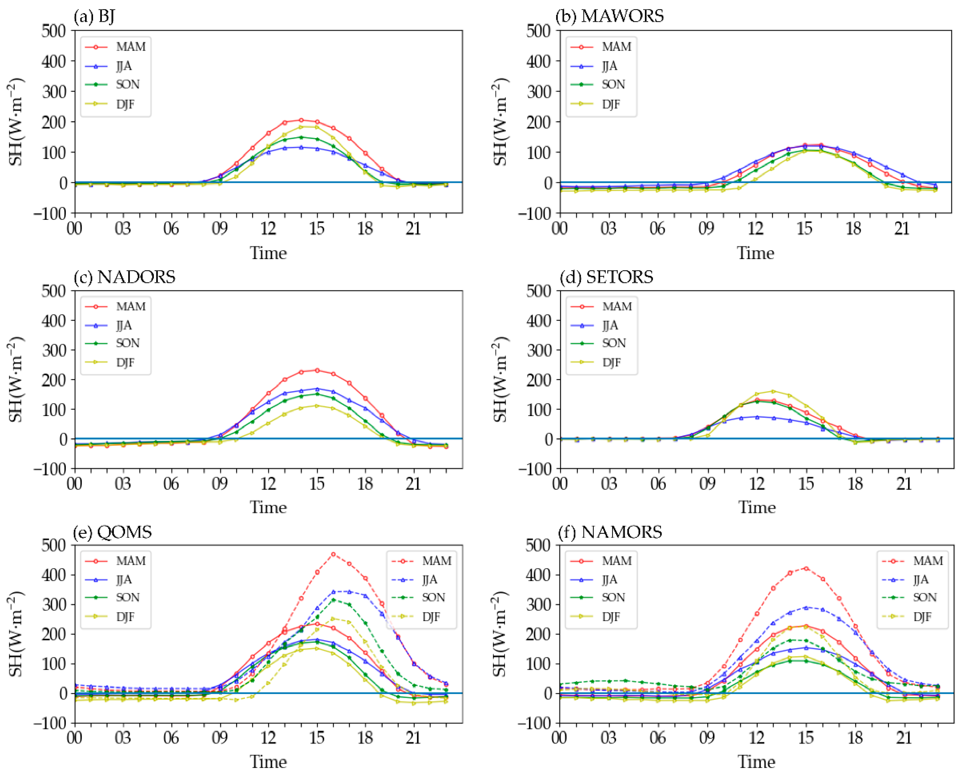
(2)
The SH diurnal variation has obvious seasonal changes, with similar peak timing but different diurnal amplitudes in four seasons at each station. The SH diurnal amplitude is uniformly greatest in spring, followed by summer and autumn, and the smallest in winter at MAWORS, NADORS, and QOMS, while the weakest amplitude in summer and a larger amplitude in winter occur at BJ and SETORS, the strongest amplitude in winter being at SETORS. The peak timing is mostly at 15:00 in four seasons at MAWORS, NADORS, QOMS, and NAMORS, and at 14:00 and 12:00 at BJ and SETORS, respectively.
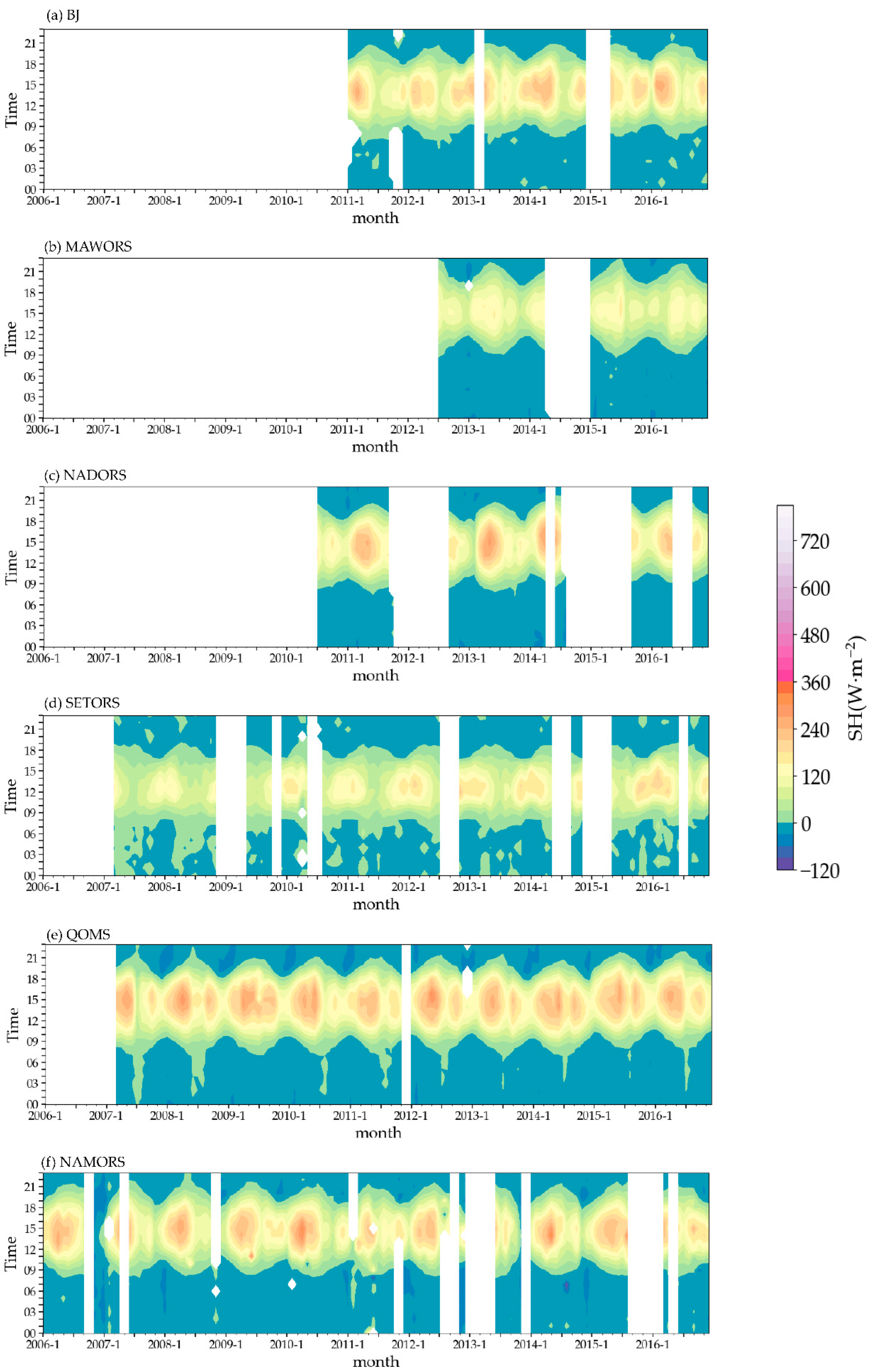
(3)
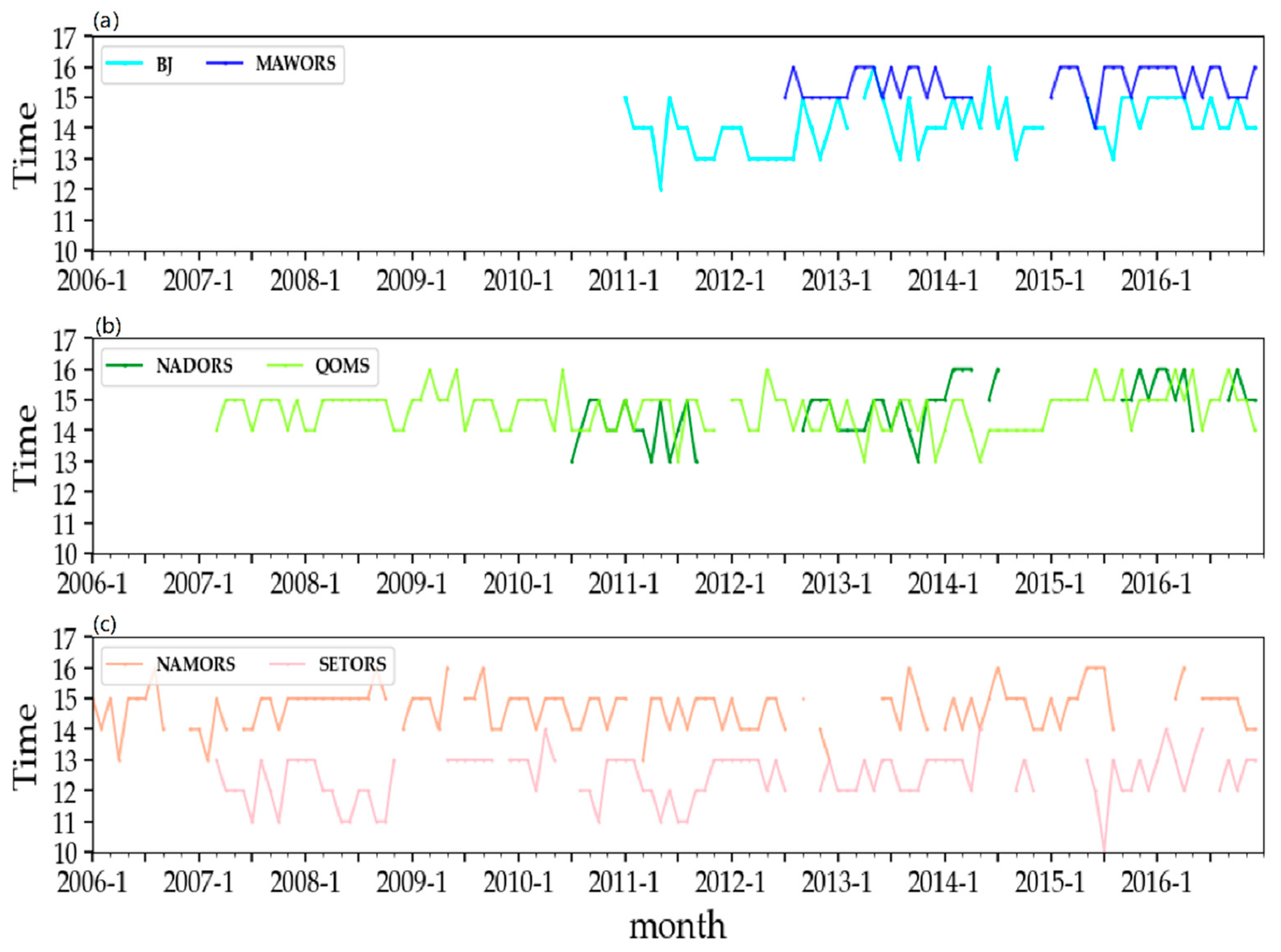
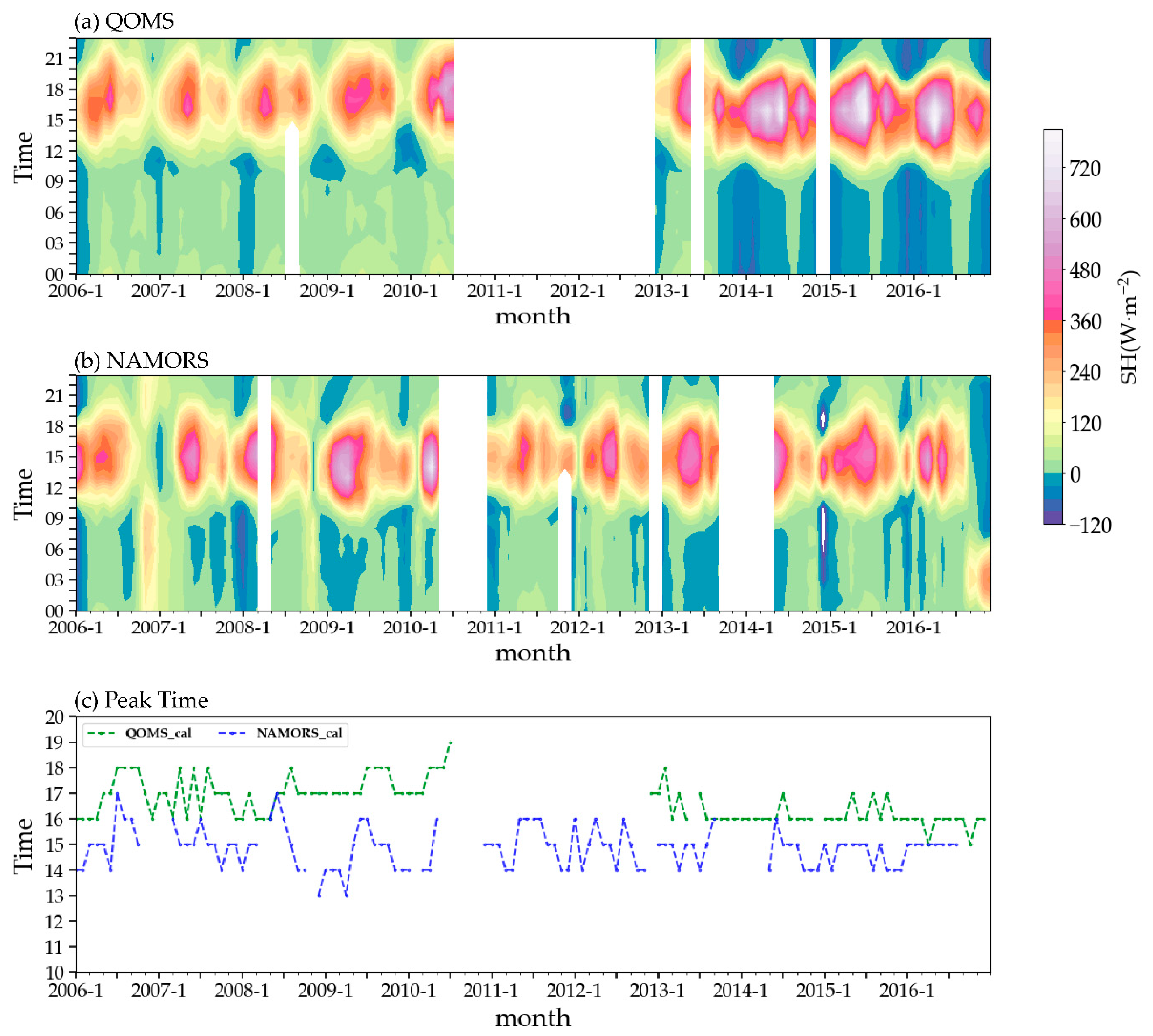
The SH diurnal variation has significant monthly changes. The positive SH at most stations has the longest duration from May to August. The peak timing of SH fluctuates between 15:00 and 16:00 for most months at MAWORS and fluctuates during 12:00–13:00 and 14:00–15:00 at SETORS and NAMORS, respectively. At other stations, the peak timing even shows a shift; for example, at QOMS the peak timing fluctuates between 14:00 and 15:00 before 2015, while it fluctuates between 15:00 and 16:00 after 2015. Moreover, the double-peak phenomenon of SH diurnal variation mainly occurs in spring and autumn, especially at QOMS, which largely contributes to the similar phenomenon in the land–air temperature difference.
(4)
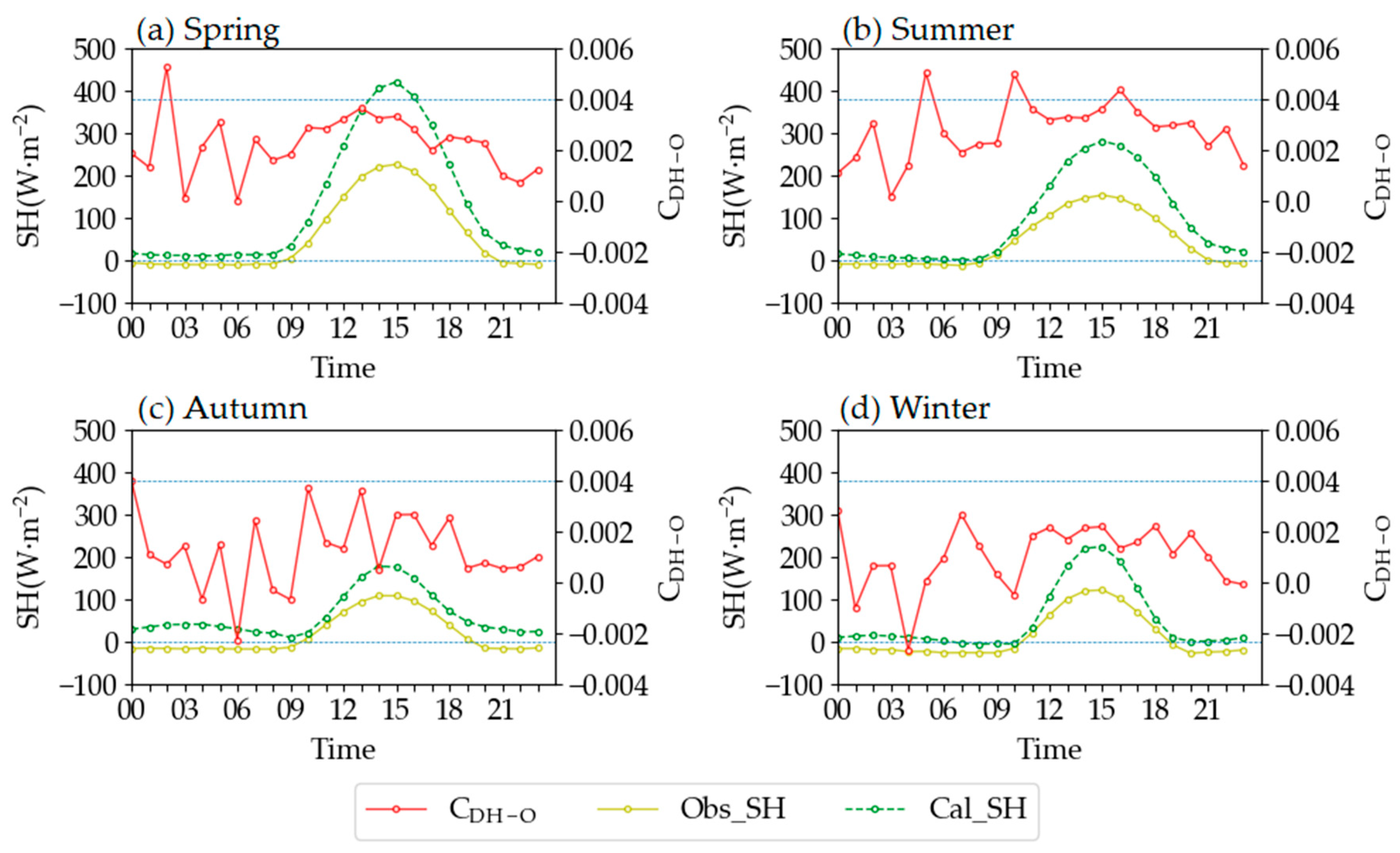
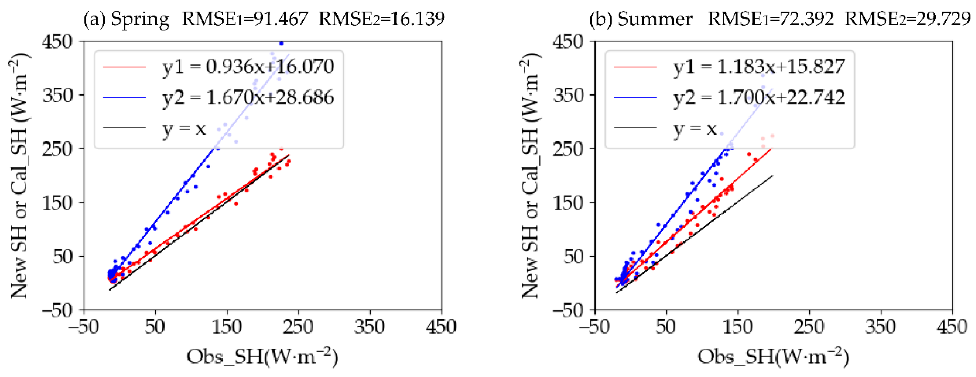
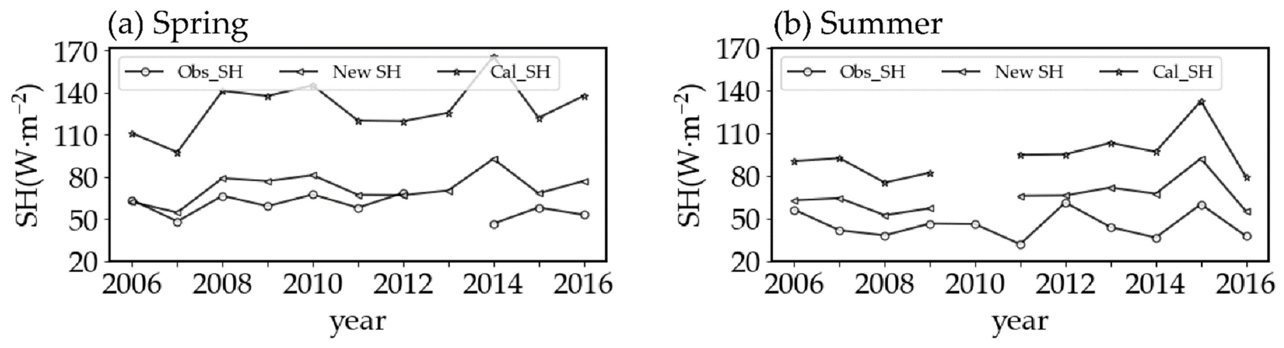
The SH diurnal variations between the observed and calculated SH significantly differ in seasonal and monthly variabilities, including the diurnal amplitude, peak timing, and the range of peak timing fluctuations. For the seasonal mean, the diurnal amplitude of the calculated SH is about 64–100% larger than that of the observed SH. In addition, an obvious phase shift occurs in the peak timing at QOMS, from 15:00 to 16:00. For the monthly changes, the range of the peak timing fluctuations in calculated SH (about 1–3 h) is clearly larger than that in observed SH (about one hour). Furthermore, a new CDH (2.24 × 10⁻³ in spring and 2.78 × 10⁻³ in summer) is recommended here for more accurately calculating TP SH, which may provide a valuable implication for future studies on the TP SH.
Research related to turbulent flux has always been the core issue of land–atmosphere interaction [40], and an in-depth understanding of diurnal variation characteristics in SH over the TP can help us to understand the key land surface processes. Due to the uneven distribution of observations in high mountain regions [28], especially over the TP, the model performance is still poor [41], so various parameterization schemes and numerical models for SH are usually developed. An in-depth understanding of the diurnal variation characteristics of SH over the TP can help to improve and calibrate the numerical modes. Moreover, the new CDH obtained by comparing the calculated SH and observed SH on a diurnal scale can boost the accuracy of SH calculations. However, the impact of the diurnal variation in TP SH on the weather has not been mentioned in this study, and it therefore needs further exploration in the future. It is also worth noting that the suggested new CDH is obtained only from NAMORS due to data limitations, so there is still a certain one-sidedness.

Author Contributions

Conceptualization, M.W.; formal analysis, Z.Z.; writing—original draft, Z.Z.; writing—review and editing, M.W., J.W., X.M., J.L. and X.Y. All authors have read and agreed to the published version of the manuscript.

Funding

This work was sponsored by the National Natural Science Foundation of China (42030605), the Second Tibetan Plateau Scientific Expedition and Research (STEP) program (2019QZKK0105), the National Natural Science Foundation of China (41605039, 41807434, 42030611), the Natural Science Foundation of Jiangsu Province, China (grant no. BK20221449), Meteorological soft science of China Meteorological Administration (2022ZDIANXM28), and the open project of Key Laboratory of Meteorological Disaster (KLME), Ministry of Education & Collaborative Innovation Center on Forecast and Evaluation of Meteorological Disasters (CIC-FEMD), Nanjing University of Information Science & Technology (grant no. KLME202203).

Institutional Review Board Statement

Not applicable.

Informed Consent Statement

Not applicable.

Data Availability Statement

The data presented in this study are openly available in [National Tibetan Plateau Data Center] at [https://doi.org/10.11888/Meteoro.tpdc.270910], reference number [27].

Conflicts of Interest

The authors declare no conflict of interest.

References

  1. Ma, Y.M.; Hu, Z.Y.; Tian, L.D.; Zhang, F.; Duan, A.M.; Yang, K.; Zhang, Y.L.; Yang, Y.P. Study Progresses of the Tibet Plateau Climate System Change and Mechanism of Its Impact on East Asia. Adv. Earth Sci. 2014, 29, 207–215. [Google Scholar]
  2. Wu, G.X.; Liu, Y.M.; Liu, X. How the Heating over the Tibetan Plateau Affects the Asian Climate in Summer. Chin. J. Atmos. Sci. 2005, 29, 47–56. [Google Scholar]
  3. Dai, Y.F. Interannual Variability of Surface Sensible Heat Flux in the Tibetan Plateau and Its Impacts on the Advancing Process of East-Asian Subtropical Summer Monsoon. Master’s Thesis, Nanjing University of Information Science and Technology, Nanjing, China, 2016. [Google Scholar]
  4. Zhang, Y.S.; Wu, G.X. Diagnostic Investigations on the Mechanism of the Onset of Asian Summer Monsoon and Abrupt Seasonal Transitions over the Northern Hemisphere Part: II the Role of Surface Sensible Heating over Tibetan Plateau and Surrounding regions. Acta. Meteor. Sin. 1999, 57, 57–74. [Google Scholar]
  5. Wu, G.X.; Liu, Y.M.; He, B.; Bao, Q.; Wang, Z.Q. Review of the Impact of the Tibetan Plateau Sensible Heat Driven Air-Pump on the Asian Summer Monsoon. Chin. J. Atmos. Sci. 2018, 42, 488–504. [Google Scholar]
  6. Zhou, X.J.; Zhao, P.; Chen, J.M.; Chen, L.X.; Li, W.L. Impacts of thermodynamic processes over the Tibetan Plateau on the Northern Hemispheric climate. Sci. China Ser. D-Earth Sci. 2009, 39, 1473–1486. [Google Scholar] [CrossRef]
  7. Duan, A.M.; Liu, Y.M.; Wu, G.X. Heating status of the Tibetan Plateau from April to June and rainfall and atmospheric circulation anomaly over East Asia in midsummer. Sci. China Ser. D-Earth Sci. 2005, 48, 250–257. [Google Scholar] [CrossRef]
  8. Li, D.L.; Wei, L.; Li, W.J.; Lv, L.Z.; Zhong, H.L.; Ji, G.L. The Effect of Surface Sensible Heat Flux of the Qinghai-Xizang Plateau on General Circulation over the Northern Hemisphere Climatic Anomaly of China. Clim. Env. Res. 2003, 8, 60–70. [Google Scholar]
  9. Zhang, C.C. The Anomaly of the Surface Sensible Heat of the Tibetan Plateau in the Boreal Spring and Its Influences on the Summertime Rainfall Pattern. Master’s Thesis, Nanjing University of Information Science and Technology, Nanjing, China, 2016. [Google Scholar]
  10. Ma, Y.M.; Fan, S.; Ishikawa, H.; Tsukamoto, O.; Yao, T.D.; Koike, T.; Zuo, H.; Hu, Z.Y.; Su, Z.B. Diurnal and inter-monthly variation of land surface heat fluxes over the central Tibetan Plateau area. Theor. Appl. Climatol. 2005, 80, 259–273. [Google Scholar] [CrossRef]
  11. Wang, H.; Zhang, L.; Shi, X.D.; Li, D.L. Seasonal Differences in the Trend Turning Characteristics of Surface Sensible Heat over the Central and Eastern Tibetan Plateau. Chin. J. Atmos. Sci. 2022, 46, 133–150. [Google Scholar]
  12. Xie, J.; Liu, C.; Ge, J. Characteristics of Surface Sensible Heat Flux over the Qinghai-Tibetan Plateau and Its Response to Climate Change. Plateau Meteor. 2018, 37, 28–42. [Google Scholar]
  13. Wang, M.R. Trend in the Atmospheric Heat Source over the Tibetan Plateau and Its Influence on Interdecadal Variation of Summer Precipitation in China during the Past 30 Years. Master’s Thesis, Nanjing University of Information Science and Technology, Nanjing, China, 2016. [Google Scholar]
  14. Duan, L.J.; Duan, A.M.; Hu, W.T.; Gong, Y.F. Low Frequency Oscillation of Precipitation and Daily Variation Characteristic of Air–Land Process at Shiquanhe Station and Linzhi Station in Tibetan Plateau in the Summer of 2014. Chin. J. Atmos. Sci. 2017, 41, 767–783. [Google Scholar]
  15. Ma, Y.M.; Tsukamoto, O.; Wu, X.M.; Tamagawa, I.; Wang, J.M.; Tshikawa, H.; Hu, Z.Y.; Gao, H.C. Characteristics of Energy Transfer and Micrometeorology in the Surface Layer of the Atmosphere above Grassy Marshland of the Tibetan Plateau Area. Chin. J. Atmos. Sci. 2000, 24, 715–722. [Google Scholar]
  16. Liu, Y.; Zou, H.; Hu, F. Observation Study on Atmospheric Surface Layer in Rongbu Valley in Zumolama Peak Area of Qinghai-Xizang Plateau. Plateau Meteor. 2004, 23, 512–518. [Google Scholar]
  17. Li, G.P.; Duan, T.Y.; Gong, Y.F. Bulk Transfer Coefficients and Surface Fluxes over the Western Tibetan Plateau. Chin. Sci. Bull. 2000, 45, 865–869. [Google Scholar]
  18. Li, G.P.; Zhao, B.J.; Lu, J.H. Characteristics of Bulk Transfer Coefficients over the Tibetan Plateau. Acta. Meteor. Sin. 2002, 60, 60–67. [Google Scholar]
  19. Wang, H.; Hu, Z.Y.; Li, D.L.; Dai, Y.F. Estimation of the surface heat transfer coefficient over the east-central Tibetan Plateau using satellite remote sensing and field observation data. Theor. Appl. Climatol. 2019, 138, 169–183. [Google Scholar] [CrossRef]
  20. Chen, W.L.; Wong, D.M. A preliminary study on the computational method of 10-day mean sensible heat and latent heat on the Tibetan Plateau. In Collected Works of the Qinghai-Xizang Plateau Meteorological Experiment; Series 2; Science Press: Beijing, China, 1984. [Google Scholar]
  21. Li, G.P.; Duan, T.Y.; Wan, J.; Gong, Y.F.; Haginoya, S.; Chen, L.X.; Li, W.L. Determination of the drag coefficient over the Tibetan Plateau. Adv. Earth Sci. 1996, 13, 511–518. [Google Scholar]
  22. Wang, M.R.; Zhou, S.W.; Duan, A.M. Trend in the atmospheric heat source over the central and eastern Tibetan Plateau during recent decades: Comparison of observations and reanalysis data. Chin. Sci. Bull. 2012, 57, 178–188. [Google Scholar] [CrossRef] [Green Version]
  23. Li, C.F.; Yanai, M. the Onset and Interannual Variability of the Asian Summer Monsoon in Relation to Land–Sea Thermal Contrast. J. Clim. 1996, 9, 358–375. [Google Scholar] [CrossRef]
  24. Wang, T.Z.; Zhao, Y. Comparative analysis of five sets of surface sensible heat flux data over the Tibetan Plateau in May. J. Meteor. Sci. 2020, 40, 819–828. [Google Scholar]
  25. Shan, X.; Zhou, S.W.; Wang, M.R.; Zheng, D.; Wang, C.H. Effects of Spring Sensible Heat in the Tibetan Plateau on Midsummer Precipitation in South China under ENSO. J. Trop. Meteor. 2020, 36, 60–71. [Google Scholar]
  26. Chen, L.; Pryor, S.C.; Wang, H.; Zhang, R.H. Distribution and Variation of the Surface Sensible Heat Flux over the Central and Eastern Tibetan Plateau: Comparison of Station Observations. J. Geophys. Res. Atmos. 2019, 124, 6191–6206. [Google Scholar] [CrossRef]
  27. Ma, Y.M. A Long-Term Dataset of Integrated Landatmosphere Interaction Observations on the Tibetan Plateau (2005–2016); National Tibetan Plateau Data Center: Beijing, China, 2020. [Google Scholar]
  28. Ma, Y.M.; Hu, Z.Y.; Xie, Z.P.; Ma, W.Q.; Wang, B.B.; Chen, X.L.; Li, M.S.; Zhong, L.; Sun, F.L.; Gu, L.L.; et al. A long-term (2005–2016) dataset of hourly integrated land–atmosphere interaction observations on the Tibetan Plateau. Earth Syst. Sci. Data. 2020, 12, 2937–2957. [Google Scholar] [CrossRef]
  29. Duan, A.M.; Li, F.; Wang, M.R.; Wu, G.X. Persistent weakening trend in the spring sensible heat source over the Tibetan Plateau and its impact on the Asian summer monsoon. J. Clim. 2011, 24, 5671–5682. [Google Scholar] [CrossRef] [Green Version]
  30. Zhu, L.H.; Huang, G.; Fan, G.Z.; Qu, X.; Zhao, G.J.; Hua, W. Evolution of surface sensible heat over the Tibetan Plateau under the recent global warming hiatus. Adv. Atmos. Sci. 2017, 34, 1249–1262. [Google Scholar] [CrossRef]
  31. Wang, H.; Zhang, L.; Shi, X.D.; Li, D.L. Some New Changes of the Regional Climate on the Tibetan Plateau Since 2000. Adv. Earth Sci. 2021, 36, 785–796. [Google Scholar]
  32. Duan, A.M.; Wu, G.X. Weakening Trend in the Atmospheric Heat Source over the Tibetan Plateau during Recent Decades. Part I: Observations. J. Clim. 2008, 21, 3149–3164. [Google Scholar] [CrossRef] [Green Version]
  33. Ye, D.Z.; Gao, Y.X.; Zhou, M.Y. Qinghai-Xizang Plateau Meteorology; Science Press: Beijing, China, 1979. [Google Scholar]
  34. Yu, J.H.; Liu, J.M.; Ding, Y.G. Annual and Diurnal Variations of Surface Fluxes in Western Qinghai-Xizang Plateau. Plateau Meteor. 2004, 23, 353–359. [Google Scholar]
  35. Ji, J.J.; Huang, M. The Estimation of the Surface Energy Fluxes over Tibetan Plateau. Adv. Earth Sci. 2006, 21, 1268–1272. [Google Scholar]
  36. Jin, R.; Qi, L.; He, J.H. Effect of oceans to spring surface sensible heat flux over Tibetan Plateau and its influence to East China precipitation. Acta Oceanol. Sin. 2016, 38, 83–95. [Google Scholar]
  37. Wang, X.J.; Yang, M.X.; Wan, G.N. Temporal-Spatial Distribution and Evolution of Surface Sensible Heat Flux over Qinghai-Xizang Plateau during Last 60 Years. Plateau Meteor. 2013, 32, 1557–1567. [Google Scholar]
  38. Duan, A.M.; Liu, S.F.; Hu, W.T.; Hu, D.; Peng, Y.Z. Long-term daily dataset of surface sensible heat flux and latent heat release over the Tibetan Plateau based on routine meteorological observations. Big Earth Data 2022, 6, 480–491. [Google Scholar] [CrossRef]
  39. Zhu, Y.X.; Ding, Y.H.; Liu, W.H. Simulation of the Influence of Winter Snow Depth over the Tibetan Plateau on Summer Rainfall in China. Chin. J. Atmos. Sci. 2009, 33, 903–915. [Google Scholar]
  40. Duan, L.J. Characteristics of Multiscale Air-Land Interaction over Tibetan Plateau in the Summer of 2014. Master’s Thesis, Chengdu University of Information Science and Technology, Chengdu, China, 2017. [Google Scholar]
  41. Xie, Z.P.; Hu, Z.Y.; Ma, Y.M.; Sun, G.H.; Gu, L.L.; Liu, S.; Wang, Y.D.; Zheng, H.X.; Ma, H.Q. Modeling Blowing Snow over the Tibetan Plateau with the Community Land Model: Method and Preliminary Evaluation. J. Geophys. Res.-Atmos. 2019, 124, 9332–9355. [Google Scholar] [CrossRef]
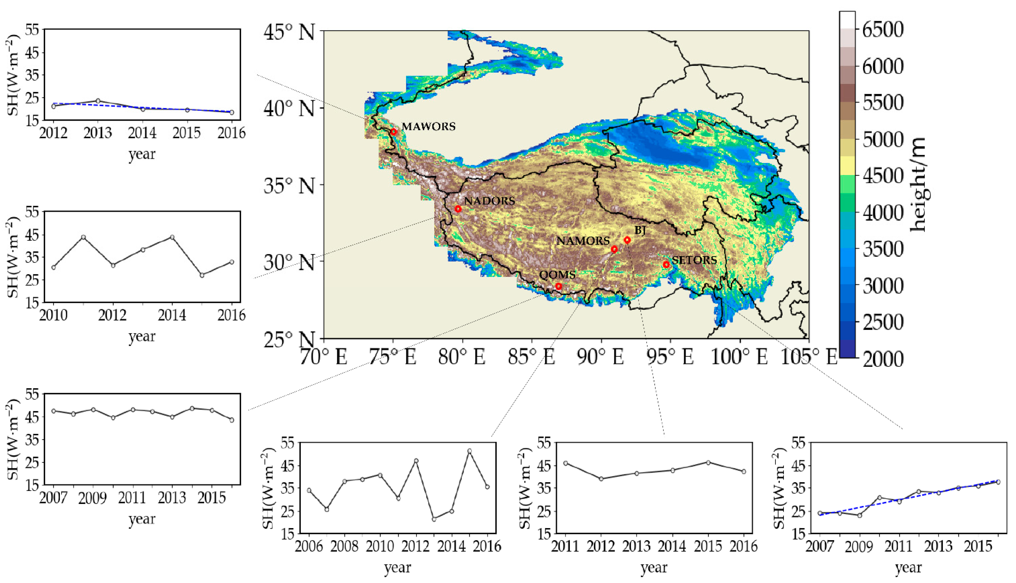
Figure 1. Geographical distributions of the six meteorological stations over the TP and the time series of the annual mean SH (units: W m−2) at these six stations during the period 2006–2016. The blue dotted lines indicate the decreasing and increasing trends at MAWORS and SETORS, respectively.
Atmosphere 14 00128 g001
Figure 2. Climatological annual mean of diurnal variations of the observed SH (W m−2) at six stations over the TP during the period 2006–2016. The colored lines represent SH at the six stations, respectively, and the black line indicates their average. The time in x axis is Beijing time.
Atmosphere 14 00128 g002
Figure 3. Climatological seasonal mean of the diurnal variation of the observed SH (solid lines, W m−2) at (a) BJ, (b) MAWORS, (c) NADORS, (d) SETORS, (e) QOMS, and (f) NAMORS, and the calculated SH (dashed lines, W m−2) at (e) QOMS and (f) NAMORS.
Atmosphere 14 00128 g003
Figure 4. Monthly mean of the diurnal variation in observed SH (shaded, W m−2) at (a) BJ, (b) MAWORS, (c) NADORS, (d) SETORS, (e) QOMS, and (f) NAMORS during the period 2006–2016.
Atmosphere 14 00128 g004
Figure 5. Peak timing (hour) of monthly diurnal variation in SH at (a) BJ and MAWORS, (b) NADORS and QOMS, and (c) NAMORS and SETORS.
Atmosphere 14 00128 g005
Figure 6. Monthly mean of the diurnal variation in (a) land–air temperature difference (Ts-Ta, unit: °C) and (b) wind speed at the height of 10 m (V10, unit: m/s) at QOMS during the period 2006–2016.
Atmosphere 14 00128 g006
Figure 7. Monthly mean of the diurnal variation in calculated SH (shaded, W m−2) at (a) QOMS and (b) NAMORS during the period 2006–2016. The curve lines in (c) represent the peak timing (hour) of monthly SH diurnal variation at each station, respectively.
Atmosphere 14 00128 g007
Figure 8. Seasonal mean of the diurnal variation in the derived heat transfer coefficient (CDH-O), observed SH (Obs_SH, unit: W m−2) and calculated SH (Cal_SH, unit: W m−2) at NAMORS in (a) spring, (b) summer, (c) autumn, and (d) winter. The two horizontal dashed lines indicate zero SH and 0.004 CDH-O, respectively.
Atmosphere 14 00128 g008
Figure 9. The relationship between the originally calculated SH and observed SH (blue lines, unit: W m−2), and between the new SH and observed SH (red lines, unit: W m−2) in the seasonal mean of the diurnal variation in (a) spring and (b) summer at NAMORS. RMSE1 and RMSE2 denote the root mean squared error of the originally calculated SH and the new SH, respectively.
Atmosphere 14 00128 g009
Figure 10. Time series of the annual mean in observed SH (Obs_SH, units: W m−2), originally calculated SH (Cal_SH, units: W m−2), and new SH (New SH, units: W m−2) in (a) spring and (b) summer at NAMORS during the period 2006–2016.
Atmosphere 14 00128 g010
Table 1. List of the stations in the hourly integrated observational dataset, including the station names, latitudes, longitudes, time periods, and the time difference between local time and Beijing time.
StationLatitudeLongitudeTime PeriodTime Difference between Local Time and Beijing Time
(Local Time Is Later than Beijing Time)
BJ31.37° N91.90° E2011–20161 h 52 min late
QOMS28.36° N86.95° E2007–20162 h 12 min late
SETORS29.77° N94.73° E2007–20161 h 41 min late
NAMORS30.77° N90.98° E2006–20161 h 56 min late
NADORS33.39° N79.70° E2010–20162 h 41 min late
MAWORS38.41° N75.05° E2012–20163 h 00 min late
Table 2. The month and the specific timing of the occurrence of the two large centers in SH diurnal variation at six stations from 2006 to 2016.
QOMSBJ
Month1 (Time)Month2 (Time)Month1 (Time)Month2 (Time)
2006
2007May (15:00)October (15:00)
2008April (15:00)September (15:00)
2009April (15:00)October (15:00)
2010June (16:00)October (15:00)
2011May (15:00)September (15:00)March (14:00)December (14:00)
2012May (16:00)October (14:00)February (14:00)October (14:00)
2013May (15:00)September (15:00) December (14:00)
2014June (14:00)September (14:00)May (14:00)November (14:00)
2015June (16:00)September (16:00) October (15:00)
2016April (15:00)October (15:00)March (15:00)November (14:00)
MAWORSSETORSNADORSNAMORS
Month1 (Time)Month1 (Time)Month1 (Time)Month1 (Time)
2006 April (13:00)
2007 March (13:00)
2008 February (13:00) April (15:00)
2009 April (14:00)
2010 January (13:00) April (15:00)
2011 February (13:00)May (15:00)May (15:00)
2012 February (13:00) May (15:00)
2013April (16:00)February (12:00)May (15:00)
2014March (15:00) May (14:00)
2015May (15:00) May (16:00)
2016July (16:00)February (14:00)
Disclaimer/Publisher’s Note: The statements, opinions and data contained in all publications are solely those of the individual author(s) and contributor(s) and not of MDPI and/or the editor(s). MDPI and/or the editor(s) disclaim responsibility for any injury to people or property resulting from any ideas, methods, instructions or products referred to in the content.

