Article

Application of a Hybrid CEEMD-LSTM Model Based on the Standardized Precipitation Index for Drought Forecasting: The Case of the Xinjiang Uygur Autonomous Region, China

1
School of Geography, Nanjing Normal University, Nanjing 210023, China
2
Ningbo Yinzhou Planning & Design Institute, Ningbo 315192, China
*
Author to whom correspondence should be addressed.
Atmosphere 2022, 13(9), 1504; https://doi.org/10.3390/atmos13091504
Submission received: 19 August 2022 / Revised: 7 September 2022 / Accepted: 12 September 2022 / Published: 15 September 2022
(This article belongs to the Section Atmospheric Techniques, Instruments, and Modeling)

Abstract

:
Accurate forecasting of droughts can effectively reduce the risk of drought. We propose a hybrid model based on complementary ensemble empirical mode decomposition (CEEMD) and long short-term memory (LSTM) to improve drought prediction accuracy. Taking the Xinjiang Uygur Autonomous Region as an example, the prediction accuracy of the LSTM and CEEMD-LSTM models for the standardized precipitation index (SPI) on multiple timescales was compared and analyzed. Multiple evaluation metrics were used in the comparison of the models, such as the Nash–Sutcliffe efficiency (NSE). The results show that (1) with increasing timescale, the prediction accuracy of the LSTM and CEEMD-LSTM models gradually improves, and both reach their highest accuracy at the 24-month timescale; (2) the CEEMD can effectively stabilize the time-series, and the prediction accuracy of the hybrid model is higher than that of the single model at each timescale; and (3) the NSE values for the hybrid CEEMD-LSTM model at SPI24 were 0.895, 0.930, 0.908, and 0.852 for Fuhai, Kuerle, Yutian, and Hami station, respectively. This indicates the applicability of the hybrid model in the forecasting of drought.

1. Introduction

Drought is one of the most serious meteorological disasters, causing increasing damage to agricultural production, economic operations, and modern life [1,2]. Furthermore, the frequency and intensity of widespread droughts is expected to increase. Easy-to-compute drought indicators are often used to monitor and assess the extent, duration, and impact of drought [3,4,5,6]. Due to the wide range of applications and the different understandings of drought in different disciplines, various drought indicators have been proposed and applied in drought prediction.
Common drought indices include the standardized precipitation index (SPI) [7,8,9], standardized precipitation evapotranspiration index (SPEI) [10,11,12], Palmer drought severity index (PDSI) [13,14], and reconnaissance drought index (RDI) [15,16]. Among these, the SPI can be used for drought analysis at various timescales. Furthermore, it has high accuracy in drought classification and can be calculated using only precipitation data [17,18]. As the SPI is widely used in drought research and can be calculated using only precipitation data, it was chosen for use in this study to illustrate the applicability of models in drought prediction.
Precipitation data and the SPI time-series have non-stationary and non-linear characteristics, but traditional data-driven models, such as the autoregressive and moving average (ARMA) model, cannot predict non-linear data very well. Therefore, artificial neural networks (ANNs) have been used in the study of drought prediction [19], and good prediction results have been obtained. With the development of machine learning, the long short-term memory (LSTM) network has been applied in the time-series prediction of drought and its related fields [11,20,21]. LSTM has been proposed to solve the long-term dependency problem and thus has advantages in handling sequences with long intervals and delays [22]. However, a single model is prone to a local optimum in the prediction of time-series, and the prediction effect is not satisfactory. Therefore, many scholars have introduced the decomposition of signals in the prediction of time-series [23,24]. Signal decomposition can extract the local features of the sequence and make the sequence stable. Scholars in related disciplines have decomposed time-series using empirical mode decomposition (EMD) [22], ensemble empirical mode decomposition (EEMD) [25], and complementary ensemble empirical mode decomposition (CEEMD) [26]. These decomposition methods reduce the complexity of the original time-series and improve the predictability of the data. The original series is decomposed into a set of more stable components and a trend term. Among the above three decomposition methods, CEEMD solves the modal mixing problem of EMD and the residual white noise problem of EEMD. Johny et al. [27] used multivariate EMD-LSTM for predicting monthly rainfall in India, and the prediction results showed that the model is superior to ANN hybrids in the prediction of mean and extreme rainfall.
As mentioned above, with the non-linear and non-stationary characteristics of precipitation data and the advantages of LSTM in long time-series prediction, a hybrid model is proposed to improve prediction accuracy in drought prediction. Taking the Xinjiang Uygur Autonomous Region as an example, the main objectives of the present study are as follows: (1) to characterize drought conditions using the SPI at 1-, 3-, 6-, 9-, 12-, and 24-month timescales; (2) to develop the LSTM and propose a hybrid model by combining it with the advantages of CEEMD in dealing with non-linear, non-stationary time-series; and (3) to evaluate the efficiency of the LSTM and CEEMD-LSTM models based on the Kruskal–Wallis test, statistical criteria, and the Kriging interpolation method.

2. Materials and Methods

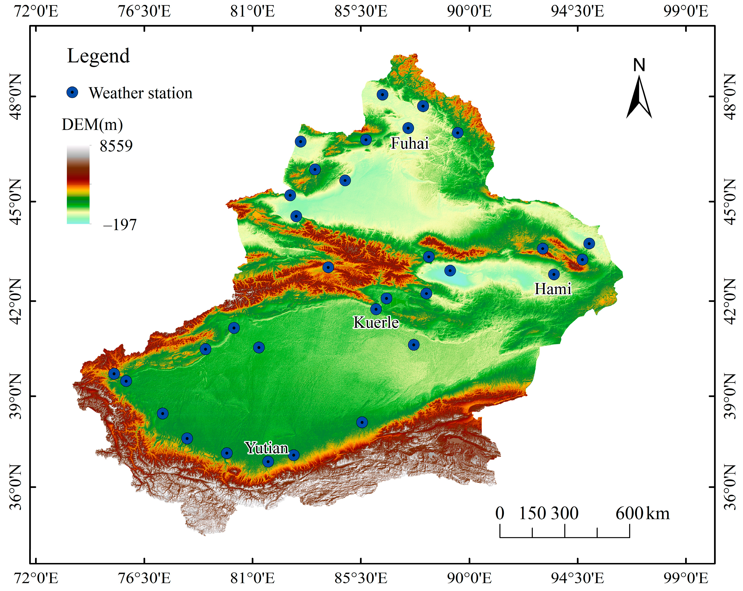
2.1. Study Area and Data

The Xinjiang Uygur Autonomous Region is the largest provincial-level administrative region in China in terms of area. It ranges from 73°40′ E to 96°18′ E and from 34°25′ N to 48°10′ N, with an average altitude of about 1000 m (Figure 1). The region is far from the sea and deep inland, with low precipitation levels and a dry climate. The average annual precipitation in Xinjiang is about 150 mm, but there is a large difference between the annual precipitation in the northern and southern regions, with only 20–100 mm in the southern region and 100–500 mm in the northern region. Furthermore, the temperature in the south of Xinjiang is higher than that in the north, with an annual average temperature of 10–13 °C in the south and one below 10 °C in the north. Xinjiang was used as the study area due to its large area. Furthermore, the main purpose of this study was to investigate the applicability of CEEMD-LSTM for drought prediction. Therefore, four meteorological stations located in the northern, southern, eastern, and central parts of the region were selected as examples to display the SPI calculation values and the predicted values of the two models. The original data were obtained from the National Meteorological Data Center (http://data.cma.cn/ accessed on 13 March 2020).

2.2. Methods

2.2.1. Standardized Precipitation Index

The SPI was developed by McKee et al. [28] and has been recommended by the World Meteorological Organization [29]. It is calculated based on precipitation data only. SPI values on 1-, 3-, 6-, 9-, 12-, and 24-month timescales can be used to describe meteorological drought, agricultural drought, and hydrological drought conditions in a region [30,31,32]. The calculation process of the SPI is as follows:
SPI = B   ( t c 0 + c 1 t + c 2 t 2 1 + d 1 t + d 2 t 2 + d 3 t 3 ) ,
where B is the positive and negative coefficient of probability density; for B = 1 , t = l n 1 G ( x ) 2 , and for   B = 1 , t = l n 1 ( 1 G ( x ) ) 2 , where G ( x ) is a cumulative probability [33]. The values of the constants are c 0 = 2.515517, c 1 = 0.802853, c 2 = 0.010328, d 1 = 1.432788, d 2 = 0.189269, and d 3 = 0.001308. The drought classification based on SPI values is shown in Table 1.

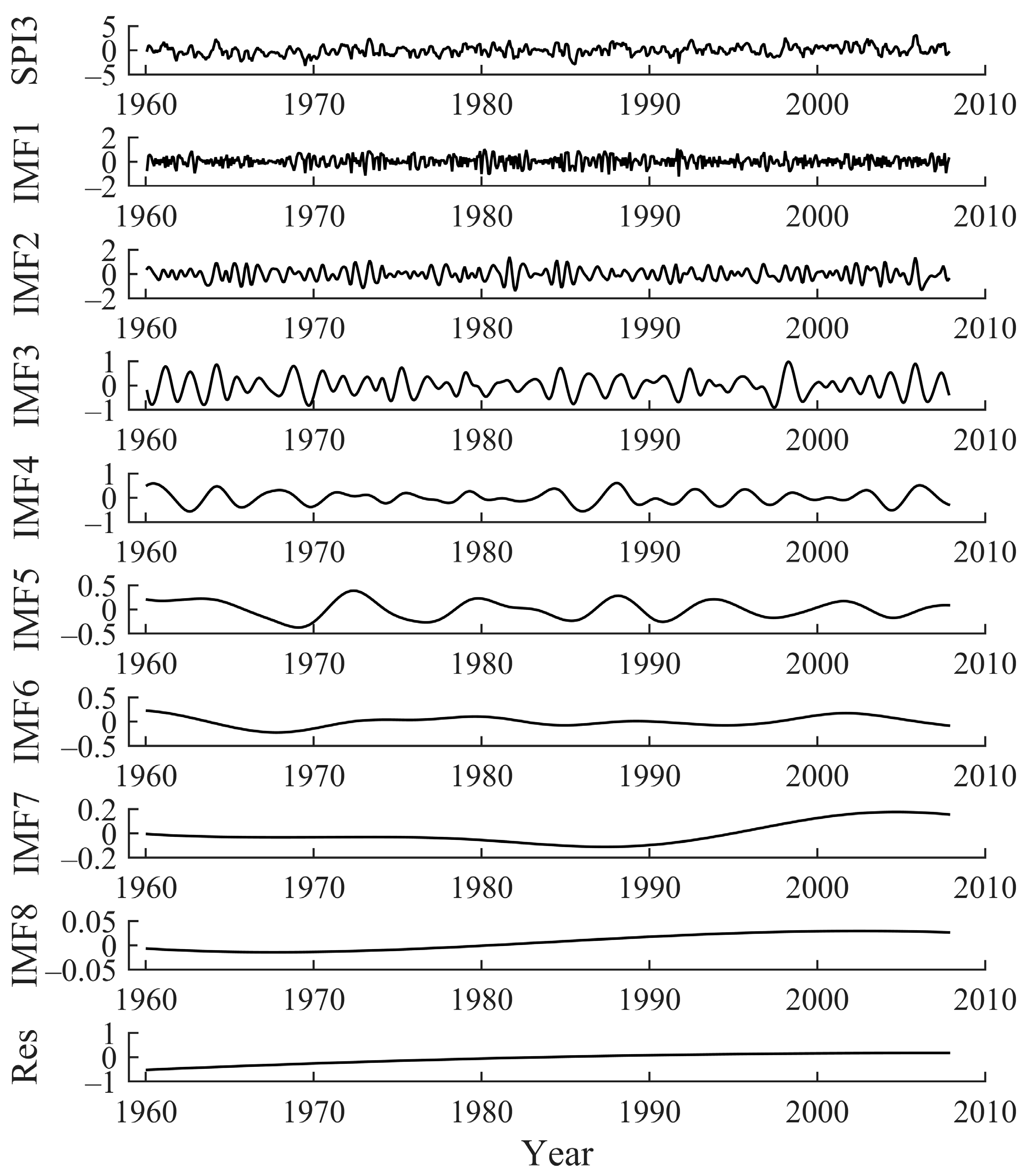
2.2.2. Complementary Ensemble Empirical Mode Decomposition

As proposed by Yeh et al. [34], CEEMD is able to decompose the original sequence to obtain a set of intrinsic mode function (IMF) and trend terms. It has obvious advantages in handling time-frequency sequences of non-linear and non-stationary signals. The components contain the local features of the original sequence at different scales. The algorithm steps are described below.
First, n groups of auxiliary white noise, including positive and negative noise, are added to the original sequence B(t):
[   H 1   H 2   ] = [   1 1 1 1   ] [   B N   ] ,
where N is an auxiliary sequence, and H1 and H2 are positive noise and negative noise sequences, respectively. Then, the obtained sequences are decomposed by EMD to obtain m IMF components, and each set of components is denoted as C i j + ( t ) and C i j ( t ) , where i = 1, …, n and j = 1, …, m. The value of IMF j is obtained according to the following formula:
IMF j = 1 2 n i = 1 n ( C i j + ( t ) + C i j ( t ) ) .
The obtained IMF values are used as the final decomposition results. The original sequence is decomposed into:
B ( t ) = j = 1 m IMF j ( t ) + r ( t )
where r ( t ) is a residual trend quantity.

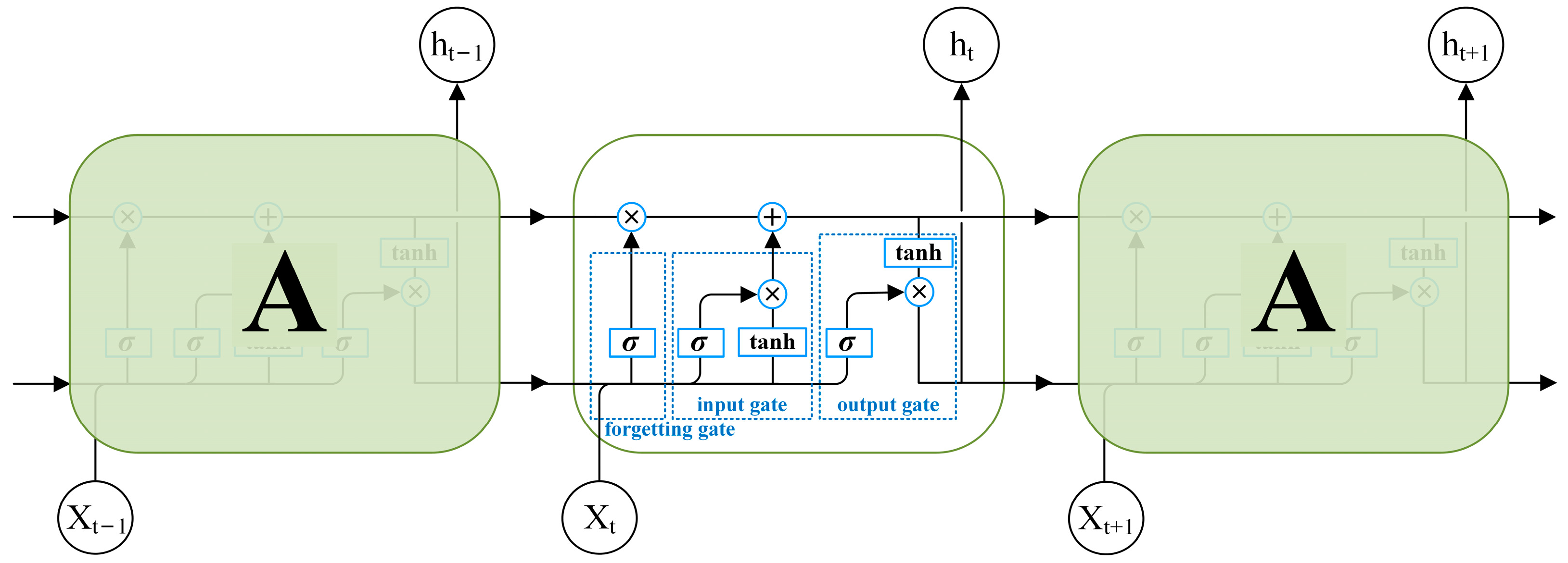
2.2.3. Long Short-Term Memory

As proposed by Hochreiter et al. [35], the LSTM network is a special type of recurrent neural network (RNNs) that is able to learn long-term dependent information in data transmission and can effectively solve the gradient problem. The LSTM network has a more complicated repetition module than RNN, as shown in Figure 2, where Xt is the input sequence at time t, ht is the output of the LSTM network cells at time t, and σ and tanh are the sigmoid activation function and tanh activation function, respectively. The cell state is the key to this repetitive chain of neural network modules. The cell state is the horizontal line that runs through each module, and it ensures the invariance of the information transfer. It is similar to a conveyor belt that runs through the entire chain. Through the “gate” structure, cell state information is added or removed. The “forgetting gate” determines what information is removed from the cell state. The “input gate” determines what information is stored in the cell state. The “output gate” uses a sigmoid layer to determine the portion of the cell state to be output [22]. After the operation (the circle part of Figure 2), the result is passed to the next unit structure.

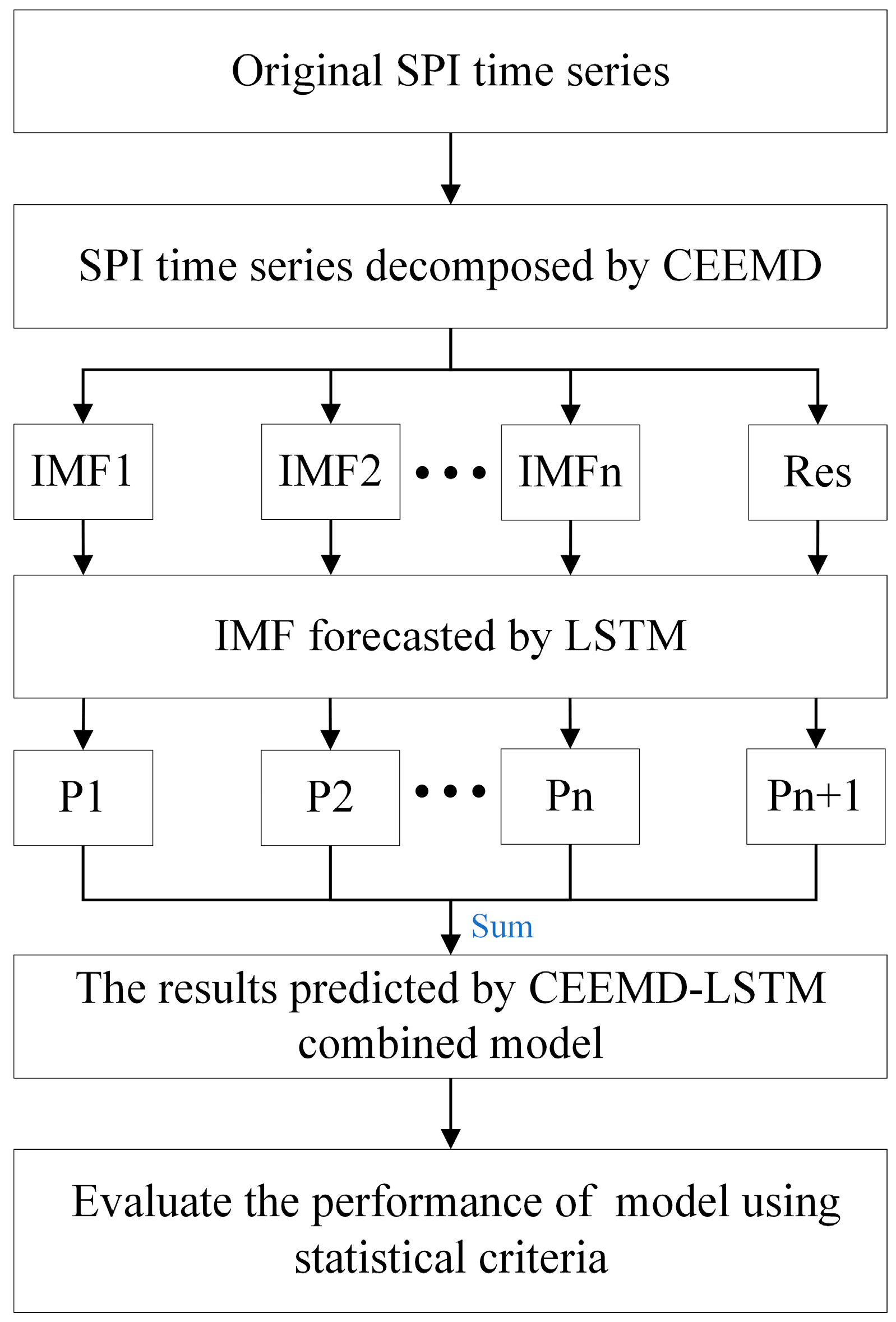
2.2.4. Framework of the Hybrid CEEMD-LSTM Model

The workflow of the hybrid model proposed in this paper is shown in Figure 3. The main processes of forecasting through the hybrid model are as follows:
(1) The CEEMD is used to decompose the original SPI sequence into several subsequences and a residual sequence;
(2) The decomposed sequence is predicted using the LSTM network;
(3) Finally, the predicted SPI sequences are obtained by merging the predicted subsequences and residual error.

2.2.5. Evaluation Metrics

In this study, the Kruskal–Wallis test was used to evaluate the accuracy of the estimated values of the two models. When the p-value ≤ 0.05, there is a difference between the estimated and actual values. Four statistical criteria, including root mean square error (RMSE), mean absolute error (MAE), Willmott index (WI), and Nash-Sutcliffe efficiency (NSE), were used to evaluate the performance of the models. The model with the lowest RMSE and MAE as well as the highest WI and NSE was proposed as the appropriate model. The formulas for the above criteria are as follows:
R M S E = 1 N i = 1 N ( y i y i ^ ) 2
M A E = 1 N i = 1 N | y i y i ^ |
W I = | 1 [ i = 1 N ( y i y i ^ ) 2 i = 1 N ( | y i y ¯ | + | y i ^ y ¯ | ) 2 ] |
N S E = 1 i = 1 N ( y i y i ^ ) 2 i = 1 N ( y i y ¯ ) 2
where y i is the observed value, y ¯ is the average value of y i , y i ^ is the forecasted value, and N is the total data size of y i .

3. Results and Discussion

The calculation of the SPI and the fitting of the LSTM were both accomplished on the Python 3.7 platform.

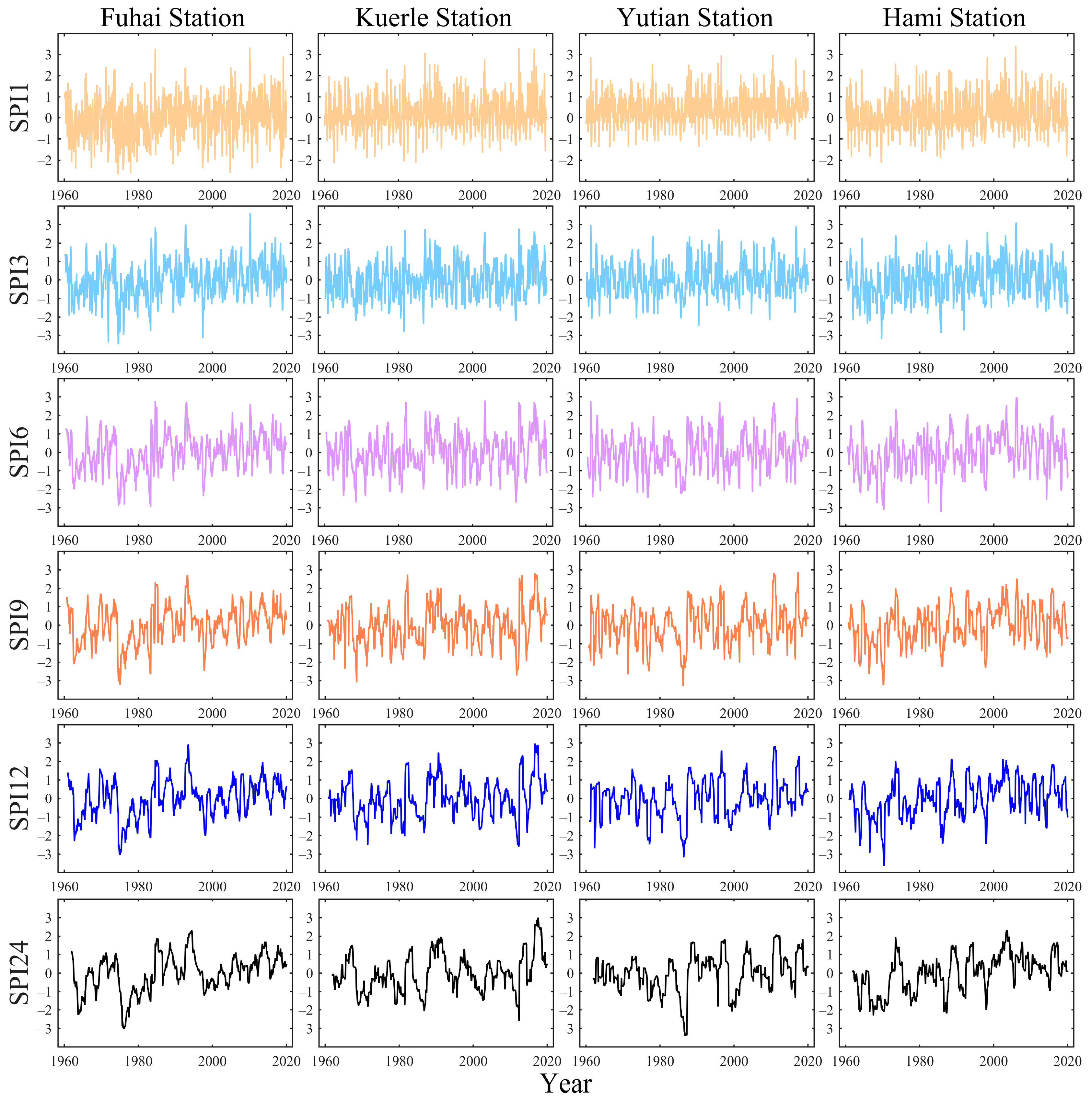
3.1. SPI Values at Different Time Scales

The 1-, 3-, 6-, 9-, 12-, and 24-month timescale SPI values were calculated using daily precipitation data from 32 meteorological stations in the Xinjiang Uygur Autonomous Region during the period of 1960–2019. The results of the multi-timescale SPI for the four example stations are shown in Figure 4. It can be seen that the SPI3, SPI6, SPI9, SPI12, and SPI24 values of the four stations show an increasing trend, especially at Fuhai station, and the frequency of extreme drought decreases over time. In the past decade, there were fewer occurrences of extreme drought at the four stations.
Through the Mann–Kendall trend test (Table 2), it became clear that all SPI sequences at the four stations have an increasing trend, except for SPI1 at the Kuerle station. The precipitation in Xinjiang has increased significantly since the mid-1980s, which caused the SPI values to increase.

3.2. LSTM Modeling and Prediction

In this study, based on 1-, 3-, 6-, 9-, 12-, and 24-month timescale SPI values, LSTM modeling was performed and the SPI dataset was divided by grid search and cross-validation. A total of 80% of the data (1960–2007) were selected as the training set and 20% (2008–2019) were selected as the test set.
Before the data are input into the LSTM model for prediction, it needs to be normalized to eliminate the effect of data dimensionality differences and to improve the model training speed. The common activation functions for LSTM networks are sigmoid, tanh, and ReLU [36,37,38]. However, as the layers of the neural network deepen, the gradient tends to disappear in the backpropagation when using the sigmoid function, and the stochastic gradient descent converges slowly when using the sigmoid or tanh. Therefore, ReLU was chosen as the activation function in this paper. The batch size was set to 1, which means that the model weights were updated after each sample. The hidden layer was composed of 25 storage units, and the loss function was the mean squared error (MSE). To prevent overfitting of the model training, the early stopping method was used during the simulation. Specifically, as the number of iterations increased, the MSE gradually decreased and the model accuracy improved. When the MSE value started to increase, the training was stopped. At this point, the model accuracy was at its highest. To ensure that the accuracy of the model could be maximized, the number of iterations was set to 300. The prediction results of the LSTM are shown in Figure 5, Figure 6, Figure 7 and Figure 8.

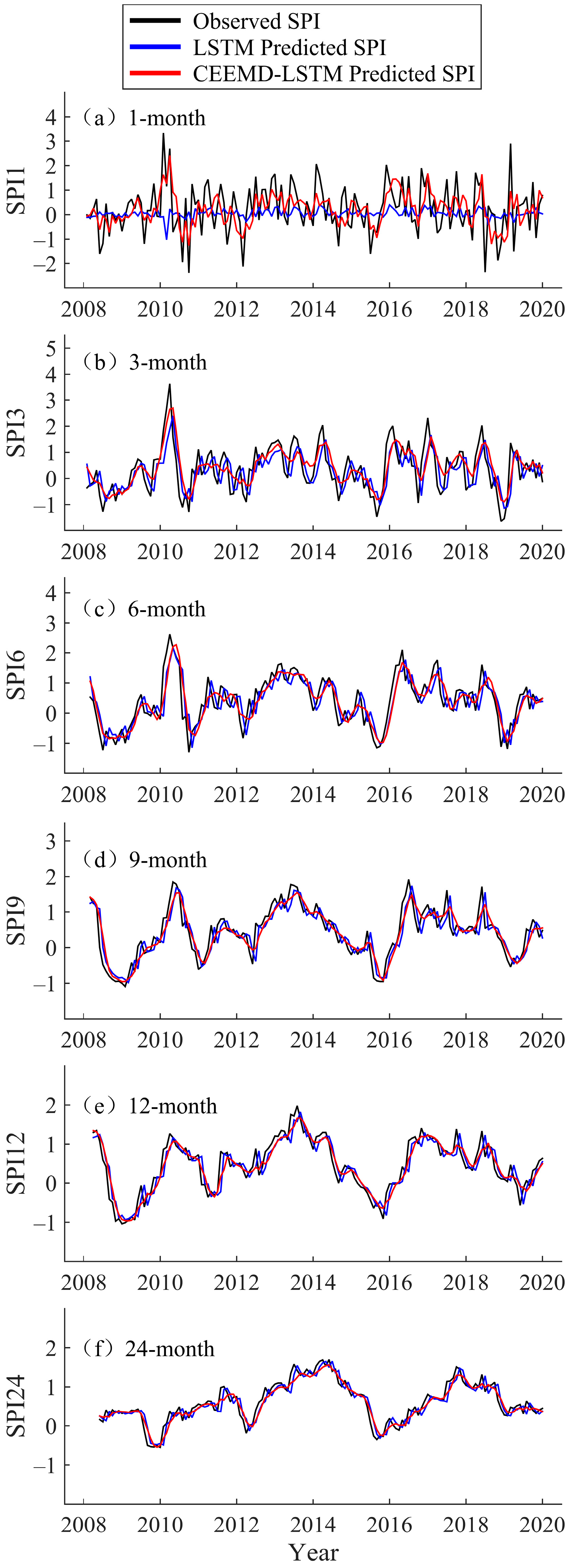
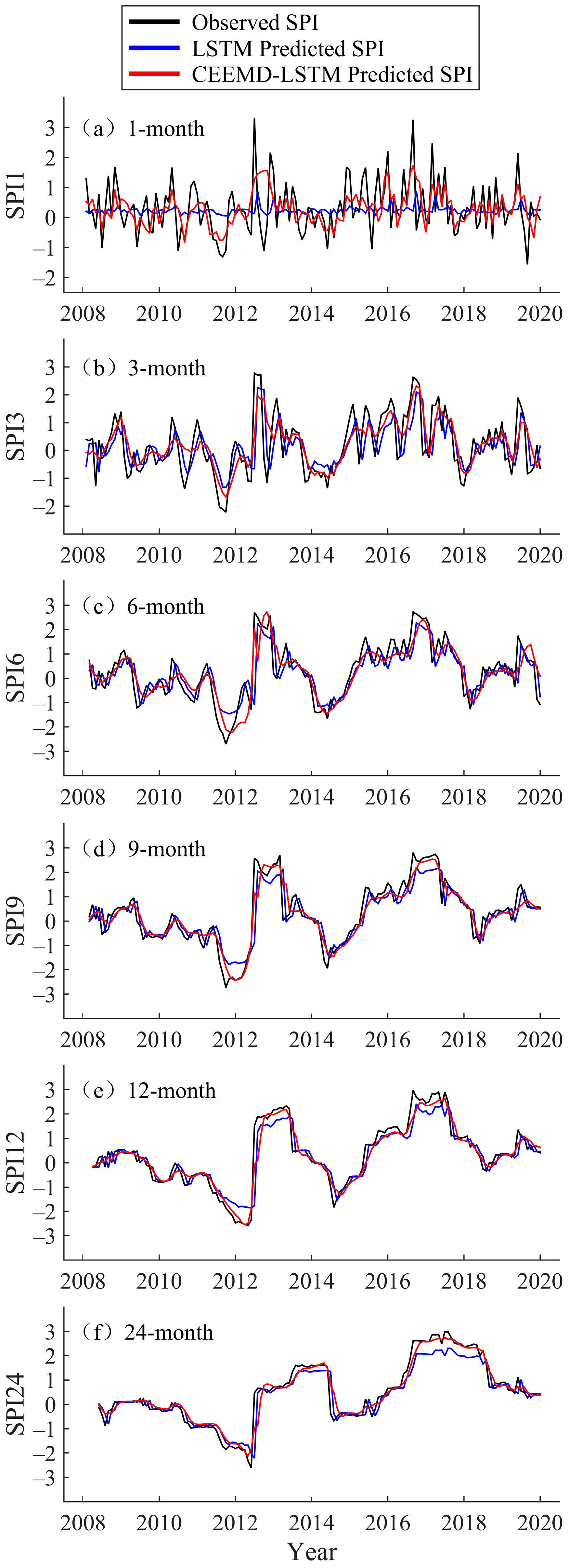
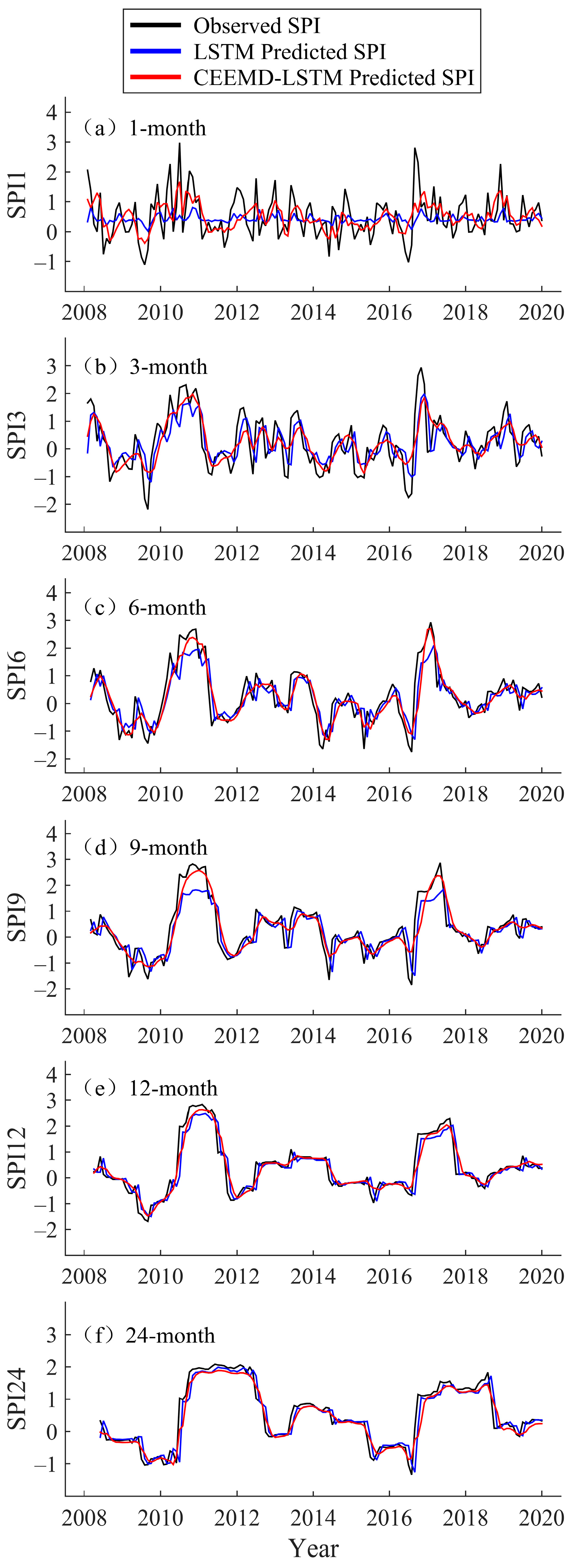
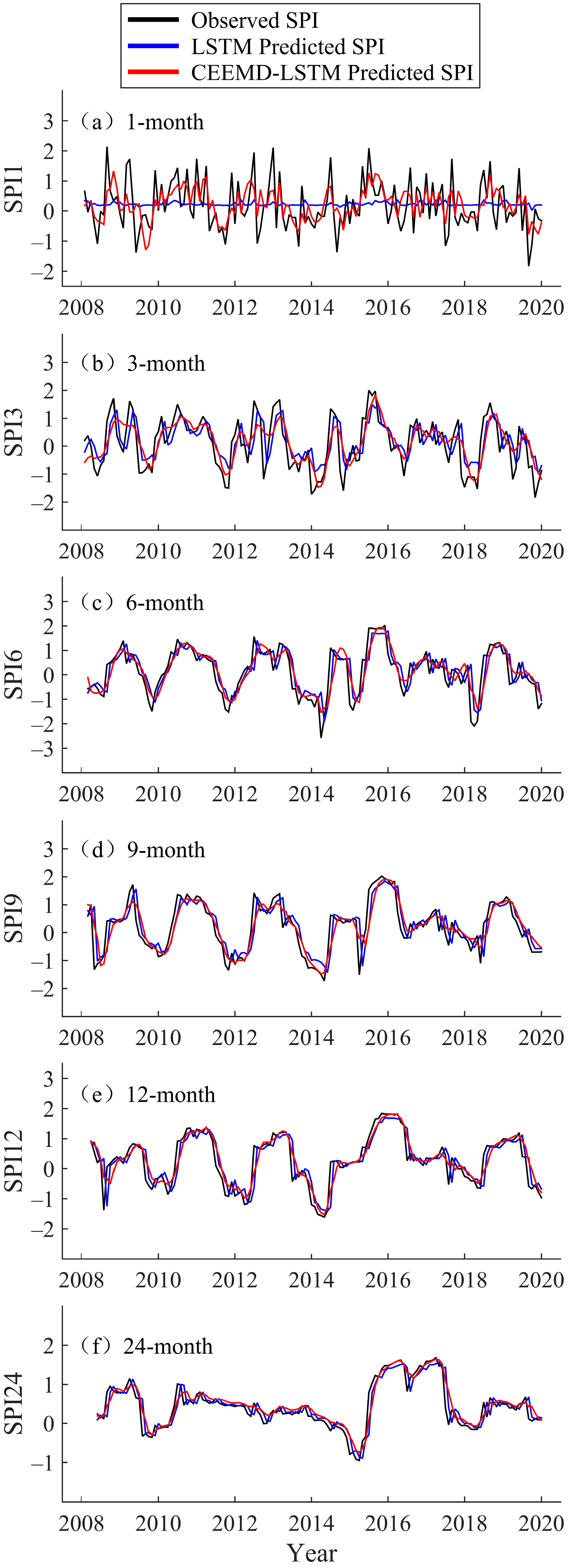
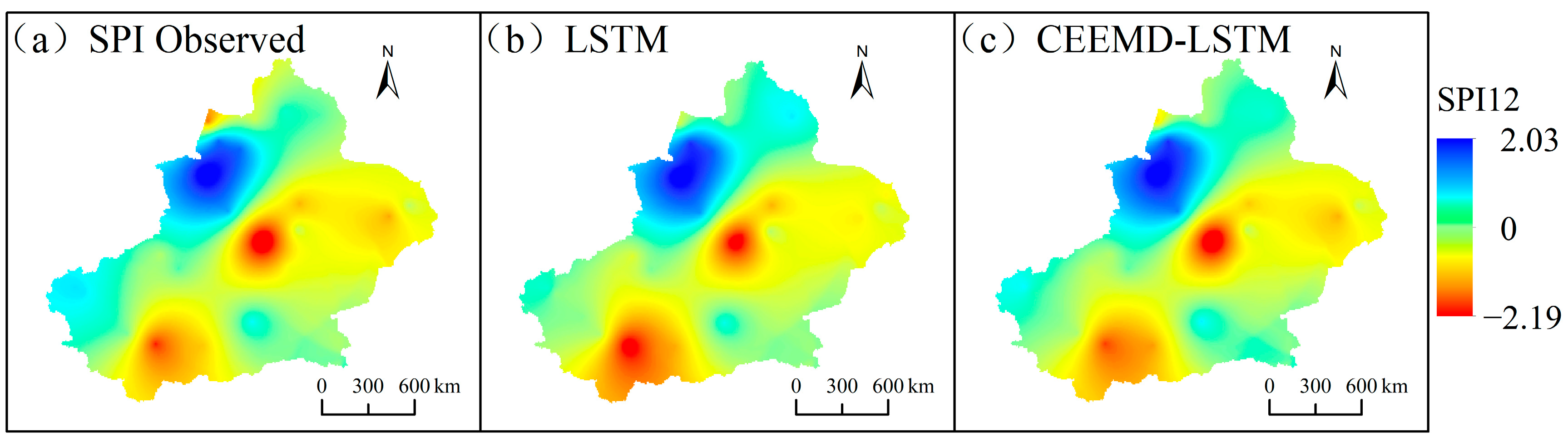
3.3. Hybrid CEEMD-LSTM Model Prediction Results

The data from 1960 to 2007 were used as the training data. Therefore, only this part of the dataset was decomposed by CEEMD. After several modifications and comparisons of the parameters, the standard deviation of the original time-series was finally set to 0.2, the Gaussian white noise logarithm was 100, and the total number of modes (not including the trend) was 8. The multi-scale SPI was decomposed by CEEMD, and eight IMF components and one trend item were obtained. Taking the decomposition of SPI3 at Hami station as an example, the original sequence and the decomposed subsequence are shown in Figure 9. As can be seen in Figure 9, the fluctuation range of the original series is large, while that of the decomposed IMF components is small. Additionally, the fluctuations of the components tend to be smooth as the decomposition proceeds gradually. It is shown that after CEEMD decomposition, the original sequence with strong fluctuations can be decomposed into a set of IMF components with lower fluctuations, which improves the predictability of the sequence.
In the testing phase, the hybrid CEEMD-LSTM model was used to predict the data from 2008 to 2019, and the prediction results for Fuhai, Kuerle, Yutian, and Hami station are shown in Figure 5, Figure 6, Figure 7 and Figure 8, respectively. For all four stations, there is a significant difference between the LSTM predicted value and the observed SPI value at the 1-month timescale. In particular, the LSTM seems to lose its learning ability when forecasting SPI1 at Hami station (Figure 8). At SPI3, SPI6, SPI9, SPI12, and SPI24, the difference between the LSTM predicted and observed value is reduced. In this study, the data volume at SPI1 was the largest and the time-series was the least smooth, thus, the prediction was most ineffective at that timescale. The SPI time-series is a non-stationary series, but the accuracy of the single model prediction results is strongly influenced by the stationarity of the original data. Similarly, Adikari et al. [39] predicted the SPI using LSTM, and it provided only merely acceptable results at Nonghine, Sekong River Basin.
The predicted value of the hybrid CEEMD-LSTM model is closer to the observed SPI, and the predicted SPI trend is consistent with the actual trend. In Figure 5, Figure 6, Figure 7 and Figure 8, the hybrid model performs well at SPI6, SPI9, SPI12, and SPI24. As can be seen from Figure 6, an extreme drought occurred in the Xinjiang Uygur Autonomous Region in 2011. For this year, the hybrid model’s prediction of drought conditions was more consistent with the actual situation and it more accurately predicted the occurrence of extreme drought. Through CEEMD decomposition, local features of the original series at different scales are extracted, and the non-stationary time-series are transformed into stationary components. This reduces the non-stationarity of SPI sequences, which improves the ability of LSTM to predict SPI sequences. Therefore, the hybrid CEEMD-LSTM model has a good performance, even in forecasting SPI1 at each station.
With an increasing timescale, the accuracy of the predictions of the LSTM and CEEMD-LSTM models improves. At the 24-month scale, the prediction results of both models are nearly consistent with the observed SPI. Since the prediction accuracy of the single model gradually improves, that of the hybrid model also improves. At SPI1, the prediction of the hybrid CEEMD-LSTM model is significantly better than that of the single model because the predictability of the subseries, which are obtained from the CEEMD decomposition, is higher than that of the original series. However, this advantage of the combined model diminishes with an increasing timescale. At SPI12 and SPI24, the CEEMD-LSTM model only slightly outperforms the single model. The reason for this is that the long timescale SPI series aggregates more information from the original data and the whole series tends to be stable. Therefore, the prediction accuracy of the single model is improved. In recent years, several scholars have used hybrid models for forecasting. They have found that the results of hybrid models, especially those combining decomposition methods with forecasting methods, are better than those of single models [22,27,40,41,42]. The difference between the aforementioned studies and the current study is that the current study uses such a hybrid model in drought prediction, and the decomposition method chosen was CEEMD. CEEMD is more suitable for prediction because it can effectively solve the problem of mode aliasing and reduce the residual white noise.
The accuracy of the predicted values of the LSTM and CEEMD-LSTM models was evaluated using the Kruskal–Wallis test. The results showed that the p-values of the predicted sequences were greater than 0.05, except for the LSTM predicted SPI1 values at Fuhai station (0.015) and Hami station (0.003). This means that the differences between the observed values and the predicted values of the hybrid CEEMD-LSTM model is not statistically significant, and the CEEMD-LSTM model is able to predict all timescales at different sites, while the LSTM model may not be proficient in predicting the most unstable SPI1 sequences. Four evaluation metrics, namely MAE, RMSE, NSE, and WI, were used to evaluate the prediction results of the two models (Table 3). At the four stations, the MAE values of LSTM were above 0.5 at SPI1, and were mostly below 0.2 at SPI24. The MAE value tends to decrease with an increasing timescale, and RMSE displays the same, while NSE and WI display the opposite trend. These trends indicate that the prediction accuracy of LSTM constantly improves with an increasing timescale. The hybrid CEEMD-LSTM model outperforms the LSTM model in prediction at different timescales, which means that CEEMD can effectively improve the prediction accuracy of the LSTM model. At SPI24, the NSE values of the hybrid model for the four sites were 0.895, 0.930, 0.908, and 0.852, respectively, and the WI values were all above 0.95.
As seen in Figure 6, extreme drought has occurred in the Xinjiang Uygur Autonomous Region during the past 10 years, specifically in 2011. The LSTM and CEEMD-LSTM model prediction results of 32 meteorological stations in 2011 were visualized by the Empirical Bayesian Kriging (EBK) in ArcGIS, as shown in Figure 10. From the figure, we can see that the prediction of the hybrid CEEMD-LSTM model for the spatial distribution of drought is closest to the actual situation. Based on the advantage of CEEMD in non-stationary signal processing, the hybrid model has better performance in SPI prediction.

4. Conclusions

In this study, the LSTM and CEEMD-LSTM models were used to forecast SPI at six timescales in the Xinjiang Uygur Autonomous Region, China. Four statistical criteria were selected to evaluate the prediction accuracy of the two models, and the spatial distribution of the prediction results of the LSTM and CEEMD-LSTM models were visualized using the EBK method.
Based on the values of the statistical criteria (Table 3), the performance of both models increased gradually with increasing timescale. They were lowest at the 1-month scale and highest at the 24-month scale. Moreover, the prediction accuracy of the hybrid model was higher than that of the single model at different timescales. At SPI24, the NSE values of the hybrid model were all greater than 0.85, which shows that CEEMD has advantages in dealing with non-stationary and non-linear data. Through CEEMD decomposition, the original time sequence becomes stable and the predictability of the sequence is improved. Based on Figure 10, we can see that the spatial distribution of drought predicted by the hybrid CEEMD-LSTM model is more consistent with the actual situation. As the prediction accuracy of the hybrid model is better than that of the single model at each timescale, the hybrid model composed of CEEMD and LSTM can contribute to improving the prediction accuracy of meteorological drought.
There are some limitations to this study. In this study, the SPI was chosen to reflect the drought conditions based on its multi-timescale application characteristics and can be calculated by precipitation alone. However, in recent years, both the precipitation and temperature in the Xinjiang Uygur Autonomous Region have shown an increasing trend, and thus the drought characteristics cannot be fully reflected by precipitation. In the subsequent study on the applicability of the combined model, the prediction of several drought indices, such as the SPEI, should be considered.

Author Contributions

Conceptualization, Y.D.; methodology, Y.D.; software, G.Y.; validation, R.T. and G.Y.; data curation, Y.S.; writing—original draft, Y.D.; writing—review and editing, Y.S.; visualization, G.Y.; supervision, Y.S.; project administration, Y.S. All authors have read and agreed to the published version of the manuscript.

Funding

This research was funded by the National Natural Science Foundation of China (No. 41671392, No. 41871297).

Institutional Review Board Statement

Not applicable.

Informed Consent Statement

Not applicable.

Data Availability Statement

The datasets are available from the National Meteorological Data Center (http://data.cma.cn/ accessed on 13 March 2020).

Conflicts of Interest

The authors declare no conflict of interest.

Nomenclature

SPIstandardized precipitation index
SPEIstandardized precipitation evapotranspiration index
RDIreconnaissance drought index
PDSIPalmer drought severity index
EMDempirical mode decomposition
EEMDensemble empirical mode decomposition
CEEMDcomplementary ensemble empirical mode decomposition
ARMAautoregressive and moving average
ANNsartificial neural networks
RNNsrecurrent neural networks
LSTMlong short-term memory
NSENash–Sutcliffe efficiency
WIWillmott index
RMSEroot mean square error
MAEmean absolute error
MSEmean squared error

References

  1. Fan, X.; Miao, C.; Duan, Q.; Shen, C.; Wu, Y. Future Climate Change Hotspots Under Different 21st Century Warming Scenarios. Earths Future 2021, 9, e2021EF002027. [Google Scholar] [CrossRef]
  2. Sun, Q.; Miao, C.; Hanel, M.; Borthwick, A.G.L.; Duan, Q.; Ji, D.; Li, H. Global Heat Stress on Health, Wildfires, and Agricultural Crops under Different Levels of Climate Warming. Environ. Int. 2019, 128, 125–136. [Google Scholar] [CrossRef] [PubMed]
  3. Cai, S.; Song, X.; Hu, R.; Leng, P.; Li, X.; Guo, D.; Zhang, Y.; Hao, Y.; Wang, Y. Spatiotemporal Characteristics of Agricultural Droughts Based on Soil Moisture Data in Inner Mongolia from 1981 to 2019. J. Hydrol. 2021, 603, 127104. [Google Scholar] [CrossRef]
  4. Dai, M.; Huang, S.; Huang, Q.; Zheng, X.; Su, X.; Leng, G.; Li, Z.; Guo, Y.; Fang, W.; Liu, Y. Propagation Characteristics and Mechanism from Meteorological to Agricultural Drought in Various Seasons. J. Hydrol. 2022, 610, 127897. [Google Scholar] [CrossRef]
  5. Shi, M.; Yuan, Z.; Shi, X.; Li, M.; Chen, F.; Li, Y. Drought Assessment of Terrestrial Ecosystems in the Yangtze River Basin, China. J. Clean. Prod. 2022, 362, 132234. [Google Scholar] [CrossRef]
  6. Wang, S.; Li, R.; Wu, Y.; Zhao, S. Effects of Multi-Temporal Scale Drought on Vegetation Dynamics in Inner Mongolia from 1982 to 2015, China. Ecol. Indic. 2022, 136, 108666. [Google Scholar] [CrossRef]
  7. Ortega-Gómez, T.; Pérez-Martín, M.A.; Estrela, T. Improvement of the Drought Indicators System in the Júcar River Basin, Spain. Sci. Total Environ. 2018, 610–611, 276–290. [Google Scholar] [CrossRef]
  8. Sivakumar, V.L.; Ramalakshmi, M.; Krishnappa, R.R.; Manimaran, J.C.; Paranthaman, P.K.; Priyadharshini, B.; Periyasami, R.K. An Integration of Geospatial Technology and Standard Precipitation Index (SPI) for Drought Vulnerability Assessment for a Part of Namakkal District, South India. Mater. Today Proc. 2020, 33, 1206–1211. [Google Scholar]
  9. Zhang, Y.; Li, W.; Chen, Q.; Pu, X.; Xiang, L. Multi-Models for SPI Drought Forecasting in the North of Haihe River Basin, China. Stoch. Environ. Res. Risk Assess. 2017, 31, 2471–2481. [Google Scholar] [CrossRef]
  10. Bera, B.; Shit, P.K.; Sengupta, N.; Saha, S.; Bhattacharjee, S. Trends and Variability of Drought in the Extended Part of Chhota Nagpur Plateau (Singbhum Protocontinent), India Applying SPI and SPEI Indices. Environ. Chall. 2021, 5, 100310. [Google Scholar] [CrossRef]
  11. Dikshit, A.; Pradhan, B.; Huete, A. An Improved SPEI Drought Forecasting Approach Using the Long Short-Term Memory Neural Network. J. Environ. Manag. 2021, 283, 111979. [Google Scholar] [CrossRef] [PubMed]
  12. Musei, S.K.; Nyaga, J.M.; Dubow, A.Z. SPEI-Based Spatial and Temporal Evaluation of Drought in Somalia. J. Arid. Environ. 2021, 184, 104296. [Google Scholar] [CrossRef]
  13. Wang, Z.; Yang, Y.; Zhang, C.; Guo, H.; Hou, Y. Historical and Future Palmer Drought Severity Index with Improved Hydrological Modeling. J. Hydrol. 2022, 610, 127941. [Google Scholar] [CrossRef]
  14. Zhang, J.; Sun, F.; Lai, W.; Lim, W.H.; Liu, W.; Wang, T.; Wang, P. Attributing Changes in Future Extreme Droughts Based on PDSI in China. J. Hydrol. 2019, 573, 607–615. [Google Scholar] [CrossRef]
  15. Asadi Zarch, M.A.; Sivakumar, B.; Sharma, A. Droughts in a Warming Climate: A Global Assessment of Standardized Precipitation Index (SPI) and Reconnaissance Drought Index (RDI). J. Hydrol. 2015, 526, 183–195. [Google Scholar] [CrossRef]
  16. Cheng, Q.; Gao, L.; Zhong, F.; Zuo, X.; Ma, M. Spatiotemporal Variations of Drought in the Yunnan-Guizhou Plateau, Southwest China, during 1960–2013 and Their Association with Large-Scale Circulations and Historical Records. Ecol. Indic. 2020, 112, 106041. [Google Scholar] [CrossRef]
  17. Wu, J.; Chen, X.; Yao, H.; Zhang, D. Multi-Timescale Assessment of Propagation Thresholds from Meteorological to Hydrological Drought. Sci. Total Environ. 2021, 765, 144232. [Google Scholar] [CrossRef]
  18. Xu, Y.; Zhang, X.; Hao, Z.; Singh, V.P.; Hao, F. Characterization of Agricultural Drought Propagation over China Based on Bivariate Probabilistic Quantification. J. Hydrol. 2021, 598, 126194. [Google Scholar] [CrossRef]
  19. Seibert, M.; Merz, B.; Apel, H. Seasonal Forecasting of Hydrological Drought in the Limpopo Basin: A Comparison of Statistical Methods. Hydrol. Earth Syst. Sci. 2017, 21, 1611–1629. [Google Scholar] [CrossRef]
  20. Song, Y.H.; Chung, E.S.; Shahid, S. Differences in Extremes and Uncertainties in Future Runoff Simulations Using SWAT and LSTM for SSP Scenarios. Sci. Total Environ. 2022, 838, 156162. [Google Scholar] [CrossRef]
  21. Senanayake, S.; Pradhan, B.; Alamri, A.; Park, H.-J. A New Application of Deep Neural Network (LSTM) and RUSLE Models in Soil Erosion Prediction. Sci. Total Environ. 2022, 845, 157220. [Google Scholar] [CrossRef] [PubMed]
  22. Liu, M.D.; Ding, L.; Bai, Y.L. Application of Hybrid Model Based on Empirical Mode Decomposition, Novel Recurrent Neural Networks and the ARIMA to Wind Speed Prediction. Energy Convers. Manag. 2021, 233, 113917. [Google Scholar] [CrossRef]
  23. Wang, W.C.; Chau, K.W.; Qiu, L.; Chen, Y.B. Improving Forecasting Accuracy of Medium and Long-Term Runoff Using Artificial Neural Network Based on EEMD Decomposition. Environ. Res. 2015, 139, 46–54. [Google Scholar] [CrossRef]
  24. Zhu, S.; Lian, X.; Wei, L.; Che, J.; Shen, X.; Yang, L.; Qiu, X.; Liu, X.; Gao, W.; Ren, X.; et al. PM2.5 Forecasting Using SVR with PSOGSA Algorithm Based on CEEMD, GRNN and GCA Considering Meteorological Factors. Atmos. Environ. 2018, 183, 20–32. [Google Scholar] [CrossRef]
  25. Wang, S.; Zhang, N.; Wu, L.; Wang, Y. Wind Speed Forecasting Based on the Hybrid Ensemble Empirical Mode Decomposition and GA-BP Neural Network Method. Renew. Energy 2016, 94, 629–636. [Google Scholar] [CrossRef]
  26. Bahmani, R.; Ouarda, T.B.M.J. Groundwater Level Modeling with Hybrid Artificial Intelligence Techniques. J. Hydrol. 2021, 595, 125659. [Google Scholar] [CrossRef]
  27. Johny, K.; Pai, M.L.; Adarsh, S. A Multivariate EMD-LSTM Model Aided with Time Dependent Intrinsic Cross-Correlation for Monthly Rainfall Prediction. Appl. Soft Comput. 2022, 123, 108941. [Google Scholar] [CrossRef]
  28. Mckee, T.B.; Doesken, N.J.; Kleist, J. The relationship of drought frequency and duration to time scales. In Proceedings of the 8th Conference on Applied Climatology, Anaheim, CA, USA, 17–22 January 1993; pp. 179–184. [Google Scholar]
  29. Svoboda, M.; Hayes, M.; Wood, D. Standardized Precipitation Index User Guide; WMO-No. 1090; World Meteorological Organization (WMO): Geneva, Switzerland, 2012. [Google Scholar]
  30. Huang, Y.F.; Ang, J.T.; Tiong, Y.J.; Mirzaei, M.; Amin, M.Z.M. Drought Forecasting Using SPI and EDI under RCP-8.5 Climate Change Scenarios for Langat River Basin, Malaysia. Procedia Eng. 2016, 154, 710–717. [Google Scholar] [CrossRef]
  31. Tsakiris, G.; Vangelis, H. Towards a Drought Watch System Based on Spatial SPI. Water Resour. Manag. 2004, 18, 1–12. [Google Scholar] [CrossRef]
  32. Yerdelen, C.; Abdelkader, M.; Eris, E. Assessment of Drought in SPI Series Using Continuous Wavelet Analysis for Gediz Basin, Turkey. Atmos. Res. 2021, 260, 105687. [Google Scholar] [CrossRef]
  33. Javed, T.; Li, Y.; Rashid, S.; Li, F.; Hu, Q.; Feng, H.; Chen, X.; Ahmad, S.; Liu, F.; Pulatov, B. Performance and Relationship of Four Different Agricultural Drought Indices for Drought Monitoring in China’s Mainland Using Remote Sensing Data. Sci. Total Environ. 2021, 759, 143530. [Google Scholar] [CrossRef] [PubMed]
  34. Yeh, J.R.; Shieh, J.S.; Huang, N.E. Complementary Ensemble Empirical Mode Decomposition: A Novel Noise Enhanced Data Analysis Method. Adv. Adapt. Data Anal. 2010, 2, 135–156. [Google Scholar] [CrossRef]
  35. Hochreiter, S.; Schmidhuber, J. Long Short-Term Memory. Neural Comput. 1997, 9, 1735–1780. [Google Scholar] [CrossRef] [PubMed]
  36. Ko, M.S.; Lee, K.; Kim, J.K.; Hong, C.W.; Dong, Z.Y.; Hur, K. Deep Concatenated Residual Network with Bidirectional LSTM for One-Hour-Ahead Wind Power Forecasting. IEEE Trans. Sustain. Energy 2021, 12, 1321–1335. [Google Scholar] [CrossRef]
  37. Vijayaprabakaran, K.; Sathiyamurthy, K. Towards Activation Function Search for Long Short-Term Model Network: A Differential Evolution Based Approach. J. King Saud Univ.-Comput. Inf. Sci. 2020, 34, 2637–2650. [Google Scholar] [CrossRef]
  38. Weiss Technion, G.; Goldberg, I.Y.; Yahav, E. On the Practical Computational Power of Finite Precision RNNs for Language Recognition. In Proceedings of the 56th Annual Meeting of the Association for Computational Linguistics (Short Papers), Melbourne, Australia, 15–20 July 2018; pp. 740–745. [Google Scholar]
  39. Adikari, K.E.; Shrestha, S.; Ratnayake, D.T.; Budhathoki, A.; Mohanasundaram, S.; Dailey, M.N. Evaluation of Artificial Intelligence Models for Flood and Drought Forecasting in Arid and Tropical Regions. Environ. Model. Softw. 2021, 144, 105136. [Google Scholar] [CrossRef]
  40. Chen, X.; Li, F.W.; Feng, P. A New Hybrid Model for Nonlinear and Non-Stationary Runoff Prediction at Annual and Monthly Time Scales. J. Hydro-Environ. Res. 2018, 20, 77–92. [Google Scholar] [CrossRef]
  41. Feng, Z.K.; Niu, W.J.; Tang, Z.Y.; Jiang, Z.Q.; Xu, Y.; Liu, Y.; Zhang, H.R. Monthly Runoff Time Series Prediction by Variational Mode Decomposition and Support Vector Machine Based on Quantum-Behaved Particle Swarm Optimization. J. Hydrol. 2020, 583, 124627. [Google Scholar] [CrossRef]
  42. Wen, X.; Feng, Q.; Deo, R.C.; Wu, M.; Yin, Z.; Yang, L.; Singh, V.P. Two-Phase Extreme Learning Machines Integrated with the Complete Ensemble Empirical Mode Decomposition with Adaptive Noise Algorithm for Multi-Scale Runoff Prediction Problems. J. Hydrol. 2019, 570, 167–184. [Google Scholar] [CrossRef]
Figure 1. Geographical information and meteorological station distribution in Xinjiang Uygur Autonomous Region.
Atmosphere 13 01504 g001
Figure 2. Structure diagram of long short-term memory.
Atmosphere 13 01504 g002
Figure 3. Workflow of the CEEMD-LSTM combined model.
Atmosphere 13 01504 g003
Figure 4. Observed SPI values at the 1-, 3-, 6-, 9-, 12-, and 24-month timescales of the example stations.
Atmosphere 13 01504 g004
Figure 5. Forecast of multi-timescale SPI values of the LSTM and CEEMD-LSTM model at Fuhai Station (2008–2019).
Atmosphere 13 01504 g005
Figure 6. Forecast of multi-timescale SPI values of the LSTM and CEEMD-LSTM model at Kuerle Station (2008–2019).
Atmosphere 13 01504 g006
Figure 7. Forecast of multi-timescale SPI values of the LSTM and CEEMD-LSTM model at Yutian Station (2008–2019).
Atmosphere 13 01504 g007
Figure 8. Forecast of multi-timescale SPI values of the LSTM and CEEMD-LSTM model at Hami Station (2008–2019).
Atmosphere 13 01504 g008
Figure 9. The CEEMD decomposition results of SPI3 sequence.
Atmosphere 13 01504 g009
Figure 10. Spatial distributions of SPI in 2011, using LSTM and CEEMD-LSTM model.
Atmosphere 13 01504 g010
Table 1. Drought classification based on standardized precipitation index.
SPI ValueClassification
−0.5+No drought
−0.5 to −0.99Mild drought
−1.0 to −1.49Moderate drought
−1.5 to −1.99 Severe drought
−2.0 and lessExtreme drought
Table 2. Mann–Kendall trend test for SPI sequences.
Example StationsSPI Seriesp ValueTrend
FuhaiSPI12.492 × 10−5increasing
SPI33.721 × 10−10increasing
SPI68.860 × 10−14increasing
SPI91.665 × 10−14increasing
SPI122.220 × 10−16increasing
SPI240.000increasing
KuerleSPI10.081no trend
SPI30.001increasing
SPI63.329 × 10−5increasing
SPI96.254 × 10−6increasing
SPI128.926 × 10−7increasing
SPI244.159 × 10−12increasing
YutianSPI10.035increasing
SPI30.001increasing
SPI61.649 × 10−4increasing
SPI92.321 × 10−4increasing
SPI124.652 × 10−4increasing
SPI241.990 × 10−11increasing
HamiSPI10.006increasing
SPI39.700 × 10−7increasing
SPI63.212 × 10−12increasing
SPI91.332 × 10−15increasing
SPI120.000increasing
SPI240.000increasing
Table 3. Comparison of the observed and predicted values of the two models using statistical criteria.
Example StationsSPI SeriesModelMAERMSENSEWI
FuhaiSPI1LSTM0.7901.028−32.3710.255
CEEMD-LSTM0.6750.815−0.6330.721
SPI3LSTM0.5510.681−0.1120.781
CEEMD-LSTM0.4740.5780.2470.850
SPI6LSTM0.3890.4910.4980.885
CEEMD-LSTM0.2950.3780.7140.934
SPI9LSTM0.2750.3600.6820.924
CEEMD-LSTM0.2190.2910.7900.951
SPI12LSTM0.2190.2940.7730.946
CEEMD-LSTM0.1690.2190.8730.970
SPI24LSTM0.1520.1980.8360.960
CEEMD-LSTM0.1190.1520.8950.976
KuerleSPI1LSTM0.6480.868−46.2800.168
CEEMD-LSTM0.5680.739−0.9040.688
SPI3LSTM0.6040.791−0.2170.778
CEEMD-LSTM0.5020.6740.2140.850
SPI6LSTM0.4710.6600.4510.890
CEEMD-LSTM0.4120.5400.7170.934
SPI9LSTM0.3860.5730.6700.933
CEEMD-LSTM0.2840.4080.8660.969
SPI12LSTM0.3080.4860.7940.957
CEEMD-LSTM0.2250.3420.9150.981
SPI24LSTM0.2700.4270.8420.967
CEEMD-LSTM0.1960.3120.9300.984
YutianSPI1LSTM0.5410.711−28.5230.307
CEEMD-LSTM0.5090.615−1.2570.678
SPI3LSTM0.5250.692−0.1840.796
CEEMD-LSTM0.4860.6120.1170.842
SPI6LSTM0.4190.5600.4450.889
CEEMD-LSTM0.3240.4390.7400.942
SPI9LSTM0.3680.5410.5130.903
CEEMD-LSTM0.2960.4180.7770.949
SPI12LSTM0.2390.3930.8050.956
CEEMD-LSTM0.1960.3000.8890.975
SPI24LSTM0.1780.3230.8630.967
CEEMD-LSTM0.1770.2600.9080.979
HamiSPI1LSTM0.6610.806−194.8850.115
CEEMD-LSTM0.5170.650−0.6140.724
SPI3LSTM0.5320.673−0.2080.787
CEEMD-LSTM0.4700.5830.2310.851
SPI6LSTM0.3970.5740.4790.884
CEEMD-LSTM0.3520.4660.6540.924
SPI9LSTM0.3420.5010.5780.904
CEEMD-LSTM0.2860.4060.7220.937
SPI12LSTM0.2630.4200.6870.925
CEEMD-LSTM0.2160.3150.8190.958
SPI24LSTM0.1590.2440.7900.950
CEEMD-LSTM0.1390.2010.8520.966
Publisher’s Note: MDPI stays neutral with regard to jurisdictional claims in published maps and institutional affiliations.

