Article

Parameterization of a Rising Smoke Plume for a Large Moving Ship Based on CFD

1
Department of Environmental Science and Engineering, Fudan University, Shanghai 200433, China
2
Zhejiang Marine Ecology and Environment Monitoring Center, Zhoushan 316021, China
3
Shanghai Key Laboratory of Atmospheric Particle Pollution and Prevention (LAP3), Fudan University, Shanghai 200433, China
4
Institute of Eco-Chongming (IEC), No. 3663 Northern Zhongshan Road, Shanghai 200062, China
*
Author to whom correspondence should be addressed.
Atmosphere 2022, 13(9), 1507; https://doi.org/10.3390/atmos13091507
Submission received: 14 July 2022 / Revised: 3 September 2022 / Accepted: 10 September 2022 / Published: 15 September 2022
(This article belongs to the Section Air Quality)

Abstract

:
The plume rising height of a ship will directly affect the maximum ground concentration and distance from the source caused by flue gas emission. Ship movement has an important effect on plume rising, but it is often ignored in previous studies. We simulated the weakening effect caused by ship movement by considering the influence of four main parameters (wind speed, ship speed, flue gas exit velocity, and flue gas exit temperature) on the smoke plume rising height, using the computational fluid dynamics (CFD) model (PHOENICS version 6.0 CHAM, London, UK). The main parameters affecting the difference in plume rising height between stationary and moving sources for the same parameter settings are the wind speed and the ship speed. Therefore, we established two simplified calculation methods that corrected the flue gas exit velocity ( V e x i t ) and the flue gas exit temperature ( T ) for approximately simulating the smoke plume rising height of the moving ship using the formula of a stationary ship. Verification cases indicated that the corrected V e x i t   (the average of relative error is 5.48%) and the corrected T (the average of relative error is 60.07%) not only saved calculation time but also improved the simulation accuracy compared with the uncorrected stationary source scheme (the average of relative error is 135.38%). Of these correction methods, the scheme with corrected V e x i t is more effective. The intention is to provide some references for the field experimentation of moving ship plume rising in different ports in the future and to further study the mechanism of moving ship plume rising.

1. Introduction

Emissions from ships are increasing year by year and will increase in the future due to the growth in global trade. Air pollutant emissions from ships entering and leaving ports greatly affect the air quality in coastal areas [1,2,3] and inland areas hundreds of kilometers away [4]. Air pollutants also contribute to global atmospheric changes [5,6]. Ship emission pollutants range from conventional air pollutants, such as SO2 [7], NOX [8], and PM [9,10], to organic pollutants [11] and some secondary inorganic ions [12]. These pollutants not only affect air quality directly but also pose a significant potential health risk [13,14,15,16], causing a certain number of premature deaths each year. It is therefore very important to study the dispersion of air pollutants emitted from ships to update the standards of air pollutants emitted from ships and to improve the air quality in the port areas in order to ultimately facilitate sustainable growth [17].
Model simulations are used to study the dispersion of ship exhaust plumes [18]. Models such as the weather research and forecasting with chemistry (WRF/Chem) model [19,20], the weather research and forecasting community multiscale air quality (WRF/CMAQ) model [21], and the California puff (CALPUFF) model [22,23,24,25], can obtain good simulation results. In these previous studies, ship pollution is often generalized as a non-point source to simulate its diffusion, and in the process of ship movement, moving pollution sources are often generalized as fixed line sources, which may cause some errors in the detection of ship pollutant concentration at port scale. Using the CALPUFF model as an example, the CALPUFF model is a three-dimensional unsteady air quality model developed on the basis of the Lagrange smoke cluster model. Based on similarity equation, turbulence, emission strengths, transformation, and removal, the CALPUFF model uses space and time varying meteorology to model gas and particle diffusion, considering buoyancy and momentum plume rise, stack effect, and building effect. It can simulate the transport of pollutants over a distance of 50 km and above, and has good simulation results for the diffusion of point sources, line sources, and unsteady conditions (quiet wind, smoke, coastal effect, etc.) [16]. A short-term field experiment was conducted at Yantian Port in Shenzhen, China in June 2018. The experimental results, however, show that the air pollutant concentration simulated by CALPUFF was lower than that observed on the shore. This underestimation may be related to the low estimation of ship source intensity or the failure of the simulations to account for emissions from gathering and transporting machinery in the port area. Some ship emission simulation studies also underestimated the actual concentrations of air pollutants [26,27]. The underestimation rate was related to the ratio of gas velocity to wind speed at funnel height (UR). The UR increased and the underestimation rate decreased. This was because an increase in UR means an increase in the pollutant momentum flux, which enhances the plume ascending effect and weakens the plume diffusion effect. The rise of the ship plume will therefore be affected by the flue gas exit velocity and wind speed.
The general underestimation mentioned focused attention on the ship exhaust pollution source characteristics. We speculated that this may be due to the fact that the simulated effective source height is much higher than the actual plume height, which may be related to the layout of the ship chimneys and the ship’s movements. Xu et al. [28] analyzed the influence of the ship chimney layout. Our study will consider the influence of ship movement on emission plumes dispersion. Plume rising is one of the important behaviors of plume dispersion, which directly affects the maximum ground concentration and distance from the source caused by flue gas emission. Our study, therefore, focuses on the influence of ship movement on plume rising height.
Plume rising is caused by two factors: dynamic uplift and buoyancy uplift [29]. Dynamic uplift means that the plume has upward kinetic energy, and will still be able to move after leaving the chimney. Buoyancy uplift refers to the density difference caused by the temperature difference, so that the atmosphere, other than the flue gas, produces a buoyancy effect on the flue gas. In the initial stage of plume rising, dynamic uplift is the main factor. With the flue gas mixing with the surrounding atmosphere gradually, the rising speed caused by the initial momentum gradually decreases and the buoyancy uplift starts to play a major role. After that, the turbulence causes the structure of the plume to collapse, and the plume gradually flattens until it no longer rose. Marine flue gas is a high-temperature flue gas, where the combustion exhaust of marine diesel engines contains mainly nitrogen, sulfur oxides, and other gases. The ship exhaust temperature must also be above the acid dew point of the flue gas (generally above 200 °C) to reduce corrosion. To avoid downwash of the flue gas stream, there is also a lower velocity limit on the flue gas exit velocity, where the ratio of the flue gas exit velocity to the wind speed is greater than 2 to inhibit downwash [30]. In the case of high temperatures and certain flue gas exit velocities, the ship emissions are a buoyant moving source [31]. With the gradual release of waste heat from the actual ship plume along the route, the ship’s movement disperses the air mass rather than causing a fixed release of heat, as in the case of a buoyant stationary source. If the plume rising is modeled using a Briggs lift equation that is similar to that in the CALPUFF model, where the source is equivalent to a row of buoyant point sources, enhanced plume rising will be observed due to point source clustering, which will likely cause high modeled plume rising heights. The actual thermal rising of the ship source is however lower, and the plume rising from the moving line source of the ship should be attenuated compared to the point source plume rising, because the duration of the emission at a specific location is short. This indicates that ship movement is not negligible for plume rising, because it can reflect the emission characteristics of the ship as a source of buoyancy movement.
Computational fluid dynamics (CFD) models use finite difference and finite volume methods to solve the Navier–Stokes equations in 3D space, providing complex analyses of fluid flows based on the conservation of mass and momentum [32]. The CFD model can perform more refined modeling of ports and ships, and can well simulate the influence of the hull itself on the flow field due to refined simulation. It is therefore one of the more commonly used methods in environmental pollution research and ship design research. In ship design research, it is used to simulate the flow field of ships and compares well with the actual measurement results [33,34,35]. The CFD model also simulates atmospheric convection conditions that take into account dynamic and thermal effects [36]. In addition, it can also simulate ship emission data with higher temporal resolution and reduce the uncertainty caused by ignoring the hourly fluctuations of ship emissions [37] in coastal urban areas and ports where ship activities are frequent. These applications convinced the authors that rising smoke plumes during ship movement could also be simulated by using the CFD software PHOENICS version 6.0 in this study. This study adopted the CFD model of ship buoyancy source as established by Xu et al. [28]. The ship movement was considered on this basis. The main parameters that affect rising smoke plumes from ships include ship speed, wind speed, flue gas exit velocity, and flue gas exit temperature [28,38,39,40,41,42,43,44]. Wind direction may also be an important factor. When the direction of ship movement is not consistent with the environmental wind direction, it will affect the direction of plume dispersion. However, this influence is local, because the environmental wind covers the whole simulation area, while the hull movement is only local. Kulkarni et al. [45] considered the yaw angle of the ambient wind relative to the ship’s heading, and turned the ship’s heading and the ambient wind into a “synthetic wind” to consider the influence of the yaw angle. This is a simplified simulation method commonly used to observe whether the plume washing around the chimney will cause smoke damage on the deck. However, such results are inaccurate, because it amplifies the local influence of the ship’s navigation. This may not be the main reason why the simulated concentration in our observation experiment, and references [26] and [27], were lower than the observed concentration. The distance between the shoreline observation point and the chimney in our observation experiment is more than one kilometer, and the actual environmental wind speed, at such a distance away from the ship, is closer to the regional background wind speed when the ship travels upwind. The influence of ship navigation on the actual environmental wind speed at the observation point is much smaller than that near the chimney. Therefore, the low simulated concentration at distant observation points should not be caused entirely by the influence of ship navigation on the environmental flow field. We speculated that the more likely reason is that the lifting force of the exhaust plume decreases during sailing.
In this paper, we used the CFD model to simulate the degree of influence of four parameters, namely wind speed, ship speed, flue gas exit velocity, and flue gas exit temperature, on the plume rising height of ships with moving sources. By analyzing the difference in the plume rising height between the stationary source and the moving source under the same parameter setting, new formulas for calculating the plume rising height, including the ship movement, were established.
Section 2 presents the numerical simulation scheme and its parameter values for the transport and diffusion of the ship’s smoke plume. Section 3 shows the analyses of the rising smoke plume, which was simulated for both the stationary source ship and the moving ship. The simulation results of the moving source ship scheme were analyzed relative to the stationary scheme. The results from this analysis were used to establish simplified correction methods to approximate the smoke plume rising heights of moving ships by the relative changes in the two simulation schemes. Section 4 concludes the study.

2. Methods

2.1. Physical Model and Governing Equations

A typical large container ship at the Yantian Port in Shenzhen was selected as the research sample for modeling in June 2018. Figure 1 shows the ship model, the domain, and the grids in the CFD model.
Equations were set up for the CFD (PHOENICS version 6.0) model after the physical model of the ship was imported into the model. A standard k–ε turbulence model, which is a two-equation model, was chosen for the simulation. The differential model was chosen as a hybrid model that combines the central differencing scheme with the first-order upwind. It applies the central differencing scheme when | P e | < 2 and applies the first-order upwind when | P e | 2 , where P e is the Peclet number, indicating the ratio of convective velocity to diffusive velocity. The Boussinesq assumption was also introduced, which is about the density being constant (incompressible flow), allowing only for change due to temperature variations (which induces buoyancy).
Xu et al. [28] validated the above model using wind tunnel experimental data from the literature. The simulation results agree well with the wind tunnel test results, indicating that using the CFD model for the simulation of ship plume behavior is feasible.

2.2. Experimental Case Simulation Parameter Scheme

This study is a parametric simulation of the plume characteristics of a single moving ship. The parameters that influence the rising plume of a ship include the ship speed, wind speed, flue gas exit velocity, and flue gas exit temperature. For actual ships, the ship speed is closely related to the flue gas exit velocity and flue gas temperature. The reference ship sample research data, however, only had the flue gas exit velocity data that changed with ship speed, but not the flue gas exit temperature data. Only the flue gas exit velocity was therefore associated with the working condition in the parameter setting.
Near-surface wind speed statistics from meteorological stations in the Dapeng Bay sea area of Shenzhen from 2009 to 2018 [46] indicated that the wind speed varied between 1.5 and 15 m/s. We subdivided this wind speed segment further into four segments and took the representative wind speed values of each segment for the numerical simulations in this study. Table 1 shows the detailed values. The ship speed values were referenced to the inbound and outbound ship speeds of a sample of ships in Dapeng Bay, Shenzhen in June 2018 (shown in Table A1 in the Appendix A). The ship speeds that were used varied from 0 to 16 knots. These ship speed segments were also further subdivided into four segments. Table 1 shows the representative ship speed value of each segment of the numerical simulation.
The flue gas exit velocities at the representative ship speeds in Table 1 were taken with reference to the range of variation in actual emission data from a sample of ships at Yantian Port, Dapeng Bay, Shenzhen in June 2018 (shown in Table A2 in the Appendix A). Table 2 shows that the flue gas exit velocities of the ship samples that correspond to the four representative ship speeds varied between 0.26 and 1.26 m/s, 0.46 and 2.35 m/s, 1.94 and 10.37 m/s, as well as 5.01 and 26.15 m/s, respectively. The flue gas exit velocity varies considerably with the ship sample for the same ship speed. The influence of flue gas exit velocity on the plume rising for different ship speeds was analyzed. To understand the differences in the plume characteristics between the different ship samples, three flue gas exit velocities were set up based on the exit velocity sample characteristics for each ship speed. The exit velocities were low, medium, and high, representing low, medium, and high emission samples (which are represented by V1, V2, and V3, respectively). The analysis of the flue gas exit velocity effect on the rising plume only considers the difference in the flue gas exit velocities between ship samples for the same ship speed to avoid duplicate analyses. Table 2 shows the simulated emission velocity scenario settings.
Based on the actual ship sample research results, the flue gas exit temperature of the ship varied between 60 and 400 °C (shown in Table A1 in the Appendix A). Since the flue gas exit temperature of the ship is generally higher than 200 °C to prevent acid corrosion, three cases of 200 °C, 300 °C, and 400 °C were therefore taken for this study (represented by T1, T2, and T3). The ship parameter settings were further considered for the three aforementioned flue gas temperature values (T1, T2, and T3), of which the combinations are shown in Table 2. This resulted in the full emission scenario for the actual simulation.
In both the moving source ship simulation and the stationary source ship simulation schemes, all the simulation parameters are the same, except for the movement of the ship. The stationary source ship simulation schemes will therefore also involve the simulation of the emission conditions at different ship speeds, even though the ship is stationary during the simulation. For the stationary source ship simulation, the ship speed changes during the simulation cause the change in the flue gas exit velocity, and are still treated as an effect of the change in ship speed in the analysis of the results to facilitate comparison with the results of the moving source ship schemes.
The area of high air pollutant concentrations contributed by the ship emissions is mainly concentrated close to the coast [21,47], specifically within 1–2 km from the ship track [48]. The air pollutant plume behavior 1 km behind the ship chimney is of specific interest in this study. The smoke plume rising heights of the maximum plume concentration at the 1 km downwind direction of the ship chimney in the X–Z plane was compared after completing the numerical simulations. The cubic spline interpolation of the meshing concentration given by numerical simulation was used to determine the smoke plume rising height.

2.3. Computational Domains, Boundary Conditions, and Simulation Settings

The computing grid and computing domain vary based on the ship speed (see Table 3). The grid setup mainly takes into account the dispersed simulation requirements of emissions. Given the dispersed nature of emissions, we would like to be able to set up at least one grid that has an outlet so that the actual impact of outlet dispersion can be simulated as finely as possible. The software sets the minimum time step for transient simulation to 1 s, so each outlet continues to discharge for at least 1 s. We actually set the duration of a single outlet to be 2~15 s, where 2 s is the discharge outlet duration at the highest ship speed (14 knots). The distance of 2 s from the ship at this ship speed is 14.392 m, so the grid spacing is 15 m. With smaller grids, the emission duration per grid would need to be less than 1 s, a time step setting that cannot be implemented in the software. In order to facilitate the comparison of the simulation results at various ship speeds, the grid spacing in this study is uniformly set as 15 m, that is, each grid on the ship route has at least one discharge outlet. This study determined the emission parameters for different working conditions based on the ship speed. These emission parameters applied to both the moving and stationary source simulation schemes.
All the surfaces of the computational domain and the ship wall were non-slip boundary conditions. The exponential law wind profile was chosen in the vertical direction as the wind blew from the bow to the stern. The ambient fluid air was at 1 atmosphere pressure and the temperature was 20 °C.
The MOFOR function of PHOENICS was used to simulate the ship’s movement. Transient simulations were used for the moving source ship simulation scheme and steady-state simulations were used for the stationary source simulation scheme. A series of INLET objects located in the path of the ship movement was used to simulate pollutant emissions. The INLET properties were used to set the flue gas exit velocity and flue gas exit temperature. The total simulation time for each moving source ship simulation case was 360 s and the results were taken for the period after the flow field stabilized.

3. Results and Discussion

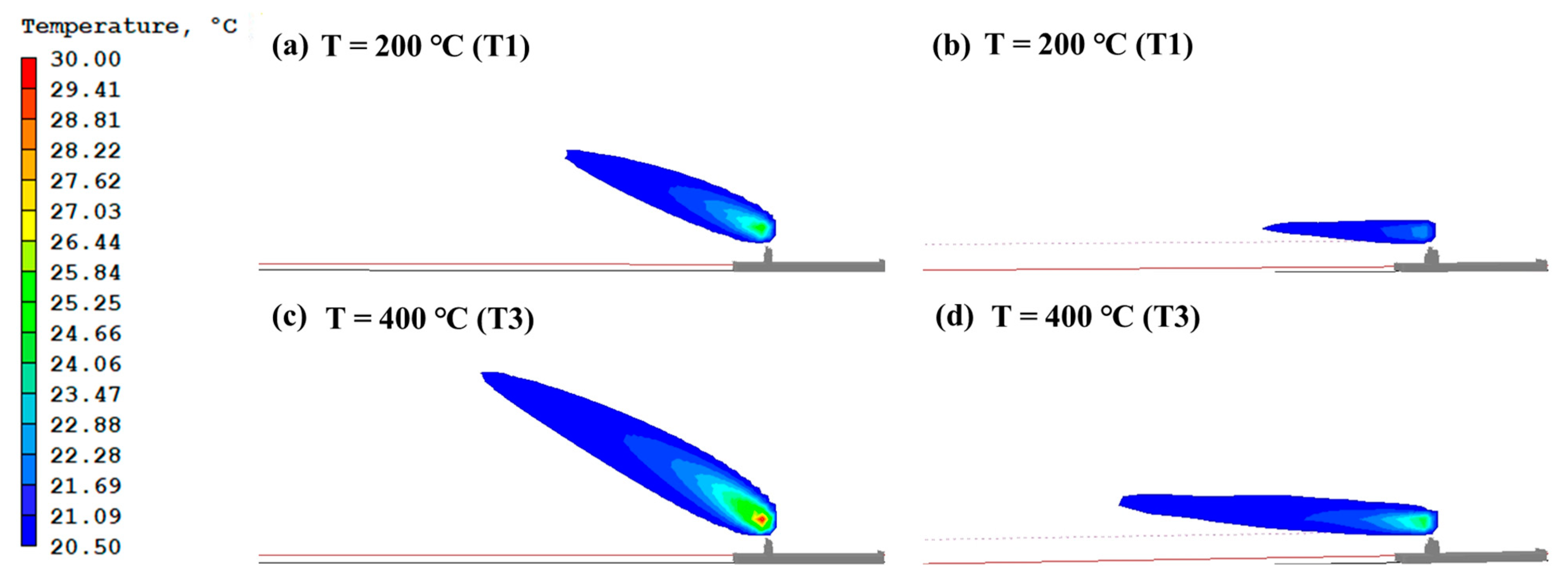
3.1. Rising Height of the Smoke Plume for the Stationary and Moving Source Simulation Schemes

The rising height of the smoke plume of both the stationary source and the moving source schemes varied significantly with wind speed and emission scenarios. Figure 2 shows that the smoke plume rising height (hereafter denoted as H+) of the two schemes always decreases as the wind speed increases from 3 m/s to 12 m/s. This is because as the wind speed of the atmospheric transverse wind gradually increases, the turbulence degree of the flow field intensifies, which accelerates the mixing process of flue gas at the outlet of the chimney and the surrounding atmosphere, and reduces the plume rising height. Emission scenarios also have a significant impact on H+. In Figure 2 for the wind speed of 3 m/s for the S4 group, the H+ gradually increases as the emission levels increase from V1 (5.01 m/s) to V3 (26.15 m/s). Figure 3 shows selected simulation results for the stationary and moving source schemes for different flue gas exit temperatures. At a wind speed of 3 m/s, the H+ increased gradually for both schemes as the flue gas exit temperature increased from T1 (200 °C) to T3 (400 °C) in the S2-V2 group. The reason is that the larger the flue gas exit velocity and temperature, the larger the initial momentum and heat of the flue gas, and the stronger the anti-disturbance ability of the mixed air flow to the transversal wind above the outlet during the process of diffusing into the surrounding atmosphere, leading to the higher plume rising height. The effect of the ship speed on the H+ for the two schemes is, however, significantly different. For the V2 group in Figure 3, the H+ of the stationary source scheme gradually increased with an increase in the ship speed from S1 (2 knots) to S4 (14 knots), as the flue gas exit velocity of S1 is lower than that of S4. The H+ decreased and then increased with the minimum value of H+ at the ship speed S2 scenario (6 knots) for the moving source scheme.
Different parameters affect H+ to different degrees and the same parameter affects H+ to different degrees for different ship source schemes. The relative rate of change (RH+) in H+ with these parameters was therefore calculated for the two modeled schemes (Figure 4). The RH+ was obtained by dividing the difference between the H+ of the simulated and the reference scenario by the H+ of the reference scenario. The H+ of the emission scenario S2-V2-T2 with a wind speed of 3 m/s was used for the reference scenario. The RH+ varied from −100% to 0% for the stationary source scheme and from −90% to 0% for the moving source scheme as the wind speed increased from 3 m/s to 12 m/s. The range of RH+ for the stationary source scheme was approximately −20% to 780% as the ship speed increased from S1 to S4. As described in Section 2.2, the ship is stationary during this simulation and only the change in emission characteristics due to the change in ship speed is simulated. For the moving source scheme, the RH+ varied from 0% to 140%. When the flue gas exit velocity changed from V1 to V3, the range of change in RH+ was approximately −30% to 50% for the stationary source scheme and −60% to 100% for the moving source scheme. With an increase in flue gas exit temperature from T1 to T3, the RH+ varied from −20% to 30% for the stationary source scheme and from −30% to 30% for the moving source scheme. When these parameters are taken together, within their actual range of values, their influence on the H+ of the stationary source simulation scheme is, in descending order, the ship speed, wind speed, flue gas exit velocity, and flue gas exit temperature. The large effect of the ship speed is highlighted by the high ship speed (S4). The effects of the ship speed, the wind speed, and the flue gas exit velocity are all relatively large for the moving source simulation scheme. The effects of these three are similar and only slightly larger than the effects of the flue gas exit temperature. When considering the RH+ for the two simulation schemes, it can be seen that all the parameters, except ship speed, are very similar in magnitude in both scenarios. The only significant difference is the result for ship speed.

3.2. Smoke Plume Rising Height Difference between the Stationary Source and the Moving Source Simulation Schemes

The analysis initially revealed that the characteristics of the rising smoke plume in the case of a moving ship are significantly different from a stationary ship. The stationary source simulation scheme is taken as the reference in this section to further analyze the deviation between the results of the moving source scheme and the stationary source scheme. Here, the plume rising height of the stationary source scheme is subtracted from the moving source scheme for the same parameter settings (hereafter denoted as dH+). The following analysis remains combined with the results of typical scenarios due to the relatively large number of scenarios simulated.
Figure 5 shows the dH+ at different wind speeds (for the V2-T2 group). The variation in dH+ with wind speed gradually increases as the ship speed increases. It shows that the difference between the two results at a 3 m/s wind speed becomes significant for S4, but this feature is not as prominent at higher wind speeds, especially at speeds of 12 m/s where the dH+ is almost zero. In other words, the increase in ship speed would significantly increase the plume rising height at low wind speed, but when the wind speed is gradually increased, the promoting effect of the ship speed on the plume rising was weakened.
Figure 6 shows the simulation results for the ship samples with different emission levels in the T2 scenario and low wind speed (3 m/s). Under the three ship speed scenarios S1, S2, and S3, dH+ has a small variation with the increase in emission level. However, in the high ship speed scenario (S4), dH+ decreases significantly with the increase in emission level, which means that the plume rising height of the moving source is significantly lower than that of the stationary source.
Figure 7 shows the simulation results at different flue gas temperatures in the T2 scenario and low wind speed (3 m/s). It can be seen that the dH+ variation in the T1 from T3 in the results from S1 to S3 are also similar, and only slightly different is the dH+ of S3 from T2 to T3. In the results of group S4, the amplitude of dH+ change with temperature increase is significantly different from that of the first three ship speeds.
The three dH+ figures clearly show that wind speed and ship speed mainly influence dH+. At high wind speeds, specifically, the dH+ is small for all emission scenarios; while at low wind speeds, the dH+ is larger at high ship speeds and smaller at low ship speeds. All dH+ values are small at low ship speeds, while at high ship speeds the dH+ is larger at low wind speeds and small at high wind speeds. At both low wind speeds and high ship speeds, changes in the flue gas exit velocity or the flue gas exit temperature cause more significant changes in dH+. This is because the effects of the latter two parameters are effective at limited wind speeds and ship speeds, and are secondary influences.

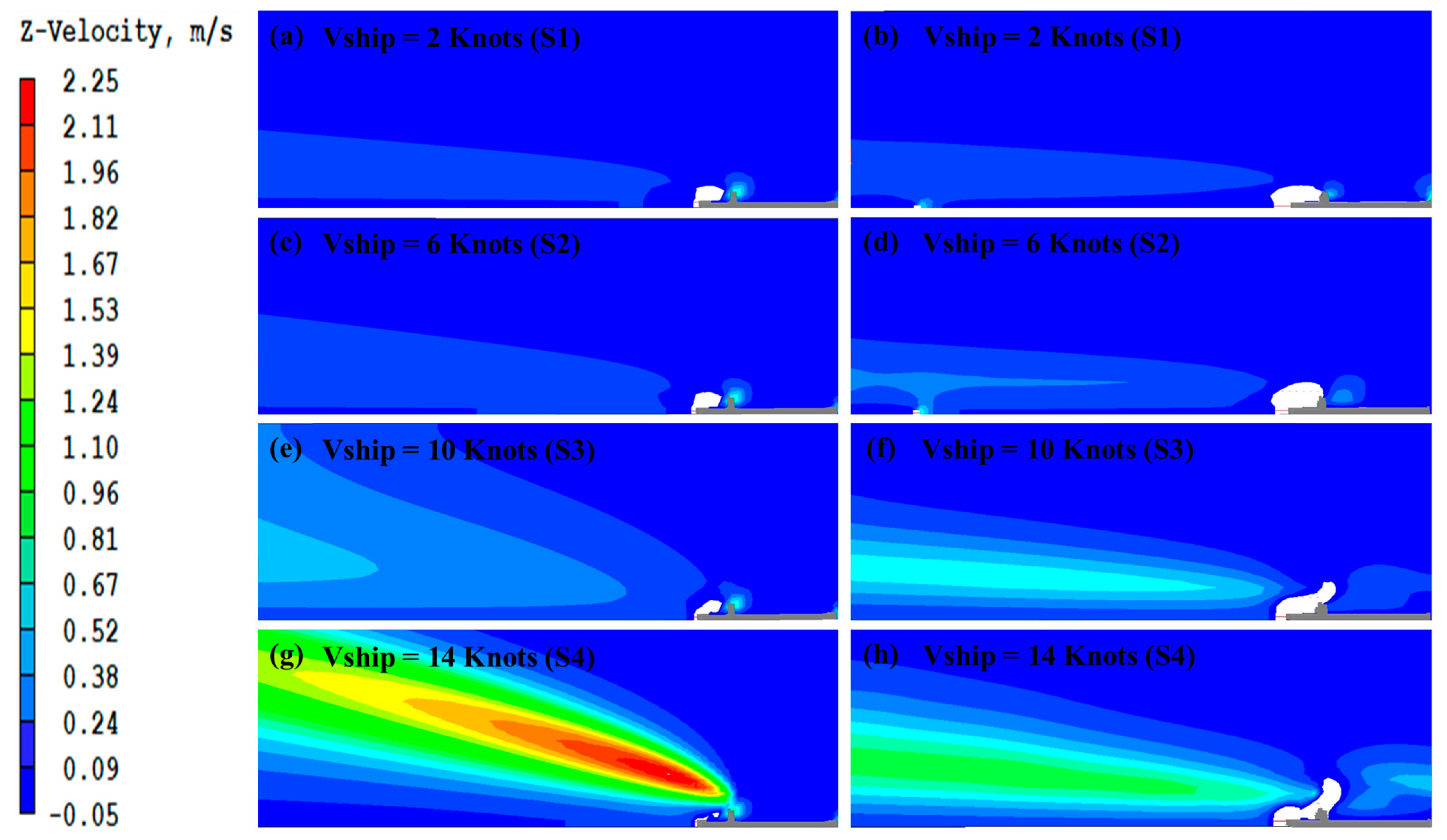
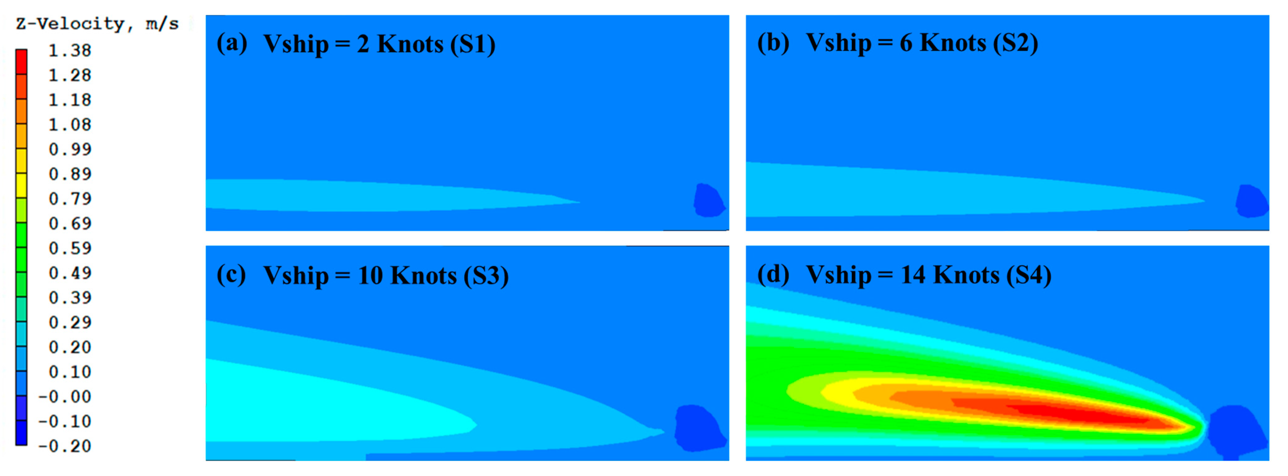
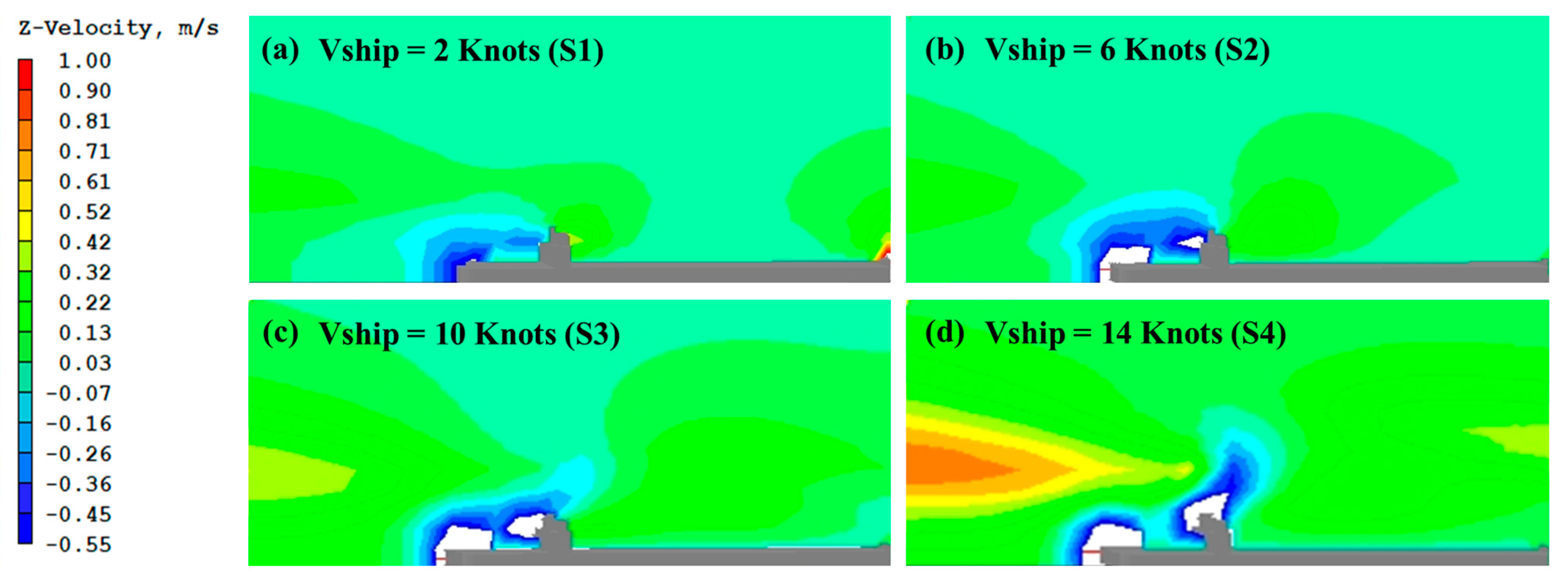
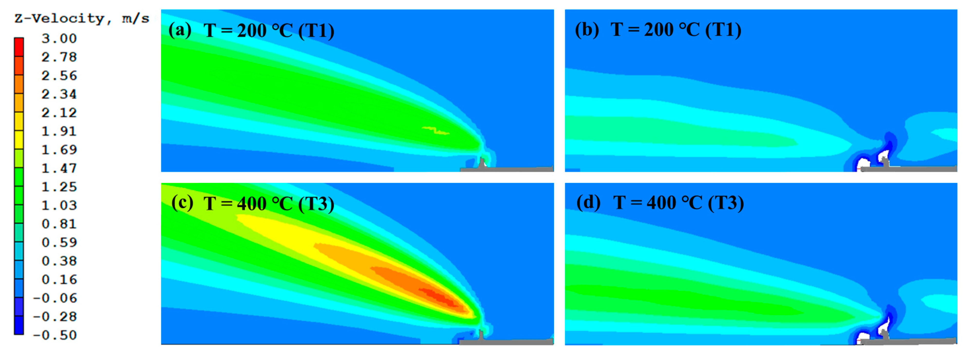
3.3. The Flow Field Characteristics That Cause Differences in the Smoke Plume Rising Height

The dH+ is strongly affected by wind speed and ship speed, especially at low wind speeds and high ship speeds. In these cases, the rising height of the smoke from the moving source simulation scheme is significantly smaller than from the stationary source simulation scheme. This difference between the two is, however, small at high wind speeds. Wind speed is an important parameter affecting smoke plume rising [40,49,50], with smoke plumes rising higher due to buoyancy in the low wind scenario. When the wind speed is high, the dynamic and buoyancy mechanisms for smoke rising become weak, causing small smoke rising heights. This effect is applicable to both stationary and moving sources, only the degree of the effect may vary. Section 3.1, for example, shows that the H+ is small for both the simulation schemes at high wind speeds and therefore the corresponding dH+ at high wind speeds is also small. This is also reflected in the flow field characteristics obtained from the numerical simulations. Figure 8c,d shows that the vertical velocity fields for the stationary and moving sources are very similar for wind speeds of 12 m/s. With a decrease in the wind speed, the dynamic and buoyant effects of the rising smoke increase. The lower the wind speed, the more the smoke rises. The dynamic and buoyant effects of the rising smoke from the moving ship compared to the stationary ship are reduced due to the high dispersion of flue gas. The lack of experimental studies on these aspects makes it necessary to use numerical simulations to illustrate the rising smoke plume. The vertical velocity behind the ship has a high value in the plume’s path, indicating that the plume has a tendency to rise in this area. The vertical velocity of the stationary source results in a wind speed of 3 m/s (Figure 8a), which is much larger than a wind speed of 12 m/s (Figure 8c), due to enhanced kinetic and thermal rising. The vertical velocity of the moving source at this wind speed (Figure 8b) is much smaller than that of the stationary source due to the dispersion of the momentum, the heat release along the course of the movement, and the weakened contribution to plume rising.
The higher the ship speed, the greater the difference between the rising height of the plume for both the moving source scheme and the stationary source. These simulation results are in line with the results of the theoretical analysis, since the ship movement itself is the key factor causing the difference between the plume rising height of the two schemes, and since both the dynamic and thermal mechanisms of the rising smoke are weakened when the ship moves. The specific reasons for this characteristic of dH+ can be analyzed together with the numerical simulation results of the flow field. Figure 9 shows that the vertical velocity and the extent of the region behind the moving ship where the smoke rises are much smaller than those behind the stationary ship at higher speeds (S3 and S4). The average height of the high-value area of the vertical velocity of the stationary source is also higher than that of the moving source, which leads to a larger dH+ being statistically obtained at higher ship speeds as well. The difference between the two simulations is also the same for the lower ship speeds (S1 and S2). In this case, the difference is, however, much less significant than for the higher ship speeds. The higher the ship speed is, the greater the difference between the flow field behind the moving ship and the stationary ship, which causes a correspondingly greater dH+.
Ship movement includes both exhaust outlet movement and hull movement that all influence the differences in results between the moving source scheme and the stationary source scheme. Numerical experiments were carried out to simulate these two factors separately to further understand the actual effect of these two factors on the dH+. Figure 10 shows the numerical simulation result of only the exhaust outlet movement. The patterns and values of the vertical velocity fields are relatively similar for both sets when comparing them with the simulation results for the moving source in Figure 9. This indicates that of the two movement-related factors, the central factor affecting the flue gas rising for the moving source scheme and the dH+ for both schemes is the movement of the exhaust outlet. Moving the exhaust outlet has a greater effect than moving the hull. Even though the exit velocity is greater at higher ship speeds, the initial momentum and dispersive release of the initial heat due to exhaust outlet movement have a greater overall effect. The effect of the hull movement is however also noteworthy. The results in Section 3.1 show that the smoke rising height of a moving ship first decreases and then increases with an increase in ship speed (Figure 4b). Figure 9 and Figure 10 show that the vertical velocity of S1 is overall slightly higher than that of S2. The vertical velocity field near the hull, however, (Figure 11), shows a negative region near the hull due to the movement of the ship, which increases with increasing ship speed. The smoke plume rising height decreases in this negative area. Even though the downwash of smoke near the hull is stronger at high ship speeds than at low ship speeds for the ship speeds S2 to S4, high ship speeds have a stronger rising effect in the area behind the ship. The smoke rising height, therefore, increases significantly due to the increase in ship speed (Figure 4b). The plume rising height of the S1 to S2 section in Figure 4b decreases, which may be due to the greater downwash caused by the hull at S2 than at S1 (Figure 11).
The effect of the dispersed release of the flue gas momentum and the heat in the moving source ship simulation scenario was mentioned several times in the previous analysis and discussion. Figure 12 and Figure 13 show the relevant simulation results for the effects caused by heat dispersion. Figure 12 shows that the moving source heat release is dispersed, and that the moving source scheme achieves temperature equilibrium with the ambient air within a relatively small range after the hot flue gas is emitted compared to the stationary source scenario. The contribution of the thermal buoyancy effects to the vertical velocity is, therefore, smaller in value (Figure 13).

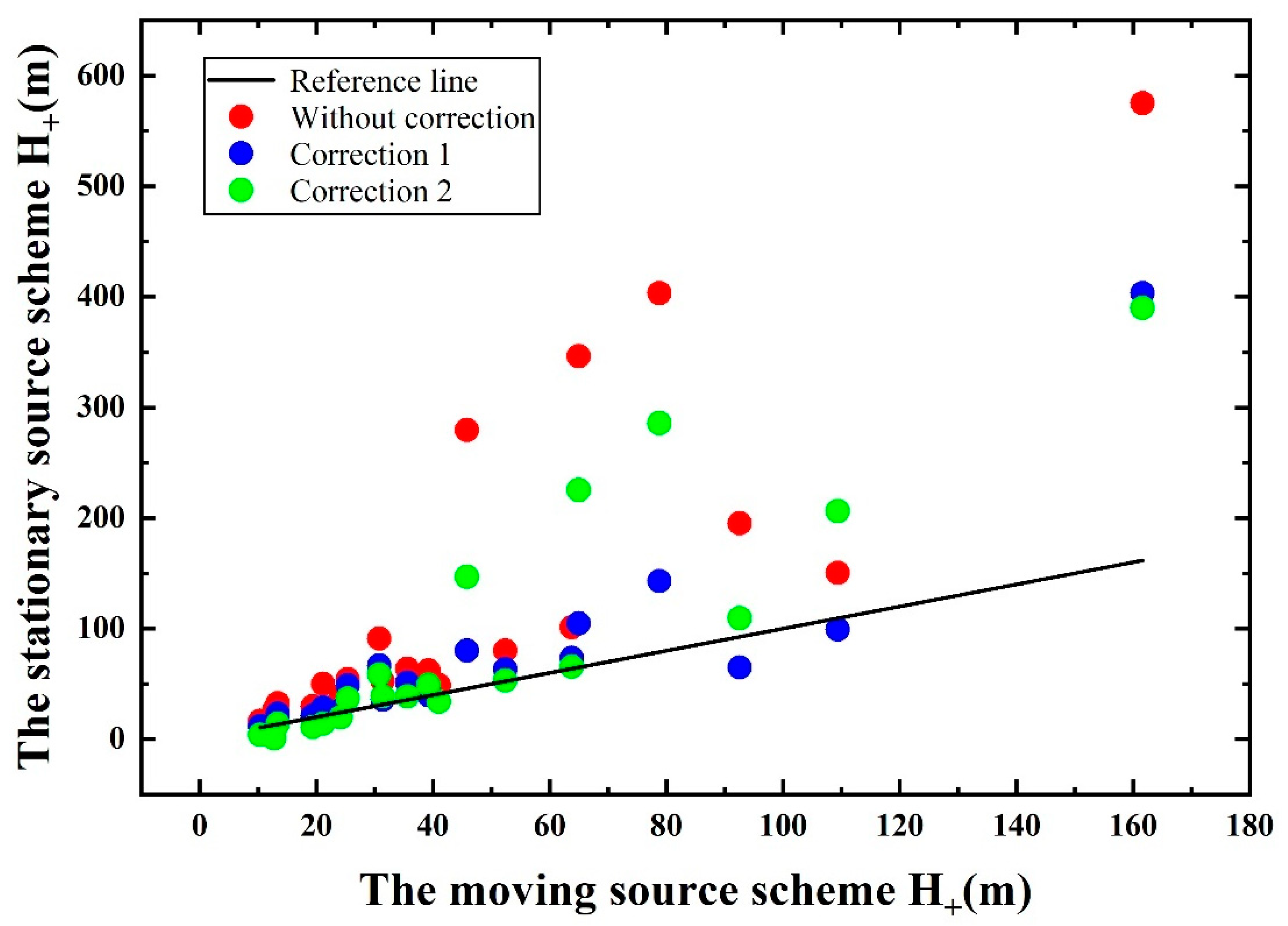
3.4. Simplified Calculation Methods for Simulating the Rising Smoke Plume of a Moving Ship with a Stationary Source Scheme

The effective height of the rising source plume is an important factor affecting the ambient concentration and distribution of pollutants. The uplift formula commonly used in the dispersion simulations is only applicable to stationary sources and not to moving sources [19,51]. The influence of the ship movement is therefore usually not considered in modeling studies of exhaust pollutants from moving sources on ships [20,52,53]. To obtain more accurate simulation results with limited computational cost, this study, therefore, attempts to establish a simplified method for approximating the rising plume from a moving ship using a stationary source simulation scheme.
When the ship is in motion, especially at high speeds, both the dynamic rising effect and the thermal rising effect are weaker due to the dispersed release of the momentum and heat from the flue gases. This results in lower plume rising for moving ships than for stationary sources. The kinetic and thermal effects of the flue gas emissions are directly related to the flue gas exit velocity and the flue gas exit temperature of the ships. To approximate the attenuating effect of the flue gas dynamic rising and the thermal rising, two correction schemes were considered. These included correcting the flue gas exit velocity or the flue gas exit temperature. The aim was to correct the smoke plume rising height of the stationary source simulation scheme at the flue gas exit velocity ( V e x i t ) or the flue gas exit temperature ( T ) equal to or close to the smoke plume rising height of the moving source simulation scheme at the actual flue gas exit velocity ( V e x i t ) or the actual flue gas exit temperature (T).
The dH+ results obtained in the above scenario of a higher ship speed and a lower wind speed (ship speed ≥ 10 knots and wind speed ≤ 6 m/s), were used in a stepwise regression fitting with wind speed ( V w i n d ), ship speed ( V s h i p ), flue gas exit velocity ( V e x i t ), and flue gas exit temperature (T) as independent variables. This yielded the following correction equations for V e x i t (Equation (1)) or T (Equation (2)):
V e x i t = 0.491913 V e x i t 0.05309 V w i n d 0.00679 V s h i p 0.000025 T + 0.881252
T = 0.687404 T 10.795358 V w i n d 0.191119 V e x i t + 0.438427 V s h i p 33.10996
where V e x i t is the corrected flue gas exit velocity in m/s; V e x i t is the actual flue gas exit velocity in m/s; V w i n d is the wind speed in m/s; V s h i p is the ship speed in knots; T is the actual flue gas exit temperature in °C; and T is the corrected flue gas exit temperature in °C.
For the last step of the stepwise regression fitting, the R2 for Equation (1) is 0.77 and the R2 for Equation (2) is 0.99. The effects of the two corrected methods were compared. To do this, the corrected parameter values were used to simulate the stationary source scheme for 20 CFD model cases in this study for the low wind speed and high ship speed scenarios. Then the modified stationary source scheme was compared with the moving source scheme for the plume’s rising heights. Table 4 shows the case parameters, together with the corrected flue gas exit velocity and flue gas exit temperature. The tested cases cover different combinations of flue gas exit velocity and flue gas temperature for high ship speed and low wind speed conditions. Figure 14 shows the approximate simulated plume rising heights at 1 km downwind for the stationary source scheme compared to the moving source scheme. These cases were introduced in Section 2, therefore, the stationary source scheme results shown in Section 3.1 are also compared in Figure 14 (i.e., the group without correction).
The relative error ( R d H + ) between the moving source simulation and the stationary source simulation was calculated to quantitatively assess the effect of the correction methods. This was done by taking H+ at 100 m intervals within 1 km behind the chimney for each simulation scheme, and was calculated as follows:
R d H + = ( S i M i M i ) × 100 %
where S i and M i are the stationary source ship plume rising height and the moving source ship plume rising height.
Table 4 presents the statistical results, where R ¯ d H + is the mean of 10 R d H + values calculated for each simulation scheme using Equation (3). An R ¯ d H + greater than 0 means that the H + of the stationary source simulation scheme is generally higher than the moving source simulation scheme, while the opposite is lower than the H + of the moving source simulation scheme. The closer the absolute value of R ¯ d H + is to zero, the closer the H + of the stationary source simulation is to that of the moving source simulation. For 20 validation cases, the average of R ¯ d H + for the three stationary source simulations (without correction, corrected V e x i t , and corrected T ) were 135.38%, 5.48%, and 60.07%, respectively. The average of R ¯ d H + with both the corrected V e x i t and the T were lower than the R ¯ d H + without correction, while the average of R ¯ d H + with the corrected V e x i t was lower than that with the corrected T . For the results of the two correction schemes, the results with the V e x i t correction are slightly better than those with the T correction.
The simulation time of the simulation experiment was found to be greatly reduced by using the stationary source scheme to approximate the calculation of the smoke plume rising height of the moving source ship. The simulation results of the validation cases reveal that the approximate simulation results are similar to those from the moving source scheme. These simulation results are expected to be used to improve the problem of the underestimation of atmospheric pollutants in the mesoscale model simulations of ships, specifically the V e x i t correction scheme (shown in Equation (1)).
By using this correction scheme, the simultaneous correction of the flue gas exit velocity and the flue gas exit temperature is also feasible. Since both these parameters affect the rising height of the smoke plume, there would be an infinite number of parameter combination options for a simultaneous correction. The simultaneous correction was therefore not considered in this study.

4. Conclusions

To understand the smoke plume rising characteristics of a moving ship, this study simulated the smoke plume characteristics of the moving ship by using parameterized values in the CFD software PHOENICS 6.0. The rising smoke plume characteristics were simulated and analyzed for the stationary source scheme and the moving source scheme. The relative variation in the simulation results of the moving source scheme was analyzed using the simulation results of the stationary source scheme. Finally, simplified calculation methods were established to approximate the rising smoke plume of the moving ship using the stationary source scheme parameters.
The main parameters affecting the rising smoke plume of the moving ships include the ship speed, the environmental wind speed, the flue gas exit velocity, and the flue gas exit temperature. For the two simulation schemes (stationary source and moving source), the plume rising height decreased with an increase in wind speed and increased with an increase in the flue gas exit velocity and the flue gas exit temperature. The difference between the two is reflected in the results of the different ship speeds. In the stationary source scheme, the plume’s rising height increases with an increase in ship speed. In the moving source scheme, the plume’s rising height first decreases and then increases with an increase in ship speed. The lowest value appears when the ship speed is 6 knots. The wind speed and the ship speed mainly influence the plume rising height difference between the stationary source and the moving source simulation schemes.
This study used simplified calculation methods to approximate the plume rising height of a moving ship using a stationary source simulation scheme. Stepwise regression fitting was used to determine the corrected flue gas exit velocity ( V e x i t ) and the corrected flue gas exit temperature ( T ). For the validation cases, the average relative error of the stationary source simulation scheme without correction, the stationary source scheme with corrected V e x i t , and the stationary source scheme with corrected T versus the moving source scheme were 135.38%, 5.48%, and 60.07%, respectively. These two correction methods can potentially improve the modeled underestimation of air pollutant emissions from moving ships in the mesoscale model, with the corrected V e x i t method being more effective.
Future work plans to carry out field experimentation in more different ports based on the results of this exploratory study on the plume rising height of moving ships, and use more ship cases to validate the plume rising height correction formulas proposed in this study. We plan to compare the simulation results with the field experimentation results to further study the mechanism of the plume rising of moving ships, hoping to provide some reference for the study of plume dispersion of moving ships at port.

Author Contributions

Software, writing—original draft, writing—review and editing, visualization, J.L.; data curation, investigation, J.S.; resources, data curation, Y.X.; supervision, conceptualization, methodology, project administration, Q.Y.; methodology, project administration, Y.Z.; supervision, project administration, W.M. All authors have read and agreed to the published version of the manuscript.

Funding

This research was funded by the Key-Area Research and Development Program of Guangdong Province, grant number 2020B1111360001, the National Natural Science Foundation of China, grant number 42077195, and the research project funded by the Ministry of Industry and Information Technology of China, grant number MC-202019-C08. And the APC was funded by the Key-Area Research and Development Program of Guangdong Province, grant number 2020B1111360001.

Acknowledgments

This study was supported by the Research Project of Environmental Protection in Zhejiang Province (2019A003).

Conflicts of Interest

The authors declare no conflict of interest.

Appendix A

Table A1. Basic information of the port of the ship sample in Dapeng Bay, Shenzhen in June 2018.
Main Engine Stack Information
NumberSample of ShipDiameter (m)ME Power (kW)Exhaust Gas Temperature (℃)Speed Far away 1 km from Port (Knots)
1MSC DEILA2.5572,240/5.6
2AXEL MAERSK253,60020012.8
3MATHILDE MAERSK3.558,6003506.6
4CZECH1.3838,59020012
5HYUNDAI HONGKONG0.893,1206015.4
6MAERSK EINDHOVEN2.86668,6404006
7MSC BERYL3.345,7162506.3
8SEAMAX BRIDGEPORT2.169,467.532012.8
9MOL TRADITION159,2502753.3
10MSC BETTINA1.845,5003055.3
11NORTHERN JUVENILE2.257,10015712.8
12MAERSK SARNIA6.45561,9003238.2
13MOL CONTINUITY2.356,18525011.5
14MALIK AL ASHTAR2.871,7703505.5
15MSC LAURENCE161,36530011.3
16MSC SONIA373,316.882204.4
17APL LION CITY2.76662,0303007.6
18APL PARIS3.31854,12022011
19CMA CGM COLUMBA3.16572,2403275.6
20HYUNDAI DREAM2.41648,5102802.2
21KOTA PANJANG2.2642,3502008.7
22MONACO MAERSK1.72262,0003400.8
23MSC MIRJAM2.660,8503235
24MSC PALOMA3.1245,511/4
25MSC ROMA2.868,52030010.9
26NYK WREN10.4528,3101703.8
27OSAKA EXPRESS2.84634,50018814.5
28OOCL SEOUL2.668,443.233010.7
29TOLEDO TRIUMPH2.348,9003005.2
Table A2. Flus gas exit velocity corresponding to ship speed of the port of the ship sample in Dapeng Bay, Shenzhen in June 2018.
Exhaust Gas Exit Velocity Corresponding to Ship Speed (m/s)
NumberSample of ShipShip Speed at 2 KnotsShip Speed at 6 KnotsShip Speed at 10 KnotsShip Speed at 14 Knots
1MSC DEILA0.091.385.6614.07
2AXEL MAERSK0.071.496.7417.04
3MATHILDE MAERSK0.300.632.736.80
4CZECH1.262.3510.3726.15
5HYUNDAI HONGKONG9.0614.0555.70146.23
6MAERSK EINDHOVEN0.520.642.846.80
7MSC BERYL0.260.461.945.01
8SEAMAX BRIDGEPORT///15.46
9MOL TRADITION0.307.3431.3878.86
10MSC BETTINA0.061.286.1015.94
11NORTHERN JUVENILE0.731.035.0712.82
12MAERSK SARNIA0.090.090.882.23
13MOL CONTINUITY0.660.662.928.00
14MALIK AL ASHTAR0.030.773.538.89
15MSC LAURENCE/5.3423.4960.43
16MSC SONIA0.030.883.799.80
17APL LION CITY/0.502.657.01
18APL PARIS/0.542.446.08
19CMA CGM COLUMBA/0.943.9410.03
20HYUNDAI DREAM/0.964.0310.27
21KOTA PANJANG0.051.034.0410.25
22MONACO MAERSK/2.599.8524.38
23MSC MIRJAM/1.044.3111.25
24MSC PALOMA/0.753.268.05
25MSC ROMA/0.994.3411.089
26NYK WREN/0.040.19/
27OSAKA EXPRESS0.270.723.127.33
28OOCL SEOUL/0.913.9310.18
29TOLEDO TRIUMPH/0.622.576.84

References

  1. Zhang, Y.; Yang, X.; Brown, R.; Yang, L.P.; Morawska, L.; Ristovski, Z.; Fu, Q.Y.; Huang, C. Shipping emissions and their impacts on air quality in China. Sci. Total Environ. 2017, 581, 186–198. [Google Scholar] [CrossRef] [PubMed]
  2. Merico, E.; Cesari, D.; Gregoris, E.; Gambaro, A.; Cordella, M.; Contini, D. Shipping and Air Quality in Italian Port Cities: State-of-the-Art Analysis of Available Results of Estimated Impacts. Atmosphere 2021, 12, 536. [Google Scholar] [CrossRef]
  3. Viana, M.; Hammingh, P.; Colette, A.; Querol, X.; Degraeuwe, B.; de Vlieger, I.; van Aardenne, J. Impact of maritime transport emissions on coastal air quality in Europe. Atmos. Environ. 2014, 90, 96–105. [Google Scholar] [CrossRef]
  4. Fan, Q.Z.; Zhang, Y.; Ma, W.C.; Ma, H.X.; Feng, J.L.; Yu, Q.; Yang, X.; Ng, S.K.W.; Fu, Q.Y.; Chen, L.M. Spatial and Seasonal Dynamics of Ship Emissions over the Yangtze River Delta and East China Sea and Their Potential Environmental Influence. Environ. Sci. Technol. 2016, 50, 1322–1329. [Google Scholar] [CrossRef]
  5. Zhang, C.; Shi, Z.B.; Zhao, J.R.; Zhang, Y.; Yu, Y.; Mu, Y.C.; Yao, X.H.; Feng, L.M.; Zhang, F.; Chen, Y.J.; et al. Impact of air emissions from shipping on marine phytoplankton growth. Sci. Total Environ. 2021, 769, 145488. [Google Scholar] [CrossRef] [PubMed]
  6. Li, Q.Y.; Badia, A.; Fernandez, R.P.; Mahajan, A.S.; Lopez-Norena, A.; Zhang, Y.; Wang, S.S.; Puliafito, E.; Cuevas, C.A.; Saiz-Lopez, A. Chemical Interactions Between Ship-Originated Air Pollutants and Ocean-Emitted Halogens. J. Geophys. Res.-Atmos. 2021, 126, e2020JD034175. [Google Scholar] [CrossRef]
  7. Wang, X.N.; Shen, Y.; Lin, Y.F.; Pan, J.; Zhang, Y.; Louie, P.K.K.; Li, M.; Fu, Q.Y. Atmospheric pollution from ships and its impact on local air quality at a port site in Shanghai. Atmos. Chem. Phys. 2019, 19, 6315–6330. [Google Scholar] [CrossRef]
  8. Blatcher, D.J.; Eames, I. Compliance of Royal Naval ships with nitrogen oxide emissions legislation. Mar. Pollut. Bull. 2013, 74, 10–18. [Google Scholar] [CrossRef]
  9. Zhao, J.R.; Zhang, Y.; Xu, H.R.; Tao, S.; Wang, R.; Yu, Q.; Chen, Y.; Zou, Z.; Ma, W.C. Trace Elements from Ocean-Going Vessels in East Asia: Vanadium and Nickel Emissions and Their Impacts on Air Quality. J. Geophys. Res.-Atmos. 2021, 126, e2020JD033984. [Google Scholar] [CrossRef]
  10. Zhao, M.J.; Zhang, Y.; Ma, W.C.; Fu, Q.Y.; Yang, X.; Li, C.L.; Zhou, B.; Yu, Q.; Chen, L.M. Characteristics and ship traffic source identification of air pollutants in China’s largest port. Atmos. Environ. 2013, 64, 277–286. [Google Scholar] [CrossRef]
  11. Zhang, F.; Chen, Y.J.; Cui, M.; Feng, Y.L.; Yang, X.; Chen, J.M.; Zhang, Y.; Gao, H.W.; Tian, C.G.; Matthias, V.; et al. Emission factors and environmental implication of organic pollutants in PM emitted from various vessels in China. Atmos. Environ. 2019, 200, 302–311. [Google Scholar] [CrossRef]
  12. Sun, J.F.; Chen, H.; Mao, J.B.; Zhao, J.R.; Zhang, Y.; Wang, L.; Wang, X.K.; Ouyang, H.L.; Tang, X.; George, C.; et al. Secondary Inorganic Ions Characteristics in PM2.5 Along Offshore and Coastal Areas of the Megacity Shanghai. J. Geophys. Res.-Atmos. 2021, 126, e2021JD035139. [Google Scholar] [CrossRef]
  13. Lloret, J.; Carreno, A.; Caric, H.; San, J.; Fleming, L.E. Environmental and human health impacts of cruise tourism: A review. Mar. Pollut. Bull. 2021, 173, 112979. [Google Scholar] [CrossRef] [PubMed]
  14. Liu, H.; Fu, M.L.; Jin, X.X.; Shang, Y.; Shindell, D.; Faluvegi, G.; Shindell, C.; He, K.B. Health and climate impacts of ocean-going vessels in East Asia. Nat. Clim. Chang. 2016, 6, 1037–1041. [Google Scholar] [CrossRef]
  15. Barregard, L.; Molnar, P.; Jonson, J.E.; Stockfelt, L. Impact on Population Health of Baltic Shipping Emissions. Int. J. Environ. Res. Public Health 2019, 16, 1954. [Google Scholar] [CrossRef]
  16. Jahangiri, S.; Nikolova, N.; Tenekedjiev, K. Health risk assessment of engine exhaust emissions within Australian ports: A case study of Port of Brisbane. Environ. Pract. 2019, 21, 20–35. [Google Scholar] [CrossRef]
  17. Mandal, A.; Biswas, J.; Farooqui, Z.; Roychowdhury, S. A detailed perspective of marine emissions and their environmental impact in a representative Indian port. Atmos. Pollut. Res. 2021, 12, 101194. [Google Scholar] [CrossRef]
  18. Lateb, M.; Meroney, R.N.; Yataghene, M.; Fellouah, H.; Saleh, F.; Boufadel, M.C. On the use of numerical modelling for near-field pollutant dispersion in urban environments-A review. Environ. Pollut. 2016, 208, 271–283. [Google Scholar] [CrossRef]
  19. Marelle, L.; Thomas, J.L.; Raut, J.C.; Law, K.S.; Jalkanen, J.P.; Johansson, L.; Roiger, A.; Schlager, H.; Kim, J.; Reiter, A.; et al. Air quality and radiative impacts of Arctic shipping emissions in the summertime in northern Norway: From the local to the regional scale. Atmos. Chem. Phys. 2016, 16, 2359–2379. [Google Scholar] [CrossRef]
  20. Wang, R.N.; Tie, X.X.; Li, G.H.; Zhao, S.Y.; Long, X.; Johansson, L.; An, Z.S. Effect of ship emissions on O-3 in the Yangtze River Delta region of China: Analysis of WRF-Chem modeling. Sci. Total Environ. 2019, 683, 360–370. [Google Scholar] [CrossRef]
  21. Feng, J.L.; Zhang, Y.; Li, S.S.; Mao, J.B.; Patton, A.P.; Zhou, Y.Y.; Ma, W.C.; Liu, C.; Kan, H.D.; Huang, C.; et al. The influence of spatiality on shipping emissions, air quality and potential human exposure in the Yangtze River Delta/Shanghai, China. Atmos. Chem. Phys. 2019, 19, 6167–6183. [Google Scholar] [CrossRef]
  22. Murena, F.; Mocerino, L.; Quaranta, F.; Toscano, D. Impact on air quality of cruise ship emissions in Naples, Italy. Atmos. Environ. 2018, 187, 70–83. [Google Scholar] [CrossRef]
  23. Iris, C.; Lam, J.S.L. A review of energy efficiency in ports: Operational strategies, technologies and energy management systems. Renew. Sustain. Energy Rev. 2019, 112, 170–182. [Google Scholar] [CrossRef]
  24. Lonati, G.; Cernuschi, S.; Sidi, S. Air quality impact assessment of at-berth ship emissions. Case-study for the project of a new freight port. Sci. Total Environ. 2010, 409, 192–200. [Google Scholar] [CrossRef]
  25. Holmes, N.S.; Morawska, L. A review of dispersion modelling and its application to the dispersion of particles: An overview of different dispersion models available. Atmos. Environ. 2006, 40, 5902–5928. [Google Scholar] [CrossRef]
  26. Poplawski, K.; Setton, E.; McEwen, B.; Hrebenyk, D.; Graham, M.; Keller, P. Impact of cruise ship emissions in Victoria, BC, Canada. Atmos. Environ. 2011, 45, 824–833. [Google Scholar] [CrossRef]
  27. Toscano, D.; Marro, M.; Mele, B.; Murena, F.; Salizzoni, P. Assessment of the impact of gaseous ship emissions in ports using physical and numerical models: The case of Naples. Build. Environ. 2021, 196, 107812. [Google Scholar] [CrossRef]
  28. Xu, Y.N.; Yu, Q.; Zhang, Y.; Ma, W.C. Numerical Study on the Plume Behavior of Multiple Stacks of Container Ships. Atmosphere 2021, 12, 600. [Google Scholar] [CrossRef]
  29. Pasquill, F.; Michael, P. Atmospheric Diffusion, 2nd edition. Phys. Today 1977, 30, 55–57. [Google Scholar] [CrossRef]
  30. Seshadri, V.; Singh, S.; Kulkarni, P. Study of Problem of Exhaust Smoke Ingress into GT Intakes of a Naval Ship. J. Ship Technol. 2006, 2. [Google Scholar]
  31. Huang, J.T.; Carrica, P.M.; Stern, F. A method to compute ship exhaust plumes with waves and wind. Int. J. Numer. Methods Fluids 2012, 68, 160–180. [Google Scholar] [CrossRef]
  32. Tominaga, Y.; Stathopoulos, T. CFD simulation of near-field pollutant dispersion in the urban environment: A review of current modeling techniques. Atmos. Environ. 2013, 79, 716–730. [Google Scholar] [CrossRef]
  33. Kulkarni, P.R.; Singh, S.N.; Seshadri, V. Comparison of CFD simulation of Exhaust Smoke-Superstructure Interaction on a Ship with Experimental Data. In Proceedings of the 10th Naval Platform Technology Seminar NPTS-05, Singapore, 17 May 2005. [Google Scholar]
  34. Duy, T.N.; Hino, T.; Suzuki, K. Numerical study on stern flow fields of ship hulls with different transom configurations. Ocean. Eng. 2017, 129, 401–414. [Google Scholar] [CrossRef]
  35. Watson, N.A.; Kelly, M.F.; Owen, I.; Hodge, S.J.; White, M.D. Computational and experimental modelling study of the unsteady airflow over the aircraft carrier HMS Queen Elizabeth. Ocean. Eng. 2019, 172, 562–574. [Google Scholar] [CrossRef]
  36. Kumar, P.; Singh, S.K.; Ngae, P.; Feiz, A.A.; Turbelin, G. Assessment of a CFD model for short-range plume dispersion: Applications to the Fusion Field Trial 2007 (FFT-07) diffusion experiment. Atmos. Res. 2017, 197, 84–93. [Google Scholar] [CrossRef]
  37. Mao, J.B.; Zhang, Y.; Yu, F.Q.; Chen, J.M.; Sun, J.F.; Wang, S.S.; Zou, Z.; Zhou, J.; Yu, Q.; Ma, W.C.; et al. Simulating the impacts of ship emissions on coastal air quality: Importance of a high-resolution emission inventory relative to cruise-and land-based observations. Sci. Total Environ. 2020, 728, 138454. [Google Scholar] [CrossRef]
  38. Vijayakumar, R.; Singh, S.N.; Seshadri, V. CFD prediction of the trajectory of hot exhaust from the funnel of a naval ship in the presence of ship superstructure. Int. J. Marit. Eng. 2014, 156, 1–23. [Google Scholar] [CrossRef]
  39. Bayraktar, S.; Safa, A.; Yilmaz, T. Cfd and analytical analysis of exhaust system of a gas turbine used in a ship. In Proceedings of the International Conference on Numerical Analysis and Applied Mathematics, Corfu, Greece, 16–20 September 2007. [Google Scholar]
  40. Fujimura, A.; Matt, S.; Soloviev, A.; Maingot, C.; Rhee, S.H. The impact of thermal stratification and wind stress on sea surface features in sar imagery. In Proceedings of the IEEE International Geoscience and Remote Sensing Symposium (IGARSS), Vancouver, BC, Canada, 24–29 July 2011. [Google Scholar]
  41. Kumaresh, S.; Kim, M.Y.; Kim, C. Numerical investigation of plume dispersion characteristics for various ambient flow velocities. J. Mech. Sci. Technol. 2019, 33, 4511–4519. [Google Scholar] [CrossRef]
  42. Marro, M.; Salizzoni, P.; Cierco, F.X.; Korsakissok, I.; Danzi, E.; Soulhac, L. Plume rise and spread in buoyant releases from elevated sources in the lower atmosphere. Environ. Fluid Mech. 2014, 14, 201–219. [Google Scholar] [CrossRef]
  43. Edalati-nejad, A.; Ghodrat, M.; Fanaee, S.A.; Simeoni, A. Numerical Simulation of the Effect of Fire Intensity on Wind Driven Surface Fire and Its Impact on an Idealized Building. Fire-Switz. 2022, 5, 17. [Google Scholar] [CrossRef]
  44. Edalati-nejad, A.; Fanaee, S.A.; Ghodrat, M.; Salehi, F.; Khadem, J. The time dependent investigation of methane-air counterflow diffusion flames with detailed kinetic and pollutant effects into a micro/macro open channel. Case Stud. Therm. Eng. 2020, 18, 100603. [Google Scholar] [CrossRef]
  45. Kulkarni, P.R.; Singh, S.N.; Seshadri, V. Parametric studies of exhaust smoke-superstructure interaction on a naval ship using CFD. Comput. Fluids 2007, 36, 794–816. [Google Scholar] [CrossRef]
  46. Liu, C.; Li, Q.L.; Zhao, W.; Wang, Y.Q.; Ali, R.; Huang, D.; Lu, X.X.; Zheng, H.; Wei, X.L. Spatiotemporal Characteristics of Near-Surface Wind in Shenzhen. Sustainability 2020, 12, 739. [Google Scholar] [CrossRef]
  47. Liu, Z.M.; Lu, X.H.; Feng, J.L.; Fan, Q.Z.; Zhang, Y.; Yang, X. Influence of Ship Emissions on Urban Air Quality: A Comprehensive Study Using Highly Time-Resolved Online Measurements and Numerical Simulation in Shanghai. Environ. Sci. Technol. 2017, 51, 202–211. [Google Scholar] [CrossRef] [PubMed]
  48. Bai, S.B.; Wen, Y.Q.; He, L.; Liu, Y.M.; Zhang, Y.; Yu, Q.; Ma, W.C. Single-Vessel Plume Dispersion Simulation: Method and a Case Study Using CALPUFF in the Yantian Port Area, Shenzhen (China). Int. J. Environ. Res. Public Health 2020, 17, 7831. [Google Scholar] [CrossRef]
  49. Tohidi, A.; Kaye, N.B. Highly buoyant bent-over plumes in a boundary layer. Atmos. Environ. 2016, 131, 97–114. [Google Scholar] [CrossRef]
  50. Velamati, R.K.; Vivek, M.; Goutham, K.; Sreekanth, G.R.; Dharmarajan, S.; Goel, M. Numerical study of a buoyant plume from a multi-flue stack into a variable temperature gradient atmosphere. Environ. Sci. Pollut. Res. 2015, 22, 16814–16829. [Google Scholar] [CrossRef]
  51. Villasenor, R.; Magdaleno, M.; Quintanar, A.; Gallardo, J.C.; Lopez, M.T.; Jurado, R.; Miranda, A.; Aguilar, M.; Melgarejo, L.A.; Palmerin, E.; et al. An air quality emission inventory of offshore operations for the exploration and production of petroleum by the Mexican oil industry. Atmos. Environ. 2003, 37, 3713–3729. [Google Scholar]
  52. Molders, N.; Porter, S.E.; Cahill, C.F.; Grell, G.A. Influence of ship emissions on air quality and input of contaminants in southern Alaska National Parks and Wilderness Areas during the 2006 tourist season. Atmos. Environ. 2010, 44, 1400–1413. [Google Scholar]
  53. Yim, S.H.L.; Fung, J.C.H.; Lau, A.K.H. Use of high-resolution MM5/CALMET/CALPUFF system SO2 apportionment to air quality in Hong Kong. Atmos. Environ. 2010, 44, 4850–4858. [Google Scholar]
Figure 1. The ship model, the domain, and the grids in the CFD model: (a) model setting on the X–Z plane; (b) model setting on the Y–Z plane.
Atmosphere 13 01507 g001
Figure 2. The rising height (H+) of the smoke plume of the T2 group: (a) stationary source and (b) moving source.
Atmosphere 13 01507 g002
Figure 3. The rising height (H+) of the smoke plume of the V2 group: (a) stationary source and (b) moving source.
Atmosphere 13 01507 g003
Figure 4. The relative rate of change (RH+) in the H+ for the simulation schemes with influencing parameters: (a) stationary source and (b) the moving source (red dots indicate reference scenario: S2−V2−T2 scenario at a wind speed of 3 m/s).
Atmosphere 13 01507 g004
Figure 5. The rising height difference dH+ between the moving source scheme and the stationary source scheme at different wind speeds in the V2−T2 scenario.
Atmosphere 13 01507 g005
Figure 6. The rising height difference (dH+) between the moving source scheme and the stationary source scheme at different emission levels in the T2 scenario with a wind speed of 3 m/s.
Atmosphere 13 01507 g006
Figure 7. The rising height difference (dH+) between the moving source scheme and the stationary source scheme at different emission temperatures in the V2 scenario with a wind speed of 3 m/s.
Atmosphere 13 01507 g007
Figure 8. The vertical velocity contours in the S4−V2−T2 scenario: (a) stationary source when the wind speed is 3 m/s; (b) moving source when the wind speed is 3 m/s; (c) stationary source when the wind speed is 12 m/s; and (d) moving source when the wind speed is 12 m/s.
Atmosphere 13 01507 g008
Figure 9. The vertical velocity contours in the V2−T2 scenario with a wind speed of 3 m/s: (a,c,e,g) are the stationary sources and (b,d,f,h) are the moving sources.
Atmosphere 13 01507 g009
Figure 10. The vertical velocity contours influenced only by exhaust outlet movement in the V2−T2 scenario at wind speeds of 3 m/s: (ad) are S1, S2, S3, and S4 scenarios, respectively.
Atmosphere 13 01507 g010
Figure 11. The vertical velocity contours near the hull in the V2−T2 scenario with wind speeds of 3 m/s: (ad) are S1, S2, S3, and S4 scenarios, respectively.
Atmosphere 13 01507 g011
Figure 12. The vertical temperature contours in the S4-V2 scenario with a wind speed of 3 m/s: (a) stationary source of T1; (b) moving source of T1; (c) stationary source of T3; and (d) moving source of T3.
Atmosphere 13 01507 g012
Figure 13. The vertical velocity contours in the S4−V2 scenario with a wind speed of 3 m/s: (a) stationary source of T1; (b) moving source of T1; (c) stationary source of T3; and (d) moving source of T3.
Atmosphere 13 01507 g013
Figure 14. The comparison between the smoke plume rising height (H+) at 1 km downwind simulated by the three stationary source schemes (without correction; correction 1 that corrected V e x i t ; correction 2 that corrected T ) and the results of the moving source scheme in the validation cases (the dashed line is the 1:1 line as a reference).
Atmosphere 13 01507 g014
Table 1. Representative values of wind speed and ship speed.
ParameterValue RangeRepresentative Value
Ship speed (Knots)0–42 (S1 *)
4–86 (S2 *)
8–1210 (S3 *)
12–1614 (S4 *)
Wind speed (m/s)1.5–4.53
4.5–7.56
7.5–10.59
10.5–13.512
* Ship speed code.
Table 2. Flue gas exit velocity for the different emission scenarios.
Emission ScenariosFlue Gas Exit Velocity (m/s)
Ship Speed (Knots)SO2 Mass Fraction of Exhaust Gas Exit (C1)Emission LevelNumber
22.67 × 10⁻³LowS1-V10.26
MediumS1-V20.66
HighS1-V31.26
61.79 × 10⁻³LowS2-V10.46
MediumS2-V21.04
HighS2-V32.35
106.48 × 10⁻⁴LowS3-V12.01
MediumS3-V24.31
HighS3-V310.37
145.01 × 10⁻⁴LowS4-V15.01
MediumS4-V211.25
HighS4-V326.15
Table 3. Calculation domains and the number of grids for different ship speeds.
Ship Speed (Knots)Calculation Domain (m)Number of Grids
01800 × 150 × 900120 × 15 × 60
21800 × 150 × 450120 × 15 × 30
61800 × 150 × 450120 × 15 × 30
102400 × 150 × 450160 × 15 × 30
143000 × 150 × 450200 × 15 × 30
Table 4. The parameter settings and statistical differences of the verification cases in the CFD model.
Validation Case V s h i p   ( Knots ) V w i n d   ( m / s ) V e x i t   ( m / s ) T (℃) V e x i t
(m/s)
T
(°C)
R ¯ d H +   ( % )
Without Correction Correction   1   ( V e x i t ) Correction   2   ( T )
Case11034.312002.7770.5518.495.190.17
Case21034.313002.77139.29−12.61−21.54−21.84
Case31034.314002.77208.03−11.02−32.90−32.47
Case41032.013001.64139.7343.7736.0217.91
Case510310.373005.75138.13−10.10−53.25107.37
Case61064.312002.6138.1686.143.55−51.11
Case71064.313002.61106.9033.561.48−27.81
Case81064.314002.60175.6449.37−2.59−17.84
Case91062.013001.48107.3434.9611.23−30.51
Case1010610.373005.59105.745.59−22.40−14.24
Case1114311.252006.1670.97643.0812.73312.61
Case1214311.253006.15139.71561.45−11.51341.44
Case1314311.254006.15208.45535.64−10.43352.02
Case141435.013003.08140.9166.437.6241.75
Case1514326.1530013.48136.87284.94161.89164.09
Case1614611.252006.0038.5993.2416.27−14.57
Case1714611.253005.99107.3339.14−3.0418.48
Case1814611.254005.99176.0734.25−15.3914.69
Case191465.013002.92108.5285.6741.173.65
Case2014626.1530013.32104.48125.59−44.5537.64
Publisher’s Note: MDPI stays neutral with regard to jurisdictional claims in published maps and institutional affiliations.

