Article

Analysis of the Concentration of Emissions from the Spanish Fleet of Tugboats

by
Andrés Ortega-Piris
1,
Emma Diaz-Ruiz-Navamuel
1,*,
Alvaro Herrero Martinez
1,
Miguel A. Gutierrez
2 and
Alfonso-Isidro Lopez-Diaz
3
1
Ocean and Coastal Planning and Management R&D Group, School of Nautical Studies of Santander, University of Cantabria, C/Gamazo, 1, 39004 Santander, Spain
2
Department of Technology, Faculty of Science, Catholic University of Ávila, C/Canteros S/N, 05005 Ávila, Spain
3
Department of Electrical, Electronic, Automatic and Communications Engineering, School of Industrial and Aerospace Engineering, University of Castilla-La Mancha, Royal Arms Factory Avda, Calos III, SN, 45071 Toledo, Spain
*
Author to whom correspondence should be addressed.
Atmosphere 2022, 13(12), 2109; https://doi.org/10.3390/atmos13122109
Submission received: 11 November 2022 / Revised: 9 December 2022 / Accepted: 11 December 2022 / Published: 16 December 2022
(This article belongs to the Special Issue Impacts of Air Pollutants Emitted from Ships on Environment)

Abstract

:
At present, the sensitivity of society towards emissions in commercial maritime ports is increasing, which is reflected in the large number of studies on the control of emissions in them, perhaps because the most important commercial ports are located in cities with high population density. The objective of this work was to determine the greenhouse gas emissions caused by the activity of the Spanish tugboat fleet, studying the tugboat fleet of the eleven autonomous coastal Spanish communities from 2004 to 2017 and their impact on the carbon footprint of the country’s shipping sector. To do this, the methodology used by the International Maritime Organization for merchant ships to estimate the emissions of a tugboat fleet is formalized, and Gini concentration index methodology was applied to the concentration of emissions from this fleet. This has made it possible to obtain results on the distribution of the concentration of emissions from Spanish ports by region, age, and size, as well as to establish the profile of the tugboat port that pollutes the most and its carbon footprint. One of the results is that in the period analyzed, the concentration of emissions from the Spanish tugboat fleet increased if we looked at its distribution by region, and decreased if we look at its distribution by age and size. This is because tugboat activity was very different by region; however, their characteristics related to age and size evolved in a more homogeneous way.

1. Introduction

At present, the fight against climate change is one of the main challenges facing humanity. It is a generally accepted fact that human activity is the main cause of climate change. Since the industrial revolution, the concentration of greenhouse gases (GHGs) in the atmosphere has been increasing continuously, with adverse consequences for the planet.
In 1979, the First World Conference on Climate was held in Geneva, discussing global warming and its effects on human activity. The conference issued a statement urging the governments of the world to control and foresee potential changes in the climate caused by human beings that may be adverse for the well-being of humanity [1].
On 9 May 1992, the United Nations Framework Convention on Climate Change [2] was approved in New York. The objective of the convention was the stabilization of concentrations of greenhouse gases in the atmosphere. This level should be reached in sufficient time for ecosystems to adapt naturally to climate change, to ensure that food production is not threatened by it, and to allow economic development to continue in a sustainable manner. The convention would soon become the key central instrument of global efforts to combat global warming.
The first international recognition of the problem of climate change and the need to act was made in June 1992, within the framework of the Earth Summit held in Rio de Janeiro. Subsequently, the Kyoto Protocol of 1998 admitted that “The global atmospheric concentrations of carbon dioxide, methane and nitrous oxide have increased significantly since 1750 as a result of human activities, and now far exceed the pre-industrial values determined from ice samples that span back many thousands of years.” [3].
Finally, the so-called Paris agreement of 2015 concluded with the adoption of a historic agreement to combat climate change and promote measures and investments for a future that is low in carbon emissions, resilient, and sustainable. Its goal is to keep the temperature rise of this century below 2 °C.
Undoubtedly, global warming is a general problem and not only an environmental one, since it also affects the economy, trade, and security. In this sense, it demands a global response that integrates the different sectoral interests and the needs of all countries.
In this context, the global maritime transport sector has responded with sensitivity to the phenomenon of pollution, both that which may be caused by an accident and that which occurs during the daily operations of ships. In this regard, as a result of various events in the 1960s and 1970s, the maritime industry focused its efforts on the development of a regulatory framework that would limit pollution insofar as was possible. As a result of this work, the International Conference on Marine Pollution, convened by the International Maritime Organization (IMO) and held from 8 October to 2 November 1973, approved an international agreement to prevent pollution by ships, known as marine pollution (MARPOL). This new instrument came into force on 2 October 1983.
The convention contains rules aimed at preventing and minimizing the pollution caused by ships, both accidental and from normal operations, and currently includes six technical annexes. Annex VI, which entered into force on 19 May 2005, deals with the prevention of atmospheric pollution caused by vessels. Emission limits are established for vessels built from 2005 onwards. In addition to these defined limits, the MARPOL agreement defines several areas around the world where the limits for atmospheric emissions from ships are even stricter; these areas are known as emission control areas (ECAs). In 2011, mandatory technical and operational energy efficiency measures were established to reduce greenhouse gas emissions from vessels.
Studies on the emissions of merchant vessels are numerous and draw the attention of researchers in marine pollution, accounting for over 37% of the scientific work published on all of the annexes of the convention. The main object of analysis of the research developed is the prevention and control of the emissions, addressing in their work legal, technological, socioeconomic and practical aspects.
(a)
Research on legal aspects. Among the works on the legal aspects of prevention, some of the most important are those of Kraska (2009), Pak (2009), Nicholson (2011), Wan Dahalan (2012), Hermida-Castro (2014), Cogliolo (2015) and Tanaka (2016) [4,5,6,7,8,9,10]. Among the studies that address legal questions on control are those by Hong (2014), Kanifolskyi (2014), Zhu (2015) and George (2017) [11,12,13,14].
(b)
Research on technological aspects. Regarding the technological aspects of prevention, some of the most relevant works are those of Hwan (2009), Yang (2013), Díaz-De-Baldasano (2014), Ehara; (2014), Wang (2014), Zhou (2014), Ekanem (2015), Kim (2016) and Fernandez (2017) [15,16,17,18,19,20,21,22,23]. The most important studies addressing the technological aspects of the control of emissions are those by Ling-Chin (2016), Geng (2017) and Yoon (2017) [24,25,26].
(c)
Research on socioeconomic aspects. The main works on prevention dealing with socioeconomic aspects are those of Fet (2010), Runko Luttenberger (2013), Schinas (2014), Panasiuk (2015), Makkonen (2016) and Rutkowski (2016) [27,28,29,30,31,32]. The socioeconomic effects of control are analyzed by Doudnikoff (2014), Holmgren (2014), Sys (2014), Vleugel (2014), Adamkiewicz (2015), Lindstad (2016), Peksen (2016), Schinas (2016), Shi (2016) and Nikopoulou (2017) [33,34,35,36,37,38,39,40,41,42].
(d)
Research on practical aspects. Prevention analyzed from a practical perspective is addressed by Teo (2012), Yang (2012), Calleya (2015), Sherbaz (2015), Fu (2016), Jankowski (2016), Dalaklis (2017), (Bencs et al., 2017) and Olcer (2017) [43,44,45,46,47,48,49,50,51]. The practical side of the control of vessel emissions is analyzed by Cappa (2014), Davies (2014), Kattner (2015), Buccolieri (2016), Dogrul (2016), Kiliç (2016), Xing (2016), Jalkanen (2016) and Cheng (2017) [52,53,54,55,56,57,58,59,60].
Specific works on tugboat emissions, on which our analysis focuses, analyze the control of emissions from a socioeconomic perspective, due to the social sensitivity towards the socioeconomic effects of this sector and the consequent need to control these emissions. Among the most important research in this area are the works of Demarco (2009), Papson et al. (2010), Ayre et al. (2011), Murphy et al. (2012), Van Den Hanenberg (2012), Niemi (2013), Sciberras et al. (2015), Trodden et al. (2015), Faturachman et al. (2016), Gysel et al. (2016) and Lim et al. (2017) [61,62,63,64,65,66,67,68,69,70,71].
The analysis of the incidence of tugboat activity on a country’s GHG emissions is very important, because tugboat activity, like any other activity in the transport sector, contributes to shaping the country’s carbon footprint. It also has important regional effects, since tugboat activity takes place in the commercial seaports that play key roles in regional development. However, paradoxically, this activity is sometimes questioned by the social environment in which it takes place, due to certain undesirable effects that it produces.
Currently, the sensitivity towards port emissions is growing, perhaps because the most important commercial ports are located in cities with a high density of population, which makes it important to know what impact port activities have on the health of citizens, as well as its effect on a global level, this being at the same time one of the problems that most concern citizens.
The contribution of tugboats refers to a specific context that is the port environment, where port cities are more sensitive to emissions. In this context: (a) merchant ships are moored and barely emit; (b) tugboats carry out their activity and their emissions in port; (c) the tug vessels make up a stable fleet, the technical characteristics of which are known, so any policy that is established regarding GHG emissions can be thoroughly analyzed; and (d) the tug vessels operate under a concession regime, therefore that the port authorities can regulate this right, incorporating restrictions on emissions, forcing tugboat companies to install new nonpolluting engines (electric, etc.).
The work presented here takes place in this context, since we intend to analyze the effect produced by the activity of the tugboat fleet operating in Spanish ports on the emission of greenhouse gases (GHGs) in the country.
The aim of this work is to determine the concentration of the GHG emissions of the tugboat fleet of Spanish ports in the period 2004–2017 by region, age, size, and power, and its contribution to the country’s carbon footprint.
To this end, the structure of the fleet is formulated and the concentration of CO2 produced by this fleet and its distribution between regions of autonomous communities is estimated and analyzed, in agreement with the methodology used by the International Maritime Organization (IMO) for merchant ships and by means of the GINI index. Finally, the profile of the Spanish tugboat that pollutes the most is formalized as a function of its location, age, size (GT), and power (kW).
The following sections present the methodology used to reach the proposed objectives, the data used, the results obtained, and the general conclusions drawn from the study.

2. Materials and Methods

This section presents the methodology used both for estimating the greenhouse gas emissions of the Spanish tugboat fleet and for determining the degree of concentration of these emissions (region, age, size, and power). It also describes the process followed to gather the data on the fleet analyzed in the period 2004–2017.
For the estimation of the greenhouse gases, the carbon footprint and the analysis of the concentration of CO2 emissions, the two methodologies outlined below will be used.

2.1. Methodology for the Estimation of Greenhouse Gas Emissions of the Tugboat Fleet

The greenhouse gas (GHG) emissions of the Spanish tugboat fleet are estimated based on fuel consumption for each tugboat individually through the bottom-up methodology [72,73].
In the bottom-up methodology, also known as the activity-based method [74], pollutant emissions are estimated directly within a spatial context and the inventories of the emissions are drawn up for the activities of ships in specific locations [75]. The specific emissions are calculated according to the characteristics of the vessel for a specific place and activity.
The technical data on the main and auxiliary engines installed on board the tugboats have been obtained from the annual reports of the ports of the state public entities and from the companies that assemble them.
The marine engines used in the tugboats operating in Spanish ports are medium-speed diesel engines. In Spanish ports, there are environmental restrictions regarding the quality of fuel used in port areas by merchant ships and tugboats. The boats that operate in Spanish ports must use fuels with a low sulfur content. Therefore, the fuel used is distilled fuel (DO), with a sulfur content of 0.1%.
For the purposes of our work, we have considered a load regime of the main and auxiliary engines that is defined in the final report of Chevron Richmond Long Wharf Shipping Emissions Model [76], considering that the main engines operate at 31% of the load regime and the auxiliary engines at 43% of the load regime.
To determine the number of hours that the tugs have operated in each port, in the years analyzed, the maritime traffic of those ports has been taken into account. It has been estimated that each vessel that operates in the Spanish ports—which by obligation require a tugboat—will need tug assistance for one hour (30 min for each entry and exit maneuver, respectively). The maritime traffic in Spanish ports has been extracted from the yearbooks published by the different port authorities of the 9 autonomous communities and the two autonomous cities of the Spanish state for the period analyzed.
Tugboat activity generates emissions into the air in the ports caused by the tugboat engine exhaust gases. These atmospheric emissions are made up of a series of gases that are the cause of the greenhouse effect. The greenhouse gases analyzed here are carbon dioxide (CO2), methane (CH4) and nitrous oxide (N2O). The emissions have been estimated by applying Equation (1):
E F t = C T F t × F E C O 2 + C T F t × F E C H 4 + C T F t × F E N 2 O
where:
E F t = emissions of the fleet F in the period t, measured in Tm of each pollutant i (i = CO2, CH4, N2O),
C T F t = total consumption of fuel of the fleet F in the period t, measured in Tm, and
F E i = factor of emission of the pollutant i in Tm (where i = CO2, CH4 y N2O).
Simplifying, we get the general Equation (2):
E F t = C T F t i F E i
The carbon footprint is considered to be the total quantity of greenhouse gases emitted directly or indirectly by an individual, organization, event or product.
The carbon footprint is measured in Tm of CO2 equivalent. Thus, to estimate the carbon footprint of the fleet analyzed, the emissions of CO2, N2O and CH4 have to be transformed into Tm of units of CO2 equivalent. To do this, starting from Equation (1) we get Equation (3), which measures the carbon footprint of the Spanish tugboat fleet:
F F t = C T F t × F E C O 2 + C T F t × F E C H 4 × F C C H 4 + C T F t × F E N 2 O × F C N 2 O
Simplifying, we get the general Equation (4):
F F t = ( F E i × F C i )
where:
F F t = carbon footprint of the fleet F in the period t or total sum of GHG expressed in tons of CO2 equivalent and
F C i = conversion Factor i (where the equivalences of i are CO2 = 1, conversion factor of CH4 = FCCH4, and conversion factor of N2O = FCN2O).

2.2. Methodology for the Calculation of the Greenhouse Gas Emissions Concentration Indices of the Spanish Fleet

Concentration measures are designed to highlight the greater or lesser degree of proximity in the total distribution of the values of a variable in a population. Therefore, they are indicators of the degree of distribution/concentration of the variable.
There are numerous studies on the methodological aspects of the measurement of concentration in the socioeconomic and health fields. Among all the measures of concentration used in health, in the present work we focus on the well-known Gini coefficient.
This constitutes the first application of this tool to the analysis of the greenhouse gas emissions of a tugboat fleet.
In this regard, it is intended to formalize a series of concentration indices for certain variables of the Spanish ports’ tugboat sector. The objective is to determine, for a given period, the degree of concentration of greenhouse gas emissions caused by the activity of the fleet in relation to the regions where it operates and the age and the size of the tugboats measured in GT as a proxy variable.
These indices, which synthesize in one figure the global concentration existing in a population, provide extremely useful information by quantifying the level of concentration of the variable examined in each case. The Gini coefficient is based on the Lorenz curve, which is a cumulative frequency function that compares the empirical distribution of a variable with the uniform distribution (of equality). This uniform distribution is represented by the diagonal y = x or the equidistribution line (see Figure 1). The greater the distance, or more specifically the area between the Lorenz curve and this diagonal, the greater the inequality.
In its application to the analysis of the greenhouse gas emissions of the Spanish tugboat fleet, the “X” axis represents the accumulated value of the population variable under analysis (number of tugboats, size in GT, and installed power in kW) and the “Y” axis, the accumulated value of the fleet greenhouse gas emission variable (in tons of CO2 equivalent).
To apply the Gini coefficient to the present analysis, we start with Equation (5):
F G i = i = 1 k 1 ( p i q i ) / i = 1 k 1 p i
where:
FGI = Gini coefficient of the concentration of emissions in Tm of CO2 equivalent as the percentage (%) of the accumulated value of the population variable analyzed (X), which has k individuals, determined by means of Equation (6):
p i = i = 1 i X i / i = 1 k X i = i = 1 i X i / i = 1 k X i
where qi is the accumulated percentage (%) of the variable of the emission of CO2 equivalent (FX) of the population analyzed (X) which has k individuals, which is determined by means of Equation (7).
q i = i = 1 i F X i / i = 1 k F X i = i = 1 i F X i / i = 1 k F X i
Substituting in (3), we get the general Equation (8) by means of which the inequalities in the concentration of the emissions of CO2 equivalent of the Spanish tugboat fleet can be determined:
F G i / X ( t ) = i = 1 k 1 i = 1 i X i / i = 1 k X i i = 1 i F X i / i = 1 k F X i / i = 1 k 1 i = 1 i X i / i = 1 k X i
The variables used in the construction of the concentration indices are shown in Table 1.

2.3. Data

In Spain, the tugboat fleet is distributed over base ports throughout the 9 coastal autonomous communities (Basque Country, Cantabria, Asturias, Galicia, Andalusia, Community of Murcia, Community of Valencia, Catalonia, Balearic Islands, Canary Islands) and two autonomous cities (Ceuta and Melilla), as shown in Figure 2.
The annual censuses have been drawn up for the period 2004–2017 with information on each tugboat taken from the annual records of the state ports (Spanish Ministry of Public Works) and from the tugboat companies (see Table 2). With these censuses, a database of tugboats has been created in ACCES incorporating all of the information obtained. This has allowed the aggregate values to be generated and grouped together in different ways: by installed power (main and auxiliary engines), by consumption (in agreement with the operability established in Section 2.1), and by other structural data (length, age, deadweight, power, and gross tonnage). Finally, the data have been formalized by autonomous community (region), age, and size (GT), in order to be able to estimate the concentration indices.

3. Results

The application of the tools formalized in the methodology [76] described in Section 2 to the Spanish ports tugboat fleet will allow us to obtain all of the aggregate results of the greenhouse gas emissions, such as the carbon footprint and the concentration indices.

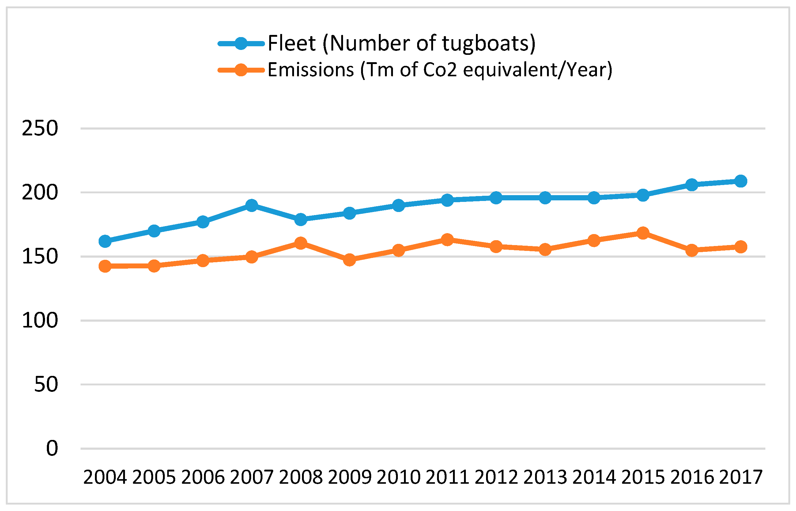
3.1. Emissions of the Spanish Tugboat Fleet

In the period analyzed (2004–2017), the Spanish tugboat fleet increased by 29.01% in number, while the emissions increased by 42.54% in Tm of CO2 equivalent. The average rate of the emissions measured ranged from 143 to 168 Tm of CO2 equivalent (see Figure 3). The x-axis shows the CO2 emissions and the y-axis shows the years in which the emissions occur.
Figure 4 shows the distribution of the emissions of greenhouse gases of the Spanish tugboat fleet among the ports of the different regions for the period analyzed (x-axis). The fleets of the regions of Galicia, Canary Islands, Community of Valencia and Andalusia (y-axis) have the highest values, with average values of over 3000 Tm of CO2 equivalent.
By groups of age (A), until the year 2015, the fleet of ships under 10 years old was the one that emitted the highest quantity of Tm of CO2 equivalent. After 2015, however, it is the fleet of tugboats of over 15 years of age that produces the highest quantity of greenhouse gas emissions in the Spanish ports. In Figure 5, the x-axis shows the emissions of tons of CO2 and the y-axis shows the years.
By groups of size (measured in GT), the fleet of tugboats of between 300 and 400 GT was the one that produced the most emissions for the period analyzed, except for the year 2017, when the tugboats of over 400 GT were the ones that polluted the most (see Figure 6) the x-axis shows the emissions of tons of CO2 and the y-axis show the years.
Regarding the power groups (measured in kW), the tugboats with power of between 2000 and 4000 kW were the ones that produced the largest emissions of greenhouse gases in the period analyzed. In Figure 7, the x-axis shows the emissions of tons of CO2 and the y-axis shows the years.

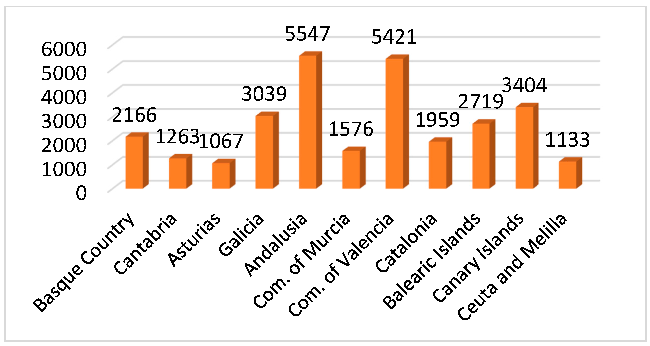
3.2. Participation in the Carbon Footprint

Since 2008, the National Institute of Statistics of Spain (INE) has published the Records of Emissions into the Atmosphere by Activity Branches (CNAE 2009). At present, the series covers up to the year 2015. Branch 50 presents the emissions generated by marine transport and transport in inner navigable waters. The quantities are expressed in thousands of Tm of CO2 Eq. We have available then the carbon footprint of the whole Spanish marine transport sector, so that by comparing these emissions with those produced by the tugboat sector, we can establish the contribution of this sector to the carbon footprint of the country’s marine transport sector (Table 3).
In the period analyzed (2008–2015), there was an increase in both the emissions of greenhouse gases of the Spanish tugboat fleet and in its contribution to the carbon footprint of the Spanish marine transport sector, even though the total emissions of the sector fell.

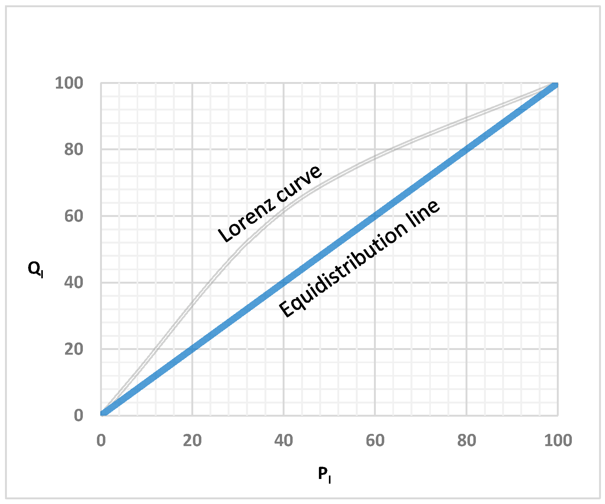
3.3. Concentration Indices of the Greenhouse Gas Emissions Lorenz Curves of the Spanish Tugboat Fleet

The concentration indices of the greenhouse gas emissions of the tugboat fleet operating in Spanish ports in the period 2004–2017 is shown in Table 4. The indices have been classified by regions (autonomous communities), by age, and by size, measured in GT.
By region (autonomous community), the concentration of the emissions of greenhouse gases caused by the activity of the Spanish tugboat fleet, measured in Tm of CO2 equivalent in the period analyzed (2004–2017), increased by 14.26%, as shown in Table 3. In the period before the economic recession (2004–2007), the concentration decreased by 18.7%. During the recession (2008–2013), the concentration of gases increased by 61.15%. After the economic recession (2014–2017), the concentration of gases decreased again by 3.29%.
Figure 8 shows the Lorenz curves for the years 2004, 2010 and 2017, where it can be seen that in the last year, the curve distances itself from the diagonal, showing the increase in the concentration indicated in the period.
In 2017, 38.28% of the tugboat fleet emitted 57.02% of the CO2 equivalent. These were the tugboats that operate in the ports of the Balearic Islands, Murcia, Ceuta and Melilla, Cantabria, Valencia, and the Canary Islands (see Figure 2). On the other hand, 61.72% of the remaining fleet operating in the regions of Andalusia, Catalonia, the Basque Country, Galicia and Asturias emitted 42.98% of the greenhouse gases.
By age in the period analyzed (2004–2017), the concentration of greenhouse gas emissions fell. In the year 2017, the tugboat fleet of over 15 years of age that made up 66.51% of the total of the fleet emitted 56.39% of the total of the greenhouse gas emissions of the fleet (see Figure 9).
By size, measured in GT, in the period analyzed (2004–2017), the concentration of greenhouse gas emissions fell. In the year 2017, the part of the fleet made up of tugboats of less than 400 GT, which makes up 49.76% of the fleet, emitted 65.78% of the total (see Figure 10).

4. Discussion

In the present work, two different types of methodology have been used in a complementary manner: one to estimate emissions and the other to determine their degree of concentration. In the case of the bottom-up methodology for estimating emissions, the procedure most widely used in the maritime sector has been chosen. In the case of the concentration analysis, the Gini indices have been chosen, as these are widely used in work on health indicators.
This is the methodology used by the International Maritime Organization (IMO). Controversy surrounding this methodology occurred during 2009 and 2017 [72,73,74,75] of the period analyzed in technological, legal and socioeconomic contexts. These references have been fully formalized in Section 2.1 of the introduction.
Although both methodologies have been shown to be effective for the purposes of this work, this does not imply that other methodologies may not be used either to estimate emissions or to determine their concentration (for example, the Theil indices).
Although reference is made to the Spanish maritime port sector (all commercial maritime ports), it has been decided to undertake a regional analysis, in order to present a more global view of the sector. This means that all of the maritime-commercial ports of each region are grouped together, even though their size and level of activity may be different.
The concentration indices have been estimated for the entire period analyzed (2004–2017). However, the Lorenz curves have only been formalized for 3 years. The aim is to show more clearly the evolution of the concentration in the three bounded periods, since each year is identified with a period.
The carbon footprint of the Spanish tugboat fleet has been obtained for the period 2008–2015, since these are the only years for which there are published data on emissions from the total Spanish fleet of merchant ships.

5. Conclusions

a.
The methodologies used in a complementary way for the estimation of greenhouse gas emissions (bottom-up) and the analysis of their concentration for different groups of variables have proven to be efficient in the present analysis and could be applied in other works on other sectors of the fleet and different spatial areas.
b.
In the period analyzed (2007–2017), the emissions produced by the activity of the Spanish ports tugboat fleet increased by 15.53% more than the fleet as a whole did.
c.
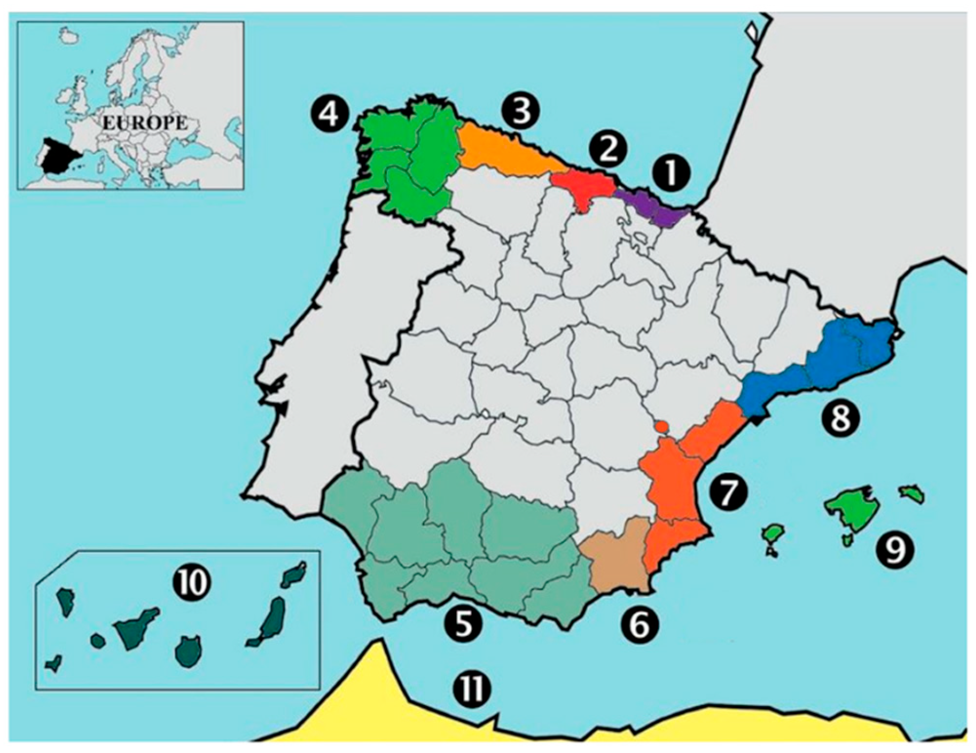
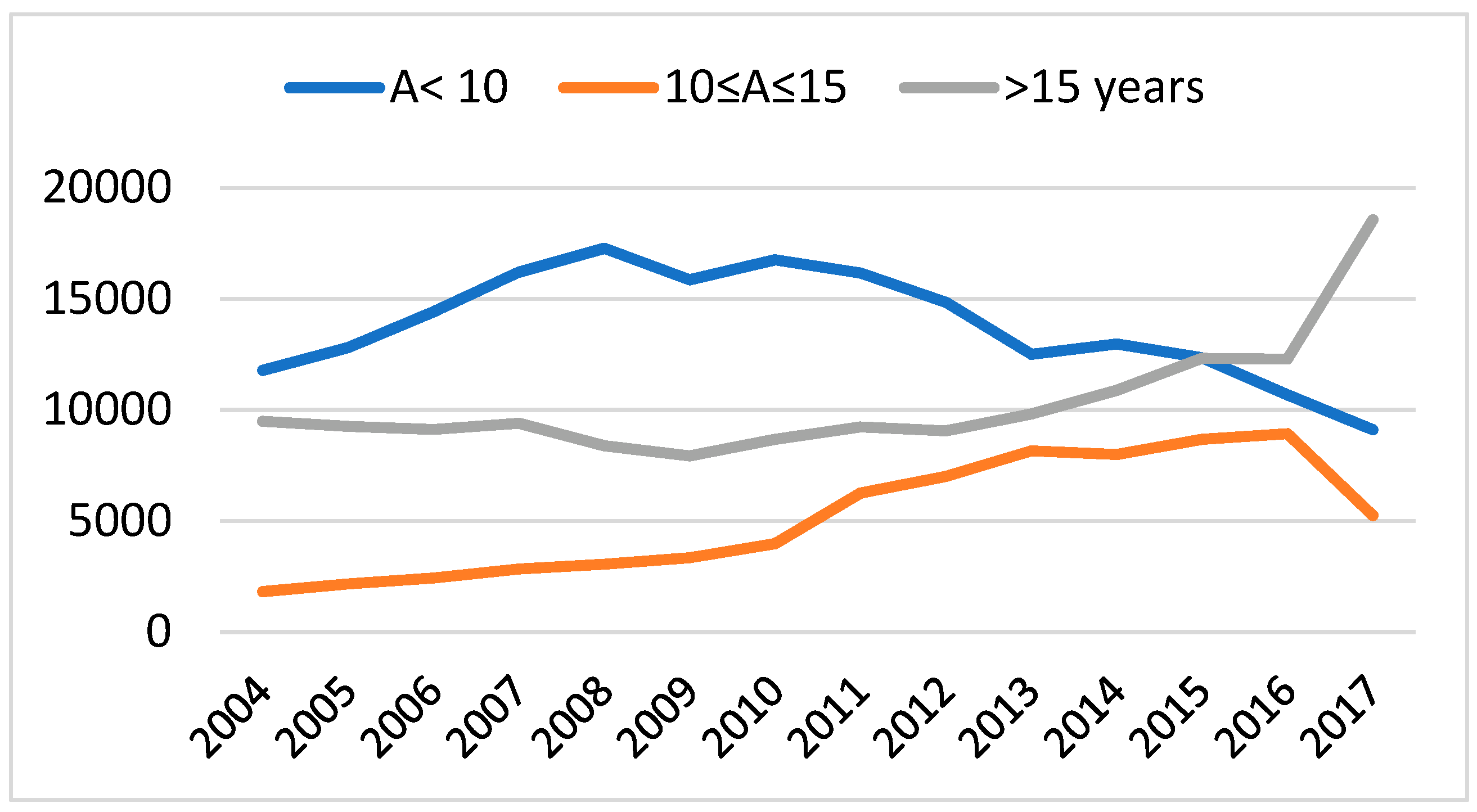
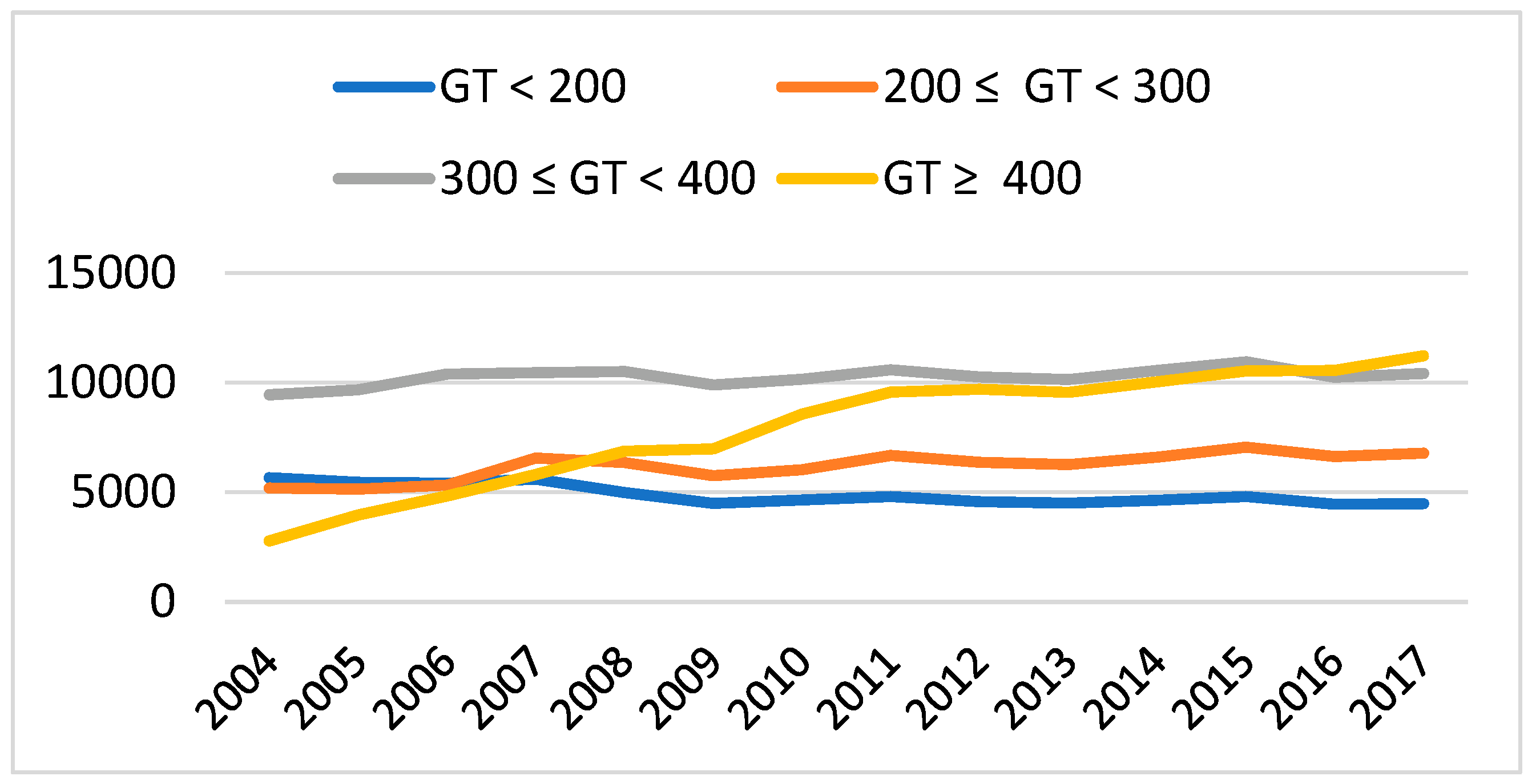
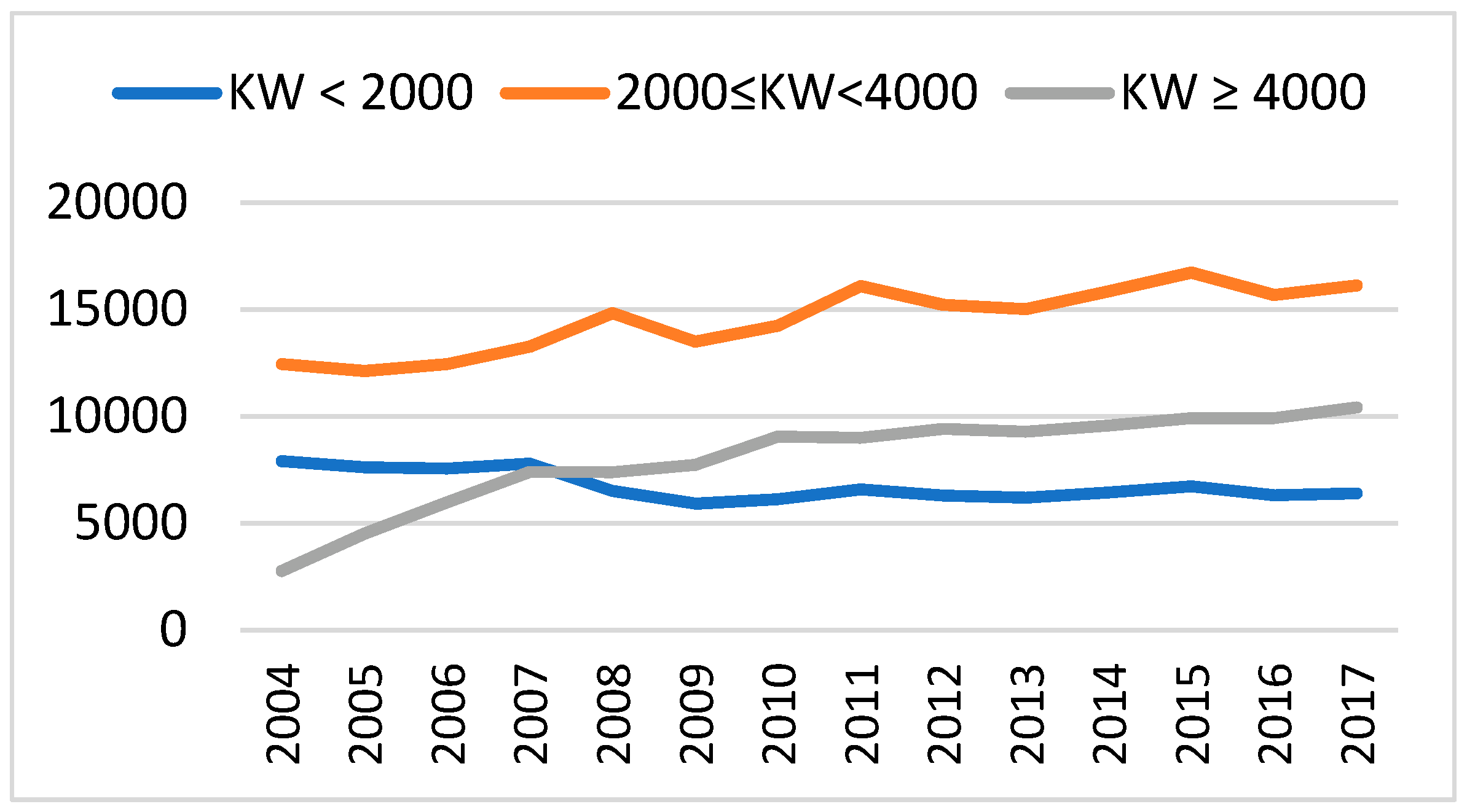
The profile of the port tugboat of the Spanish fleet that pollutes the most greenhouse gases in the period analyzed would be a tugboat under 15 years old, weight between 300 and 400 GT, engine power between 2000 and 4000 kW, and one that operates in the ports of the autonomous community (region) of Andalusia.
d.
In the period 2008–2015, the carbon footprint of the Spanish fleet of port tugboats increased, while that of the total sector of Spanish maritime transport decreased. This means that in this period, the participation of the Spanish sector of port tugboats in the total maritime transport increased, going from 0.66% in 2008 to 2.24% in 2015.
e.
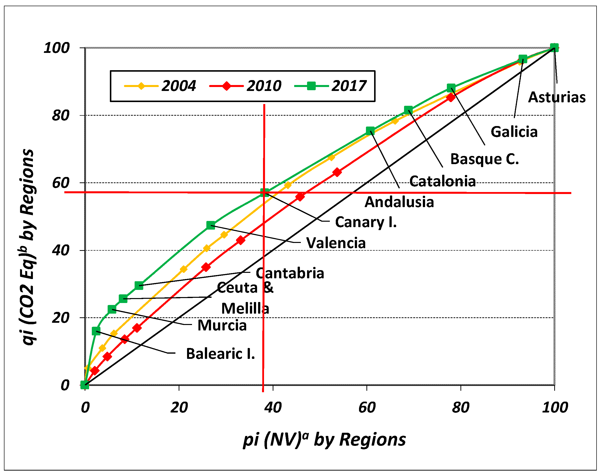
In the period analyzed (2004–2017), the results obtained from the estimation of the Gini indices allow a relationship to be established for Spain between its level of economic activity and the degree of concentration of emissions from its fleet of port tugboats. In periods of crisis (economic recession), port activity is reduced and tends to concentrate more in the most efficient ports; therefore, the emissions of the tugs that operate in those ports also tend to concentrate more. In periods of growth (economic expansion), port activity increases and a greater number of ports are used to avoid congestion, meaning that the fleets operating in those ports are more spread out and the emissions produced by their activity are also more widely distributed.
f.
In the period analyzed (2004–2017), the concentration of emissions of the Spanish tugboat fleet increased if we look at its distribution by region and decreased if we look at its distribution by age and size. This is due to the fact that tugboat activity was very different by region; however, its characteristics relative to age and size evolved more homogeneously.

Author Contributions

Conceptualization, A.O.-P. and E.D.-R.-N.; formal analysis, A.H.M., M.A.G. and A.-I.L.-D.; investigation; writing—original draft preparation A.O.-P. and E.D.-R.-N.; writing—review and editing, A.H.M., M.A.G. and A.-I.L.-D. All authors have read and agreed to the published version of the manuscript.

Funding

This research received no external funding.

Institutional Review Board Statement

Not applicable.

Informed Consent Statement

Not applicable.

Data Availability Statement

Not applicable.

Conflicts of Interest

The authors declare no conflict of interest.

References

  1. Naciones Unidas. United Nations Framework Convention on Climate Change. 1992. Available online: https://digitallibrary.un.org/record/180257?ln=es (accessed on 10 November 2022).
  2. Cmnucc, P.K. United Nations Framework Convention on Climate Change; United Nations: New York, NY, USA, 1998. [Google Scholar]
  3. Kraska, J. Particularly Sensitive Sea Areas and the Law of the Sea; Center for Oceans Law and Policy: Charlottesville, VA, USA, 2009. [Google Scholar]
  4. Pak, M. A Study on the International Instruments of Air Pollution Prevention from Ships. Marit. Law Rev. 2009, 21, 1–36. [Google Scholar]
  5. Nicholson, E.; Henneberry, C. Adopting the model: How government vessels can benefit from commercial sustainability. Mar. Technol. 2011, 48, 48–53. [Google Scholar]
  6. Wan Dahalan, W.S.A.; Zainol, Z.A.; Yaa’kub, N.I.; Kassim, N.M. Corporate social responsibility (CSR) from shipping companies in the straits of Malacca and Singapore. Int. J. Bus. Soc. 2012, 13, 197–208. [Google Scholar]
  7. Hermida-Castro, M.J.; Hermida-Castro, D.; Orosa, J.A.; Silva-Costas, M.M. Passenger ships inspection in Spanish ports navigation. J. Marit. Res. 2014, 10, 3–6. [Google Scholar]
  8. Cogliolo, A. Sustainable shipping green innovation for the marine industry. Rend. Lincei 2015, 26, 65–72. [Google Scholar] [CrossRef]
  9. Tanaka, Y. Regulation of greenhouse gas emissions from international shipping and jurisdiction of states. Rev. Eur. Comp. Int. Environ. Law 2016, 25, 333–346. [Google Scholar] [CrossRef]
  10. Jin, H.-Z.; Su, X.-Y.; Yu, A.-C.; Lin, F. Design of automatic mooring positioning system based on mooring line switch. Dianji Yu Kongzhi Xuebao/Electr. Mach. Control 2014, 18, 93–98. [Google Scholar]
  11. Kanifolskyi, O.O. EEDI (energy efficiency design index) for small ships of the transitional mode. Trans. R. Inst. Nav. Archit. Part B Int. J. Small Craft Technol. 2014, 156, 39–41. [Google Scholar] [CrossRef]
  12. Zhu, L.; Jessen, H.; Zhang, M. The Way Forward for Hong Kong to Combat Vessel Source Emissions in the Pearl River Delta Region. Ocean Dev. Int. Law 2015, 46, 208–224. [Google Scholar] [CrossRef]
  13. George, M.; Osman, A.S.S.; Hussin, H.; George, A.R. Protecting the Malacca and Singapore Straits from Ships’ Atmospheric Emissions through the Implementation of MARPOL Annex VI. Int. J. Mar. Coast. Law 2017, 32, 95–137. [Google Scholar] [CrossRef]
  14. Myoung-Hwan, K.I.M. Performance and Safety Analysis of Marine Solid Oxide Fuel Cell Power System. J. Korean Soc. Mar. Eng. 2009, 33, 233–243. [Google Scholar]
  15. Yang, B.; Sun, P.; Huang, L.; Song, D. The Prospective Analysis of Marine Dual Fuel Engine Application Based on Emission and Energy Efficiency. Adv. Energy Sci. Technol. 2013, 291, 1975–1980. [Google Scholar]
  16. Díaz-de-Baldasano, M.C.; Mateos, F.J.; Núñez-Rivas, L.R.; Leo, T.J. Conceptual design of offshore platform supply vessel based on hybrid diesel generator-fuel cell power plant. Appl. Energy 2014, 116, 91–100. [Google Scholar] [CrossRef] [Green Version]
  17. Ehara, Y.; Osako, A.; Zukeran, A.; Kawakami, K.; Inui, T. Diesel PM collection for marine emission using hole-type electrostatic precipitators. WIT Trans. Ecol. Environ. 2014, 183, 145–155. [Google Scholar] [CrossRef] [Green Version]
  18. Wang, S.; Notteboom, T. The Adoption of Liquefied Natural Gas as a Ship Fuel: A Systematic Review of Perspectives and Challenges. Transp. Rev. 2014, 34, 749–774. [Google Scholar] [CrossRef]
  19. Zhou, S.; Zhang, C. Marine SCR Technology’s Development and Prospects. Mech. Sci. Eng. IV 2014, 472, 909–916. [Google Scholar]
  20. Ekanem Attah, E.; Bucknall, R. An analysis of the energy efficiency of LNG ships powering options using the EEDI. Ocean Eng. 2015, 110, 62–74. [Google Scholar] [CrossRef]
  21. Kim, J.-H.; Park, H.-W. Basic study of residual marine fuels quality. J. Korean Soc. Mar. Eng. 2016, 40, 362–368. [Google Scholar] [CrossRef]
  22. Fernandez, I.A.; Gomez, M.R.; Gomez, J.R.; Insua, A.A.B. Review of propulsion systems on LNG carriers. Renew. Sustain. Energy Rev. 2017, 67, 1395–1411. [Google Scholar] [CrossRef]
  23. Ling-Chin, J.; Roskilly, A.P. Investigating a conventional and retrofit power plant on-board a Roll-on/Roll-off cargo ship from a sustainability perspective—A life cycle assessment case study. Energy Convers. Manag. 2016, 117, 305–318. [Google Scholar] [CrossRef] [Green Version]
  24. Geng, P.; Mao, H.; Zhang, Y.; Wei, L.; You, K.; Ju, J.; Chen, T. Combustion characteristics and NOx emissions of a waste cooking oil biodiesel blend in a marine auxiliary diesel engine. Appl. Therm. Eng. 2017, 115, 947–954. [Google Scholar] [CrossRef]
  25. Yoon, Y.-N.; Choi, Y. Feasibility Study of a Shipboard Sewage Treatment Plant (Sequencing Batch Reactor and Membrane Bioreactor) in Accordance with MARPOL 73/78, Focusing Mostly on Nutrients (T-N and T-P). J. Environ. Sci. Int. 2016, 25, 1233–1239. [Google Scholar] [CrossRef]
  26. Fet, A.M.; Schau, E.M.; Haskins, C. A framework for environmental analyses of fish food production systems based on systems engineering principles. Syst. Eng. 2010, 13, 109–118. [Google Scholar] [CrossRef]
  27. Luttenberger, L.R.; Ancic, I.; Šestan, E.A. The Viability of Short-Sea Shipping in Croatia. Brodogradnja 2013, 64, 472–481. Available online: https://www.scopus.com/inward/record.uri?eid=2-s2.0-84904963812&partnerID=40&md5=24103fb9b159154c7f9cd56576294eb1 (accessed on 20 January 2021).
  28. Schinas, O.; Stefanakos, C. Selecting technologies towards compliance with MARPOL Annex VI: The perspective of operators. Transp. Res. Part D Transp. Environ. 2014, 28, 28–40. [Google Scholar] [CrossRef]
  29. Panasiuk, I.; Turkina, L. The evaluation of investments efficiency of SOx scrubber installation. Transp. Res. Part D Transp. Environ. 2015, 40, 87–96. [Google Scholar] [CrossRef]
  30. Makkonen, T.; Repka, S. The innovation inducement impact of environmental regulations on maritime transport: A literature review. Int. J. Innov. Sustain. Dev. 2016, 10, 69–86. [Google Scholar] [CrossRef]
  31. Rutkowski, G. Study of New Generation LNG Duel Fuel Marine Propulsion Green Technologies. Transnav-Int. J. Mar. Navig. Saf. Sea Transp. 2016, 10, 641–645. [Google Scholar] [CrossRef] [Green Version]
  32. Doudnikoff, M.; Gouvernal, E.; Lacoste, R. The reduction of ship-based emissions: Aggregated impact on costs and emissions for North Europe-East Asia liner services. Int. J. Shipp. Transp. Logist. 2014, 6, 213–233. [Google Scholar] [CrossRef]
  33. Holmgren, J.; Nikopoulou, Z.; Ramstedt, L.; Woxenius, J. Modelling modal choice effects of regulation on low-sulphur marine fuels in Northern Europe. Transp. Res. Part D Transp. Environ. 2014, 28, 62–73. [Google Scholar] [CrossRef]
  34. Sys, C.; Vanelslander, T.; Adriaenssens, M.; Van Rillaer, I. International emission regulation in sea transport: Economic feasibility and impact. Transp. Res. Part D Transp. Environ. 2014, 45, 139–151. [Google Scholar] [CrossRef]
  35. Vleugel, J.M.; Bal, F. Cleaner air in seaport container terminals: Assessing fuel(s). WIT Trans. Ecol. Environ. 2014, 181, 25–36. [Google Scholar] [CrossRef] [Green Version]
  36. Adamkiewicz, A.; Cydejko, J. An analysis of LNG carrier propulsion systems in the aspect of satisfying emission control area requirements. Rynek Energii 2015, 118, 80–86. [Google Scholar]
  37. Lindstad, H.E.; Eskeland, G.S. Environmental regulations in shipping: Policies leaning towards globalization of scrubbers deserve scrutiny. Transp. Res. Part D Transp. Environ. 2016, 47, 67–76. [Google Scholar] [CrossRef] [Green Version]
  38. Peksen, D.Y.; Alkan, G.; Bayar, S.; Yildiz, M.; Elmas, G. Lng as Ship Fuel for Sox Emission Reduction Target in the Sea of Marmara. Fresenius Environ. Bull. 2016, 25, 1406–1419. [Google Scholar]
  39. Schinas, O.; Butler, M. Feasibility and commercial considerations of LNG-fueled ships. Ocean Eng. 2016, 122, 84–96. [Google Scholar] [CrossRef]
  40. Shi, Y. Reducing greenhouse gas emissions from international shipping: Is it time to consider market-based measures? Mar. Policy 2016, 64, 123–134. [Google Scholar] [CrossRef]
  41. Nikopoulou, Z. Incremental costs for reduction of air pollution from ships: A case study on North European emission control area. Marit. Policy Manag. 2017, 44, 1056–1077. [Google Scholar] [CrossRef]
  42. Teo, T. Energy efficiency for OSVs. Oil Gas J. 2012, 110, 40–43. [Google Scholar]
  43. Yang, Z.L.; Zhang, D.; Caglayan, O.; Jenkinson, I.D.; Bonsall, S.; Wang, J.; Huang, M.; Yan, X.P. Selection of techniques for reducing shipping NOx and SOx emissions. Transp. Res. Part D Transp. Environ. 2012, 17, 478–486. [Google Scholar] [CrossRef]
  44. Calleya, J.; Pawling, R.; Greig, A. Ship impact model for technical assessment and selection of Carbon dioxide Reducing Technologies (CRTs). Ocean Eng. 2015, 97, 82–89. [Google Scholar] [CrossRef] [Green Version]
  45. Sherbaz, S.; Maqsood, A.; Khan, J. Machinery options for green ship. J. Eng. Sci. Technol. Rev. 2015, 8, 169–173. [Google Scholar] [CrossRef]
  46. Fu, S.; Yan, X.; Zhang, D.; Li, C.; Zio, E. Framework for the quantitative assessment of the risk of leakage from LNG-fueled vessels by an event tree-CFD. J. Loss Prev. Process Ind. 2016, 43, 42–52. [Google Scholar] [CrossRef] [Green Version]
  47. Jankowski, S. An international platform for cooperation on liquefied natural gas (LNG)—A report on the MarTech LNG project. Sci. J. Marit. Univ. Szczec.-Zesz. Nauk. Akad. Mor. Szczec. 2016, 46, 29–35. [Google Scholar] [CrossRef]
  48. Kitada, M.; Dalaklis, D.; Drewniak, M.; Olcer, A.; Ballini, F. Exploring the frontiers of maritime energy management research. In Global Perspectives in MET: Towards Sustainable, Green and Integrated Maritime Transport; Nikola Vaptsarov Naval Academy: Varna, Bulgaria, 2017; pp. 481–490. [Google Scholar]
  49. Bencs, L.; Horemans, B.; Buczyńska, A.J.; Van Grieken, R. Uneven distribution of inorganic pollutants in marine air originating from ocean-going ships. Environ. Pollut. 2017, 222, 226–233. [Google Scholar] [CrossRef]
  50. Ölçer, A.I.; Ballini, F.; Kitada, M.; Dalaklis, D. Development of a Holistic Maritime Energy Management Programme at the Postgraduate Level: The Case of WMU; World Maritime University: Malmö, Sweden, 2017. [Google Scholar]
  51. Cappa, C.D.; Williams, E.J.; Lack, D.A.; Buffaloe, G.M.; Coffman, D.; Hayden, K.L.; Herndon, S.C.; Lerner, B.M.; Li, S.-M.; Massoli, P.; et al. A case study into the measurement of ship emissions from plume intercepts of the NOAA ship Miller Freeman. Atmos. Chem. Phys. 2014, 14, 1337–1352. [Google Scholar] [CrossRef]
  52. Davies, M. Ship emissions from australian ports. WIT Trans. Ecol. Environ. 2014, 183, 327–337. [Google Scholar] [CrossRef] [Green Version]
  53. Kattner, L.; Mathieu-Üffing, B.; Burrows, J.P.; Richter, A.; Schmolke, S.; Seyler, A.; Wittrock, F. Monitoring compliance with sulfur content regulations of shipping fuel by in situ measurements of ship emissions. Atmos. Chem. Phys. 2015, 15, 10087–10092. [Google Scholar] [CrossRef] [Green Version]
  54. Buccolieri, R.; Cesari, R.; Dinoi, A.; Maurizi, A.; Tampieri, F.; Di Sabatino, S. Impact of ship emissions on local air quality in a Mediterranean city’s harbour after the European sulphur directive. Int. J. Environ. Pollut. 2016, 59, 30–42. [Google Scholar] [CrossRef]
  55. Dogrul, A.; Ozden, Y.A.; Celik, F. A Numerical Investigation of SO2 Emission in the Strait of Istanbul. Fresenius Environ. Bull. 2016, 25, 5795–5803. [Google Scholar]
  56. Kilic, A. Establishment of NOx measurement and certification system for small ships. Trans. R. Inst. Nav. Archit. Part A Int. J. Marit. Eng. 2016, 158, A131–A138. [Google Scholar] [CrossRef]
  57. Xing, H.; Duan, S.-L.; Huang, L.-Z.; Han, Z.-T.; Liu, Q.-A. Testbed-based exhaust emission factors for marine diesel engines in China. Huanjing Kexue/Environ. Sci. 2016, 37, 3750–3757. [Google Scholar] [CrossRef]
  58. Jalkanen, J.P.; Johansson, L.; Kukkonen, J. A comprehensive inventory of ship traffic exhaust emissions in the European sea areas in 2011. Atmos. Chem. Phys. 2016, 16, 71–84. [Google Scholar] [CrossRef]
  59. Cheng, H.-M.; Liu, C.; Hou, P.-X. Field emission from carbon nanotubes. In Nanomaterials Handbook, 2nd ed.; CRC Press: Boca Raton, FL, USA, 2017; pp. 255–272. [Google Scholar]
  60. Demarco, N. Recession tugs at marine lubes. Lubes-n-Greases 2009, 15, 25–27. [Google Scholar]
  61. Papson, A.; Hartley, S.; Browning, L. Cost-Effectiveness of Five Emission Reduction Strategies for Inland River Tugs and Towboats. Transp. Res. Rec. 2010, 2166, 109–115. [Google Scholar] [CrossRef]
  62. Ayre, L.S.; Johnson, D.R.; Clark, N.N.; England, J.A.; Atkinson, R.J.; McKain, D.L., Jr.; Ralston, B.A.; Balon, T.H., Jr.; Moynihan, P.J. Novel NOx Emission Reduction Technology for Diesel Marine Engines. In Proceedings of the Asme Internal Combustion Engine Division Fall Technical Conference (ICEF), Morgantown, WV, USA, 2–5 October 2011; Amer Soc Mechanical Engineers: New York, NY, USA, 2011; pp. 703–710. [Google Scholar]
  63. Murphy, A.J.; Weston, S.J.; Young, R.J. Reducing fuel usage and CO2 emissions from tug boat fleets: Sea trials and theoretical modelling. Trans. R. Inst. Nav. Archit. Part A Int. J. Marit. Eng. 2012, 154, 31–41. [Google Scholar] [CrossRef]
  64. Van Den Hanenberg, G. Tug goes green Partnering up for lower fuel consumption through increased sustainability. Marit. By Holl. 2012, 61, 14–16. [Google Scholar]
  65. Niemi, M. Propulsor evolution. Mar. Technol. 2013, 50, 44–47. [Google Scholar]
  66. Sciberras, E.A.; Zahawi, B.; Atkinson, D.J.; Juandó, A. Electric auxiliary propulsion for improved fuel efficiency and reduced emissions. Proc. Inst. Mech. Eng. Part M J. Eng. Marit. Environ. 2015, 229, 36–44. [Google Scholar] [CrossRef] [Green Version]
  67. Trodden, D.G.; Murphy, A.J.; Pazouki, K.; Sargeant, J. Fuel usage data analysis for efficient shipping operations. Ocean Eng. 2015, 110, 75–84. [Google Scholar] [CrossRef] [Green Version]
  68. Faturachman, A.D.; Febrian, B.S.; Novita, C.T.D.; Djaeni, D.A.; Oktavia, E.E.T.A. Main Engine Fuel Oil Consumption by Using Flow Meter on Tug Boat. Int. J. Mech. 2016, 10, 7–13. Available online: https://www.scopus.com/inward/record.uri?eid=2-s2.0-85000843755&partnerID=40&md5=bdd9dd88d1443a1e93b14dbc34002f76 (accessed on 20 April 2015).
  69. Gysel, N.R.; Russell, R.L.; Welch, W.A.; en Cocker, D.R., III. Impact of Aftertreatment Technologies on the in-Use Gaseous and Particulate Matter Emissions from a Tugboat. Energy Fuels 2016, 30, 684–689. [Google Scholar] [CrossRef] [Green Version]
  70. Lim, S.; Pazouki, K.; Murphy, A.J. Holistic Energy Mapping Methodology for Reduced Fuel Consumption and Emissions. In Proceedings of the ASME 2017 36th International Conference on Ocean, Offshore and Arctic Engineering, Trondheim, Norway, 25–30 July 2017. [Google Scholar]
  71. Buhaug, Ø.; Corbett, J.J.; Endresen, Ø.; Eyring, V.; Faber, J.; Hanayama, S.; Lee, D.S.; Lee, D.; Lindstad, H.; Markowska, A.Z.; et al. Second IMO GHG Study 2009; International Maritime Organization: London, UK, 2009. [Google Scholar]
  72. Oria Chaveli, J.M. Emisiones Contaminantes a la Atmósfera del Transporte Marítimo en el Puerto de Santander; Universidad de Cantabria: Santander, Spain, 2016. [Google Scholar]
  73. Eyring, V.; Isaksen, I.S.A.; Berntsen, T.; Collins, W.J.; Corbett, J.J.; Endresen, O.; Grainger, R.G.; Moldanova, J.; Schlager, H.; Stevenson, D.S. Transport impacts on atmosphere and climate: Shipping. Atmos. Environ. 2010, 44, 4735–4771. [Google Scholar] [CrossRef]
  74. Miola, A.; Ciuffo, B.; Giovine, E.; Marra, M. Regulating Air Emissions from Ships: The State of the Art on Methodologies, Technologies and Policy Options; European Commission: Brussels, Belgium, 2010. [Google Scholar]
  75. Chevron Richmond Long Wharf Shipping Emissions Model—PDF Free Download. Available online: https://docplayer.net/46987643-Chevron-richmond-long-wharf-shipping-emissions-model.html (accessed on 19 May 2021).
  76. Sen, A. On Economic Inequality; Oxford University Press: Oxford, UK, 1973. [Google Scholar]
Figure 1. Lorenz curve. Source: authors. Pi = accumulated percentage (%) of the value of the population variable analyzed (X) and Qi = accumulated percentage (%) of the variable of the emission of CO2 equivalent (FX) of the population analyzed (X).
Atmosphere 13 02109 g001
Figure 2. Distribution of coastal regions of Spain. Basque Country (1), Cantabria (2), Asturias (3), Galicia (4), Andalusia (5), Com. Murcia (6), Com. Valencia (7), Catalonia (8), Balearic Islands (9), Canary Islands (10) and Ceuta and Melilla (11). Source: Authors.
Atmosphere 13 02109 g002
Figure 3. Evolution of the Spanish ports tugboat fleet and emissions measured. Source: Authors.
Atmosphere 13 02109 g003
Figure 4. Distribution of fleet emissions by coastal regions in Spain. Source: Authors.
Atmosphere 13 02109 g004
Figure 5. Evolution of emissions of Spanish tugboat fleet, by groups of age. Source: Authors.
Atmosphere 13 02109 g005
Figure 6. Evolution of emissions of the Spanish tugboat fleet, by groups of size, measured in GT. Source: authors.
Atmosphere 13 02109 g006
Figure 7. Evolution of emissions of Spanish tugboat fleet, by groups of power, measured in kW. Source: Authors.
Atmosphere 13 02109 g007
Figure 8. Lorenz curves of emissions of CO2 equivalent of the tugboats in Spanish ports by region. Source: authors. a = % accumulated number of tugboats by regions; b = % accumulated emissions of CO2 equivalent by region.
Atmosphere 13 02109 g008
Figure 9. Lorenz curves of the greenhouse gas emissions of the Spanish tugboat fleet by age. Source: Authors. a = accumulated percentage of tugboats by age; b = accumulated percentage of emissions of CO2 equivalent by age.
Atmosphere 13 02109 g009
Figure 10. Lorenz curves of greenhouse gas emissions of the Spanish tugboat fleet by size (GT). Source: Authors. a = accumulated percentage of tugboats by GT; b =accumulated percentage of emissions of CO2 equivalent by GT.
Atmosphere 13 02109 g010
Table 1. Variables used in the construction of the concentration indices.
G a X ( t ) b F X ( t ) c
N V ( t ) G T ( t ) K W ( t ) C O 2 E ( t )
1 N V 1 ( t ) G T 1 ( t ) K W 1 ( t ) C O 2 E 1 ( t )
i N V i ( t ) G T i ( t ) K W i ( t ) C O 2 E i ( t )
k N V k ( t ) G T k ( t ) K W k ( t ) C O 2 E k ( t )
Total i = 1 k N V i ( t ) i = 1 k G T i ( t ) i = 1 k K W i ( t ) i = 1 k C O 2 E i ( t )
Source: Authors. a = groups of variables. In the present work, this grouping is made according to regions, age, size (GT) and power (KW). b = population variable analyzed of the fleet i in the period t (NV = number of tugboats; GT = size in gross tons; kW = installed power in kW). c = Variable of gas emissions (CO2E = greenhouse gases).
Table 2. Average data of the 14 years analyzed (2004–2017).
Coastal Autonomous CommunitiesVesselsGTKW
1BASQUE COUNTRY15484937,457
2CANTABRIA4159217,338
3ASTURIAS13460032,366
4GALICIA2811,45378,745
5ANDALUSIA4612,470101,342
6COM MURCIA7459630,514
7COM VALENCIANA29822775,943
8CATALONIA14457745,710
9BALEARIC ISLANDS5157110,640
10CANARY ISLAND24661158,703
11CEUTA AND MELILLA510657673
Source: Authors.
Table 3. Carbon footprint of the Spanish ports tugboat fleet and its contribution to the carbon footprint of the Spanish marine transport sector (2008–2015).
YearFPMT aFPT b(%)FPMT c
20084343.9028.720.66%
20093636.6027.130.75%
20103465.3029.420.85%
20112739.4031.661.16%
20122833.2030.911.09%
20131716.6030.491.78%
20141141.6031.852.79%
20151487.7033.362.24%
Source: authors. a carbon footprint of the Spanish marine transport sector measured in thousands of Tm of CO2 Eq; b carbon footprint of the Spanish tugboat fleet measured in thousands of Tm of CO2 Eq; c contribution of emissions of the Spanish tugboat fleet to the carbon footprint of the Spanish marine transport sector.
Table 4. Concentration indices of the greenhouse gas emissions of the Spanish tugboat fleet.
PERIODYearFGIREGION aFGIAYE bFGIGT c
BEFORE
ECONOMIC
RECESSION
OriginalANTES DE LA RECESIÓN ECONÓMICA
2004−0.324−0.535−0.449
2005−0.295−0.534−0.458
2006−0.279−0.533−0.465
2007−0.263−0.444−0.429
ECONOMIC RECESSION2008−0.213−0.355−0.359
2009−0.203−0.359−0.359
2010−0.186−0.345−0.345
2011−0.299−0.367−0.329
2012−0.327−0.377−0.330
2013−0.342−0.367−0.330
AFTER
ECONOMIC
RECESSION
2014−0.383−0.392−0.334
2015−0.398−0.395−0.327
2016−0.351−0.331−0.297
2017−0.370−0.307−0.293
Source: authors. a GINI FGIr concentration indices of greenhouse gas emissions of Spanish tugboat fleet by region; b GINI FGIy concentration indices of greenhouse gas emissions of Spanish tugboat fleet by age; c GINI FGIgt concentration indices of greenhouse gas emissions of Spanish tugboat fleet by size (GT).
Publisher’s Note: MDPI stays neutral with regard to jurisdictional claims in published maps and institutional affiliations.

