Wind Characteristics in the Surface Layer on Different Underlying Surfaces in High Altitude Areas of Central and Western China

Abstract

To explore the influence of complex terrain on wind characteristics of the surface layer and to better develop and utilize wind energy resources of high-altitude regions in central and western China, two typical topographies: the Qiaodi Village in Sichuan (in western China, site 1) and the Nanhua Mountain in Shanxi (in central China, site 2), were selected for this study. The diurnal and monthly variations of the atmospheric stability were contrasted at the two sites, according to the Obukhov length calculated by the eddy covariance data. The energy exchange process between complex underlying surfaces and the atmospheric boundary layer can be reflected to a certain extent by investigating the diurnal variation differences of the turbulent fluxes at the two sites. The results show that: (1) the dominant boundary layer at site 1 during nighttime is the neutral boundary layer, while at site 2 it is the stable; (2) the horizontal wind speed at 10 m above the ground is the highest (lowest) in the neutral (unstable) boundary layer at site 1, while it is the highest (lowest) in the neutral and weak-unstable (stable) boundary layer at site 2, and (3) the momentum flux, sensible heat flux, and latent heat flux all show unimodal diurnal characteristics. There is a 1 h lag in the flux peak at site 1 compared to site 2.

1. Introduction

China’s topography is high in the west and low in the east, presenting a step-like distribution, and the typical terrain in the central and western regions are mountains and plateau basins. According to the internationally accepted altitude classification standard above the sea level: 1500–3500 m is high altitude; 3500–5500 m is ultra-high altitude; and above 5500 m is extremely high altitude [1]. Most of the mountainous areas in central and western China belong to high-altitude areas where wind characteristics of the surface layer are quite different from the vast flat areas in eastern China [2]. It is difficult to observe and evaluate the wind power in these mountainous areas, both for technology and for work processing. Therefore, in order to explore the influence of complex terrain on wind characteristics of the surface layer and to better develop and utilize wind energy resources of high-altitude regions in central and western China, it is necessary to carry out research to discover the wind characteristics of the surface layer over some typical terrains.

The stability characteristics of the atmospheric boundary layer have been focused on for a long time by scholars all over the world and studies on the algorithm of atmospheric stability have been reported [3,4,5,6,7]. Jin et al. [8] analyzed the applicability of different atmospheric stability classification methods by using observational data from four 100 mmeteorological towers in Urumqi. It has been found that the temperature-difference-wind-speed method is the most suitable computing method for atmospheric stability–after comparing the temperature-difference method, temperature-difference-wind-speed method, wind-speed-ratio method, Richardson number method, and the overall Richardson number method. Ameya et al. [9] compared the diurnal and seasonal variation characteristics of atmospheric stability by calculating the Obukhov length based on the observation data of meteorological masts from two offshore wind farms in the Dutch North Sea. Ameya et al. [10] compared the mean wind speed and atmospheric stability distribution by calculating the Obukhov length based on four test stations: Høvsøre, Egmond aan Zee-OWEZ, Östergarnsholm, and Hurghada. Gryning et al. [11] illustrated the frequency distribution of atmospheric stability for rural, residential, and urban homogeneous areas by employing the data measured from three-dimensional sonic anemometers in Denmark and Germany. Ameya et al. [12] calculated the frequency occurrence of the wind speed in different atmospheric stability at two offshore Danish sites to estimate the fatigue damage of wind turbines.

In addition, the study of the eddy covariance fluxes is a popular field for atmospheric boundary layer research [13,14,15,16,17,18,19,20]. Chen et al. [21] compared the diurnal and seasonal variations of heat and momentum flux by using the turbulent data from January 2007 to December 2008, which were collected from the Semi-arid Climate & Environment Observatory of Lanzhou University (SACOL) and the Tongyu Observatory of Jilin. He et al. [22] revealed the impact of pollutant concentration on turbulent fluxes by studying the diurnal variation of fluxes during a heavy PM2.5 pollution period based on data from a meteorological gradient tower in Beijing. Wang et al. [23] penetrated the basic characteristics of the land surface energy budget, seasonal and diurnal variations of moisture, and heat flux over the Loess Plateau by employing the field observations from SACOL. Sun et al. [24] studied the seasonal and daily variations of sensible heat flux and latent heat flux over a lake in the Badain Jaran desert to explore surface energy exchange between the atmosphere and water bodies.

Different studies have been published on the atmospheric stability and the variation characteristics of eddy covariance fluxes. However, little attention has been paid to the influence of different complex underlying surfaces on wind characteristics in the surface layer of high-altitude regions in central and western China. To fill this gap, the diurnal and monthly variations of atmospheric stability were contrasted in two typical topographies, the Qiaodi Village in Sichuan (in western China, site 1) and the Nanhua Mountain in Shanxi (in central China, site 2), according to the Obukhov length calculated by the eddy covariance data. The energy exchange process between complex underlying surfaces and the atmospheric boundary layer can be reflected to a certain extent. The references for the wind resource assessment of high-altitude areas in central and western China can be provided by investigating the diurnal variation differences of the turbulent fluxes at the two sites.

2. Field Test

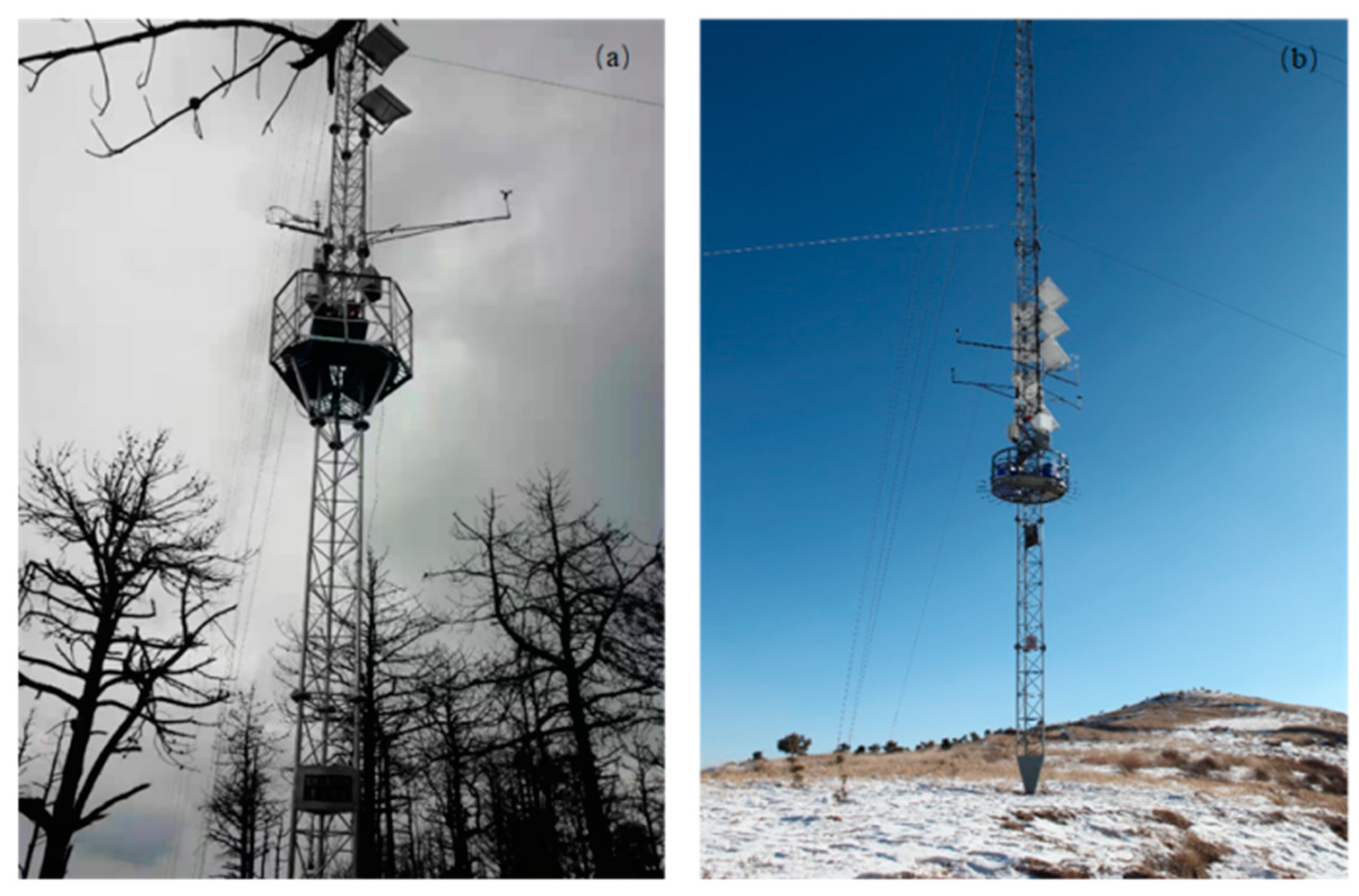
Site 1, located in the alpine mixed forests of the western Sichuan Plateau, is surrounded by relatively steep hillsides (102.087° E, 27.628° N, 2786 m above sea level). The underlying surface is mainly covered by shrubs, weeds, and pines about 5 m tall (Figure 1a). Site 2 is located on a gentle slope near the ridge (111.991° E, 39.272° N, 1800 m above sea level, 500 m above the foothill village). The local terrain is relatively flat, which is a typical Loess Plateau landform. The underlying surface is covered by sparse trees and weeds usually less than 30 cm (Figure 1b). 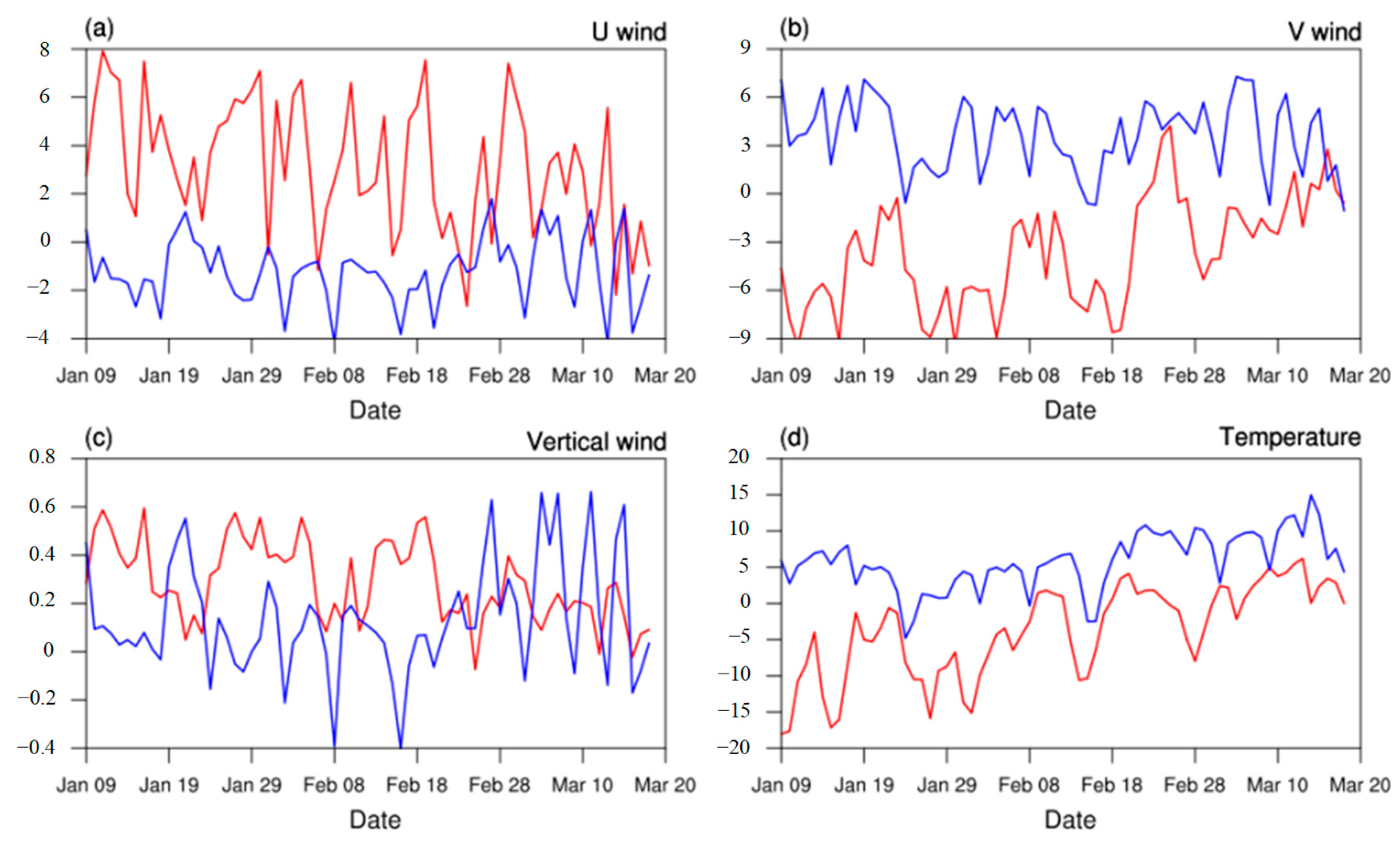Figure 2 shows the eddy covariance data at the two sites.

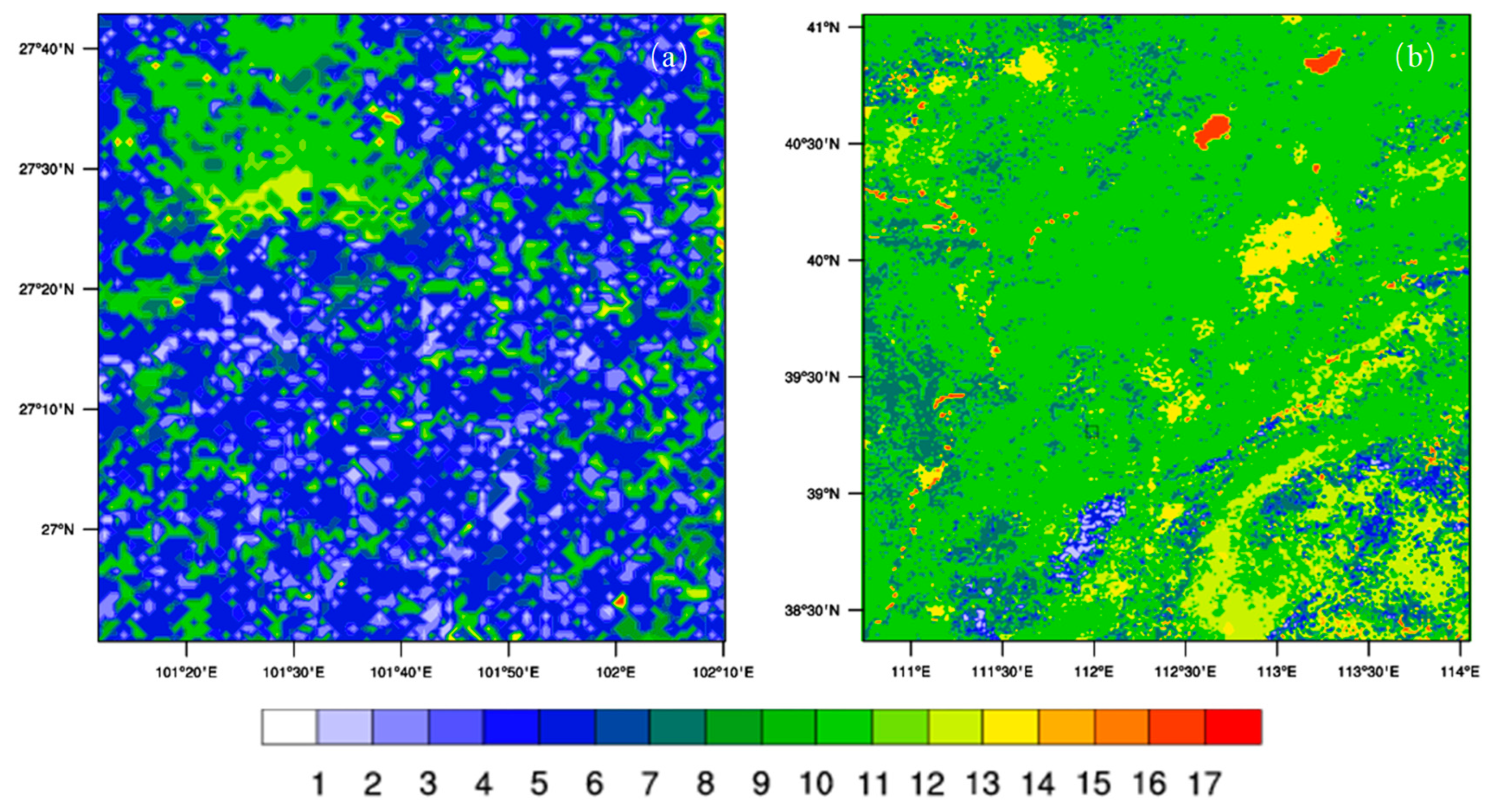
The local land use categories of the Weather Research and Forecasting (WRF) Model near the two sites are shown in Figure 3. The land use categories are shown in

Table 1. Land use categories.

Land Use Category	Land Use Description	Land Use Category	Land Use Description
1	Evergreen needleleaf forest	10	Grasslands
2	Evergreen broadleaf forest	11	Permanent wetlands
3	Deciduous needleleaf forest	12	Croplands
4	Deciduous broadleaf forest	13	Urban and built-up
5	Mixed forests	14	Cropland/natural vegetation mosaic
6	Closed shrubland	15	Snow and ice
7	Open shrublands	16	Barren or sparsely vegetated
8	Woody savannas	17	Water
9	Savannas

. The land use description of the mixed forest near site 1 is completely different from the land use description of the grassland near site 2.

The data of the two sites are measured by the eddy covariance system at 10 m above the ground, consisting of a three-axis Sonic Anemometer (CSAT3B, Campbell Scientific Inc., Logan, UT, US) with the sampling frequency of 10 Hz. The data files with a 0.1 s time resolution contain three wind components for the $x$, $y$, and $z$ directions, air temperature, CO₂ concentration, water vapor concentration, and air pressure.

The observation period at site 1 is from 9 January to 20 March 2020, while the observation period at site 2 is from 9 January to 20 March 2021.

3. Data and Method

3.1. Data Processing

To eliminate the systematic errors caused by instrument failure, maintenance, weather, power supply, etc., the original data is managed by following quality control procedures [25]:

(1)

The horizontal wind speed out of ±30 m.s⁻¹ and the vertical wind speed out of ±10 m.s⁻¹ are removed, same as the temperature out of ±50 °C, and the abnormal characteristics of the general climatic statistical are excluded.

(2)

Data with a variance greater than 5 times are eliminated.

(3)

Random errors of the data receiving and transmission system caused by non-human factors, such as condensation on the sensor, are eliminated. Values of $\left|X_{i+2}-X_i\right|>5\sigma$ are considered as random pulses for removal, where $X$ is the time series and $\sigma$ is the variance.

(4)

The static wind data with wind speed less than 1 m.s⁻¹ is removed.

To facilitate the calculation, the coordinates of the data are rotated twice every 30 min [26,27]. Firstly, the $x$-$y$ plane is rotated around the $z$-axis to make the $x$-$z$ plane consistent with the mean wind direction and $\overline{v_1}=0$. The measured wind component is denoted by the subscript m and the wind component after the first rotation is denoted by the subscript 1. The wind components after the first rotation are calculated as:

$$\begin{gathered} u_1=u_m\cos \alpha +v_m\sin \alpha \\ {v}_1=-u_m\sin \alpha +v_m\cos \alpha \\ {w}_1=w_m \end{gathered}$$

(1)

where the rotation angle is calculated as:

$$\alpha ={\tan }^{-1}\left(\overline{v_m}/\overline{u_m}\right)$$

(2)

The coordinate is rotated for a second time to eliminate the error caused by an uneven installation of the instrument, and the wind component is denoted by the subscript 2. The $x$-$z$ plane is rotated around the $y$-axis to make $\overline{w_2}=0$. The wind components after the second rotation are calculated as:

$$\begin{gathered} u_2=u_1\cos \beta +w_1\sin \beta \\ {v}_2=v_1 \\ {w}_2=-u_1\sin \beta +w_1\cos \beta \end{gathered}$$

(3)

where the rotation angle is calculated as:

$$\beta ={\tan }^{-1}\left(\overline{w_1}/\overline{u_1}\right)$$

(4)

After the second rotation, the mean wind speed, $\overline{u}=U_{mean}=\sqrt{{\overline{u}}^2+{\overline{v}}^2+{\overline{w}}^2}$, is along the mean streamline.

3.2. Obukhov Length

According to the Monin–Obukhov similarity theory in the surface layer, the Obukhov length is calculated as [28,29,30]:

$$L=-\frac{u_{*}^3}{\kappa \frac{g}{T_0}\overline{w^{\prime }{T}_0^{\prime }}}$$

(5)

where $u_{*}={\left({\overline{u^{\prime }{w}^{\prime }}}^2+{\overline{v^{\prime }{w}^{\prime }}}^2\right)}^{\frac{1}{4}}$ is the friction velocity; $\kappa =0.4$ is the von Karman constant; $g=9.8 m·s^{-2}$ is the acceleration of gravity; $T_0$ is the mean temperature in 30 min; $u^{\prime }$, $v^{\prime }$, and $w^{\prime }$ are three wind component fluctuations of the $x$, $y$, and $z$ directions, respectively; and $T_0^{\prime }$ is the temperature fluctuation.

3.3. Eddy Covariance Technique

In a certain average time (30 min), the turbulent flux of a certain scalar, $x$ (set mass density [kg.m⁻³] as the unit), can be expressed by the following equation:

$$F_x=\overline{w·x}[\mathrm{kg}.{\mathrm{m}}^{-2}.{\mathrm{s}}^{-1}]$$

(6)

where the horizontal line above represents the time average. The measured quantity is divided into two parts: the average quantity and the pulsation quantity:

$$w=\overline{w}+w^{\prime }$$

(7)

$$x=\overline{x}+x^{\prime }$$

(8)

then Equation (6) becomes:

$$Q_x=\overline{w}·\overline{x}+\overline{w^{\prime }{x}^{\prime }}=\overline{w^{\prime }{x}^{\prime }}$$

(9)

where the time-averaged vertical wind speed is assumed to be zero ($\overline{w}=0$). Subsequently, the calculation equations of momentum flux ($\tau$), sensible heat flux ($H_s$), and latent heat flux ($H_L$) are [31,32]:

$$\tau =-\rho u_{*}^2[\mathrm{N}.{\mathrm{m}}^{-2}]$$

(10)

$$H_s=\rho C_p\overline{w^{\prime }{T}^{\prime }}[\mathrm{W}.{\mathrm{m}}^{-2}]$$

(11)

$$H_L=\lambda \overline{w^{\prime }{\rho }_v^{\prime }}[\mathrm{W}.{\mathrm{m}}^{-2}]$$

(12)

where $\rho$ is the air density; $C_p$ is the constant pressure specific heat; $\mathsf{\lambda }$ is the latent heat of evaporation; and ${\rho }_v$ is the observed water vapor density [33,34]. All basic and calculated variables have been analyzed in

Table 2. Variables.

Category	Basic Variables	Category	Calculated Variables
1	U wind	1	Friction velocity ($u_{*}$)
2	V wind	2	Heat flux
3	Vertical wind	3	Obukhov length ($L$)
4	Air temperature	4	Density ($\rho$)
5	Mixed forests	5	Momentum flux ($\tau$)
6	CO2 concentration	6	Specific humidity
7	Water vapor concentration	7	Constant pressure specific heat ($C_p)$
8	Air pressure	8	Latent heat of evaporation ($\mathsf{\lambda })$
		9	Sensible(latent) heat flux ($H_L/H_s$)

.

4. Results and Discussion

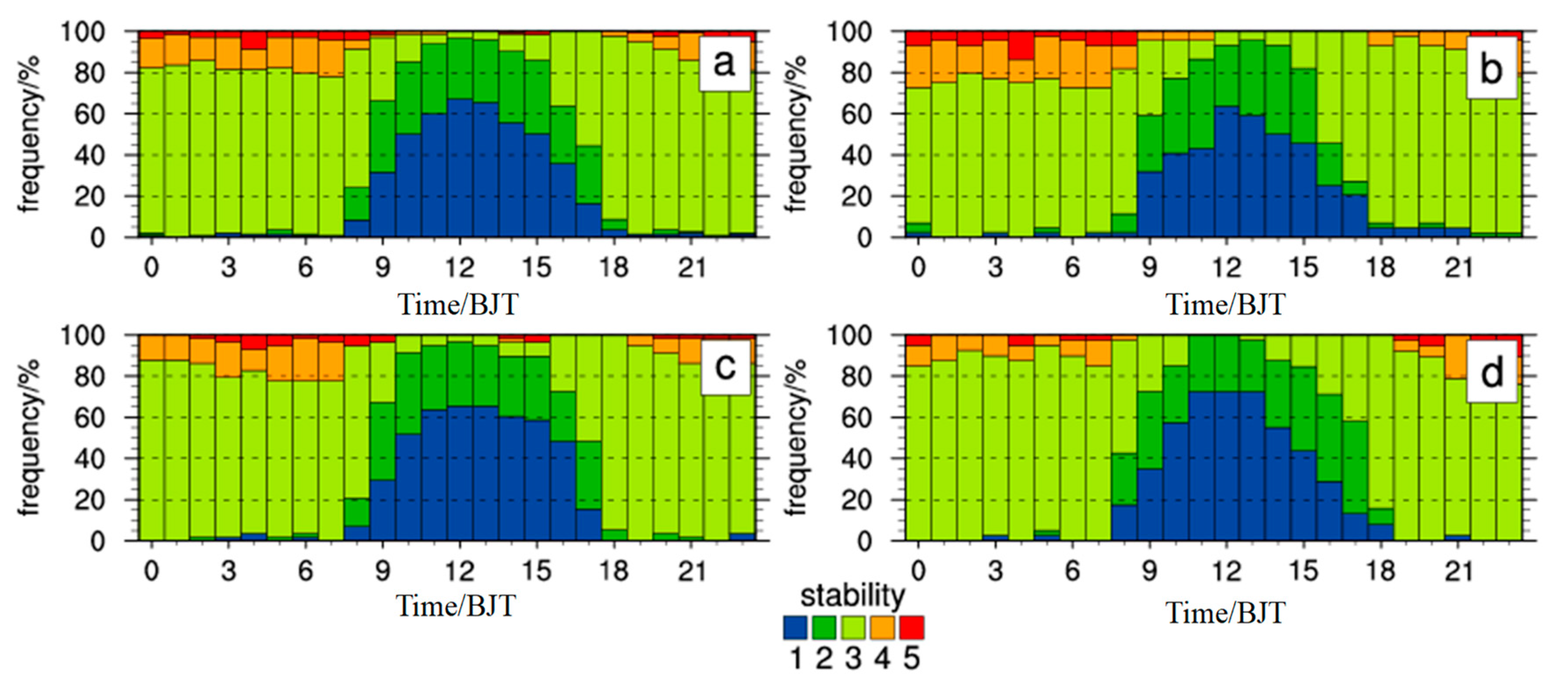
To study the diurnal variation characteristics of atmospheric stability on the complex terrain of the Yalong River Basin, $L$ is calculated as shown in Equation (5) based on the observed data from site 1 (Figure 4). The atmospheric stability categories are shown in

Table 3. Categories of $L$ and atmospheric stability.

$\mathbf{The}\mathbf{Range}\mathbf{of}\mathit{L}$	The Atmospheric Stability	Categories
−150 ≤ $L$ < 0	Unstable	1
−500 ≤ $L$ < −150	Weak-unstable	2
$L$ > 500 or $L$ < −500	Neutral	3
100 < $L$ ≤ 500	Weak-stable	4
0 < $L$ ≤ 100	Stable	5

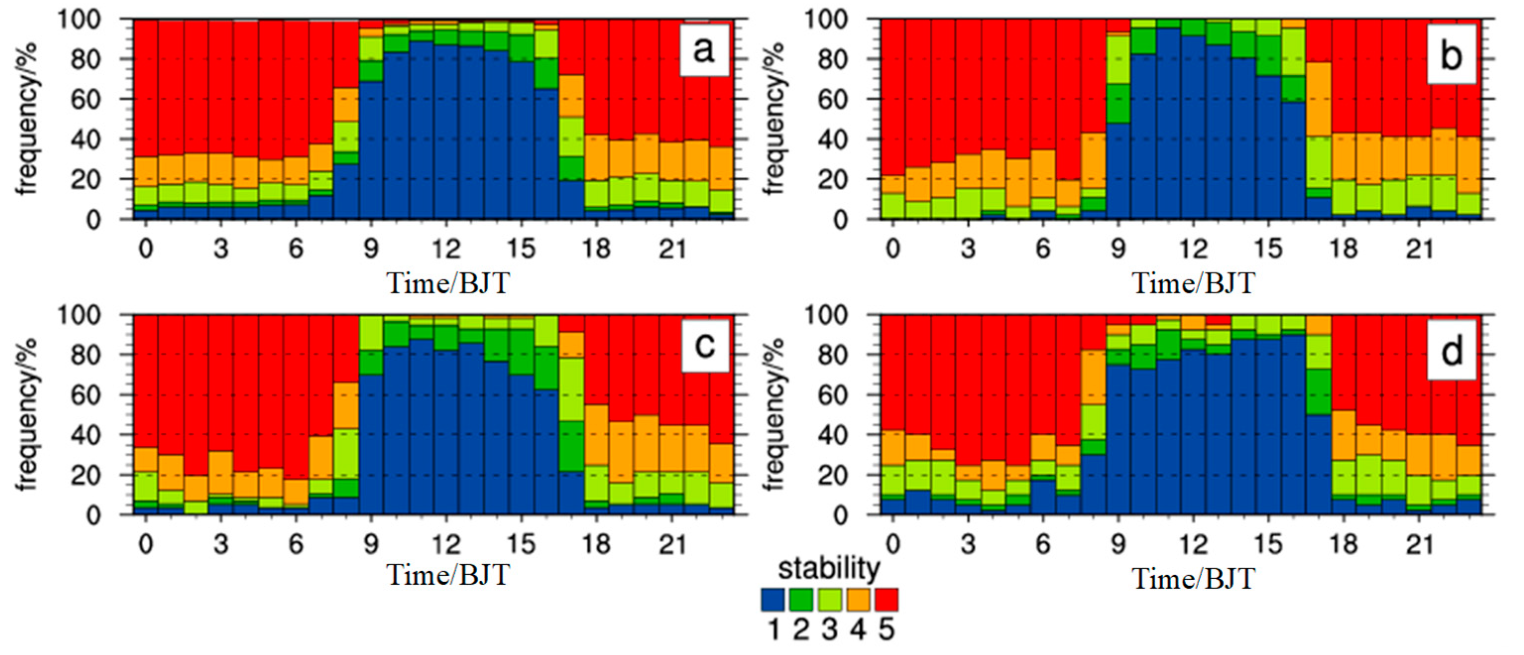
. As shown in Figure 4, the relative proportion of the neutral and the unstable boundary layer changes significantly at 8:00 (Beijing Time, BJT, the same as below) and 18:00. The dominant boundary layer transforms from the neutral boundary layer to the unstable boundary layer at 8:00, and it is the opposite at 18:00. From 18:00 to 8:00 the next day, the boundary layer is dominated by a neutral boundary layer with a certain proportion of a weak-stable and stable boundary layer. From 8:00 to 18:00, the boundary layer is dominated by a weak-unstable and unstable boundary layer. The proportion of the unstable boundary layer is more than 90% and reaches a peak of the day at 12:00.

With the same method as site 1, the diurnal variation characteristics of atmospheric stability on the complex terrain of the Loess Plateau is plotted (Figure 5). It can be seen that the relative proportion of the stable and unstable boundary layer changes significantly at 7:00 and 18:00. The dominant boundary layer transforms from the stable boundary layer to the unstable boundary layer at 7:00 (1 h earlier than that at site 1), and it is the opposite at 18:00. From 18:00 to 7:00 the next day, the boundary layer is dominated by the stable boundary layer, with a certain proportion of the weak-stable boundary layer. From 7:00 to 18:00, the unstable boundary layer is dominated with a certain proportion of the weak-unstable boundary layer. Comparing the changes of the atmospheric boundary layer at the two sites, it can be derived that the nighttime dominant boundary layer at site 1 is the neutral boundary layer, while at site 2 it is the stable boundary layer.

Correspondingly, the distribution of atmospheric stability in different periods at site 1 is analyzed in

Table 4. The distribution of atmospheric stability at site 1.

Categories	1	2	3	4	5
0109–0320	19.08%	13.28%	58.23%	7.36%	2.06%
0109–0131	16.95%	12.62%	58.10%	9.60%	2.73%
0201–0229	19.83%	13.15%	58.33%	6.90%	1.80%
0301–0320	20.36%	14.21%	58.22%	5.51%	1.70%

. During the study period, the surface layer is dominated by the neutral boundary layer, with a proportion of more than 50%, followed by the unstable boundary layer, accounting for more than 30%. The occurrence probability of the stable boundary layer is the lowest, only about 10%. At site 2, the stable boundary layer is the main, accounting for nearly 40%, followed by the unstable boundary layer, accounting for about 30%. The proportion of the weak-unstable boundary layer is the lowest, less than 6% (

Table 5. The distribution of atmospheric stability at site 2.

Categories	1	2	3	4	5
0109–0320	30.37%	5.84%	10.92%	13.12%	39.76%
0109–0131	27.45%	4.89%	11.14%	14.86%	41.67%
0201–0229	29.61%	7.14%	10.27%	13.47%	39.51%
0301–0320	34.79%	5.10%	11.56%	10.63%	37.92%

). Compared with previous results, the diurnal variation characteristics and the distribution of atmospheric stability at the two sites are quite different from those in Xilinhot, Jiangxi, and the Netherlands [25]. This may be caused by the differences in the topography and the underlying surface between the two sites. Site 1 is located in the hinterland of the western Sichuan Plateau and on the east bank of the Yalong River. It is a complex mountainous terrain of the plateau and the underlying surface is mixed forest. The topographic effect has an impact on the anemometer tower, thus, the neutral boundary layer dominated during the nighttime at site 1. Site 2 is located on the Loess Plateau. Although the overall altitude is high, the local underlying surface is a flat and gentle slope, thus the diurnal variation characteristics of the atmospheric stability at site 2 is essentially consistent with the classical similarity theory.

Accordingly, the average horizontal wind speed at 10 m above the ground at different atmospheric stabilities during each period at the two sites can be calculated (Table 5 and

Table 6. The average horizontal wind speed at 10 m above the ground at different atmospheric stabilities at site 1.

Categories	1	2	3	4	5
0109–0320	2.57 ± 1.72 m/s	4.59 ± 2.54 m/s	6.12 ± 3.17 m/s	3.67 ± 1.89 m/s	3.35 ± 1.98 m/s
0109–0131	2.30 ± 1.48 m/s	4.48 ± 2.71 m/s	6.16 ± 3.22 m/s	3.23 ± 1.78 m/s	2.83 ± 1.93 m/s
0201–0229	2.60 ± 1.79 m/s	4.42 ± 2.38 m/s	5.91 ± 3.28 m/s	4.00 ± 2.08 m/s	3.87 ± 1.85 m/s
0301–0320	2.79 ± 1.84 m/s	4.94 ± 2.58 m/s	6.38 ± 2.96 m/s	3.92 ± 1.77 m/s	3.50 ± 2.27 m/s

). Compared with site 2, the horizontal wind speed at site 1 is significantly smaller at the same atmospheric stability. As evident from Table 6, the horizontal wind speed in the neutral (unstable) boundary layer is significantly higher (lower) than that at the other atmospheric stability at site 1. As shown in

Table 7. The average horizontal wind speed at 10 m above the ground at different atmospheric stabilities at site 2.

Categories	1	2	3	4	5
0109–0320	6.02 ± 3.41 m/s	8.30 ± 4.65 m/s	8.04 ± 4.57 m/s	7.89 ± 3.32 m/s	5.40 ± 2.52 m/s
0109–0131	6.95 ± 3.44 m/s	11.31 ± 4.15 m/s	9.74 ± 3.44 m/s	9.77 ± 2.73 m/s	5.86 ± 2.56 m/s
0201–0229	6.43 ± 3.75 m/s	8.15 ± 4.12 m/s	7.42 ± 4.34 m/s	7.51 ± 3.06 m/s	5.40 ± 2.66 m/s
0301–0320	4.77 ± 2.49 m/s	3.99 ± 2.37 m/s	6.53 ± 5.47 m/s	5.42 ± 2.84 m/s	4.86 ± 2.13 m/s

, the horizontal wind speed in the neutral and weak-unstable boundary layers are clearly higher than that in other boundary layers, and in the stable boundary layer it is the smallest. This result is consistent with the opinion of Gong et al. [25], and it is because wind shear is the main source of turbulent energy in the neutral boundary layer and buoyancy is negligible. While in the non-neutral boundary layer, the dynamic and thermodynamic factors act simultaneously. However, the difference of the stability variations and the average horizontal wind speed at 10 m above the ground of the two sites are likely associated with the discrepancy of the momentum and heat flux transfer caused by the diverse underlying surfaces. Therefore, the variations of the momentum and heat flux at the two sites are investigated.

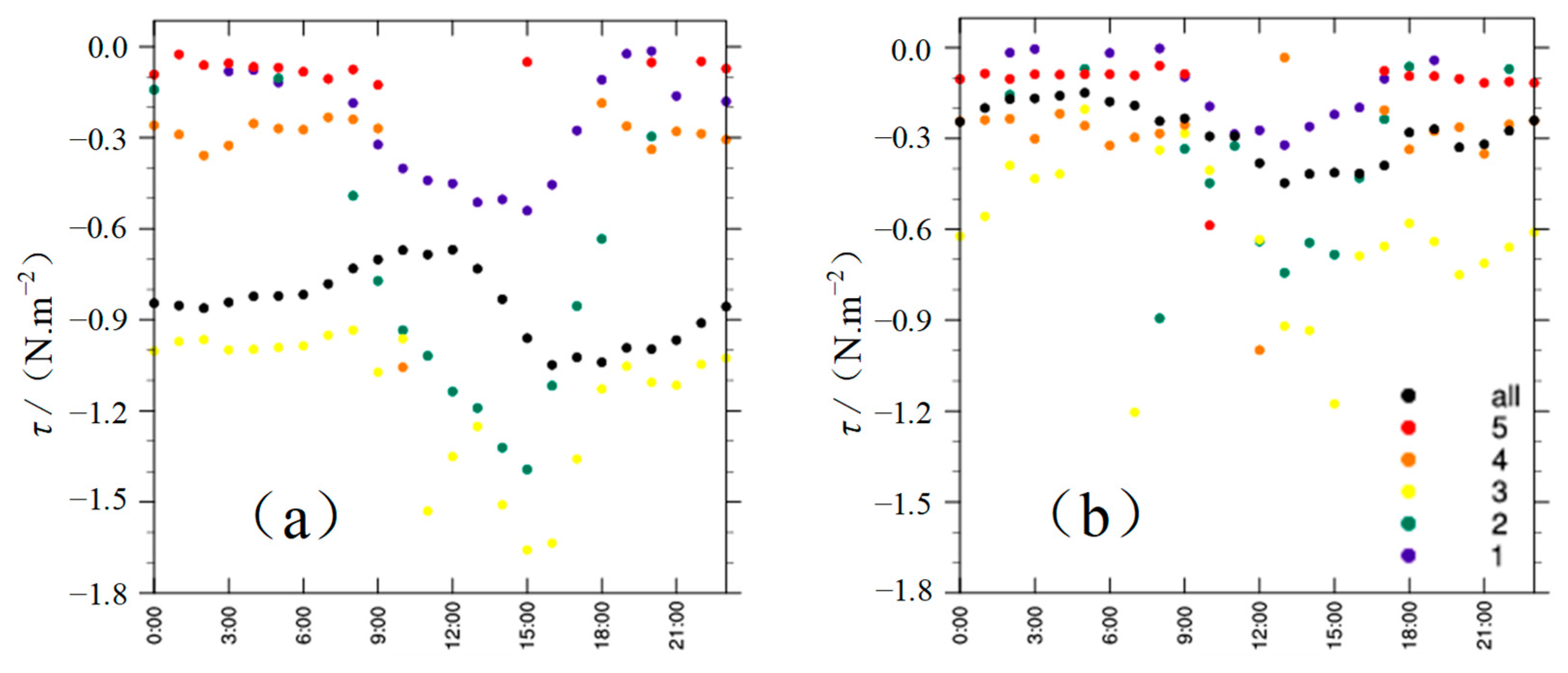
The greater the absolute value of the momentum flux is, the greater the kinetic energy in the surface layer is, and the stronger the vertical upward transport of the turbulence is. Figure 6 shows the variation of the momentum flux at the two sites. On the whole, the diurnal variations of the momentum flux at the two sites are all unimodal. In different boundary layers, the momentum flux is the largest in the neutral, followed by in the weak-unstable, and the smallest in the stable, which is in accordance with the conclusion obtained above. Compared with site 2, the average momentum flux at site 1 is evidently larger, and the diurnal range of the momentum flux at site 1 (0.379 N.m⁻²) is greater than that at site 2 (0.297 N.m⁻²). Compared with the values of Yuzhong in Gansu (0.08 N.m⁻²) and Tongyu in Jilin (0.25 N.m⁻²) [21], the diurnal range of the momentum flux at site 1 is clearly higher, which may be mainly caused by the complex underlying surface (alpine mixed forests of the western Sichuan Plateau), and at site 2 it is similar with that in Tongyu.

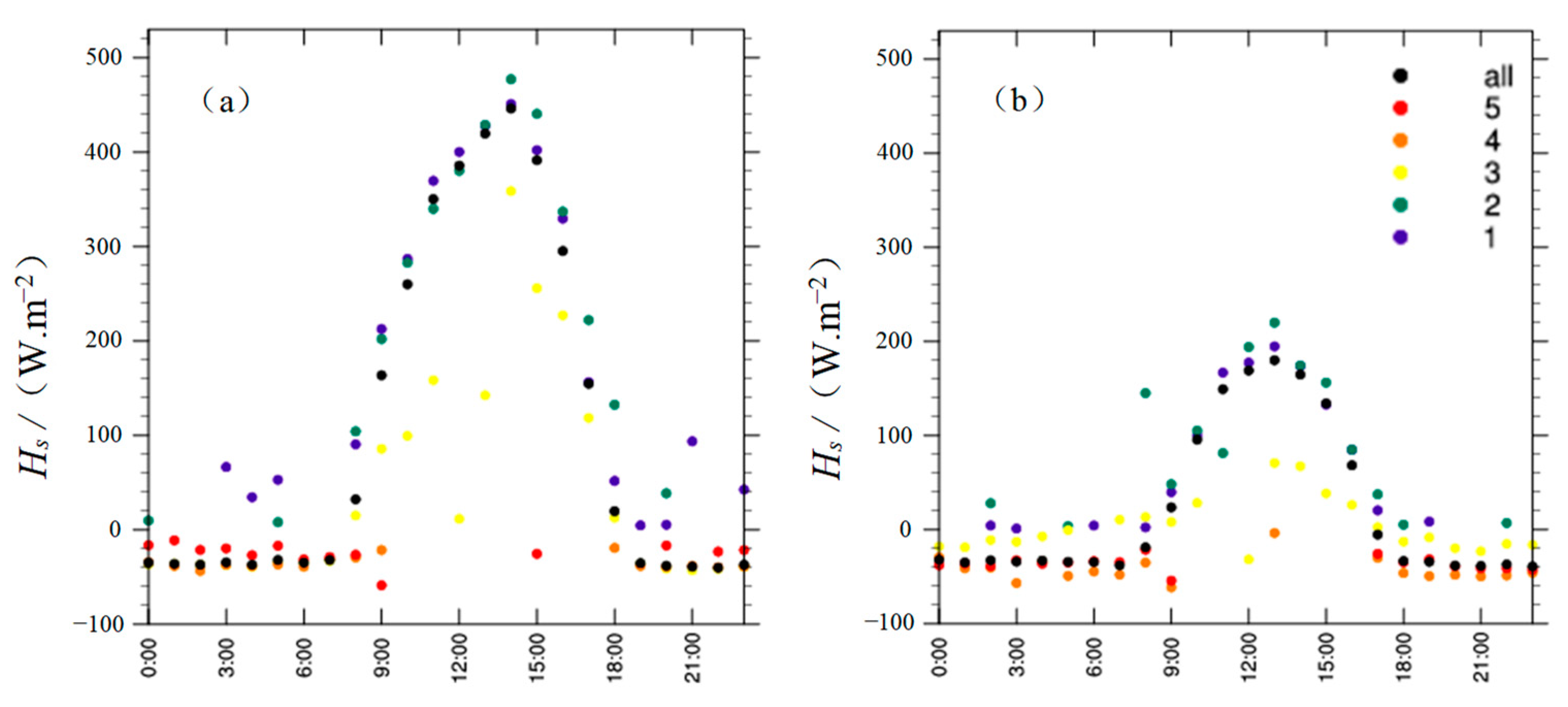
Figure 7 shows the diurnal variation of the sensible heat flux at the two sites. The diurnal variations of the sensible heat flux at the two sites are all unimodal and values of the sensible heat flux change remarkably at 8:00 and 18:00. Due to enhanced solar radiation at 8:00, a sharp vertical temperature gradient is generated in the surface layer to promote the development of turbulence. At this time, the sensible heat flux begins to change from the negative to the positive, implying that the ground cooling effect during the nighttime converts to the ground heating effect. After that, the sensible heat flux continues to increase and reaches a peak value between 13:00 and 15:00. Hereafter, the sensible heat flux gradually decreases. Between 18:00 and 19:00, the sensible heat flux turns to negative again. It means that the sun sets at this time and the solar radiation received by the surface layer is weakened, thus the vertical temperature gradient is reduced and the energy provided by thermal driving for the development of turbulence is reduced. From 19:00 to 7:00 the next day, the sensible heat flux remains near zero. In the different stability, values of the sensible heat flux are in the order: the weak-unstable boundary layer > the unstable boundary layer > the neutral boundary layer > the stable boundary layer > the weak-stable boundary layer, illustrating the dominant role of thermal driving in the unstable boundary layer. Compared with site 2, the peak time at site 1 (14:00) is 1 h behind site 2 (13:00). The peak value of site 1 (446.239 W.m⁻²) is two and a half times as much as that of site 2 (180.035 W.m⁻²), and both are higher than those of Yuzhong, Gansu (140.3 W.m⁻²) and Jilin Tongyu (157.3 W.m⁻²) [21]. It is mainly because the altitude of site 1 is higher than that of site 2, there is a difference in solar radiation intensity, resulting in a large discrepancy in the sensible heat flux between the two sites.

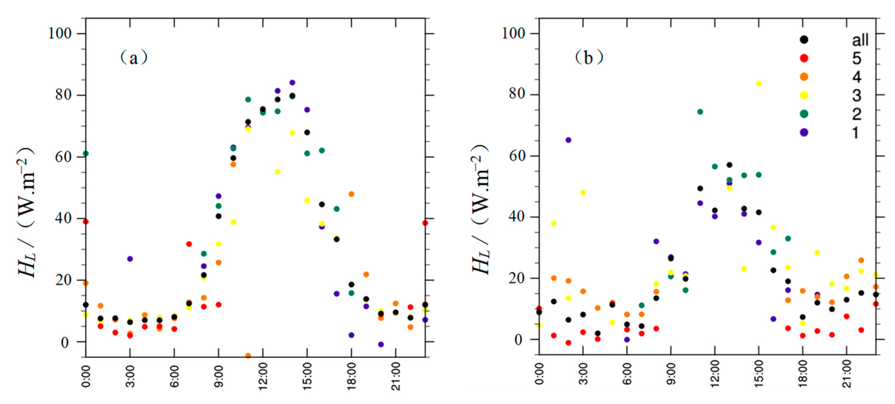
Figure 8 shows the diurnal variation of the latent heat flux in the surface layer at the two sites. The diurnal variations of the latent heat flux at the two sites are all unimodal. In a different stability, the latent heat flux in the unstable and weak-unstable boundary layers are the largest, followed by the neutral boundary layer, and in the stable and weak-stable boundary layers are the smallest, maintaining below 10 W.m⁻². Comparing the diurnal variation of the latent heat flux at the two sites, it can be seen that the peak value at site 1 (79.902 W.m⁻²) appears at 14:00, while the peak value at site 2 (57.082 W.m⁻²) appears at 13:00. Compared with those values of Gansu Yuzhong in the summer (195.4 W.m⁻²) and Jilin Tongyu in the summer (211.4 W.m⁻²) [21], the peak values of the latent heat flux at the two sites are significantly low. This is because our study periods of the two sites are relatively dry, resulting in a lower latent heat flux than Yuzhong and Tongyu.

5. Conclusions

The diurnal variations of atmospheric stability and fluxes are analyzed by studying the local eddy covariance data from two typical topographies: the complex mountainous area along the Yalong River Basin (in western China, site 1) and the relatively flat Nanhua Mountain in Shanxi (in central China, site 2), which partly reflects the difference in the energy exchange process between different underlying surfaces and the atmospheric boundary layer.

The conclusions are as follows:

(1)

The dominant boundary layer at site 1 during nighttime is the neutral boundary layer, while at site 2 it is the stable.

(2)

The average wind speed at 10 m above the ground of site 1 is significantly lower than that of site 2. At site 1, the wind speed is the highest in the neutral boundary layer and it is the smallest in the unstable boundary layer. Contrastingly, at site 2 the wind speed is the highest in the neutral and weak-unstable boundary layers, and it is the smallest in the stable boundary layer.

(3)

The diurnal variations of the momentum flux at the two sites are both unimodal, but the peak time is distinct. The daily range of the momentum flux at site 1 is significantly higher than that at site 2.

(4)

The diurnal variation of the sensible heat flux is unimodal. The peak value of site 1 (446.239 W.m⁻²) is two and a half times as much as that of site 2 (180.035 W.m⁻²), and both are higher than those of Yuzhong, Gansu (140.3 W.m⁻²) and Jilin Tongyu (157.3 W.m⁻²) [21]. The peak time at site 1 (14:00) is 1 h behind site 2 (13:00).

(5)

The diurnal variation of the latent heat flux is unimodal. The peak value at site 1 is slightly higher than that at site 2, and the peak time at site 1 lags behind site 2 by 1 h. Compared with those values of Gansu Yuzhong in the summer (195.4 W.m⁻²) and Jilin Tongyu in the summer (211.4 W.m⁻²) [21], the peak values at the two sites are significantly low.

References

1. Pan, B.T.; Han, J.F.; Li, B.Y. Basic terrestrial geomorphological types in China and their circumscriptions. Quat. Sci. 2008, 28, 535–543. (In Chinese) [Google Scholar]
2. Liu, Z.Y.; Li, Y.Y.; He, Y. A preliminary study on the main causes of negative shear in ultra-high altitude area. Adhesion 2019, 40, 56–62. (In Chinese) [Google Scholar]
3. Gualtieri, G.; Secci, S. Comparing methods to calculate atmospheric stability-dependent wind speed profiles: A case study on coastal location. Renew. Energy 2011, 36, 2189–2204. [Google Scholar] [CrossRef]
4. Hansen, K.S.; Barthelmie, R.J.; Jensen, L.E.; Sommer, A. The impact of turbulence intensity and atmospheric stability on power deficits due to wind turbine wakes at Horns Rev wind farm. Wind Energy 2012, 15, 183–196. [Google Scholar] [CrossRef] [Green Version]
5. Han, X.X.; Liu, D.Y.; Xu, C.; Shen, W.Z. Atmospheric stability and topography effects on wind turbine performance and wake properties in complex terrain. Renew. Energy 2018, 126, 640–651. [Google Scholar] [CrossRef]
6. Bardal, L.M.; Onstad, A.E.; Sætran, L.R.; Lund, J.A. Evaluation of methods for estimating atmospheric stability at two coastal sites. Wind Eng. 2018, 42, 561–575. [Google Scholar] [CrossRef]
7. Pérez Albornoz, C.; Escalante Soberanis, M.A.; Ramírez Rivera, V.; Rivero, M. Review of atmospheric stability estimations for wind power applications. Renew. Sustain. Energy Rev. 2022, 163, 112505. [Google Scholar] [CrossRef]
8. Jin, L.L. Research of Boundary Layer Characteristics in Urumqi; Nanjing University of Information Science and Technology: Nanjing, China, 2015. (In Chinese) [Google Scholar]
9. Sathe, A.; Gryning, S.; Peña, A. Comparison of the atmospheric stability and wind profiles at two wind farm sites over a long marine fetch in the North Sea. Wind Energy 2011, 14, 767–780. [Google Scholar] [CrossRef]
10. Sathe, A.; Mann, J.; Barlas, T.; Bierbooms, W.A.A.M.; van Bussel, G.J.W. Influence of atmospheric stability on wind turbine loads. Wind Energy 2012, 16, 1013–1032. [Google Scholar] [CrossRef]
11. Gryning, S.E.; Batchvarova, E.; Brümmer, B.; Jørgensen, H.; Larsen, S. On the extension of the wind profile over homogeneous terrain beyond the surface boundary layer. Bound-Layer Meteorol. 2007, 124, 251–268. [Google Scholar] [CrossRef]
12. Sathe, A.; Bierbooms, W. Influence of different wind profiles due to varying atmospheric stability on the fatigue life of wind turbines. J. Phys. Conf. Ser. 2007, 75, 012056. [Google Scholar] [CrossRef] [Green Version]
13. Jammet, M.; Dengel, S.; Kettner, E.; Parmentier, F.J.W.; Wik, M.; Crill, P.; Friborg, T. Year-round CH4 and CO2 flux dynamics in two contrasting freshwater ecosystems of the subarctic. Biogeosci. Discuss. 2017, 14, 5189–5216. [Google Scholar] [CrossRef]
14. Erkkilä, K.M.; Ojala, A.; Bastviken, D.; Biarmann, T.; Heiskanen, J.J.; Lindroth, A.; Peltola, O.; Rantakari, M.; Vesala, T.; Mammarella, I. Methane and carbon dioxide fluxes over a lake: Comparison between eddy covariance, floating chambers and boundary layer method. Biogeoences 2018, 15, 429–445. [Google Scholar] [CrossRef] [Green Version]
15. Clement, R.J.; Moncrieff, J.B. A functional approach to vertical turbulent transport of scalars in the atmospheric surface layer. Bound. Layer Meteorol. 2019, 173, 373–408. [Google Scholar] [CrossRef] [Green Version]
16. Barskov, K.; Stepanenko, V.; Repina, I.; Artamonov, A.; Gavrikov, A. Two regimes of turbulent fluxes above a frozen small lake surrounded by forest. Bound. Layer Meteorol. 2019, 173, 311–320. [Google Scholar] [CrossRef]
17. Esters, L.; Rutgersson, A.; Nilsson, E.; Sahlée, E. Non-local impacts on eddy-covariance air-lake CO2 fluxes. Bound. Layer Meteorol. 2021, 178, 283–300. [Google Scholar] [CrossRef]
18. Sigmund, A.; Dujardin, J.; Comola, F.; Sharma, V.; Huwald, H.; Melo, D.B.; Hirasawa, N.; Nishimura, K.; Lehning, M. Evidence of strong flux underestimation by bulk parametrizations during drifting and blowing snow. Bound. Layer Meteorol. 2021, 182, 119–146. [Google Scholar] [CrossRef]
19. Liu, C.X.; Wan, Q.L.; Liao, F.; Zhao, Z.K. Surface observations in the tropical cyclone environment over the South China Sea. J. Trop. Meteorol. 2012, 18, 263–274. [Google Scholar]
20. Duan, Z.Q.; Yao, X.H.; Li, Y.P.; Lei, X.T.; Fang, P.Z.; Zhao, B.K. Investigation of turbulent momentum flux in the typhoon boundary layer. J. Geophys. Res. Oceans 2017, 122, 2259–2268. [Google Scholar] [CrossRef]
21. Chen, L.J.; Zhang, L.; Liang, J.N.; Zhou, X. Analysis of turbulent flux on different underlying surfaces over Semi-arid area. Plateau Meteorol. 2017, 36, 1325–1335. (In Chinese) [Google Scholar]
22. He, Y.Y.; Hu, F.; Liu, Y.J.; Liu, L. Boundary layer characteristics during a heavy PM2.5 pollution process in Beijing. Clim. Environ. Res. 2019, 24, 61–72. (In Chinese) [Google Scholar]
23. Wang, G.Y.; Huang, J.P.; Guo, W.D.; Zuo, J.Q.; Wang, J.M.; Bi, J.R.; Huang, Z.W.; Shi, J.S. Observation analysis of land-atmosphere interactions over the Loess Plateau of northwest China. J. Geophys. Res. Atmos. 2010, 115, D00K17. [Google Scholar] [CrossRef] [Green Version]
24. Sun, J.; Hu, W.F.; Wang, N.A.; Zhao, L.Q.; An, R.; Ning, K.; Zhang, X.H. Eddy covariance measurements of water vapor and energy flux over a lake in the Badain Jaran Desert, China. J. Arid Land 2018, 10, 517–533. [Google Scholar] [CrossRef] [Green Version]
25. Gong, X.; Zhu, R.; Li, Z.C. Study of near-surface wind shear exponents of different regions in China. Meteorol. Mon. 2018, 44, 1160–1168. (In Chinese) [Google Scholar]
26. Li, Z.J.; He, Q.; Jin, L.L.; Ali, M.M.T.M.; Zhao, J.W. Comparative analysis of different coordinate rotation methods for eddy fluxes in Tazhong station. Desert Oasis Meteorol. 2019, 13, 105–111. (In Chinese) [Google Scholar]
27. Liu, L.; Wang, T.J.; Sun, Z.H.; Wang, Q.G.; Zhuang, B.L.; Han, Y.; Li, S. Eddy covariance tilt corrections over a coastal mountain area in South-East China: Significance for near-surface turbulence characteristics. Adv. Atmos. Sci. 2012, 29, 1264–1278. [Google Scholar] [CrossRef]
28. Monin, A.S.; Obukhov, A.M. Basic laws of turbulent mixing in the ground layer of the atmosphere. Contrib. Geophys. Inst. Acad. Sci. USSR 1954, 24, 163–187. [Google Scholar]
29. Gong, X.; Zhu, R.; Li, Z.C. A study of near surface wind profiles in the Hebei coastal area based on observational experiments. J. Trop. Meteorol. 2018, 24, 508–514. [Google Scholar]
30. Lyu, R.; Hu, F.; Liu, L.; Xu, J.J.; Cheng, X.L. High-order statistics of temperature fluctuations in an unstable atmospheric surface layer over grassland. Adv. Atmos. Sci. 2018, 35, 1265–1276. [Google Scholar] [CrossRef]
31. Zuo, J.Q.; Huang, J.P.; Wang, J.M.; Zhang, W.; Bi, J.R.; Wang, G.Y.; Li, W.J.; Fu, P.J. Surface turbulent flux measurements over the Loess Plateau for a semi-arid climate change study. Adv. Atmos. Sci. 2009, 26, 679–691. [Google Scholar] [CrossRef]
32. Bi, X.Y.; Wen, B.; Zhao, Z.K.; Huang, J.; Liu, C.X.; Huang, H.J.; Mao, W.K.; Wen, G.H. Evaluation of corrections on turbulent fluxes obtained by eddy covariance method in high winds. J. Trop. Meteorol. 2018, 24, 176–184. [Google Scholar]
33. Wang, J.M.; Wang, W.Z.; Ao, H.Y.; Sun, F.L.; Wang, S.G. Turbulence flux measurements under complicated conditions. Adv. Earth Sci. 2007, 22, 791–797. (In Chinese) [Google Scholar]
34. Wang, J.M. Eddy Covariance Flux Observation Guidebook (Ver. 20120212). 2012. Available online: http://westdc.westgis.ac.cn/water/surveystd (accessed on 22 November 2021). (In Chinese).
Figure 1. Eddy covariance observation system at (a) site 1 and (b) site 2.
Atmosphere 13 02108 g001
Figure 2. Eddy covariance observation data. (a) U wind (unit: m s−1), (b) V wind (unit: unit: m s−1), (c) vertical wind (unit: m s−1), and (d) temperature (°C). Blue line is observed at site 1. The red line is observed at site 2.
Atmosphere 13 02108 g002
Figure 3. Land use categories at (a) site 1 and (b) site 2.
Atmosphere 13 02108 g003
Figure 4. The diurnal variation of atmospheric stability at site 1. (a) 9 January–20 March 2020; (b) January; (c) February; and (d) March. Stability level 1: unstable; 2: weak-unstable; 3: neutral; 4: weak-stable; and 5: stable.
Atmosphere 13 02108 g004
Figure 5. The diurnal variation of atmospheric stability at site 2. (a) 9 January–20 March 2021; (b) January; (c) February; and (d) March.
Atmosphere 13 02108 g005
Figure 6. The diurnal variation of the momentum flux in different atmospheric stability at (a) site 1 and (b) site 2. Stability level 1: unstable; 2: weak-unstable; 3: neutral; 4: weak-stable; and 5: stable.
Atmosphere 13 02108 g006
Figure 7. The diurnal variation of the sensible heat flux in different atmospheric stabilities at (a) site 1 and (b) site 2. Stability level 1: unstable; 2: weak-unstable; 3: neutral; 4: weak-stable; and 5: stable.
Atmosphere 13 02108 g007
Figure 8. The diurnal variation of the latent heat flux in different atmospheric stabilities at (a) site 1 and (b) site 2. Stability level 1: unstable; 2: weak-unstable; 3: neutral; 4: weak-stable; and 5: stable.
Atmosphere 13 02108 g008