
Climate Patterns and Their Influence in the Cordillera Blanca, Peru, Deduced from Spectral Analysis Techniques

 ,
,  , , and
Abstract
:
1. Introduction
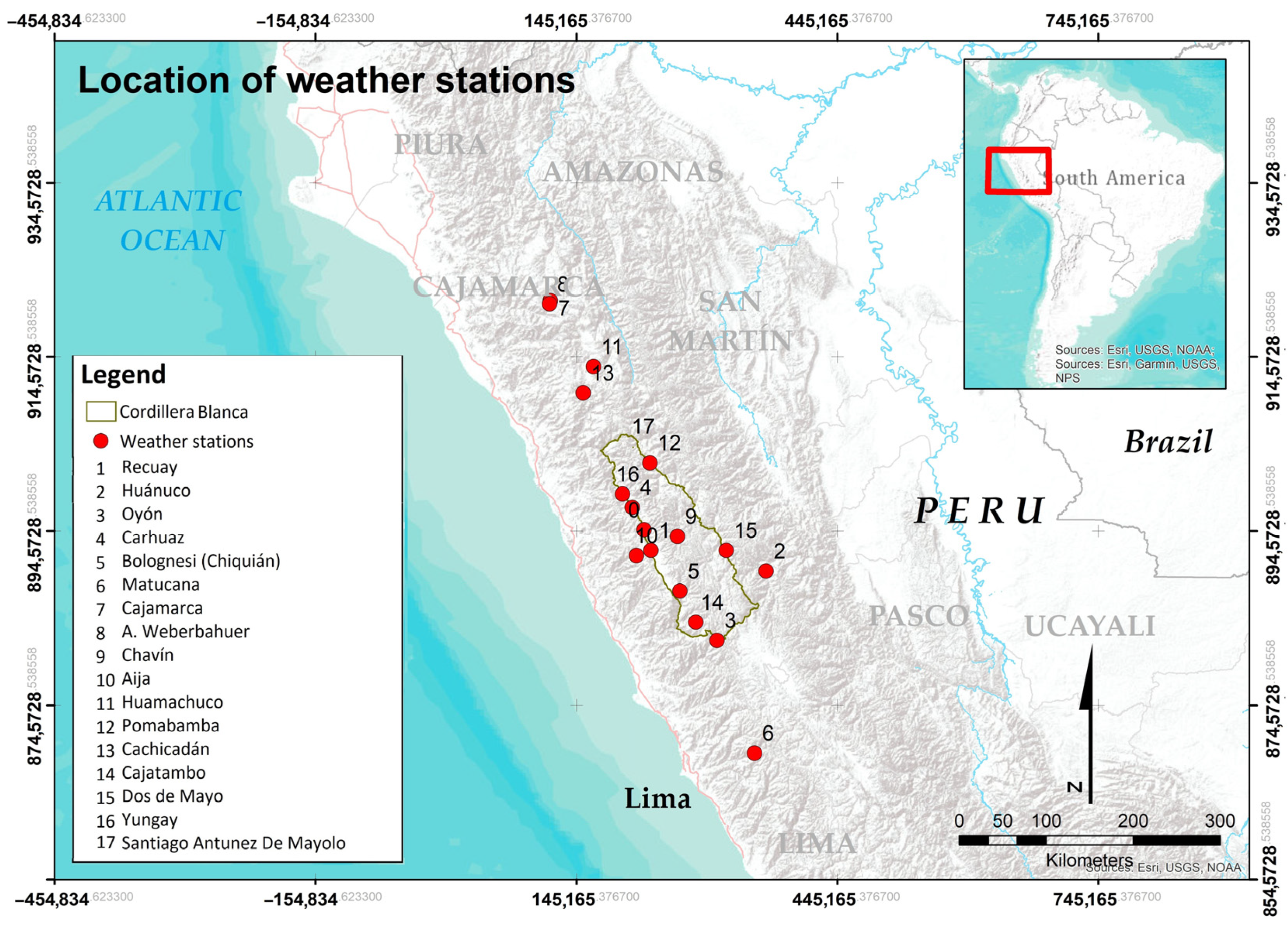
2. Study Area
3. Materials and Methods
3.1. Materials
3.2. Data Series Preprocessing
3.3. Spectral Analysis
4. Results
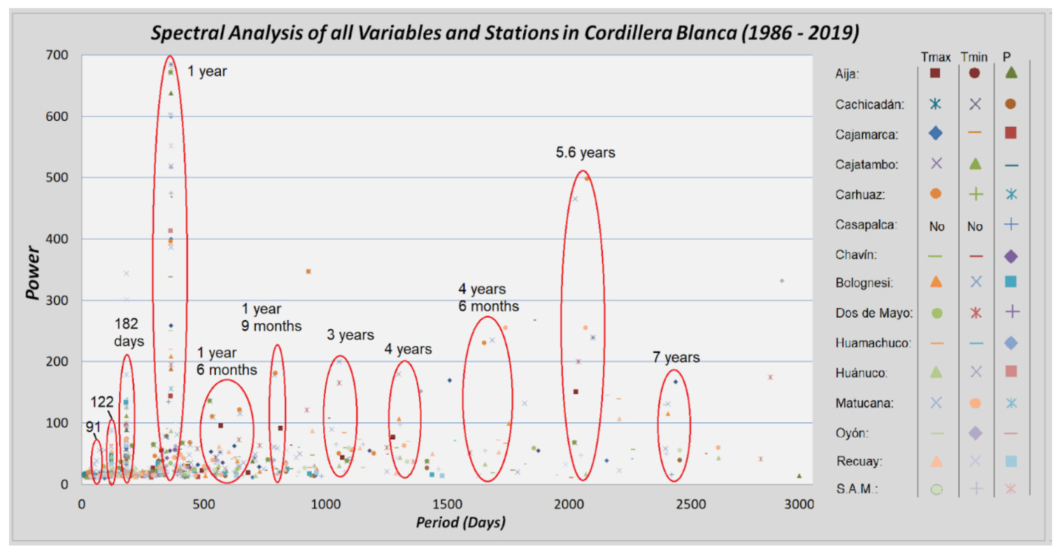
4.1. Analysis of the Spectral Periodicity
- 27 to 30 days (3 months).
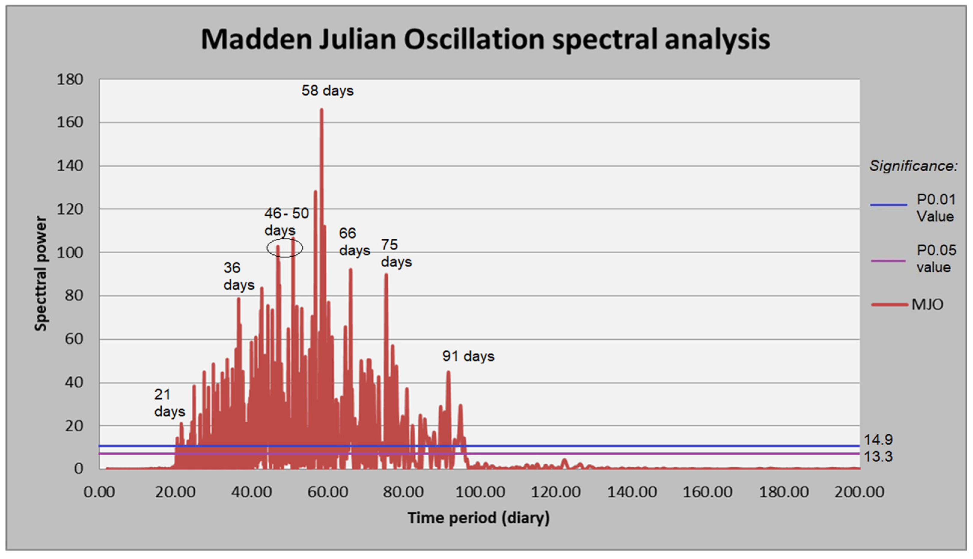
- 46 to 52 days (almost a month and a half).
- 90 days (3 months).
- 479 days (1 years and 3 months).
- Between 548 and 560 days (1 year and 6 months).
- 635 days (1 year and 9 months).
- 1095 days (3 years).
- 1460 days (4 years).
- 1650 days (4.5 years).
- Between 2000 and 2555 days (5.6 to 7 years).
- Between 4015 and 4380 days (11 to 12 years).
- Between 5110 and 6570 days (14 to 18 years).
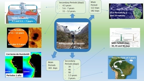
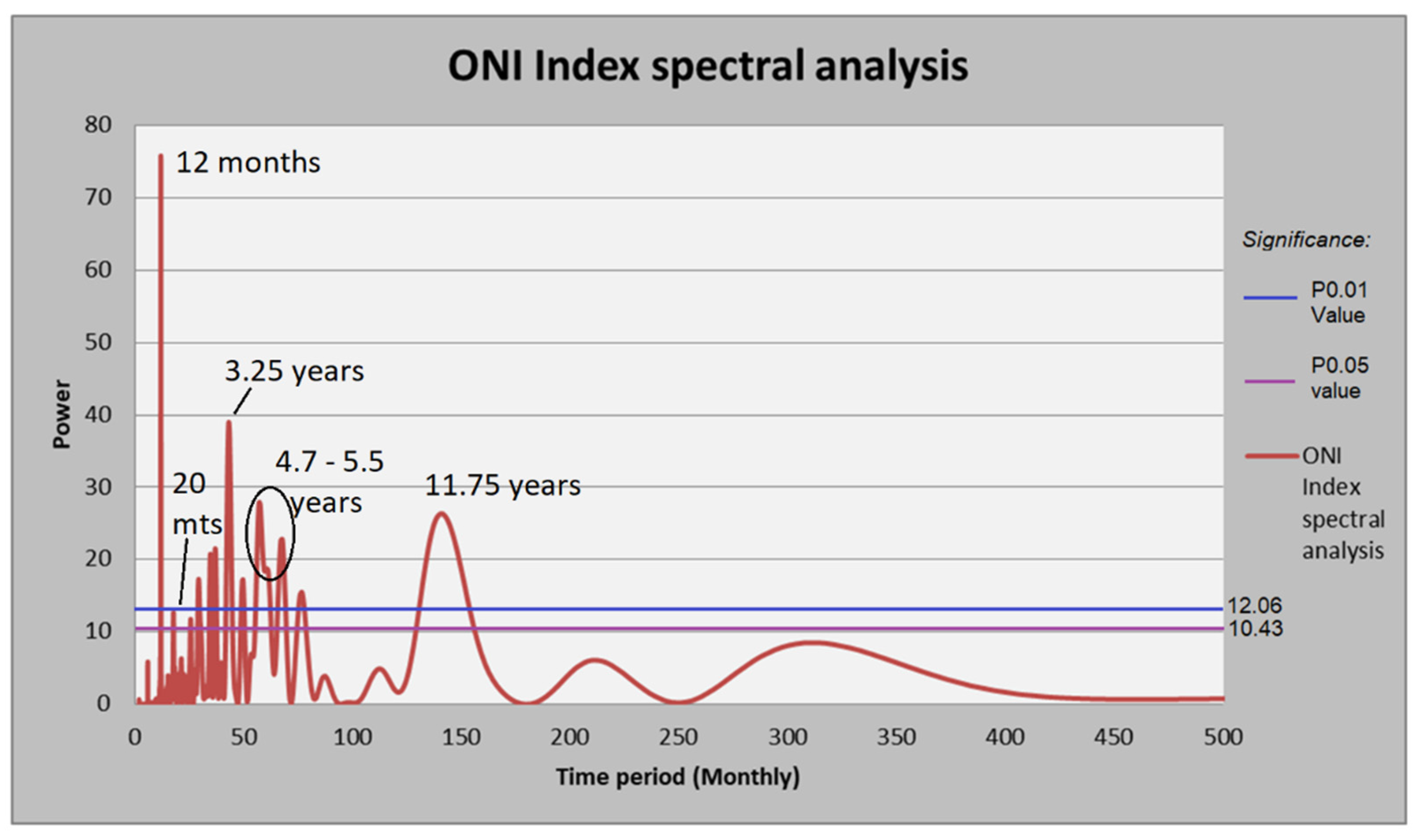
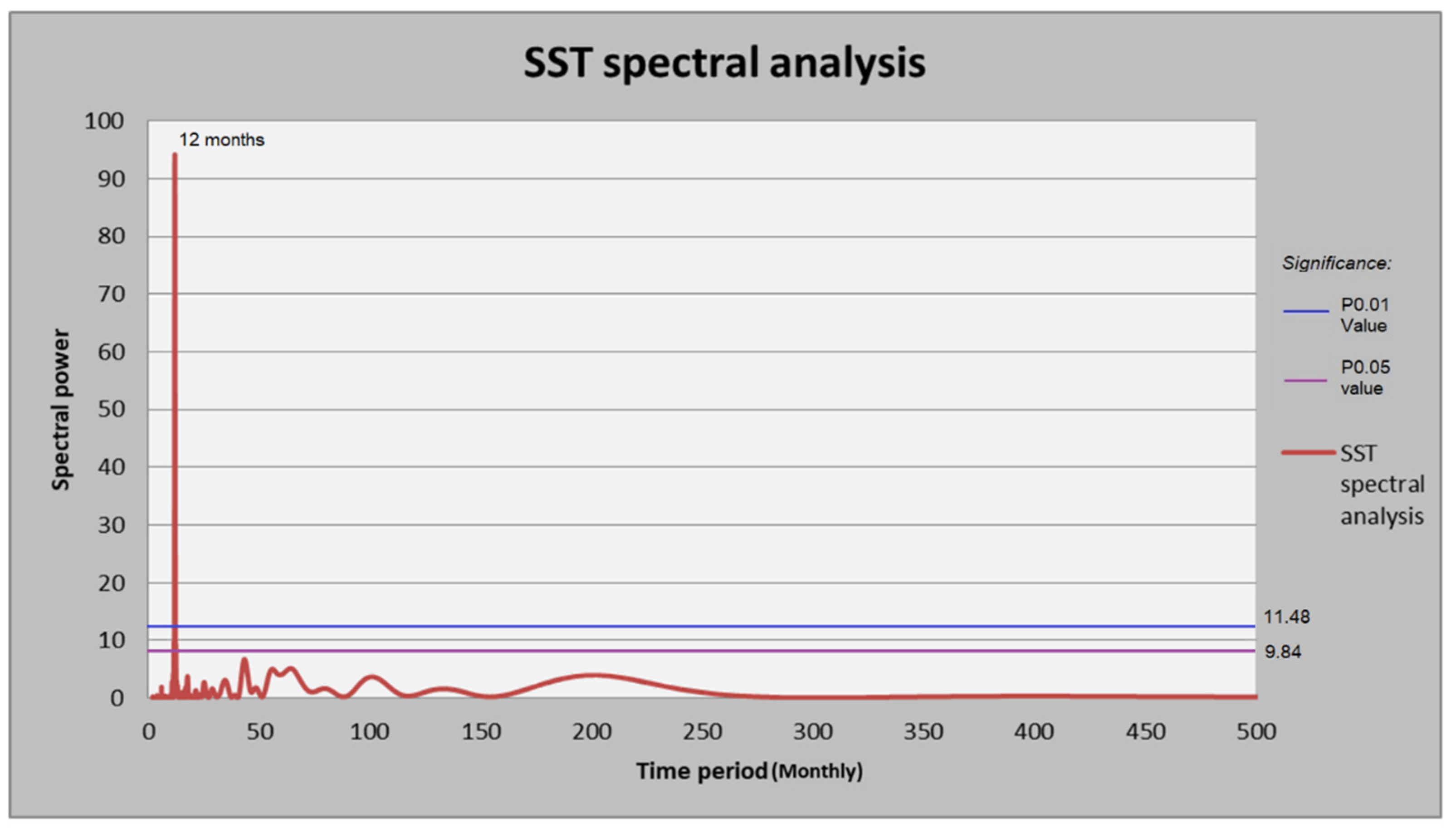
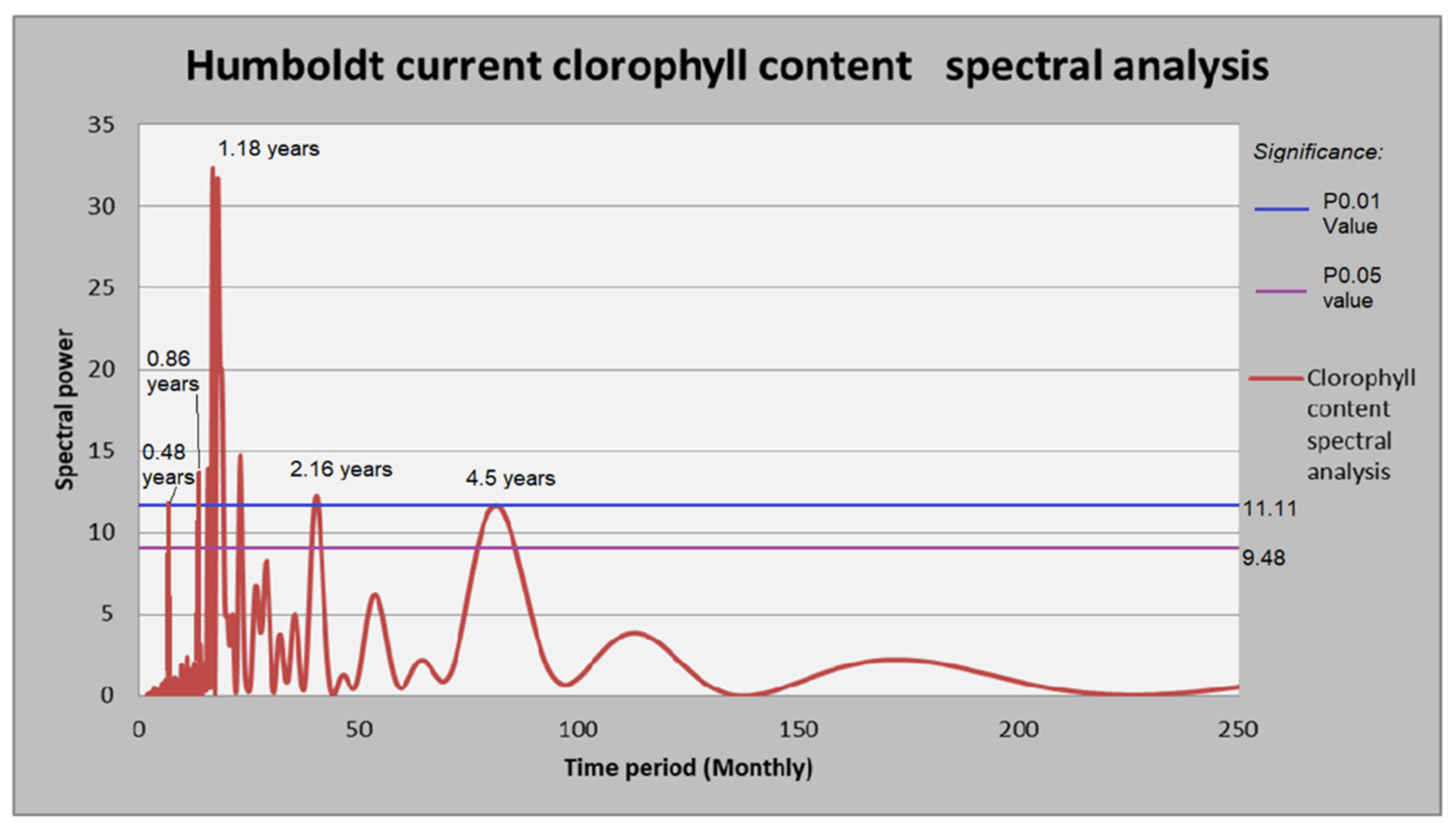
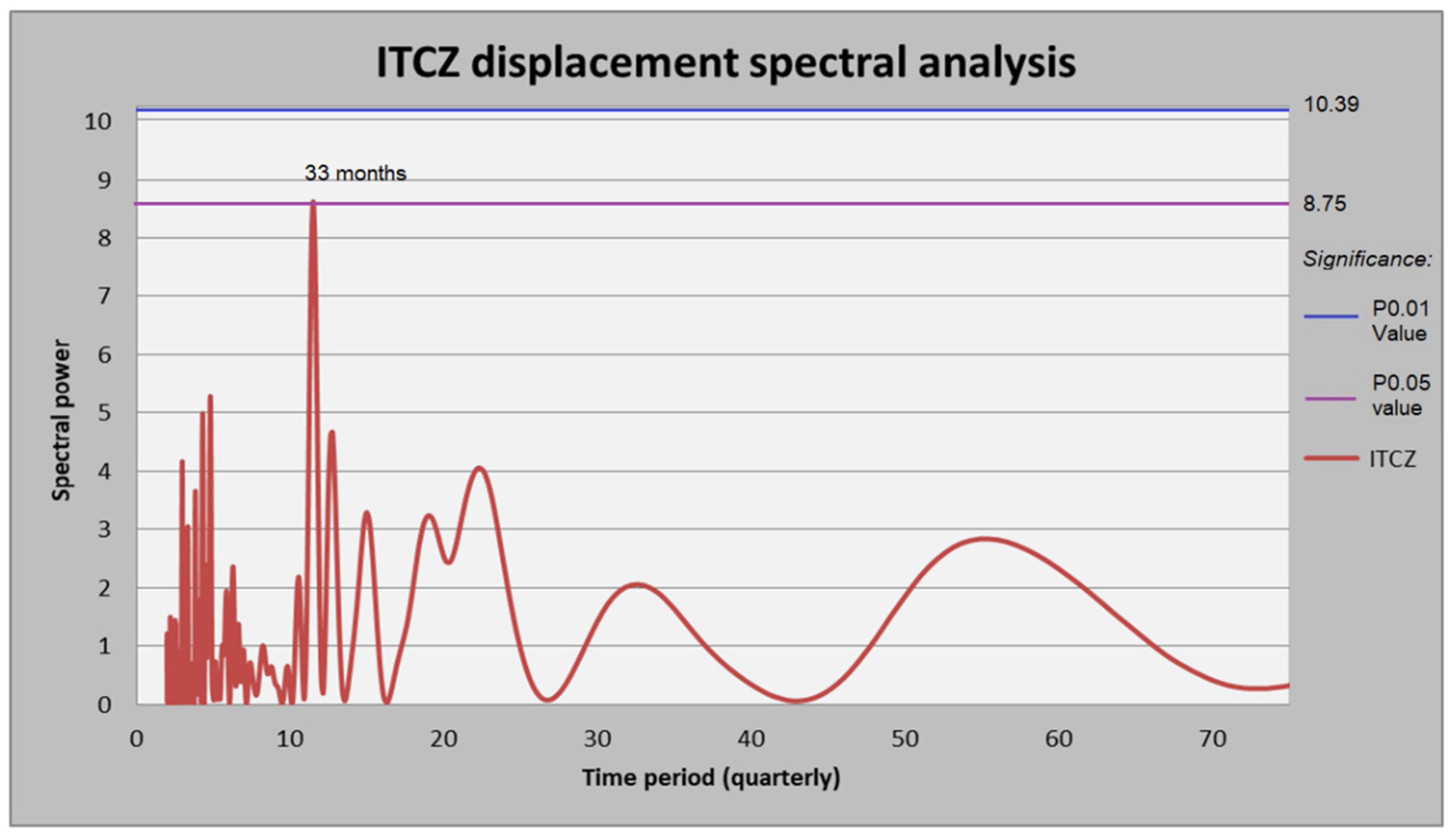
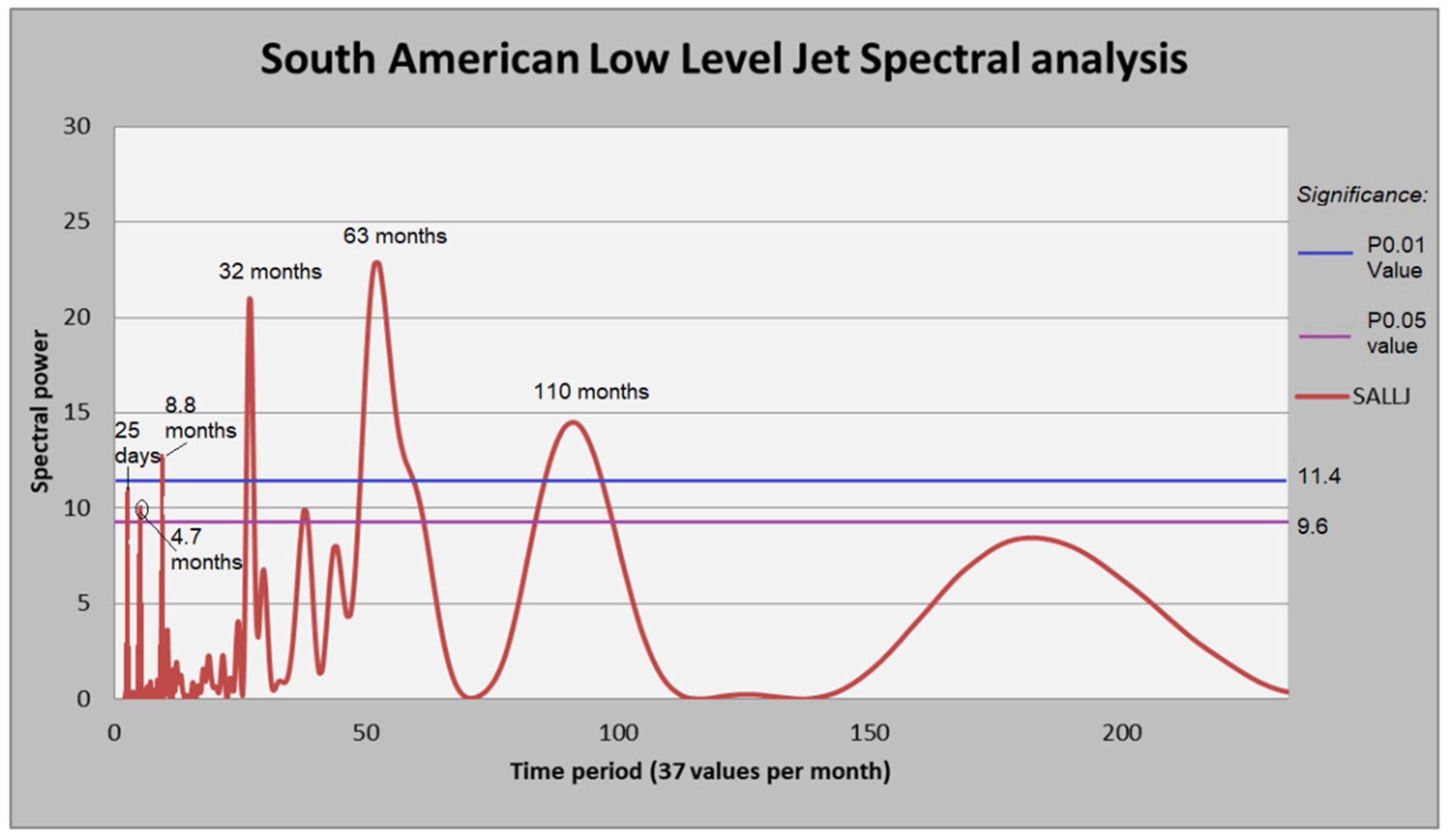
4.2. Spectral Analysis of Main Climatic Patterns
4.3. Results Synthesis
5. Discussion
5.1. Intra-Annual Periodicities
5.2. Interannual Periodicities
5.3. Long Term Periodicities
5.4. Comparison with Other Regions: Cases of Study
5.5. Shortcomings
6. Conclusions
Supplementary Materials
Author Contributions
Funding
Institutional Review Board Statement
Informed Consent Statement
Data Availability Statement
Acknowledgments
Conflicts of Interest
References
- Beer, J.; Mende, W.; Stellmacher, R. The Role of the Sun in Climate Forcing. Quat. Sci. Rev. 2000, 19, 403–415. [Google Scholar] [CrossRef]
- Xiong, Z.; Li, T.; Chang, F.; Algeo, T.J.; Clift, P.D.; Bretschneider, L.; Lu, Z.; Zhu, X.; Frank, M.; Sauer, P.E.; et al. Rapid Precipitation Changes in the Tropical West Pacific Linked to North Atlantic Climate Forcing during the Last Deglaciation. Quat. Sci. Rev. 2018, 197, 288–306. [Google Scholar] [CrossRef]
- Tilmes, S.; Hodzic, A.; Emmons, L.K.; Mills, M.J.; Gettelman, A.; Kinnison, D.E.; Park, M.; Lamarque, J.-F.; Vitt, F.; Shrivastava, M.; et al. Climate Forcing and Trends of Organic Aerosols in the Community Earth System Model (CESM2). J. Adv. Model. Earth Syst. 2019, 11, 4323–4351. [Google Scholar] [CrossRef]
- Richardson, T.B.; Forster, P.M.; Smith, C.J.; Maycock, A.C.; Wood, T.; Andrews, T.; Boucher, O.; Faluvegi, G.; Fläschner, D.; Hodnebrog, Ø.; et al. Efficacy of Climate Forcings in PDRMIP Models. J. Geophys. Res. Atmos. 2019, 124, 12824–12844. [Google Scholar] [CrossRef] [Green Version]
- O’Neel, S.; McNeil, C.; Sass, L.C.; Florentine, C.; Baker, E.H.; Peitzsch, E.; McGrath, D.; Fountain, A.G.; Fagre, D. Reanalysis of the US Geological Survey Benchmark Glaciers: Long-Term Insight into Climate Forcing of Glacier Mass Balance. J. Glaciol. 2019, 65, 850–866. [Google Scholar] [CrossRef] [Green Version]
- Scott, R.C.; Nicolas, J.P.; Bromwich, D.H.; Norris, J.R.; Lubin, D. Meteorological Drivers and Large-Scale Climate Forcing of West Antarctic Surface Melt. J. Clim. 2019, 32, 665–684. [Google Scholar] [CrossRef]
- Takano, Y.; Ito, T.; Deutsch, C. Projected Centennial Oxygen Trends and Their Attribution to Distinct Ocean Climate Forcings. Glob. Biogeochem. Cycles 2018, 32, 1329–1349. [Google Scholar] [CrossRef]
- Garreaud, R.D. The Andes Climate and Weather. Adv. Geosci. 2009, 22, 3–11. [Google Scholar] [CrossRef] [Green Version]
- Veblen, T.; Young, K.; Orme, A. The Physical Geography of South America, 1st ed.; Oxford University Press: New York, NY, USA, 2007; ISBN 978-0-19-531341-3. [Google Scholar]
- Samanta, D.; Karnauskas, K.B.; Goodkin, N.F. Tropical Pacific SST and ITCZ Biases in Climate Models: Double Trouble for Future Rainfall Projections? Geophys. Res. Lett. 2019, 46, 2242–2252. [Google Scholar] [CrossRef] [Green Version]
- Williams, I.N.; Patricola, C.M. Diversity of ENSO Events Unified by Convective Threshold Sea Surface Temperature: A Nonlinear ENSO Index. Geophys. Res. Lett. 2018, 45, 9236–9244. [Google Scholar] [CrossRef]
- IPCC; Arias, P.A.; Allan, R.P.; Armour, K.; Barimalala, R.; Canadell, J.G.; Cassou, C.; Cherchi, A.; Collins, W.; Corti, S.; et al. Climate Change 2021: The Physical Science Basis. Contribution of Working Group I to the Sixth Assessment Report of the Intergovernmental Panel on Climate Change; Intergovernmental Panel on Climate Change: Cambridge, UK; New York, NY, USA, 2021; p. 2409. [Google Scholar]
- Iturbide, M.; Gutiérrez, J.M.; Alves, L.M.; Bedia, J.; Cerezo-Mota, R.; Cimadevilla, E.; Cofiño, A.S.; Di Luca, A.; Faria, S.H.; Gorodetskaya, I.V.; et al. An Update of IPCC Climate Reference Regions for Subcontinental Analysis of Climate Model Data: Definition and Aggregated Datasets. Earth Syst. Sci. Data 2020, 12, 2959–2970. [Google Scholar] [CrossRef]
- IPCC; Stocker, T.F.; Qin, D.; Plattner, G.-K.; Tignor, M.; Allen, S.K.; Boschung, J.; Nauels, A.; Xia, Y.; Bex, V.; et al. Climate Change 2013: The Physical Science Basis. Contribution of Working Group I to the Fifth Assessment Report of the Intergovernmental Panel on Climate Change; Intergovernmental Panel on Climate Change: Cambridge, UK; New York, NY, USA, 2013; p. 1585. [Google Scholar]
- Sulca, J.; Takahashi, K.; Espinoza, J.-C.; Vuille, M.; Lavado-Casimiro, W. Impacts of Different ENSO Flavors and Tropical Pacific Convection Variability (ITCZ, SPCZ) on Austral Summer Rainfall in South America, with a Focus on Peru. Int. J. Climatol. 2018, 38, 420–435. [Google Scholar] [CrossRef]
- Jones, C.; Carvalho, L.M.V. The Influence of the Atlantic Multidecadal Oscillation on the Eastern Andes Low-Level Jet and Precipitation in South America. Npj Clim. Atmospheric. Sci. 2018, 1, 40. [Google Scholar] [CrossRef] [Green Version]
- Cai, W.; McPhaden, M.J.; Grimm, A.M.; Rodrigues, R.R.; Taschetto, A.S.; Garreaud, R.D.; Dewitte, B.; Poveda, G.; Ham, Y.-G.; Santoso, A.; et al. Climate Impacts of the El Niño–Southern Oscillation on South America. Nat. Rev. Earth Environ. 2020, 1, 215–231. [Google Scholar] [CrossRef]
- Bauer, E.; Claussen, M.; Brovkin, V.; Huenerbein, A. Assessing Climate Forcings of the Earth System for the Past Millennium: Climate Simulations for Past Millennium. Geophys. Res. Lett. 2003, 30, 1–9. [Google Scholar] [CrossRef] [Green Version]
- Lomb, N.R. Least-Squares Frequency Analysis of Unequally Spaced Data. Astrophys. Space Sci. 1976, 39, 447–462. [Google Scholar] [CrossRef]
- Zhao, X.; Soon, W.; Velasco Herrera, V.M. Evidence for Solar Modulation on the Millennial-Scale Climate Change of Earth. Universe 2020, 6, 153. [Google Scholar] [CrossRef]
- Zhu, F.R.; Jia, H.Y. Lomb–Scargle Periodogram Analysis of the Periods around 5.5 Year and 11 Year in the International Sunspot Numbers. Astrophys. Space Sci. 2018, 363, 138. [Google Scholar] [CrossRef]
- Pezzopane, M.; Pignalberi, A.; Pietrella, M. On the Influence of Solar Activity on the Mid-Latitude Sporadic E Layer. J. Space Weather Space Clim. 2015, 5, A31. [Google Scholar] [CrossRef] [Green Version]
- Akdi, Y.; Gölveren, E.; Ünlü, K.D.; Yücel, M.E. Modeling and Forecasting of Monthly PM2.5 Emission of Paris by Periodogram-Based Time Series Methodology. Environ. Monit. Assess. 2021, 193, 622. [Google Scholar] [CrossRef] [PubMed]
- Aldegunde, J.A.Á.; Fernández-Sánchez, A.; Saba, M.; Bolaños, E.Q.; Caraballo, L.R. Spatiotemporal Analysis of PM2.5 Concentrations on the Incidence of Childhood Asthma in Developing Countries: Case Study of Cartagena de Indias, Colombia. Atmosphere 2022, 13, 1383. [Google Scholar] [CrossRef]
- Froyland, G.; Giannakis, D.; Lintner, B.R.; Pike, M.; Slawinska, J. Spectral Analysis of Climate Dynamics with Operator-Theoretic Approaches. Nat. Commun. 2021, 12, 6570. [Google Scholar] [CrossRef] [PubMed]
- Akdi, Y.; Ünlü, K.D. Periodicity in Precipitation and Temperature for Monthly Data of Turkey. Theor. Appl. Climatol. 2021, 143, 957–968. [Google Scholar] [CrossRef]
- Lamy, F.; Hebbeln, D.; Röhl, U.; Wefer, G. Holocene Rainfall Variability in Southern Chile: A Marine Record of Latitudinal Shifts of the Southern Westerlies. Earth Planet. Sci. Lett. 2001, 185, 369–382. [Google Scholar] [CrossRef]
- Warner, R.M.; Neumann, P.G. SPAN: An Interactive BASIC Program for Spectral Analysis of Time-Series Data. Behav. Res. Methods Instrum. 1980, 12, 389–390. [Google Scholar] [CrossRef] [Green Version]
- Fernández-Sánchez, A.; Martín-Chivelet, J. Revisión de la estratigrafía del δ 18 O en sondeos de hielo de glaciares de los Andes Centrales: Implicaciones para la variabilidad climática del Holoceno. In Proceedings of the Geotemas, Huelva, Spain, 12–14 September 2016; Volume 16, pp. 565–568. [Google Scholar]
- Canedo-Rosso, C.; Uvo, C.B.; Berndtsson, R. Precipitation Variability and Its Relation to Climate Anomalies in the Bolivian Altiplano. Int. J. Climatol. 2018, 39, 2096–2107. [Google Scholar] [CrossRef] [Green Version]
- Ilyes, C.; Wendo, V.A.J.A.; Flores Carpio, Y.; Szucs, P. Differences and Similarities between Precipitation Patterns of Different Climates. Acta Geod. Geophys. 2021, 56, 781–800. [Google Scholar] [CrossRef]
- Eguiguren-Velepucha, P.A.; Chamba, J.A.M.; Aguirre Mendoza, N.A.; Ojeda-Luna, T.L.; Samaniego-Rojas, N.S.; Furniss, M.J.; Howe, C.; Aguirre Mendoza, Z.H. Tropical Ecosystems Vulnerability to Climate Change in Southern Ecuador. Trop. Conserv. Sci. 2016, 9, 194008291666800. [Google Scholar] [CrossRef] [Green Version]
- Deb, J.; Phinn, S.; Butt, N.; McAlpine, C. Climate Change Impacts on Tropical Forests. For. Res. Inst. Malays. 2018, 30, 182–194. [Google Scholar]
- INAIGEM. Informe de la Situación de los Glaciares y Ecosistemas de Montaña en el Perú; Instituto Nacional de Investigación en Glaciares y Ecosistemas de Montaña del Perú: Huaraz, Peru, 2017; p. 124. [Google Scholar]
- Ames Marquez, A.; Francou, B. Cordillera Blanca: Glaciares En La Historia. Bull. Inst. Fr. Etudes Andin. 1995, 24, 37–64. [Google Scholar] [CrossRef]
- SENAMHI. Climas del Perú: Mapa de Clasificación Climática Nacional; Servicio Nacional de Meteorología e HIdrología del Perú: Lima, Peru, 2020; p. 70. [Google Scholar]
- Kaser, G.; Osmaston, H. Tropical Glaciers, 1st ed.; International Hydrology Series; Cambridge University Press: Cambridge, UK, 2002; ISBN 0-521-63333-8. [Google Scholar]
- Autoridad Nacional del Agua; Unidad de Glaciología y Recursos Hídricos. Inventario nacional de glaciares y lagunas: Lagunas; Autoridad Nacional del Agua: Huaraz, Peru, 2014; p. 21. [Google Scholar]
- Instituto Nacional de Estadística e Informática. INEI Censo de Población y Vivienda: Ancash. 2018. Available online: www.inei.gob.pe (accessed on 3 December 2022).
- Cano, A.; Mendoza, W.; Castillo, S.; Morales, M.; La Torre, M.I.; Aponte, H.; Delgado, A.; Valencia, N.; Vega, N. Flora y vegetación de suelos crioturbados y hábitats asociados en la Cordillera Blanca, Ancash, Perú. Rev. Peru. Biol. 2011, 17, 095–0103. [Google Scholar] [CrossRef]
- NOAA Oceanic El NIño Index. Available online: https://www.cpc.ncep.noaa.gov/data/indices/oni.ascii.txt (accessed on 20 February 2022).
- Huang, X.; Zhou, T.; Dai, A.; Li, H.; Li, C.; Chen, X.; Lu, J.; Von Storch, J.-S.; Wu, B. South Asian Summer Monsoon Projections Constrained by the Interdecadal Pacific Oscillation. Sci. Adv. 2020, 6, eaay6546. [Google Scholar] [CrossRef] [Green Version]
- Marrari, M.; Piola, A.R.; Valla, D. Variability and 20-Year Trends in Satellite-Derived Surface Chlorophyll Concentrations in Large Marine Ecosystems around South and Western Central America. Front. Mar. Sci. 2017, 4, 372. [Google Scholar] [CrossRef] [Green Version]
- Hidalgo, H.G.; Durán-quesada, A.M.; Amador, J.A.; Alfaro, E.J. The Caribbean Low-level Jet, the Inter-tropical Convergence Zone and Precipitation Patterns in the Intra-americas Sea: A Proposed Dynamical Mechanism. Geogr. Ann. Ser. Phys. Geogr. 2015, 97, 41–59. [Google Scholar] [CrossRef]
- Lee, H.-T. NOAA CDR Program NOAA Climate Data Record (CDR) of Daily Outgoing Longwave Radiation (OLR), Version 1.2 . 2014. [Google Scholar]
- Reason, C.J.C. The Bolivian, Botswana, and Bilybara Highs and Southern Hemisphere Drought/Floods. Geophys. Res. Lett. 2016, 43, 1280–1286. [Google Scholar] [CrossRef]
- Jones, C. Recent Changes in the South America Low-Level Jet. Npj Clim. Atmos. Sci. 2019, 2, 20. [Google Scholar] [CrossRef] [Green Version]
- Sierra, J.P.; Arias, P.A.; Durán-Quesada, A.M.; Tapias, K.A.; Vieira, S.C.; Martínez, J.A. The Choco Low-level Jet: Past, Present and Future. Clim. Dyn. 2021, 56, 2667–2692. [Google Scholar] [CrossRef]
- Xue, Y.; Higgins, W.; Kousky, V. Influences of the Madden Julian Oscillations on Temperature and Precipitation in North America during ENSO-Neutral and Weak ENSO Winters. In Proc. Workshop on Prospects for Improved Forecasts of Weather and Short-Term Climate Variability on Subseasonal (2 Week to 2 Month) Time Scales; NASA/Goddard Space Flight Center: Greenbelt, MD, USA, 2002; p. 4. [Google Scholar]
- Polanco Martínez, J. Aplicación de Técnicas Estadísticas en el Estudio de Fenómenos Ambientales y Ecosistémicos; Universidad del País Vasco, Facultad de Ciencia y Tecnología, Departamento de Física Aplicada II. Leioa: Vizcaya, Spain, 2011. [Google Scholar]
- Paulhus, J.L.H.; Kohler, M.A. Interpolation of Missing Precipitation Records. Mon. Weather Rev. 1952, 80, 129–133. [Google Scholar] [CrossRef]
- Enders, C.K. Methodology in the social sciences. In Applied Missing Data Analysis, 1st ed.; Guilford Press: New York, NY, USA, 2010; ISBN 978-1-60623-639-0. [Google Scholar]
- RStudio Team. Integrated Development for R, PBC; RStudio Team: Boston, MA, USA, 2020; Available online: http://www.rstudio.com/ (accessed on 1 July 2021).
- James, G.; Written, D.; Hastie, T.; Tibshirani, R. An Introduction to Statistical Learning with Applications in R, 2nd ed.; Springer Science and Business Media: New York, NY, USA, 2021; Volume 6, ISBN 978-1-07-161417-4. [Google Scholar]
- Warner, R.M. Spectral Analysis of Time-Series Data (Methodology in the Social Sciences), 1st ed.; Guilford Press: New York, USA, 1999; ISBN 978-1-57230-338-6. [Google Scholar]
- Li, L.; Li, K.; Liu, C.; Liu, C. Comparison of Detrending Methods in Spectral Analysis of Heart Rate Variability. Res. J. Appl. Sci. Eng. Technol. 2011, 3, 1014–1021. [Google Scholar]
- Hammer, O.; Harper, D.A.T.; Ryan, P.D. PAST: Paleontological Statistics Software Package for Education and Data Analysis. Palaeontol. Electron. 2001, 4, 9. [Google Scholar]
- Miyahara, H.; Aono, Y.; Kataoka, R. Searching for the 27-Day Solar Rotational Cycle in Lightning Events Recorded in Old Diaries in Kyoto from the 17th to 18th Century. Ann. Geophys. 2017, 35, 1195–1200. [Google Scholar] [CrossRef]
- Lin, Y.; Yu, J.; Wu, C.; Zheng, F. The Footprint of the 11-Year Solar Cycle in Northeastern Pacific SSTs and Its Influence on the Central Pacific El Niño. Geophys. Res. Lett. 2021, 48, e2020GL091369. [Google Scholar] [CrossRef]
- Maruyama, F.; Kai, K.; Morimoto, H. Wavelet-Based Multifractal Analysis on a Time Series of Solar Activity and PDO Climate Index. Adv. Space Res. 2017, 60, 1363–1372. [Google Scholar] [CrossRef]
- SENAMHI. Escenarios del Cambio Climático en el Perú al 2050: Cuenca del Río Piura; Servicio Nacional de Meteorología e HIdrología del Perú: Lima, Peru, 2005; p. 197. [Google Scholar]
- Gutiérrez, D.; Akester, M.; Naranjo, L. Productivity and Sustainable Management of the Humboldt Current Large Marine Ecosystem under Climate Change. Environ. Dev. 2016, 17, 126–144. [Google Scholar] [CrossRef]
- Xie, X.; Zhou, S.; Zhang, J.; Huang, P. The Role of Background SST Changes in the ENSO-Driven Rainfall Variability Revealed from the Atmospheric Model Experiments in CMIP5/6. Atmos. Res. 2021, 261, 105732. [Google Scholar] [CrossRef]
- Mamalakis, A.; Randerson, J.T.; Yu, J.-Y.; Pritchard, M.S.; Magnusdottir, G.; Smyth, P.; Levine, P.A.; Yu, S.; Foufoula-Georgiou, E. Zonally Contrasting Shifts of the Tropical Rain Belt in Response to Climate Change. Nat. Clim. Change 2021, 11, 143–151. [Google Scholar] [CrossRef] [PubMed]
- Montini, T.L.; Jones, C.; Carvalho, L.M.V. The South American Low-Level Jet: A New Climatology, Variability, and Changes. J. Geophys. Res. Atmos. 2019, 124, 1200–1218. [Google Scholar] [CrossRef]
- Alvarez, M.; Vera, C.S.; Kiladis, G.; Liebmann, B. Influence of the Madden Julian Oscillation on Precipitation and Surface Air Temperature in South America. Clim. Dyn. 2015, 46, 245–262. [Google Scholar] [CrossRef]
- Alvarez, M.; Vera, C.; Kiladis, G. MJO Modulating the Activity of the Leading Mode of Intraseasonal Variability in South America. Atmosphere 2017, 8, 232. [Google Scholar] [CrossRef] [Green Version]
- Grimm, A.M. Interannual Climate Variability in South America: Impacts on Seasonal Precipitation, Extreme Events, and Possible Effects of Climate Change. Stoch. Environ. Res. Risk Assess. 2011, 25, 537–554. [Google Scholar] [CrossRef]
- Cess, R.D.; Zhang, M.; Wielicki, B.A.; Young, D.F.; Zhou, X.-L.; Nikitenko, Y. The Influence of the 1998 El Niño upon Cloud-Radiative Forcing over the Pacific Warm Pool. J. Clim. 2001, 14, 2129–2137. [Google Scholar] [CrossRef]
- Song, Z.; Liu, H.; Chen, X. Eastern Equatorial Pacific SST Seasonal Cycle in Global Climate Models: From CMIP5 to CMIP6. Acta Oceanol. Sin. 2020, 39, 50–60. [Google Scholar] [CrossRef]
- Carrillo, C.M. The Rainfall over Tropical South America Generated by Multiple Scale Processes. Master’s Thesis, Iowa State University, Digital Repository, Ames, IA, USA, 2010; p. 2807786. [Google Scholar]
- Huang, Y.; Ramaswamy, V.; Soden, B. An Investigation of the Sensitivity of the Clear-Sky Outgoing Longwave Radiation to Atmospheric Temperature and Water Vapor. J. Geophys. Res. Atmos. 2007, 112, 13. [Google Scholar] [CrossRef]
- Kluft, L.; Dacie, S.; Brath, M.; Buehler, S.; Stevens, B. Temperature-Dependence of the Clear-Sky Feedback in Radiative-Convective Equilibrium. Geophys. Res. Lett. 2021, 48, 10. [Google Scholar] [CrossRef]
- Lu, B.; Jin, F.-F.; Ren, H.-L. A Coupled Dynamic Index for ENSO Periodicity. J. Clim. 2018, 31, 16. [Google Scholar] [CrossRef]
- Su, H.; Jiang, J.; Neelin, D.; Shen, J.; Zhai, C.; Yue, Q.; Wang, Z.; Huang, L.; Choi, Y.-S.; Stephens, G.; et al. Tightening of Tropical Ascent and High Clouds Key to Precipitation Change in a Warmer Climate. Nat. Commun. 2017, 8, 9. [Google Scholar] [CrossRef] [Green Version]
- Hathaway, D.H. The Solar Cycle. Living Rev. Sol. Phys. 2015, 12, 4. [Google Scholar] [CrossRef]
- Chowdhury, P.; Choudhary, D.P.; Gosain, S.; Moon, Y.-J. Short-Term Periodicities in Interplanetary, Geomagnetic and Solar Phenomena during Solar Cycle 24. Astrophys. Space Sci. 2015, 356, 7–18. [Google Scholar] [CrossRef]
- Chowdhury, P.; Dwivedi, B.N. Periodicities of Sunspot Number and Coronal Index Time Series During Solar Cycle 23. Sol. Phys. 2011, 270, 365–383. [Google Scholar] [CrossRef]
- Feliks, Y.; Small, J.; Ghil, M. Global Oscillatory Modes in High-end Climate Modeling and Reanalyses. Clim. Dyn. 2021, 57, 3385–3411. [Google Scholar] [CrossRef]
- Martín-Chivelet, J. Cambios Climáticos: Una Aproximación al Sistema Tierra.; Fondo de Cultura Económica: Madrid, Spain, 1999; Volume 1, ISBN 84-7954-542-9. [Google Scholar]
- Griggs, J.A.; Harries, J.E. Comparison of Spectrally Resolved Outgoing Longwave Data between 1970 and Present; Strojnik, M., Ed.; University of Bristol: Denver, CO, USA, 2004; p. 164. [Google Scholar]
- Koll, D.D.B.; Cronin, T.W. Earth’s Outgoing Longwave Radiation Linear Due to H2O Greenhouse Effect. Proc. Natl. Acad. Sci. USA 2018, 115, 10293–10298. [Google Scholar] [CrossRef] [Green Version]
- Manabe, S. Role of Greenhouse Gas in Climate Change. Tellus Dyn. Meteorol. Oceanogr. 2019, 71, 1620078. [Google Scholar] [CrossRef] [Green Version]
- Zhang, L.; Delworth, T.L. Simulated Response of the Pacific Decadal Oscillation to Climate Change. J. Clim. 2016, 29, 5999–6018. [Google Scholar] [CrossRef]
- Kayano, M.T.; Andreoli, R.V. Relations of South American Summer Rainfall Interannual Variations with the Pacific Decadal Oscillation. Int. J. Climatol. 2007, 27, 531–540. [Google Scholar] [CrossRef]
- Gamelin, B.L.; Carvalho, L.M.V.; Jones, C. Evaluating the Influence of Deep Convection on Tropopause Thermodynamics and Lower Stratospheric Water Vapor: A RELAMPAGO Case Study Using the WRF Model. Atmos. Res. 2022, 267, 105986. [Google Scholar] [CrossRef]
- Reboita, M.S.; Ambrizzi, T.; Crespo, N.M.; Dutra, L.M.M.; Ferreira, G.W.d.S.; Rehbein, A.; Drumond, A.; da Rocha, R.P.; Souza, C.A. de Impacts of Teleconnection Patterns on South America Climate. Ann. N. Y. Acad. Sci. 2021, 1504, 116–153. [Google Scholar] [CrossRef]
- Wang, Y.-L.; Hsu, Y.-C.; Lee, C.-P.; Wu, C.-R. Coupling Influences of ENSO and PDO on the Inter-Decadal SST Variability of the ACC around the Western South Atlantic. Sustainability 2019, 11, 4853. [Google Scholar] [CrossRef] [Green Version]
- Herho, S.; Fajary, F.; Irawan, D. On the Statistical Learning Analysis of Rain Gauge Data over the Natuna Islands. Indones. J. Stat. Its Appl. 2022, 6, 347–357. [Google Scholar] [CrossRef]
- Nogués-Paegle, J.; Mechoso, C.R.; Fu, R.; Berbery, E.H.; Chao, W.C.; Chen, T.-C.; Cook, K.; Diaz, A.F.; Enfield, D.; Ferreira, R.; et al. Progress in Panamerican Clivar Research: Understanding the South American Monsoon System. Meteorologica 2002, 27, 3–32. [Google Scholar]
- WMO. State of the Climate in Latin America and the Caribbean 2021; World Meteorological Organization: Geneva, Switzerland, 2021; p. 44. [Google Scholar]


| Weather Stations | Chosen Period | Variable | Altitude (m.a.s.l) |
|---|---|---|---|
| Aija | 1999–2019 | P., Max. T, Min.T. | 3478 |
| Cachicadan | 1986–2019 | P., Max. T, Min.T. | 2885 |
| Cajamarca | 1986–2019 | P., Max. T, Min.T. | 2686 |
| Cajatambo | 1990–2019 | P., Max. T, Min.T. | 3405 |
| Casapalca | 1987–2019 | Precipitation | 4924 |
| Carhuaz | 1986–2016 | P., Max. T, Min.T. | 2644 |
| Chavín | 2000–2019 | P., Max. T, Min.T. | 3132 |
| Chiquián | 1986–2019 | P., Max. T, Min.T. | 3412 |
| Dos de Mayo | 2000–2019 | P., Max. T, Min.T. | 3474 |
| Huamachuco | 1986–2019 | P., Max. T, Min.T. | 3178 |
| Huánuco | 1986–2019 | P., Max. T, Min.T. | 1918 |
| Matucana | 1986–2019 | P., Max. T, Min.T. | 2417 |
| Oyón | 1986–2019 | P., Max. T, Min.T. | 3663 |
| Pomabamba | 1989–2019 | P., Max. T, Min.T. | 2975 |
| A. Weberbahuer | 1986–2019 | P., Max. T, Min.T. | 2666 |
| Huaraz | 1998–2019 | P., Max. T, Min.T. | 3071 |
| Recuay | 1986–2019 | P., Max. T, Min.T. | 3417 |
| Index | Region | Period |
|---|---|---|
| ONI Index (ENSO) [41] | Equatorial Pacific | 1950–2021 |
| SST Index [42] | El Niño 1 + 2 | 1982–2021 |
| Humboldt Current [43] | 7–9° S latitude | 1997–2017 |
| ITCZ displacement [44] | 90–60° W longitude | 1979–2005 |
| Outgoing Longwave Radiation [45] | Peruvian Andes | 1999–2014 |
| Bolivian High [46] | Bolivia | 1979–2014 |
| SALLJ [47] | Eastern Andes | 1979–2018 |
| Chocó LLJ [48] | Colombia North | 1978–2010 |
| Caribbean LLJ [44] | Caribbean Sea | 1979–2010 |
| MJO Index [49] | 40° W longitude | 1979–2021 |
| Variable | Intraseasonal | Intraseasonal | Intraseasonal | Interseasonal | Interseasonal | Annual |
|---|---|---|---|---|---|---|
| Maximum T. | 27–30 days | 46–52 days | 90 days | 122 days | 182 days | 365 days |
| Minimum T. | 27–30 days | 46–52 days | 90 days | 122 days | 182 days | 365 days |
| Precipitation | No period | 46–52 days | 90 days | 122 days | 182 days | 365 days |
| Variable | Interannual | Interannual | Interannual | Interannual | Interannual | Interannual | Interdec. | Interdec. |
|---|---|---|---|---|---|---|---|---|
| Maximum T. | 1 yr 3 m. | 1 yr 6 m. | 1 yr 9 m. | 3 yr | 4 yr 6 m | 5.6–7 yr | 11–12 yr | 14–18 yr |
| Minimum T. | 1 yr 3 m. | 1 yr 6 m. | 1 yr 9 m. | 3 yr | 4 yr 6 m | 5.6–7 yr | 11–12 yr | No period |
| Precipitation | No period | 1 yr 3 m. | 1 yr 9 m. | No period | No period | 5.6–7 yr | 11–12 yr | 14–18 yr |
Publisher’s Note: MDPI stays neutral with regard to jurisdictional claims in published maps and institutional affiliations. |
© 2022 by the authors. Licensee MDPI, Basel, Switzerland. This article is an open access article distributed under the terms and conditions of the Creative Commons Attribution (CC BY) license (https://creativecommons.org/licenses/by/4.0/).
Share and Cite
Fernández-Sánchez, A.; Úbeda, J.; Tanarro, L.M.; Naranjo-Fernández, N.; Álvarez-Aldegunde, J.A.; Iparraguirre, J. Climate Patterns and Their Influence in the Cordillera Blanca, Peru, Deduced from Spectral Analysis Techniques. Atmosphere 2022, 13, 2107. https://doi.org/10.3390/atmos13122107
Fernández-Sánchez A, Úbeda J, Tanarro LM, Naranjo-Fernández N, Álvarez-Aldegunde JA, Iparraguirre J. Climate Patterns and Their Influence in the Cordillera Blanca, Peru, Deduced from Spectral Analysis Techniques. Atmosphere. 2022; 13(12):2107. https://doi.org/10.3390/atmos13122107
Chicago/Turabian StyleFernández-Sánchez, Adrián, José Úbeda, Luis Miguel Tanarro, Nuria Naranjo-Fernández, José Antonio Álvarez-Aldegunde, and Joshua Iparraguirre. 2022. "Climate Patterns and Their Influence in the Cordillera Blanca, Peru, Deduced from Spectral Analysis Techniques" Atmosphere 13, no. 12: 2107. https://doi.org/10.3390/atmos13122107