The Role of Phytoplankton Biomacromolecules in Controlling Ocean Surface Roughness

Abstract

Satellite altimetric data routinely map sea surface topography by measuring the ocean return signal. One source of altimeter measurement contamination occurs when the radar ocean backscatter becomes unusually large, a situation termed a Sigma-0 bloom. Past research suggests Sigma-0 blooms are associated with weak wind and natural surface slick conditions where capillary waves at the air–sea interface are suppressed. To date, no explicit connection between these conditions and Sigma-0 bloom presence has been provided. Using a series of simplified equations, our reduced model determines capillary wave heights from estimates of planktonic carbon concentrations and regional wind speed. Our results suggest that the radar signal reflection increases as capillary wave height decreases. This relationship depends on surfactant concentration, surfactant composition, and wind speed. Model sensitivity analysis indicates that the interface reflectivity depends on biological activity and wind speed. Our proposed simplified model provides a method to identify potential Sigma-0 bloom regions. We conclude that because of the demonstrated impact of biological surfactants on ocean roughness, it is necessary to consider the biological activity, i.e., phytoplankton bloom events, when interpreting signals from radar altimetry and when developing ocean hydrology models.

1. Introduction

1.1. Measuring Sea Surface Height with Satellites

Changes in the surface topography of the ocean are now routinely used to monitor ocean circulation dynamics and sea level rise. Satellite altimeters provide these data by measuring the return signal from a radar pulse [1]. Radar signals in the microwave range are transmitted toward the ocean, and the time taken for them to travel from the satellite antenna to the water surface and back is calculated. The return signal (waveform) also provides a time evolution of reflected power, from which the range parameter (i.e., satellite to surface distance) is extracted. The waveform shape and amplitude depend strongly on the local roughness of the ocean surface. Radar altimetry thus also provides an estimate for the backscattering cross-section (Sigma-0, σ⁰), or the proportion of the radiation that is returned in the direction of the incident signal. The strength of the return depends on the roughness of the surface and the wavelength of incidence [2].

At times, across the global ocean, regions have been found to exhibit unusually high values for Sigma-0. These localized phenomena are referred to as Sigma-0 blooms. Altimeter Sigma-0 blooms, and their high backscattering tendency, indicate that the sea surface has become smooth and is thus acting more as a specular reflector than a scattering boundary with respect to the incident electromagnetic radar signal. These Sigma-0 bloom cases can be thought of as a contamination of the radar return signal because they can cause a breakdown in the basic assumptions required to estimate surface height from the return power signal [3,4]. The phenomenon impacts a significant portion of satellite-derived wave height data, and thus the overall success of the radar altimetry method. During the historic TOPEX/Poseidon joint altimeter mission approximately 5–10% of the altimeter data were affected by the presence of Sigma-0 blooms. Yet, this potential error source is often not considered during analysis [3,5]. Efforts to explore mechanisms and reasons behind the reflected Sigma-0 blooms might, at the very least, help to mitigate such contamination in sea surface height mapping [6].

1.2. Sigma-0 Blooms and Capillary Waves

A likely general explanation for Sigma-0 bloom events is that they are associated with seawater surfaces with damped capillary waves, i.e., smooth interfaces [7]. Even the largest planetary ocean wind waves start as tiny capillary waves in the ocean microlayer, the upper 1000 micrometers of the water column. These waves, of very short wavelength, arise when surface wind stress induces small vortices in a completely flat sea. As these small capillary ripples propagate and develop turbulent eddies, the waves grow and become gravity waves. Capillary waves act as the “fastening system” of the sea-air interface, providing the opportunity for wind to exert friction. As such, they govern momentum transfer from atmospheric forcing. However, what is most critical to this study is the fact that capillary wave dynamics are also controlled by the surface tension of the ocean’s microlayer.

1.3. Biological Impact on Surface Tension

The existence of organic surfactants at the sea-air interface modulates physical properties such as surface tension and surface pressure. Small wave structures are supported by turbulence and microscopic energy flow in an interplay of the rising-spreading motions, which generate area and the push-pull on water molecules and organics. Van der Waals interactions among hydrophobic tails of the surfactant molecules and the Coulombic attraction, associated with the embedded head groups, balance to determine the surface tension [8,9,10,11].

The height of capillary waves and surface ripples is suppressed through turbulent energy losses into a planar Van der Waals sink, derived from intermolecular forcing that reduces the electromagnetic attraction of the water molecules and thus the surface tension [8,11]. Surface tension, and hence ocean roughness, are controlled to a great extent by amphiphilic molecules that partially coat the oceanic surface [8,12].

The biomacromolecules that comprise the ocean surface films are the polymers of life, i.e., carbohydrates, lipids, proteins, and nucleic acids [11]. Chained carbon compounds from detritus are a major source of such surfactants, as are proteins, generated both as the catalysts of phytoplanktonic metabolic activity and as structural components [9,13] within the phytoplankton cells. When effects are extensive and visible to the naked eye, the thin films of bio-macromolecules are referred to as slicks. In addition to slicks from relatively fresh organic material, the presence of oil spills and related organic carbon compounds has also been found to partially alter ripple size at low wind speed [7,14]. Elliott et al. (2018) hypothesized that ripple suppression occurs strongly and preferentially in regions where slicks develop [8]. Thus, a possible explanation for the highly reflective Sigma-0 regions is the presence of biogenic surface slicks [3].

1.4. The Role of Phytoplankton in Sigma-0 Blooms

When conceived, the radar altimeter term “Sigma-0 bloom” was only meant as an analogy to phytoplankton blooms; however, here we demonstrate the direct connections between these biological and physical features. The bio-macromolecules, including fatty acids, amino acids, and polysaccharide-protein complexes, which enrich the microlayer, are often amphiphilic structures and are mainly produced during food web cycling—primarily by phytoplankton producers and zooplankton grazers. They are generated as metabolic by-products released as individual cells are broken during consumption [9,10,11,15]. A significant fraction of marine dissolved organic matter, which primarily originates from phytoplankton, contributes to global surface activity [10]. There are additional contributions to the surface bio-macromolecules from atmospheric deposition and river runoff, although these are mainly restricted to coastal regions.

2. Analysis and Results

We start by presenting our reduced model approach (Section 2.1) and then discuss the impact of surface slicks and wind speed on wave geography (Section 2.2), demonstrate the model utility by computing surface pressure for the North Atlantic from lower trophic level dynamics (Section 2.3), show how roughness length and capillary wave height varies spatially (Section 2.4), and how this relates to Sigma-0 frequency (Section 2.5). We then explore the sensitivity of surfactant concentration and surface pressure threshold to capillary wave height (Section 2.6) and examine the impact of surfactant concentration on capillary wave heights (Section 2.7) and the impact of surface pressure threshold on capillary wave height (Section 2.8). Finally, we assess model performance using regional ship track measurements (Section 2.9).

2.1. Reduced Model Approach

Previously established relationships can be used to explore potential linkages between biological surfactants at the ocean’s surface and global Sigma-0 blooms. By down-scaling extremely complex, dynamic, and pervasive air–sea interactions linking aqueous and atmospheric boundary layers, we can derive compact geochemical steady-state equations for predicting ripple size from surface biology. We assume that ripple size or elemental height (E₀, Equation (1)) is based on the proportional relationship established in a micrometeorological study [16,17], which relates it to the roughness length (z₀). This key parameter connects capillary wave height (E₀) to the chemical adsorption of the surfactants at the air–sea interface:

$$E_0=10z_0$$

(1)

The roughness length can be determined empirically (Equation (2), [12]). This formula can be used to determine roughness length values for different surfactant concentrations (z_0,surf). When there is absolutely no adsorption at the sea-air interface, a condition we assume occurs at a surfactant concentration of zero, we represent the roughness length value as z_0,pure. The roughness length value for the maximum adsorption surfactant concentration is denoted by (z_0,surf.100%). The term Log₁₀(z₀) is equal to [Log₁₀(z₀,_pure) − Log₁₀(z_0,surf.100%)], the logarithmic difference between the maximum and minimum roughness length values [12].

$$Lo{g}_{10}\left(z_{0,surf}\right)=Lo{g}_{10}\left(z_{0,pure}\right)-\frac{\pi }{{\pi }_{thresh}}\mathsf{\Delta }Lo{g}_{10}\left(z_0\right)$$

(2)

This equation also uses the interfacial surface pressure (π), i.e., the difference in interfacial tension of the microlayer with and without surfactants [11,12]. Due to the adsorption of the surfactants at the interface, a change to the surface tension force occurs, leading to the tangential generation of surface pressure. The proportionality between the surfactant concentration and surface pressure enables us to use surface pressure (π) as the parameter that represents the effect of the surfactant concentration on the roughness length. A threshold surface pressure (π_thresh) is an arbitrary maximum value that estimates the surfactant influence on capillary wave geometries (height). Threshold surface pressure is assumed to be the arbitrary 2D surface pressure at which we will obtain a saturated roughness length value where no more reduction will occur [12,18].

$$\pi ={\displaystyle \sum }_{i=1}^2{\theta }_i.{\pi }_{i,max}$$

(3)

Where π_i,_max represents the maximum 2D surface pressure value of i^th surface-active macromolecule (i.e., i = 1 or 2, 1 = protein, 2 = lipid, etc.) and θ_i represents the fraction of interfacial coverage by each surface-active macromolecule. While numerous heteropolycondensates could be considered in these calculations, for simplicity, here we restrict our analysis to proteins and lipids, arguably the two most important in terms of surface activity. The fraction of interfacial coverage by each macromolecule at the sea-air interface can be calculated using the empirical adsorption isotherm Equation (4) [12], which accounts for the surface adsorption concentration of each macromolecule type and its surface adsorption equilibrium.

$${\theta }_i=\frac{{(1/K_{i,})}^{n_i}.{(a_i{C}_i)}^{n_i}}{1+{{\displaystyle \sum }}_{i=1}^2{(1/K_{i })}^{n_i}.{(a_i{C}_i)}^{n_i}} where i=1\left(prot\right),2\left(lip\right)$$

(4)

Where C_i is the micromolar carbon atom concentration of the i^th macromolecule, K_i is the half-saturation micromolar carbon atom concentration for the i^th macromolecule (μM carbon), and n_i (n_prot = 1, n_lip = 8) is the effective coverage power, a parameter unique to the macromolecular type which defines the shape of the adsorption curve. Finally, a_i is the uncertainty parameter that allows exploration of the uncertainties created by the absolute concentration difference of measured and calculated concentrations. The micromolar carbon atom concentration of each of the macromolecules (C_i) can be calculated from the observed planktonic carbon concentration (Equation (5)).

$$C_i=gZ\left(\frac{P_c}{K+P_c}\right)\left(1-\gamma \right)\left(P_{i\%}\right)\left({\tau }_i\right)$$

(5)

Where P_c is the planktonic carbon atom concentration, Z is the zooplankton concentration, g represents zooplankton grazing on the phytoplankton, K is the half-saturation concentration for ingestion, and γ is the zooplankton assimilation efficiency. τ_i represents the lifetime of the i^th macromolecule, and P_i% is the fraction (0–1) of the i^th macromolecule in a typical planktonic cell (inside the cytosol). Given Equation (5), the zonal protein and lipid concentrations at a steady state are readily calculated. With this set of five equations, we can now relate capillary wave height to the ecosystem dynamics of a region. In Section 2.3, we illustrate the utility of this approach through a case study of the North Atlantic. A summary of symbols, descriptions, unit values, and sources is provided in

Table 1. Model parameter descriptions and values. The use of alternate values for a_prot and a_lip is discussed in Section 2.7 and the choice of alternative values for π_thresh is discussed in Section 2.8.

Symbol	Description	Value	Units
Pc	Planktonic carbon atom concentration	Calculated by zone	μM Carbon
g	Zooplanktonic grazing rate	1.0	d−1
Z	Zooplankton concentration	0.5	μM Carbon
K	Half saturation for ingestion	7.0	μM Carbon
γ	Assimilation efficiency	0.5	-
τprot	Lifetime of proteins	10	d
τlip	Lifetime of lipids	2	d
Pprot%	Percentage of the protein content in a typical planktonic cell (inside the cytosol)	60 so 0.6 as ratio	-
Plip%	Percentage of the lipid content in a typical planktonic cell (inside the cytosol)	20 so 0.2 as ratio	-
Ci	Micromolar carbon atom concentration of the ith macromolecule	Calculated by zone	μM Carbon
Kprot	Half saturation micromolar carbon atom concentration for the protein	30	μM Carbon
Klip	Half saturation micromolar carbon atom concentration for the lipid	2	μM Carbon
θi	Effective fractional interfacial coverage of the ith macromolecule	Calculated by zone	-
aprot	Scale factor for protein concentration uncertainties	3, 10	-
alip	Scale factor for lipid concentration uncertainties	10, 100	-
πprot, max	Maximum 2D surface pressure of protein	20	mNm−1 (mJm−2)
πlip, max	Maximum 2D surface pressure of lipid	50	mNm−1 (mJm−2)
πthresh	Threshold surface pressure defined regionally	1, 3, 10	mNm−1
π/πthresh	Surface pressure ratio for logarithmic scaling	Calculated by zone	-
z0	z0,surf = Roughness length with the slick z0,pure = Roughness length without the slick	Calculated by zone	cm
E0	Capillary wave height	Calculated by zone	cm
u	Wind speed for the Longhurst zone	Climatology	ms−1
σf	Sigma-0 frequency	Remotely sensed (radar altimetry)	-

.

2.2. Impact of Surface Slicks and Wind Speed on Wave Geography

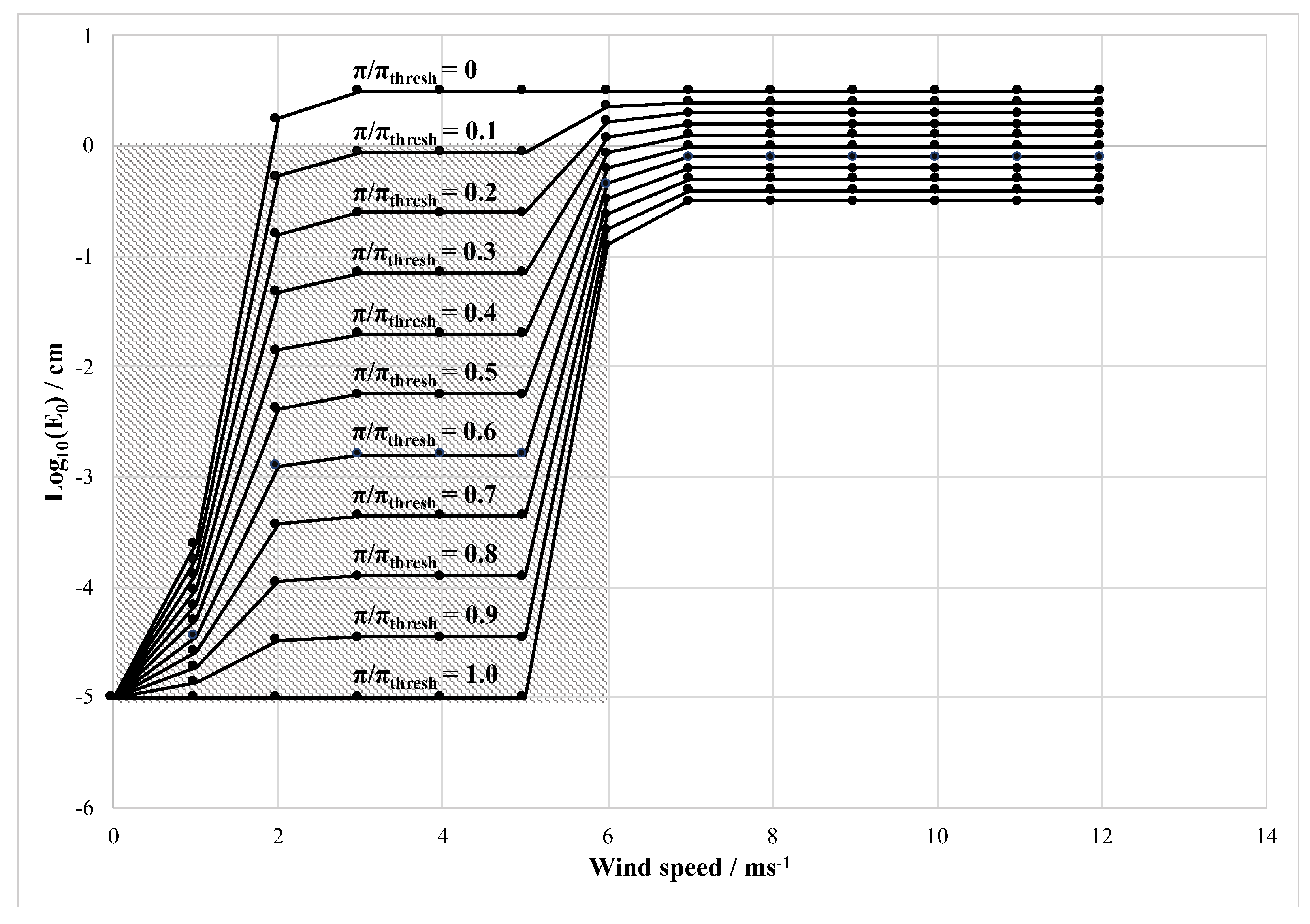
In addition to the macromolecules in the surface slick, capillary wave height is also dependent on wind velocity. In order to understand the dual impact of the surface pressure and the wind velocity on the capillary wave height, we represent the relationship visually (Figure 1) using the dynamics outlined in Equations (1) and (2). Assuming a surface pressure ratio (π/π_thresh) whose influence increases incrementally to reach a threshold value of 1.0 due to the presence of a surface slick and applying Equations (1) and (2), we show that while element height increases with increasing wind speed, the length is greatly reduced by increases in the surface pressure ratio (Figure 1). When slicking is introduced to varying degrees, the capillary wave height is demonstrably reduced for all wind speeds but has a maximal effect at intermediate velocities. At π/π_thresh = 0 there is the assumption of no surfactants to dampen the surface roughness, and thus the capillary wave height is only dependent on the wind speed. Conversely, at a π/π_thresh = 1, when the microlayer is assumed completely covered in surfactant, a minimum wind speed of 5 ms⁻¹ is required for the growth of any capillary waves. Figure 1 reflects the relationship between capillary wave height (E₀) vs. windspeed at π/π_thresh = 0 and unity, representing absent and maximal slick conditions, respectively initially developed by Barger (1970) [16]. However, here we have additionally shown how the relationship could change at intermediate π/π_thresh values. At π/π_thresh ≥ 0.1 and below a wind speed of about 6 ms⁻¹ the capillary wave height is < 1 cm. This portion of the parameter space readily generates capillary wave heights below the wavelengths relevant to microwave radar. We can therefore hypothesize a smooth reflective interfacial barrier under such conditions, with relatively high radar return. Capillary wave heights approach the centimeter scale when surface slicks are absent, thus falling within the altimetric diffuse reflection window (microwave frequency range). To zeroth order, we propose that scattering would be expected under these conditions.

2.3. Computing Surface Pressure for the North Atlantic from Lower Trophic Level Dynamics

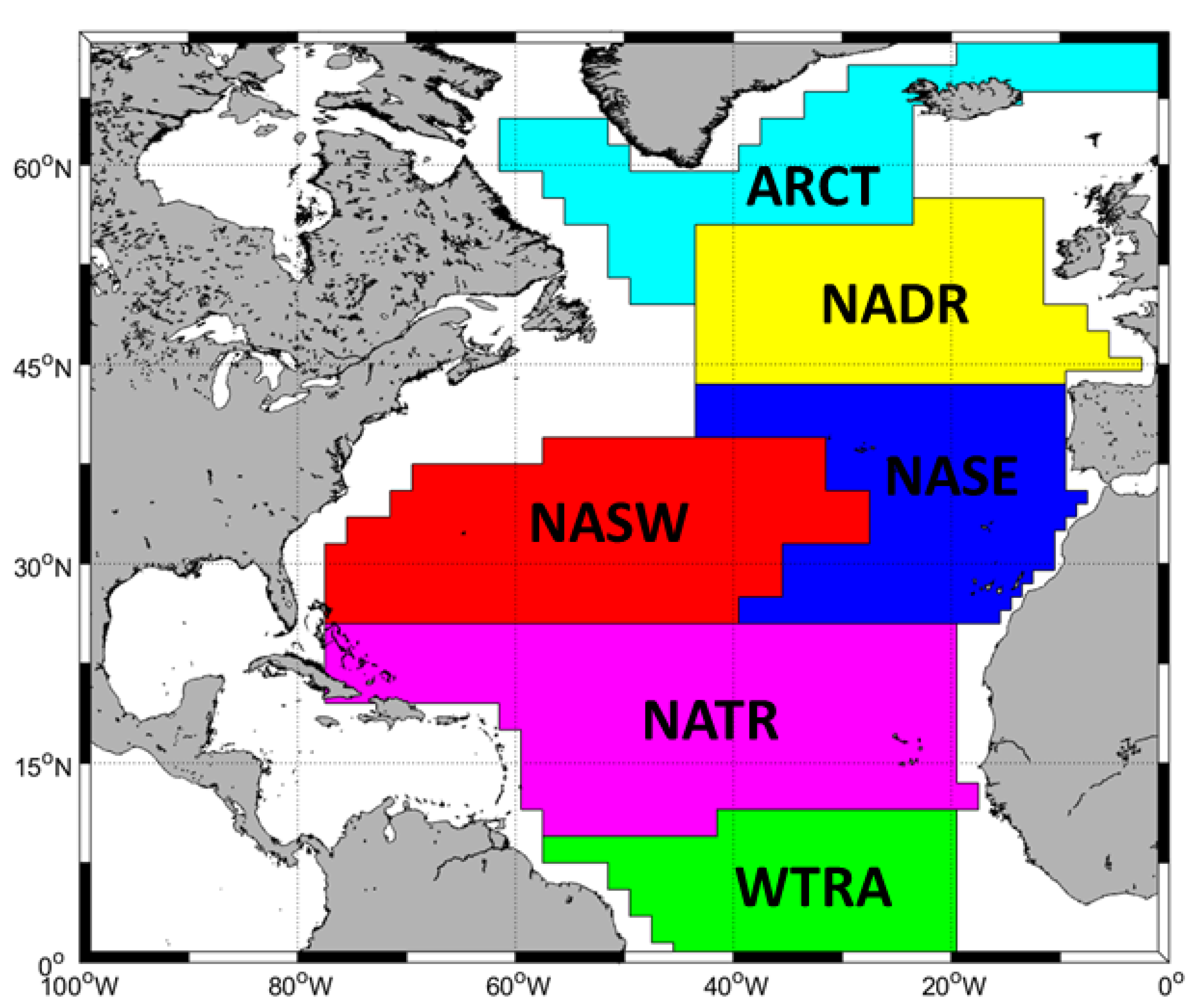
To demonstrate the utility of our reduced model approach in identifying Sigma-0 blooms in real world data, we apply it to satellite chl-a data for the North Atlantic region. Though marine organo-chemical measurement sets remain relatively rare, the North Atlantic is relatively data-rich, making this region a suitable area for our case study. The Northern Atlantic has been previously divided into sub-zones with distinct environmental and biogeochemical conditions (Figure 2, [19]), i.e., the Atlantic Arctic Province (ARCT), the North Atlantic Drift Province (NADR), the North Atlantic Subtropical Gyral Province East (NASE), the North Atlantic Subtropical Gyral Province West (NASW), the North Atlantic Tropical Gyral Province (NATR), and the Western Tropical Atlantic Province (WTRA). Applying our model to the observed chl-a concentration in each of these unique Longhurst sub-regions allows us to demonstrate how the surface pressure predictions will vary with environmental conditions (

Table 2. Computing surface pressure from chl-a in the North Atlantic ecological regions assuming a threshold surface pressure (π_thresh) of 3 mNm⁻¹.

Zone Longhurst	Summer Average chl-a (mgm−3)	Planktonic Carbon (Pc) (μM C)	[Protein] (Cprot) (μM C)	Protein Coverage Fraction (Θprot)	[Lipid] (Clip) (μM C)	Lipid Coverage Fraction (Θlip)	π (mNm−1)	π/πthreshold
ARCT	0.85	3.54	0.52	0.017	0.03	8.34 × 10−15	0.34	0.11
NADR	0.58	2.42	0.40	0.013	0.03	1.01 × 10−15	0.26	0.09
NASE	0.13	0.52	0.11	0.004	0.01	3.11 × 10−20	0.07	0.02
NATR	0.13	0.56	0.12	0.004	0.01	5.37 × 10−20	0.08	0.03
WTRA	0.20	0.85	0.17	0.006	0.01	1.08 × 10−18	0.11	0.04

).

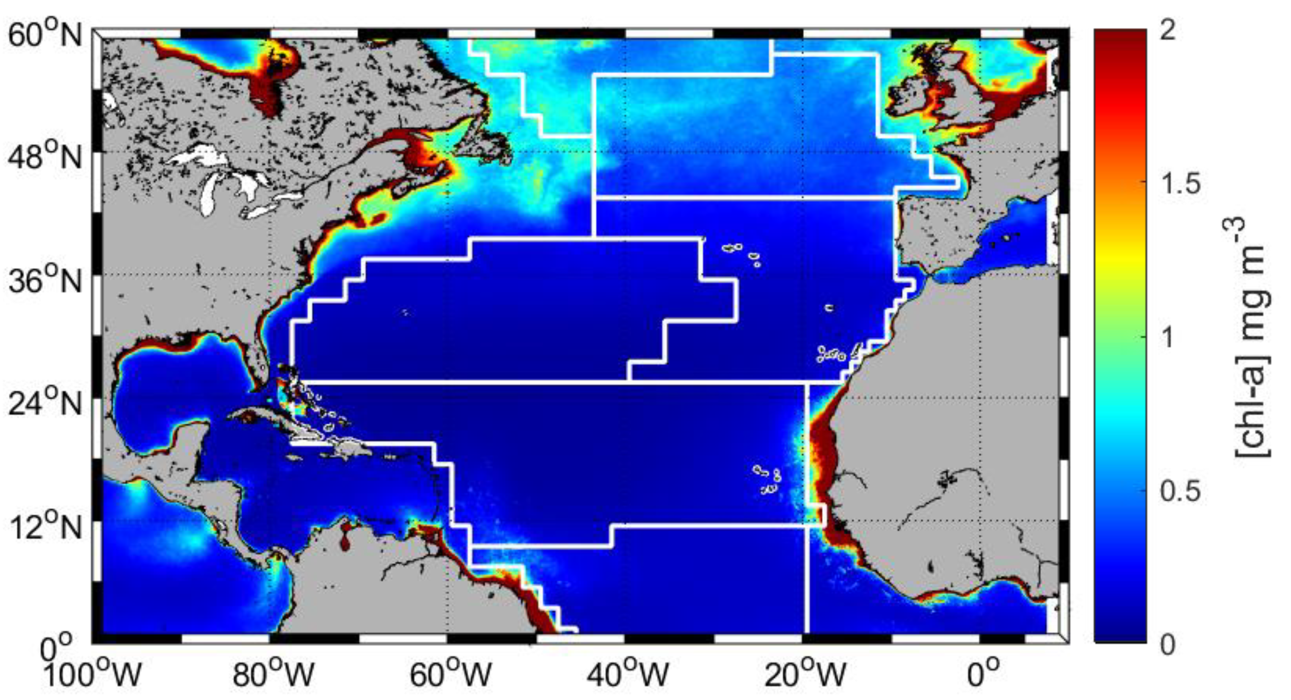
For each sub-zone in the North Atlantic (Figure 2), we extracted average summer (June/July/August) chl-a data from NASA Aqua Modis satellite observations for a fifteen-year period, (2002–2016).

Chlorophyll can be converted to phytoplanktonic carbon concentration (P_c), assuming a C: chl-a ratio of 50 mgC m⁻³:1 mgchl-a m⁻³ [20]. Standard macromolecular cytosol percentages (P_prot% = 0.6, P_lip% = 0.2, [12]) can then be applied to determine the fraction of the living carbon that is a cellular amphiphilic protein or lipid mass. The ecodynamic parameter values for g, K, Z, and γ can be approximate for each North Atlantic province, and they closely follow those used in the early but highly effective Fasham differential equations as described in Sarmiento et al. (1993) [15,21]. Surfactant lifetimes (τ_i) are assumed to depend on microbial and photochemical degradation and, along with the uncertainty factors (a_i), were taken from a global assessment of macromolecule surface activity [11].

Using model Equations (3)–(5), we computed surface pressure from our estimates of regional chl-a concentration, and by assuming a π threshold value of 3 mNm⁻¹, we computed the surface pressure ratios. We show that the higher the regional chl-a concentration, the greater the surface coverage by protein. Correspondingly, the surface pressure value and surface pressure ratio are similarly high. At 0.34 mNm⁻¹ the ARTC has the highest surface pressure value, whereas the NASE region has the lowest computed surface pressure value of 0.07 mNm⁻¹ (Table 2).

2.4. Spatial Variability of Roughness Length and Capillary Wave Height

As shown in Section 2.3, the combined effect of surface tension and wind speed determines the capillary wave height. Using the surface pressure values in each region of the North Atlantic (Figure 3,

Table 3. Roughness length and elemental height values calculated for each Longhurst region.

Zone Longhurst	Wind Speed (ms−1)	π/πthreshold	z0,surf (cm)	E0,surf (cm)
ARCT	2	0.11	0.04	0.45
NADR	2	0.09	0.06	0.61
NASE	2	0.02	0.13	1.33
NATR	6	0.03	0.29	2.91
WTRA	4	0.04	0.20	1.96

) along with the average summer wind speed values, we can compute the regional variation in the roughness length and the capillary wave height. By applying Equation (2) and our plot of elemental height vs. wind speed (Figure 1), the roughness length values are calculated for the relevant wind speed values (Table 3). The capillary wave heights can then be calculated using the direct proportionality shown in Equation (1).

Due to their differences in average wind and chl-a concentration, the North Atlantic regions have different capacities for capillary wave height. Increased capillary wave height values are achieved with low surface pressure and high wind speed values, and the low capillary wave height values are more likely at low wind speed and high surface pressure values. Although the highest surface pressure ratio value (0.11) was calculated in the ARCT region, the regionally averaged wind speed value is low (2 ms⁻¹), resulting in the lowest computed capillary wave height (0.45 cm). Conversely, even though a low surface pressure ratio (0.04) was in the WTRA region, the higher regionally averaged wind speed (4 ms⁻¹) led to a capillary wave height value of 1.96 cm. The NATR region has the highest reported wind speed values (6 ms⁻¹) with a low surface pressure ratio of 0.03, resulting the largest simulated capillary wave height of 2.91 cm.

2.5. Capillary Wave Height and Sigma-0 Frequency

The relationship between capillary wave height and the reflectivity of the surface is examined by plotting the fraction of a Longhurst region that has a Sigma-0 bloom occurrence at any point in the time series from 2001 to 2019 (Sigma-0 frequency, σ_f) against the calculated capillary wave height for each of the North Atlantic ecological regions considered. The annual average σ_f values (

Table 4. Annual and summer (June/July/August) Sigma-0 frequency values on a base ten logarithmic scale. Seasonal values are computed from these annual values based on seasonal TOPEX results shown in Mitchum et al. (2004) [3].

Zone Longhurst	Log10(σf)
	Annual	Seasonal
ARCT	−1.2	−0.72
NADR	−1.4	−0.92
NASE	−0.75	−0.27
NATR	−1.5	−1.5
WTRA	−0.8	−0.8

) were calculated by averaging estimates for σ_f from Jason 1, 2 and 3 satellite mission data for 2001–2019. We impose seasonality on the annual frequency with a scaling based on older (1992–1999) seasonal TOPEX/Poseidon data to synthesize the previously observed peaks and valleys in the data in summer and winter [3].

2.6. Sensitivity of Surfactant Concentration and Surface Pressure Threshold to Capillary Wave Height

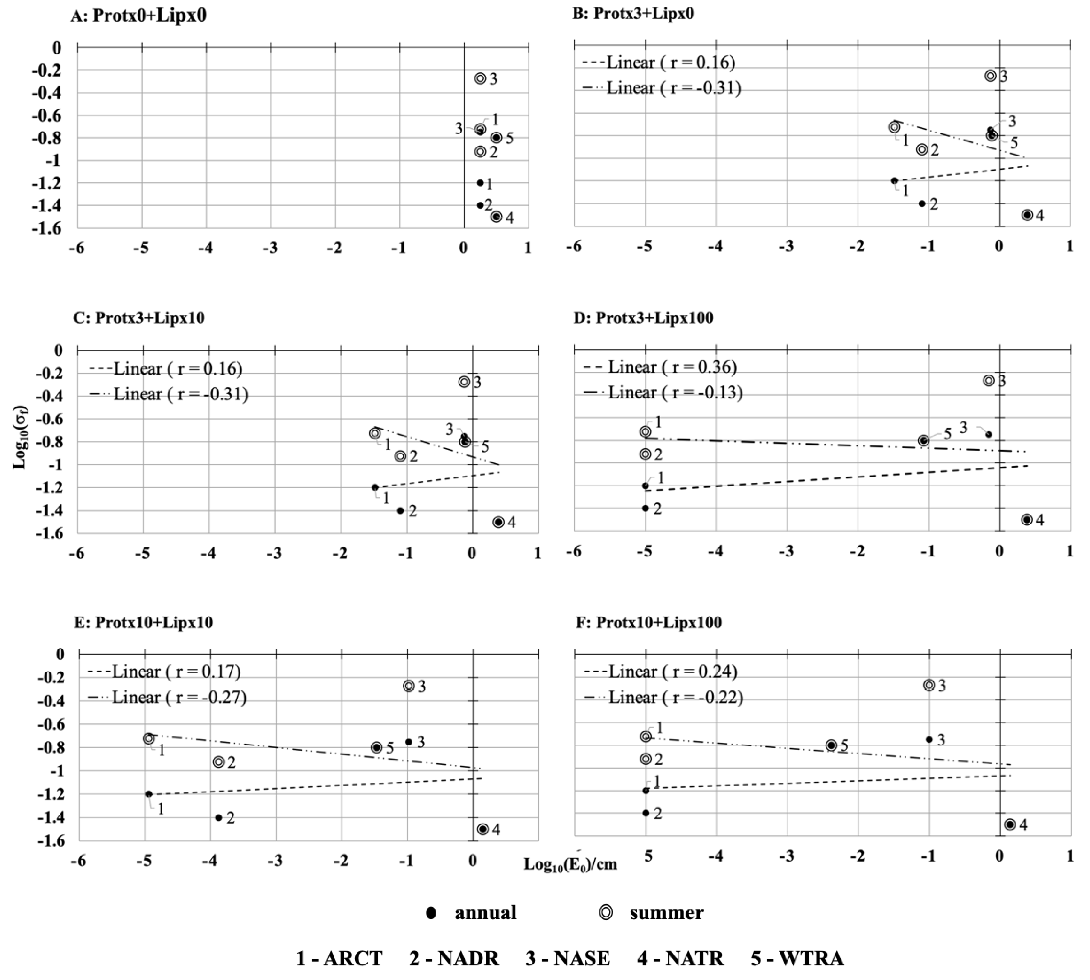
The sensitivity of our reduced model predicting the connection of sea-air interface reflectivity to Sigma-0 blooms was tested by varying the surfactant concentrations and the surface pressure threshold. Negative relationships were observed between the capillary wave height and Sigma-0 frequency (Figure 4 and Figure 5) indicating that the lower the wave height the higher Sigma-0 frequency.

To provide a reference framework and assist the reader in visualizing the potential for real-world correlations at the basin scale, we have plotted annual and seasonal Sigma-0 frequency against the capillary wave heights calculated in the absence of a surface slick (Figure 4A). This reference panel shows the distribution of friction-inducing wave heights for a pristine, abiotic ocean. No surfactant monolayer or film has been allowed and the Sigma-0 frequency values were permitted to range freely. Sigma-0 frequency values for the lower latitude WTRA and NATR regions were considered constant and a-seasonal because they lie along, or near, the equator where the solar angle and the biological activity in the upper water column can be assumed to be relatively constant [19]. Our other regions in the North Atlantic boast strong seasonal variability in both solar input and biological activity; as such, we computed both annual and summer Sigma-0 values for these regions.

2.7. Impact of Surfactant Concentration on Capillary Wave Heights

Our model results show that, in the absence of surfactants, there was no relationship between Sigma-0 frequency and capillary wave height (Figure 4A). When surfactant concentrations were increased, the capillary wave heights tended to be reduced, most notably in the ARCT and NADR regions due to the high surfactant concentration resultant by the high biological activity in those regions. Assuming the surfactants consisted solely of proteins (protx3), the summer Sigma-0 frequency negatively correlated (r = −0.31, Figure 4B) with the capillary wave height. In contrast, the annual Sigma-0 frequencies were weakly positively correlated (r = 0.16, Figure 4B), with the capillary wave height. Adding amphiphilic lipids to the surfactants with the primary multiplier of ten (to bring the concentration closely into an agreement with observations, Ogunro et al., 2015 [11]), did not notably change the relationship between the capillary wave height and the Sigma-0 frequency (r = −0.31, Figure 4C), indicating that lipid (×10) has only a small impact on the capillary wave height. At extreme lipid concentrations (×100 there was a weakly negative correlation between wave height and the Sigma-0 frequency (r = −0.13, Figure 4D), while on an annual basis the relationship was positive (r = 0.36, Figure 4D). Under such high lipid concentrations, the reduction in wave height in the ARCT and NADR regions is large relative to the other areas. Returning to a more moderate lipid concentration but increased protein concentration (×10) increased the relative strength of the negative correlation (r = −0. 27, Figure 4E), indicating surfactant behavior of proteins is high in diminishing the wave height, leading to a smooth surface which is more visible in the NASE region. Finally, with moderate protein but extreme lipid, the relative strength of the negative correlation was reduced only slightly (r = −0.22, Figure 4F), with respect to Figure 4E. The regions ARCT and NADR shift to the maximum wave height reduction, as the surface pressure reaches to its saturation point with the increased lipid concentration (Figure 4F) as these regions have the highest biological activity (ARCT = 0.85 mgm⁻³, NADR = 0.58 mgm⁻³). Additionally, the relative wave height reduction of the WTRA regions is considerable as it’s reported the third highest biological activity (0.20 mgm⁻³) in combination with the wind speed (4 ms⁻¹). The regions (ARCT, NADR and WTRA) with higher biological activity are more sensitive to wave height reduction.

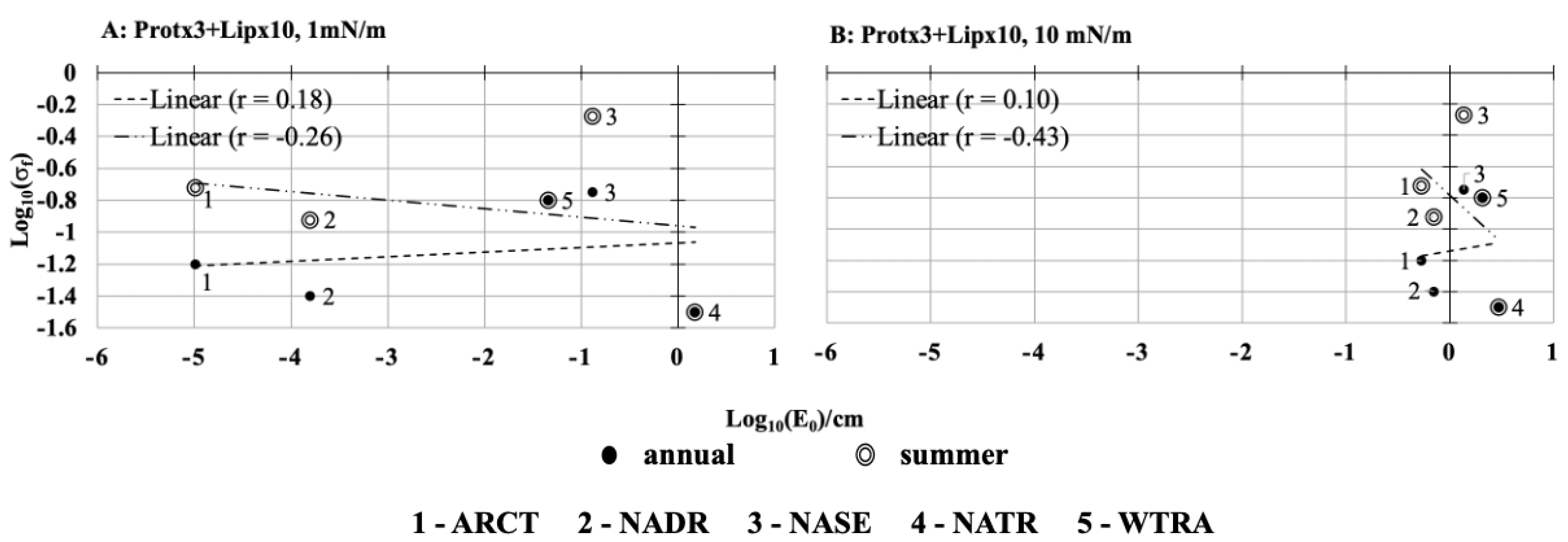
2.8. Impact of the Surface Pressure Threshold on Capillary Wave Height

The surface pressure threshold varies in a range based on the surfactant adsorption at the sea-air interface. For the surfactant concentration combination protein(×3) + lipid(×10), an additional series of sensitivity tests was carried out adjusting the surface pressure threshold value utilized in Equation (2) from the preliminary estimate of 3 mNm⁻¹, which is the maximum surface pressure value that exists in polar and coastal capillary waves seasonally [8,12], downward to 1 mNm⁻¹ to represents film pressure of natural sea water [22], and upward to 10 mNm⁻¹ to represent extreme surface pressure values [23]. The surface pressure threshold values could be changed based on a regions tendency to support slicks. The area and chemical composition of natural slicks are dependent on phytoplankton speciation, nutrient availability, and physical processes of the region. For the seasonal Sigma-0 frequency, negative correlations continue to exist with capillary wave height with both the reduced surface pressure threshold (r = −0.26, Figure 5A) and the increased surface pressure threshold (r = −0.43, Figure 5B). Conversely, the relationship between annual Sigma-0 frequencies and capillary wave height was weakly positively correlated with both low (r = 0.18, Figure 5A) and high (r = 0.10, Figure 5B) surface pressure thresholds. The damping of the capillary waves was more prominent at the 1 mNm⁻¹ surface pressure threshold as capillary wave heights were reduced to 1.0 × 10⁻⁵ (ARCT), 1.6 × 10⁻⁴ (NADR), 1.3 × 10⁻¹ (NASE), 1.5 (NATR), 4.5 × 10⁻² (WTRA) cm (summer, Figure 5A). In contrast, the capillary wave heights are relatively high 5.4 × 10⁻¹ (ARCT), 7.0 × 10⁻¹ (NADR), 1.4 (NASE), 2.9 (NATR), 2.0 (WTRA) cm when surface pressure threshold was increased to 10 mNm⁻¹ (summer, Figure 5B). A reduced pressure threshold is thus equivalent to the accumulation of several surfactants. Different region-wise changes to the capillary wave heights arose when implementing the different surface pressure thresholds of 1 mNm⁻¹ and 10 mNm⁻¹. With a reduced surface pressure, we find that the relative reduction in capillary wave height was ARCT > NADR > WTRA > NASE > NATR (Figure 5A) while with the increased surface pressure the change of the wave height was ARCT > NADR > NASE > WTRA > NATR (Figure 5B). In both instances, the regions where the highest chl-a concentrations were reported (ARCT, NADR, Table 2) were the regions where the capillary wave heights decreased more prominently. In the other regions (NASE, NATR and WTRA) both wind speed and surfactant concentration played a role in determining the resultant capillary wave height.

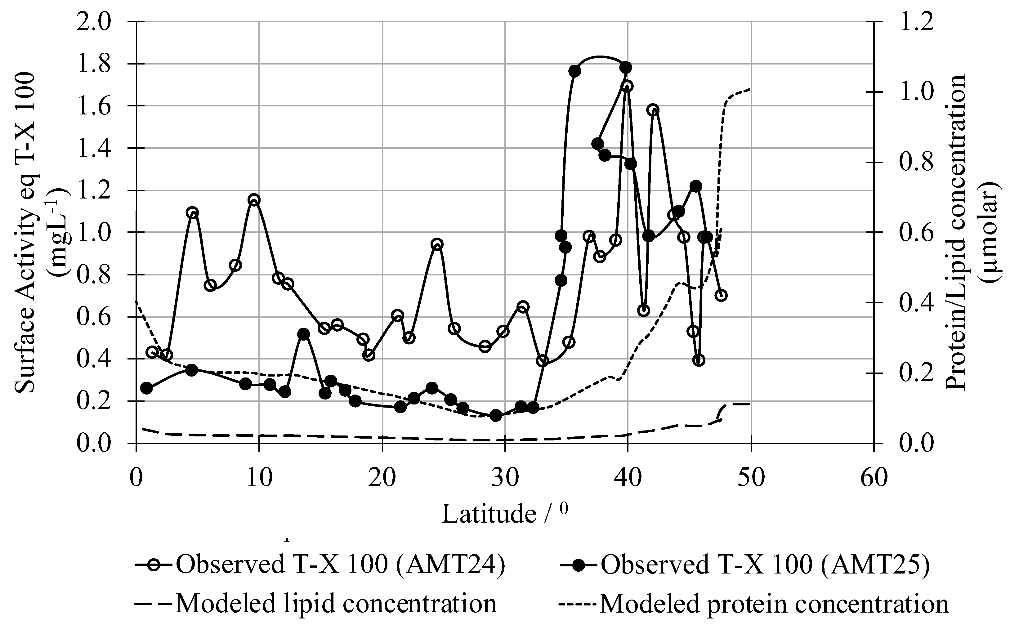
2.9. Regional Ship Track Comparisons

Observations of surface macromolecules are sparse, but one recent basin-scale field measurement dataset does focus specifically on surfactants within the open water microlayer. Using these observations, Sabbaghzadeh et al. (2017) [24] provided calibrated true ambient surface adsorption concentration (surface activity) for the entire Atlantic based on a well-known benchmark. We compare our surfactant concentrations determined from monthly averaged chl-a satellite observations extracted along the location of the ship track to their observed microlayer surfactant activity expressed as an equivalent adsorption effect of Triton-X-100(T-X-100)—a reference surfactant comprising a polyethylene oxide chain attached to an aromatic lipid. The surface adsorption concentration patterns along the two cruise tracks were markedly different (Figure 6), likely reflecting the different paths they took as they traversed the North Atlantic Ocean [24]. Between 10–30 °N the T-X-100 concentrations observed during the AMT25 cruise (~0.1–0.3 mgL⁻¹) were generally at least half the concentration observed at the same latitude on the later AMT24 cruise (~0.4–1.0 mgL⁻¹). The AMT24 cruise found increased concentrations between 5–10 °N that were not observed during AMT25. The concentration of T-X-100 on both cruises increased to a peak of ~1.7–1.8 mgL⁻¹ from 35–40 °N. Protein and lipid concentrations for the North Atlantic computed from satellite chl-a observations (Equation (5), Figure 3) broadly reproduce these observed patterns, with lower values below 35 °N. The modeled protein and lipid concentrations began to increase around 40 °N and were highest at 50 °N, the northernmost limit of the cruise track. The model also shows a dip-pattern from the maximum in equatorial waters (0–5 °N) falling to a minimum in the gyral regime (10–30 °N) and then rising again in the subtropics (30–50 °N) that is broadly consistent with observations.

3. Summary and Discussion

Ocean altimetric data are known to carry contamination due to the Sigma-0 bloom phenomenon, which leads to erroneous results in calculations of the sea surface height. Sigma-0 blooms (high backscattering values) are known to occur when the ocean surface is smooth and absent capillary waves [14,25]; usually in the presence of surface slicks and at low wind conditions [25,26]. However, to date, a valid qualitative or quantitative explanation for the blooms that connect the extent of surface slicking and wind speed to the capillary wave height, and thereby to the reflectivity of the sea-air interface, has not been provided. Here, a quantitative and qualitative biogeochemical approach was used to explain the origin of the surface slicks and how surfactant concentration could work with wind speed in determining capillary wave heights. Using a reduced bio-geo-chemical model we demonstrate that in the North Atlantic, regions of high biological activity and low wind speed will have capillary waves damped to heights less than typical radar altimeter wavelengths, resulting in a smooth sea-air interface with high radar backscattering values.

Our results suggest that the fraction of highly reflective ocean surface tends to increase as capillary wave amplitude decreases. We show that this is because as the capillary wave heights decrease the fraction of wave heights below the incident wavelength increases, which means that the sea-air interface presents as a smoother surface, and thus causes an increase in backscattering of a radar return signal. The amount of directional return depends on the roughness of the surface [2]). Radar altimeters transmit in the microwave region, i.e., at the centimeter scale. Capillarity of the global ocean interface takes the form of millimeter-centimeter scale objects, so the reflection versus scattering of an incoming radar signal will be highly dependent on damping [3,7]. This inverse relationship between reflectivity and wave heights is more obvious in low wind summertime conditions. During the summer, the biological activity and the injection of organic molecules are relatively high, which leads to a larger reduction of capillary wave height and, thus a smoother surface which is further facilitated by the low wind conditions. We can argue that an increase of the Sigma-0 bloom frequency caused by the biological activity would mean an increase in the backscattering value, i.e., the reflected power.

The increase in Sigma-0 frequency with the reduction in capillary wave heights depends on both the concentration of surfactant macromolecules, and on wind speed. The lysis of phytoplankton cells due to zooplankton grazing brings biomacromolecules to the surface ocean [9,13]. A fraction of these biomacromolecules contains chemical structures that tend to stay at the sea-air interface since the macromolecules contain both hydrophilic and hydrophobic parts. Adsorption of these macromolecules (mostly the lipids and proteins) coats at the sea-air interface with organic carbon chains and thereby changes the intermolecular interactions at the sea-air interface —readily depleting the micro-fastening system of the sea. We have demonstrated, with our modeled results, that in regions with lower regionally averaged wind speed (i.e., 2 ms⁻¹), (i.e., ARCT, NADR, and NASE), the surfactant concentration resulting from high biological activity will play a dominant role in damping the capillary wave height. Under low wind conditions the region (ARCT) that has the highest biological activity tends to have the lowest capillary wave height (0.45 cm). In contrast, the region with the lowest surfactant concentration (NASE) tends to have the highest capillary wave height (1.33 cm). Even though both NASE and NATR had relatively low biological activity, wave heights in the two regions were quite different. The capillary wave height increase in the WATR region was facilitated by the stronger regional wind speed (4 ms⁻¹). The combined effect of these biological and physical variables is also visible in the NATR region which has the highest regional wind speed (6 ms⁻¹). The relatively large capillary waves that one would expect were not observed. We argue that this is due to the surfactants from the moderate biological activity (indicated by the regional chl-a concentrations), damping the development of capillary waves.

Our study suggests that the impact of surfactants on capillary wave heights is sensitive to both the concentration and composition of surfactants. This sensitivity was demonstrated through the change to capillary wave height in response to changes in the surfactants. The relative heights of the capillary waves in each region shifted from ARCT < NADR < NASE < WTRA < NATR to ARCT < NADR < WTRA < NASE < NATR with the increase in the protein surfactant concentration by a factor of 10.

The adsorption isotherms for proteins and lipids are different due to their structural divergence. Under the same surface pressure condition and concentrations, lipids tend to adsorb more strongly onto the interface than the proteins. The adsorption process also depends on the concentrations of surface-active materials [27]. We assume that during the cell disruption the protein: lipid injection ratio would be 60%:20%. and protein had a longer lifetime (10 days) than the lipid (2 days). As such, modeled lipids concentrations were lower at the sea-air interface than proteins and the protein adsorption contributed more to the damping of capillary waves. If the lipid concentrations are same as proteins, the damping effect by lipids would be more prominent. The adsorption isotherm in the presence of both protein and lipid biomacromolecules is a combination of the individual protein and lipid isotherms, although the weight of the protein isotherm on the combined isotherms is relatively high.

Knowledge of biological distributions will allow the identification of regions where radar altimetry ocean reflection models should not assume a clean surface. Our research has provided evidence of the extent to which biological surface activity can impact the structure of the surface ocean. Consideration of this biological activity is critical when interpreting radar return signals from satellite altimeters used to map sea surface topography. By considering satellite derived chlorophyll concentration (our proxy for biological activity) and regional wind speed data our simple model provides estimates of expected capillary wave height and thereby predicts the potential for a reflective surface. Our model shows interconnected functionality between biological, chemical, and physical parameters for the capillary height damping calculations. Our simplified modeling approach could be used to identify the potential distribution of Sigma-0 bloom events. More extensive Sigma-0, chlorophyll, and wind speed data, ideally on a finer temporal and spatial scale, would be needed to further validate our predictions, and resolve the occurrence of Sigma-0 bloom and correct for them.

The relative impact of the surfactant concentration and surface pressure could be quantified by the relative reduction percentage [(E₀,_{no surfactant} − E₀,_{with surfactant})100/E₀,_{no surfactant}]. For regions with high biological activity (ARCT, NADR), the relative reduction percentage for all surfactant concentrations at 3 mN/m lies between 95.0–99.9%, indicating the damping is almost 100%. For low biological productivity regions NAST and NATR damping lie in the 59–95% and 21–54%, respectively. The larger ranges in these regions are due to variability in surfactant composition.

The drag coefficient is an important parameter in the transfer of wind momentum to the ocean [28], thus impacting the ocean circulation. As the magnitude of the drag partially depends on the height of the capillary waves, our research suggests that momentum flux in a region will be impacted by the presence of surface biology. The drag coefficient of the surface ocean has been previously speculated to have a dependency on the macromolecular carbon concentration [12]. Here, using our reduced model, we have reinforced this finding and demonstrated that the presence of surfactants at the sea-air interface could impact surface ocean roughness by as much as 21–99% in highly biologically active regions. To our knowledge, this link between biology, chemistry, and the physical domain is not currently represented in any Earth System Model and the drag coefficient is usually set to a constant value on the global scale. We argue that ignoring the impact of biological macromolecules on capillary wave height could result in understanding the drag coefficient and, thus, bias model estimates of ocean dynamics.

Several global marine biogeochemical models currently represent dissolved organic carbon, but only in a simple generic form [29,30]. We advocate an extension of this bio-chemical variable to explicitly represent the dominant macromolecules (proteins and lipids) such that a spatially explicitly biologically responsive drag coefficient can be computed. In our validation process, we observed that the surfactant adsorption data from two different cruise tracks did not closely resemble the calculated protein and lipid concentrations from our simple model. We speculate that this could be due to a miss-match in the timing of the satellite data which was a summer average (June–August) with the time of ship-board sampling (Sep–Oct). Furthermore, satellites are limited by optical depth so usually ‘see’ deeper (~5–10 m) than the very ocean surface. Nevertheless, our simple model was able to replicate the broad patterns and thus shows promise as a useful tool for altimetric data correction.

4. Concluding Remarks

In conclusion, radar reflectivity of the ocean surface depends on the damping of the capillary wave dimension, which we have shown is determined by both surfactant and wind speed. Because of the impact of surfactants on ocean roughness, and thus the drag coefficient, we believe biological surface activity should be considered when interpreting radar altimeter data.