Article

Decoupling of the Municipal Thermal Environment Using a Spatial Autoregressive Model

1
Bartlett School of Architecture, University College London, 22 Gordon St, London WC1H 0QB, UK
2
College of Architecture and Urban Planning, Tongji University, 1239 Siping Road, Shanghai 200092, China
3
Tongji Architectural Design (Group) Co., Ltd., 1230 Siping Road, Shanghai 200092, China
4
School of Architecture, The Chinese University of Hong Kong, 209, Lee Shau Kee Architecture Building, Shatin, N.T., Hong Kong
*
Author to whom correspondence should be addressed.
Atmosphere 2022, 13(12), 2059; https://doi.org/10.3390/atmos13122059
Submission received: 20 November 2022 / Revised: 3 December 2022 / Accepted: 5 December 2022 / Published: 8 December 2022

Abstract

:
In the rapid urbanization process, climate change has a huge impact on the urban thermal environment, and the urban heat island has attracted widespread attention from society. How to better detect, analyze, and evaluate the urban heat island effect has become a hot issue in current urban environmental research. However, the correlation analysis of heat island factors mostly adopts the conventional least square method, without considering the correlation of and the interaction between spatial elements. At the same time, the single analysis method makes it difficult to analyze environmental problems scientifically, which leads to great bias. Therefore, in this paper, the spatial autoregressive confusion model was used to analyze the satellite data of Beijing, and a preliminary temperature model of Beijing for all seasons was established. The regression results show that the surface temperature of Beijing has a strong spatial autocorrelation, and that the modified normalized difference water index and the normalized differential vegetation index have a strong negative effect on the land surface temperature. The prediction models established in this study can provide accurate and sustainable data support in the urbanization process and aid in the creation of a sustainable and effective urban environment.

1. Introduction

The development of cities is accompanied by the progress of human civilization, which is a very complex collection of human activities. According to the World Urbanization Prospects 2018, 55% of the world’s population was projected to live in cities by 2021. By 2050, 68% of the population will live in cities, and the global urban population will increase by 2.5 billion [1]. Nearly 90% of this growth has occurred in Asia and Africa. The density of buildings in cities is a key element in the process of the high-speed urbanization process. Green spaces are constantly changing into impermeable surfaces [2,3,4]. This will lead to the urban heat island (UHI) effect [5]. The worsening environmental effect leads to increased urban building energy consumption, decreased air quality [6], and damaged human health [7]. The construction of sustainable development is of great importance, so increasing attention is currently being paid to it, as can be seen by the establishment of the UNFCCC [8] and UN Climate Action Summit [9]. These conferences have provided a comprehensive discussion of temperature and sustainability and have contributed greatly to environmental sustainability efforts around the world.
UHI caused by urbanization not only increases the energy consumption of buildings in cities, but also brings largely hidden dangers to the health of urban residents [10]. Sachiko Kodera [11] conducted a computational study of three cities (Tokyo, Osaka, and Aichi) in Japan from 2013 to 2018, and the results of the study show that the incidence of disease in residents significantly increases after two or three consecutive hot weather events. Kai Chen’s [12] research found that a high temperature over four consecutive days will increase total mortality by 24.6%, cardiovascular mortality by 46.9%, respiratory mortality by 32.0% and stroke mortality by 51.3%. With the increase in urban temperature, morbidity and mortality related to heat waves are on the rise [13]. Therefore, it is very important to solve the problems of urbanization and the hidden dangers of high temperatures.
According to Tobler’s First Law of Geography, geographic phenomena exhibit strong spatial autocorrelations, and the heat island effect is no exception [14]. Therefore, some previous studies have elucidated the influence of each relevant index on heat islands, to some extent [15], but the spatial autocorrelation was not considered, which led to a low accuracy of the model. The emergence of various analytical tools, such as the spatial regression model, has led to a new perspective on spatial issues and is an important tool for studying urban phenomena. Therefore, in the method, we use a spatial regression model to solve these problems.

2. Study Area and Data

2.1. Study Scale

2.1.1. Spatial Scale

Beijing (east longitude 116°20′, north latitude 39°56′) is the capital of China. The climate of Beijing is a typical semi-humid continental monsoon climate in the north temperate zone. The total land area is 16,411 km 2 , of which the plain area is 6338 km 2 , accounting for 38.6%; and the mountainous area is 10,072 km 2 , accounting for 61.4%. Beijing includes many urban elements, such as residences, commerce, offices, parks, rivers, etc. Thus, the study results based on Beijing are universally applicable.

2.1.2. Spatial Scale

In this paper, we use remote sensing data from the NASA Landsat-8 satellite. The global cycle of the satellite is 16 days. The Landsat-8 satellite has two major sensors: the Operational Land Imager (OLI) and the Thermal Infrared Sensor (TIRS). The spatial resolution of nine multispectral bands of OLI is 30 m, and the spatial resolution of the two multispectral bands of TIRS is 120 m.
We should consider the influence of cloud amounts on land surface data through remote sensing image data inversion. Images with less than a 5% cloud amount should be selected. Because of the climate factors in Beijing, few satellite images meet the requirement for an accurate cloud amount inversion.
Thus, it is unrealistic to use bimonthly interval data [16]. To obtain more accurate results, we do not choose satellite data with the same quarterly time interval. The remote sensing image from midmonth is selected, according to the time characteristics of the four seasons in Beijing (01/2017, 05/2017, 07/2017, 09/2017) [16].

2.2. Urban Land Surface Characteristics

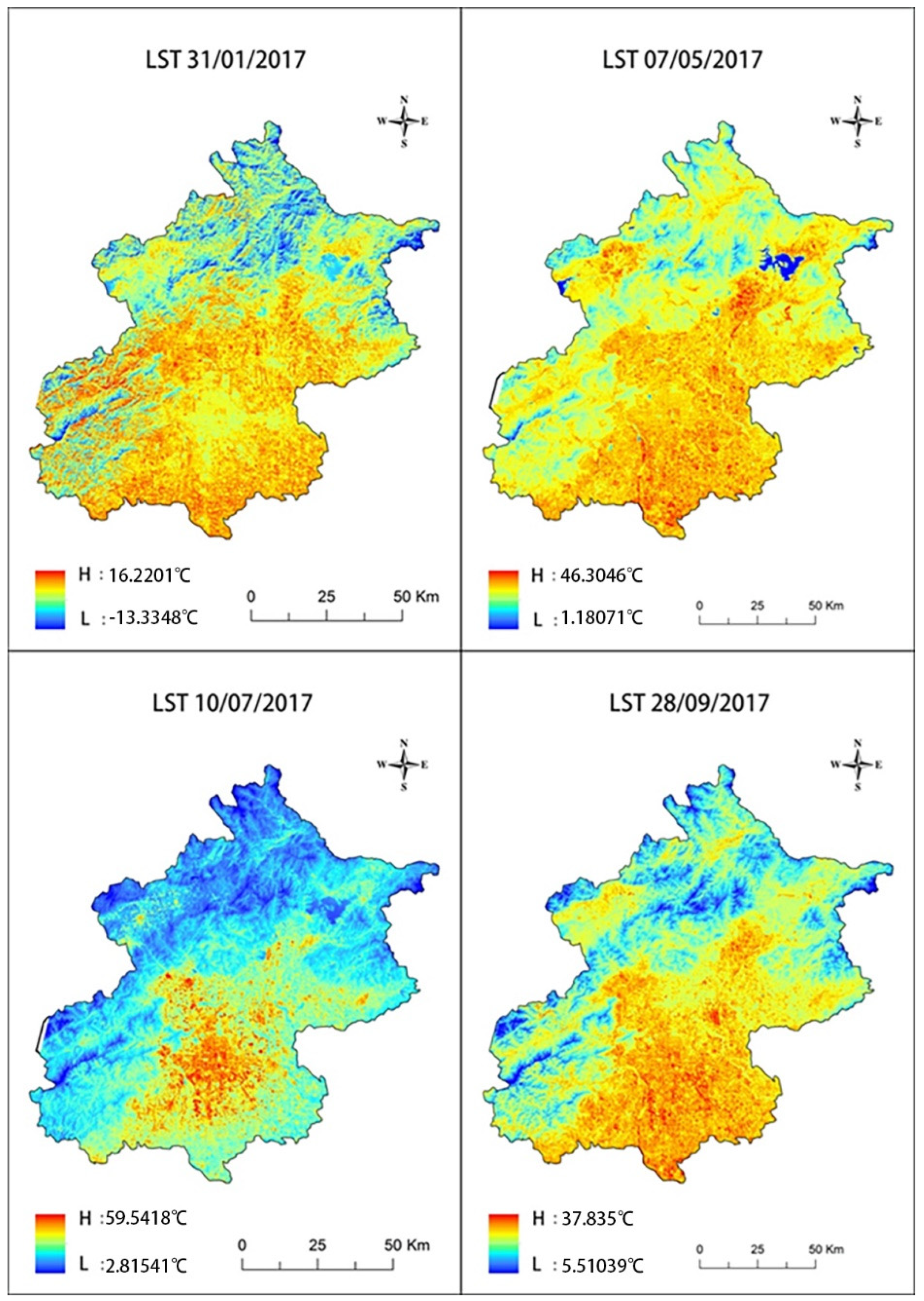
2.2.1. Land Surface Temperature (LST)

OLI bands from the NASA Landsat-8 satellite, with a spatial resolution of 30 m by 30 m, are used, but the spatial resolution of the TIRS bands is 120 m by 120 m. Therefore, the TIRS bands should be resampled to a resolution of 30 m by 30 m (a 120 m × 120 m unit will be divided into an average of 1630 m × 30 m units) for various unified spatial resolutions of the data (See Figure 1).
The spatial scale of the daily temperature (DT) of sparse weather stations in Beijing is not uniform, and the spatial resolution is too small, so it is not suitable to assess the spatial autocorrelation effect of air temperature [15]. The inversion of LST data by the atmospheric correction method has developed over many years [12], so obtaining the LST by this method is very accurate, and the LST has a higher spatial resolution. Thus, based on this method, we can study the effects between different city characteristics and LSTs across the whole city.

2.2.2. Normalized Differential Vegetation Index (NDVI)

Because the microclimate of the city can be improved by the cooling effect of vegetation transpiration and the canopy shading of hot sunlight radiation [17], the vegetation index has been used in many statistical studies. This index can be used to simply measure the coverage of plants. There are many different computing methods and different application scopes that can be used. The vegetation in Beijing is not dense, and the NDVI is suitable for use in areas with low vegetation density, so we chose to use the NDVI. The calculation is as follows:
NDVI = ρ NIR ρ RED ρ NIR + ρ RED
where ρ RED is the red band form Landsat-8; ρ NIR is the shortwave infrared band form Landsat-8. The NDVI ranged from −1.0 to 1.0. A value close to +1 indicates high-density vegetation, and a negative value indicates clouds, water, and snow (See Figure 2).
Due to the growth of vegetation, the NDVI will have a different performance over the course of one year. Therefore, the NDVI of the fourth phase of the year is computed through the ENVI (The Environment for Visualizing Images) platform.

2.2.3. Vegetation Classification (VC)

The vegetation classification (VC), based on vegetation coverage (VFC), can be roughly divided into 2 categories: remote sensing calculation methods and field survey methods. The field survey method is more accurate, but it is difficult to measure over a large area [18]. The remote sensing method is widely used to obtain the VFC within cities and is based on the NDVI. The calculation is as follows:
VFC = NDVI i NDVI min NDVI max NDVI min
where NDVI i is the NDVI value of point i; and NDVI min is the NDVI value of the bare soil, which should be close to 0 in theory, and NDVI max is the NDVI value of the densest vegetation in the dataset, which should be close to 1 in theory. According to the obtained VFC, vegetation is divided into four types, among which 0–0.3 represents no vegetation, 0.3–0.5 represents grassland, 0.5–0.7 represents shrubs, and 0.7–1.0 represents trees (see Figure 3).

2.2.4. Modified Normalized Difference Water Index (MNDWI)

Mcfeeters proposed the normalized difference water index (NDWI), but the water information based on NDWI is always intermingled with nonwater information, such as building information or vegetation information. Thus, the NDWI is not suitable to extract water data within the city. Xu proposed the modified normalized difference water index (MNDWI), which can be used to accurately extract water information data within vegetation areas and large cities [19]. The calculation is as follows:
MNDWI = ρ GREEN ρ MIR ρ GREEN + ρ MIR
MWI = W MNDVI = 0 ,    MNDWI < 0 1 ,    MNDWI 0
where   ρ GREEN is the green band form Landsat-8; ρ MIR is the middle infrared band form Landsat-8. When the MNDWI value is less than 0, the extracted water index (MWI) will be 0; if not, the MWI will be 1.

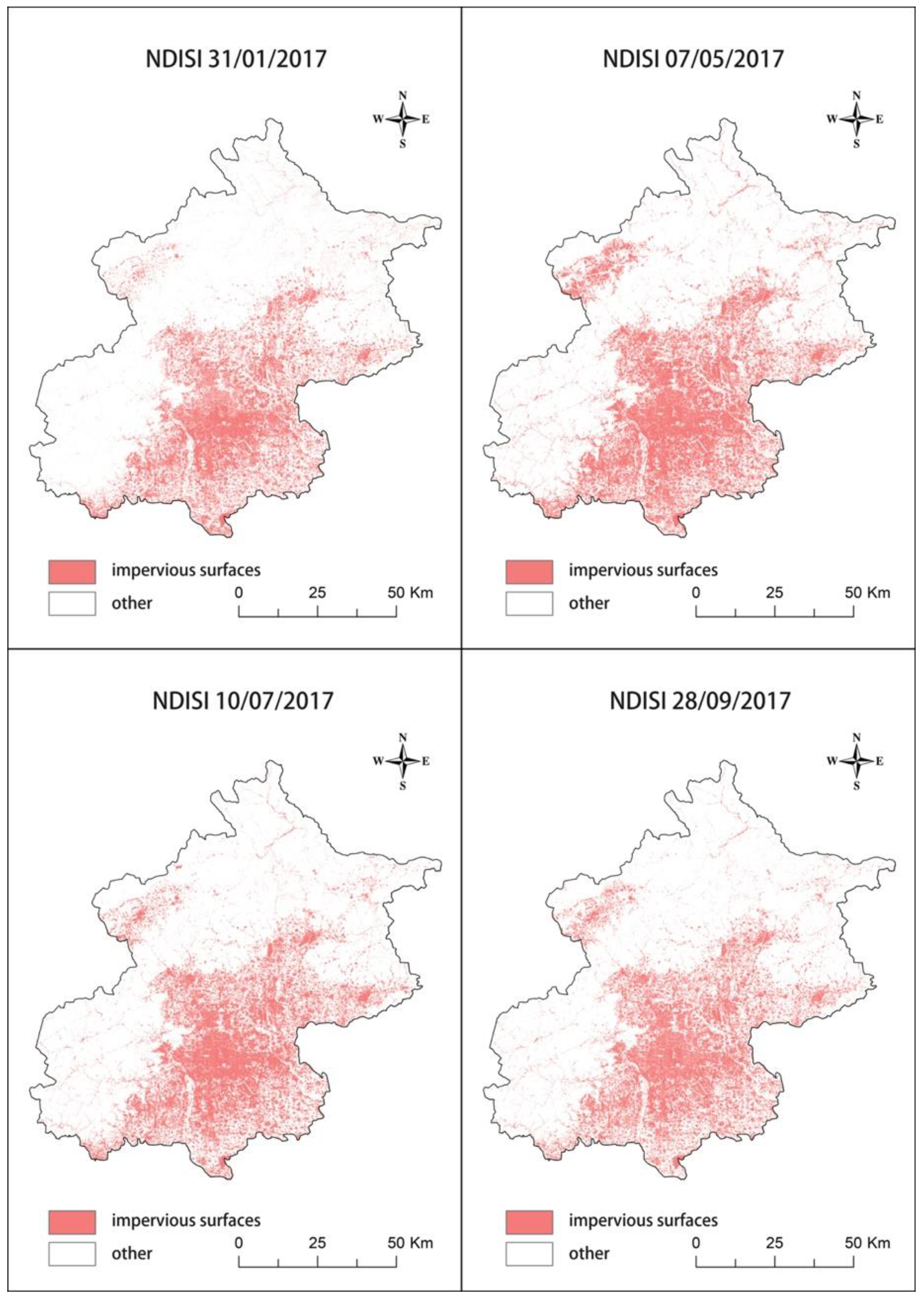
2.2.5. Impervious Surfaces Index (ISI)

The impervious surfaces of cities refer to surfaces covered by various building materials in urban areas. Xu proposed the normalized difference impervious surfaces index (NDISI) in 2008 [20]. It is an extracted impervious surface information method that excludes other surface elements in the city, such as soil, vegetation, and water. The calculation is as follows:
NDISI = ρ TIR MNDWI + ρ NIR + ρ MIR / 3 ρ TIR + MNDWI + ρ NIR + ρ MIR / 3
ISI = W NDISI     0 ,                             NDISI < 0.1028 1 ,               0.1028 NDISI 0.520     0 ,              0.520 < NDISI
where   ρ TIR is the thermal infrared band. When the NDISI value is less than 0.520 and greater than 0.1028, the ISI will output 1; if not, the ISI will output 0 (see Figure 4).

2.2.6. Building Silhouette Index (BS)

The normalized difference building index (NDBI), which is like the other various land surface indexes discussed in this article, is used by many researchers to obtain building information data in the study area [20,21]. This study focuses on the building greening social trend, which is advancing at a high speed, especially in the study area of Beijing, which has a positive greening policy. However, NDBI cannot distinguish high-vegetation buildings, and we did not choose this index to obtain building information data. We used the combination of BS and NDVI; buildings with high NDVI values are defined as “high-vegetation buildings;” thus, this method compensates for the drawback that high-vegetation buildings cannot be extracted correctly by remote sensing data. As mentioned above, we extract the building silhouette index (BS) from the accurate mapping data of the authoritative map provider GaoDe using ArcGIS software.

2.3. Social Economic Index

2.3.1. Population Density Index (PD)

We obtained PD data for every area in Beijing from the authoritative data provider Baidu. Based on the population data, we used inverse distance weighting (IDW) through ArcGIS software to obtain a population density index (PD) with a spatial resolution of 30 m [22,23].

2.3.2. NPP-VIIRS (NPP)g Silhouette Index (BS)

NPP-VIIRS (NPP) is the night light index from the Visible Infrared Imaging Radiometer Suite (VIIRS) of the NOAA National Center for Environment Information. The monthly average data used excluded lightning, moonlight, cloud cover, and other effects [24].

2.4. Data Extraction
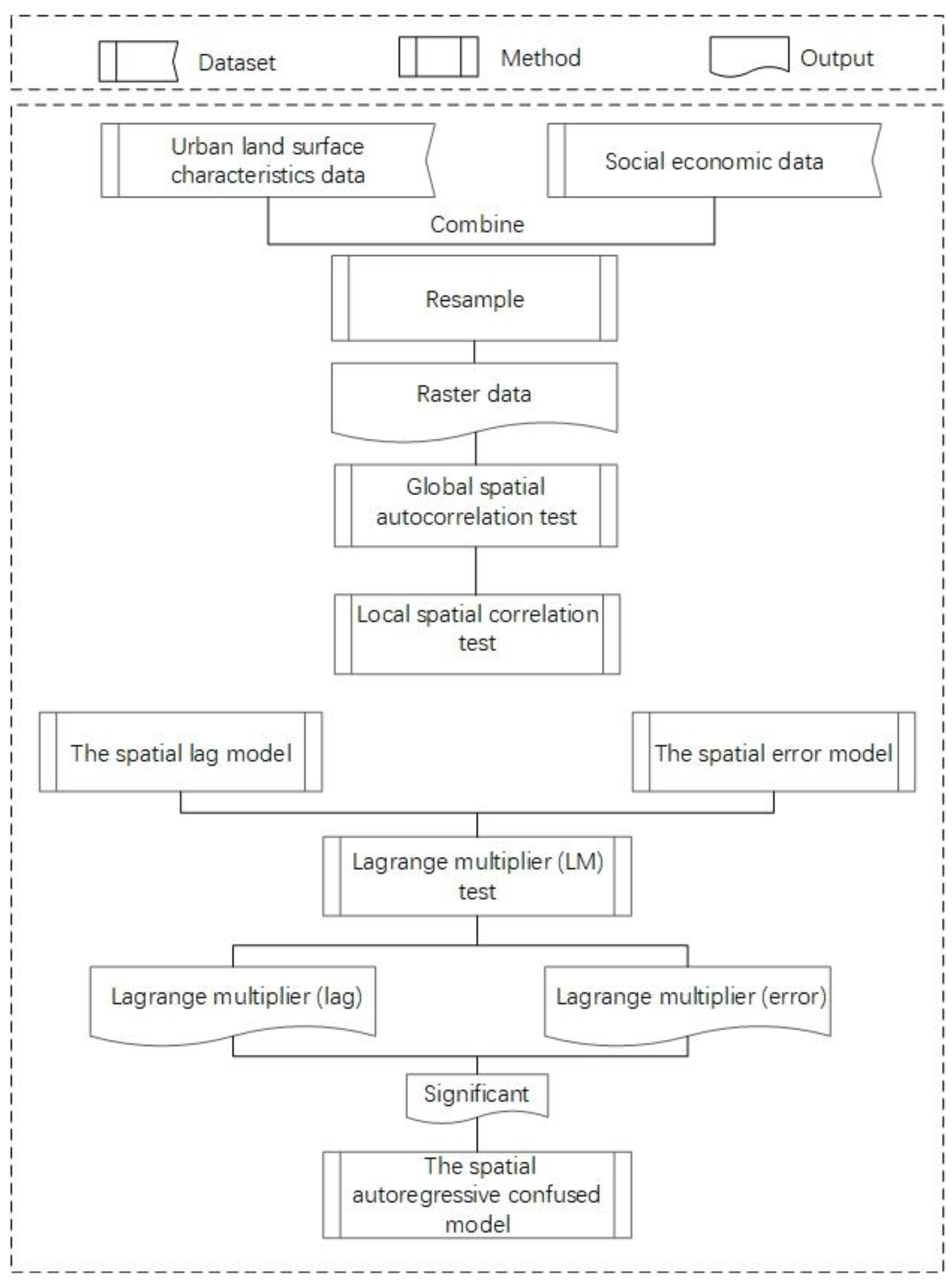
We matched the various rasterization urban land characteristic data obtained through remote sensing image data to the geographical coordinates of Beijing and built the netting twine, with an interval of 30 m. This formed 16,354 sample points that were evenly spatially distributed; among them, 37 points were excluded because of the effect of cloud cover. Finally, we obtained 16,312 sample points. There are characteristic data of eight types and four periods, used as the regression data, including LST, NDVI, VC, MWI, ISI, BS, PD, and NPP (see Table 1).

3. Methods

The 4-period LST image of Figure 1 shows that the LST has an apparent spatial clustering characteristic. This is because the mobility of air provides the possibility for changes in LST according to the surroundings.
In this study, urban land surface characteristics data and social-economic data are used to establish the prediction model of the urban heat island effect using a spatial autoregressive model, and the specific research steps are as follows (see Figure 5).

4. Experiment and Results

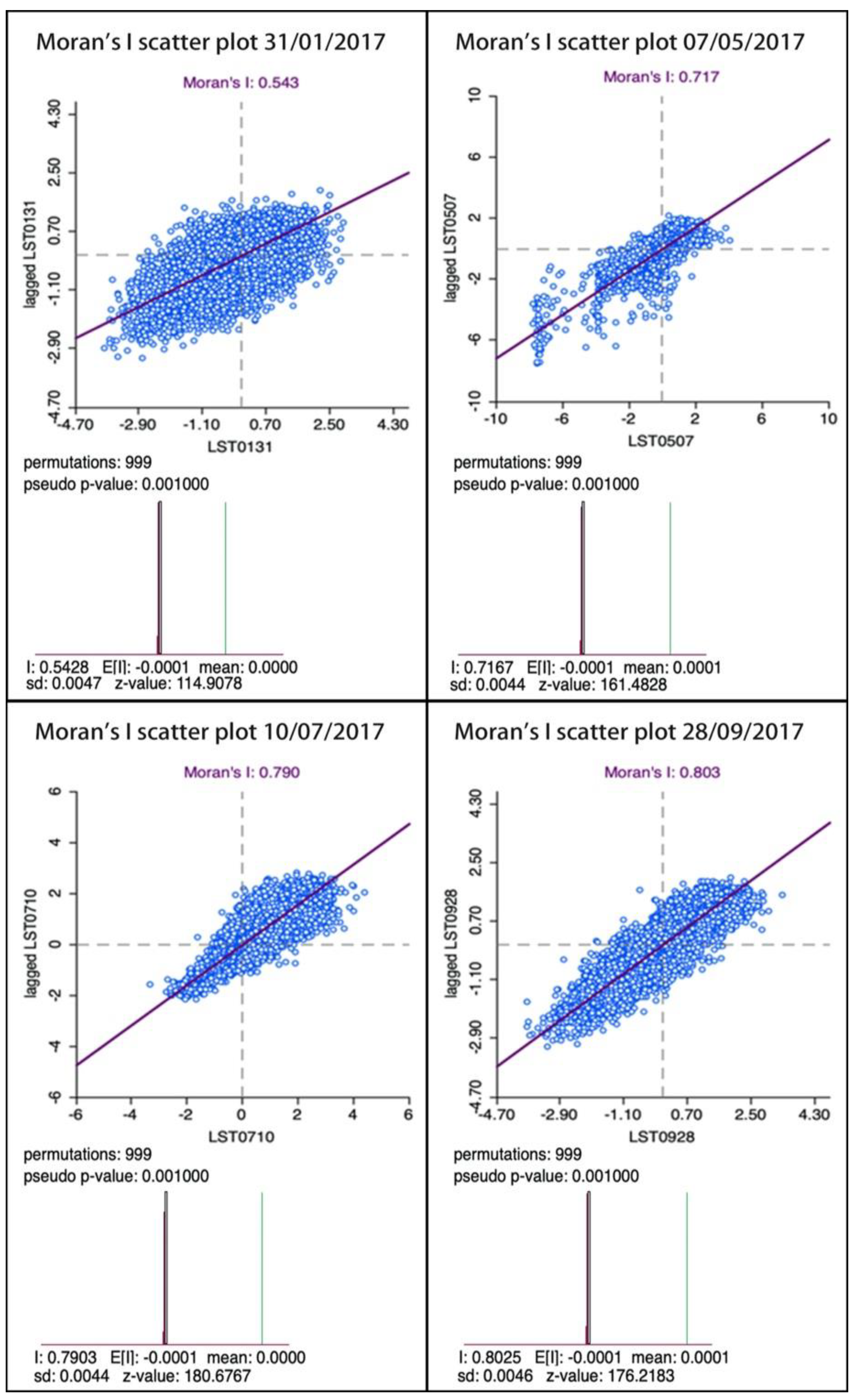
4.1. Global Spatial Autocorrelation Test

According to Tobler’s First Law of Geography, ‘Everything is related to everything else, but near things are more related to each other, the spatial autocorrelation test is the precondition in the spatial analysis. It is the correlation between measurement variables and the relationship between distant locations in geographical space. Global Moran’s I is an effective method for determining the spatial convergence of the described variables. The calculation is as follows:
I = n i = 1 n j = 1 n W ij X i X ¯ X j X ¯ i = 1 n j = 1 n W ij i = 1 n X i X ¯ 2
where n is the number of sample data, X i and X j are the observation values of spatial points i and j, and W ij is the spatial weight of spatial points i and j. The value range of Global Moran’s I is [−1, 1]. Value (0, 1] represents spatial clustering, value [−1, 0) represents spatial anomalies, and 0 means the data do not have a spatial autocorrelation.
The Moran’s values of the 4-period LST are all positive values, and the p-values are all less than 0.01 (see Figure 6). Thus, the results of the Global Moran’s tests have statistical significance. The spatial autocorrelation of the 10 July 2017 LST and 28 September 2017 LST is the most obvious, which is consistent with the LST prediction in the previous model estimation. In summary, the test results show that the 4 LST periods all have obvious global spatial autocorrelations. Therefore, the analysis of this dataset by the spatial regression model is reasonable.

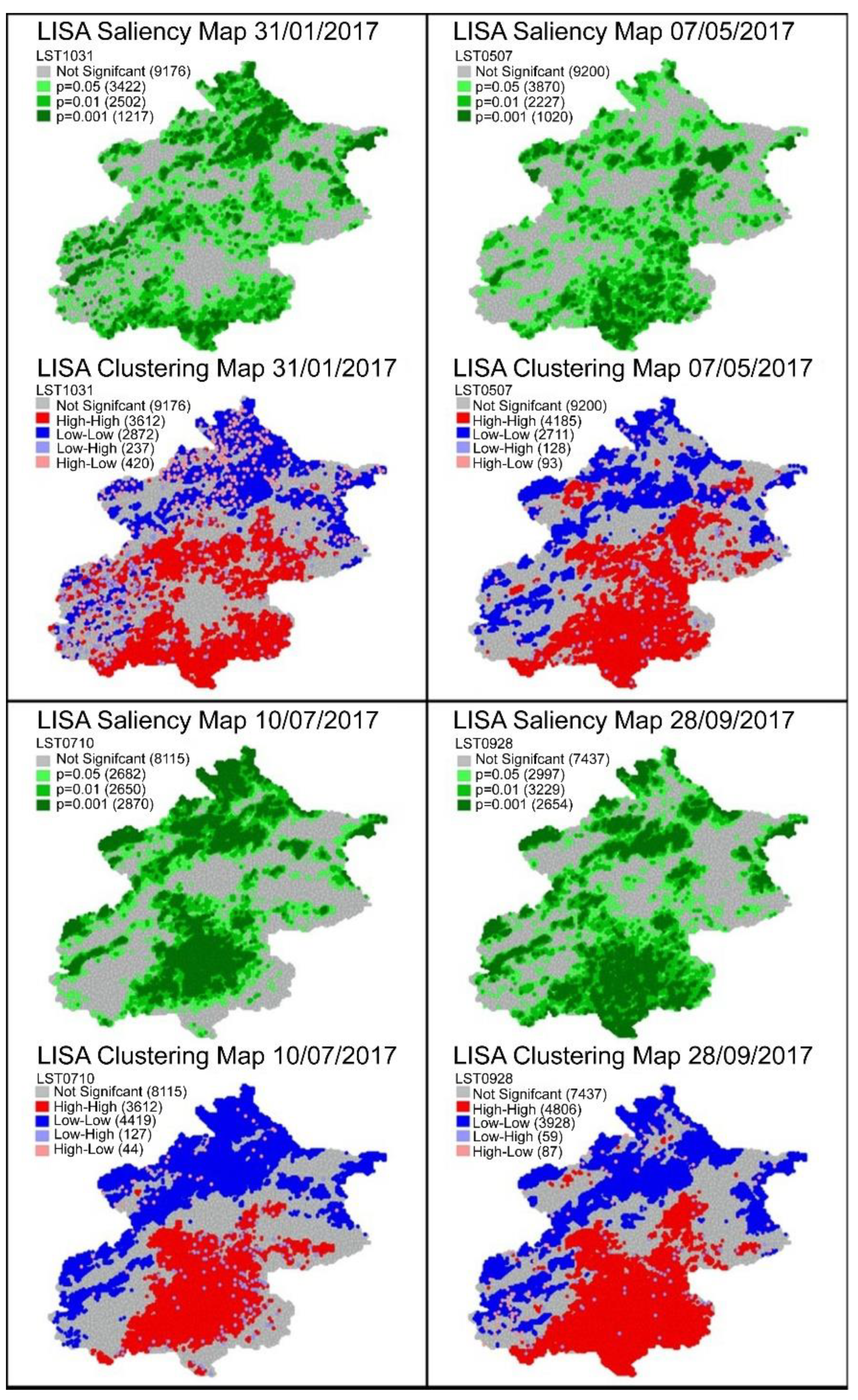
4.2. Local Spatial Correlation Test

The saliency of Beijing shows interesting changes with seasonal replacements (see Figure 7). Among them, in spring, summer, and autumn (7 May 2017, 10 July 2017, and 28 September 2017, respectively), the saliency of the urban area and mountain area is higher than that of the transition area. However, in winter (31 January 2017), the opposite is true. The saliency of its transition area is significantly higher than that of its urban and mountainous areas.
The LISA clustering map is composed of grey, red, blue, light blue, and light red colors, and these colors correspond to five different types of spatial correlations: nonsignificant, H-H, L-L, L-H, and H-l, respectively. In the map of the 4 LST periods, H-H and L-L account for a higher proportion (39.7%, 42.3%, 49.2%, and 53.5%), which shows that the spatial clustering of LST has a dominant position. Except for during winter, H-H is mainly distributed in urban areas, L-L is mainly distributed in mountainous areas, and L-H and H-L account for a small proportion (4%, 1.3%, 1%, and 0.8%). This result shows that the spatial anomalies of the data are low.
As mentioned above, the global and local spatial autocorrelations of all LST data have statistical significance. Thus, we should apply a spatial regression model to decrease the estimation bias caused by the OLS model, neglecting spatial correlation [25].

4.3. Classical Spatial Regression Model

The spatial regression model includes 2 kinds of classical regression models: the spatial lag model (SLM) and the spatial error model (SEM). SLM mainly considers the dependent variables of spatial autocorrelation, and SEM considers the errors of spatial autocorrelation [26]. The two models are as follows:
Spatial lag model (SLM)
LST = a 0 + ρ WLST + a 1 NDVI + a 2 VC + a 3 MWI + a 4 ISI + a 5 BS + a 6 PD + a 7 NPP + ε
In (8), ρ is the coefficient of spatial autocorrelation, a 0 is the model intercept, a 1 , a 2 ,…, a 7 are the deviation rate coefficients, ε is a random disturbance, and W is the spatial weight matrix, which represents the weight of the adjacent observations. The spatial weight matrix of this paper is constructed using the Queen connection, which means that if the sampling points i and j have the same edge or vertex, the element W ij is 1; otherwise, it is 0. SLM mainly considers the spatial correlation between the LST observed at sampling point i and the LST observed at neighboring sampling point j .
Spatial error model (SEM)
LST = a 0 + a 1 NDVI + a 2 VC + a 3 MWI + a 4 ISI + a 5 BS + a 6 PD + a 7 NPP + ε ε = λ W ε + μ  
In (9), λ is the error coefficient of spatial autocorrelation; μ is the error term. SEM mainly considers the spatial autocorrelation of error.

4.4. Spatial Regression Model Selection

To select from two kinds of classical spatial regression models, SLM and SEM were used for the calculation. We need to use the Lagrange Multiplier (LM) Test for the data, which contains two kinds of statistics: Lagrange Multiplier (lag) and Lagrange Multiplier (error). If the statistics of the LM (lag) are significant, SLM will be selected; otherwise, SEM will be selected. When the two kinds of statistics are both significant, we will use the robust LM test. This test also includes 2 kinds of statistics: robust LM (lag) and robust LM (error). If the statistics of robust LM (lag) are significant, SLM will be selected; otherwise, SEM will be selected [18].
Table 2 shows the results of LM and robust LM. We find that the probability of robust LM (error) value for the 31 January 2017 data is 0.00005, and although it is slightly higher than the robust LM (error) for the 31 January 2017 data, it still has high statistical significance. The other 14 kinds of statistics are all very significant. If we only choose SLM or SEM, a new estimation bias will result. Thus, we add the spatial autoregressive confused model (SAC). SAC considers the spatial autocorrelation of the dependent variable and error, and this is the combination between SLM and SEM. The SAC calculation is as follows:
LST = a 0 + ρ WLST + a 1 NDVI + a 2 VC + a 3 MWI + a 4 ISI + a 5 BS + a 6 PD + a 7 NPP + ε ε = λ W ε + μ  
To judge whether SAC is better than SLM, SEM, and OLS, we comparatively analyzed the R-squared value, as well as the log likelihood (LL), Akaike info criterion (AIC), and Schwarz criterion (SC). The larger the LL is, the smaller the AIC and SC will be, and the better the fitting effect of the model.
Table 3 shows the four kinds of statistics of OLS, SLM, SEM, and SAC. According to the value of R-squared, LL, AIC, and SC, we find that the evaluation of OLS is the lowest in the four regression models, and it has a large disparity with the others in various aspects. The result shows that the OLS has a significant estimation bias.
The statistics of SLM and SEM have their own advantages and disadvantages, but they are nearly the same. The result is the same as the significance comparison result of LM and Robust LM in the preceding paper, which shows that the OLS has obvious advantages because of SLM and SEM. Although they consider two types of aspects, dependent variable and error, these statistics have the same important meanings.
The evaluation of SAC is the best of the four regression models and has an obvious disparity with the other models. Although the R-squared of SAC is slightly smaller than that of the SEM in the 10 July 2017 data, the results of LL, AIC, and SC of SAC are better than those of SEM. The value range of R-squared is [0, 1], and it can only judge the fitting degree of the model and cannot judge whether the model has an overfitting problem. Therefore, we need to increase the consideration of LL, AIC, and SC to prevent the overfitting caused by the high accuracy of the model. In summary, the SAC model is selected for the spatial regression analysis.

4.5. SAC Analysis and Results

We use SAC to fit the regression curves between the eight independent variables and the dependent variable LST, and the fitting results of the four periods of data are shown in Table 4.
From the overall view of Table 4, the effects of NDVI and MWI on LST were very significant, and both were statistically significant. Among them, the standard coefficients of NDVI and MWI were negative in spring, summer, and autumn (−0.5030, −0.6143, and −0.3920 for NDVI; −0.8036, −0.5203, and −0.3920 for MWI), indicating that NDVI and MWI have a strong cooling effect on the temperature of the city. Therefore, increasing the two variables, NDVI and MWI, can effectively mitigate the UHI.
Specifically, among all variables, the highest standard coefficient is MWI in the spring model, which indicates that the influence of water bodies shows a large variation, with a standard coefficient of −0.8036, thus showing that MWI can significantly decrease the LST in spring, and when other conditions are constant, an increase of 0.1 in MWI will reduce the LST by 0.8697 °C. This is because the effect of water bodies on urban temperature lies in their conversion of sensible and latent heat fluxes. On the one hand, the high heat capacity creates a “thermostat effect” on the water body, compared to the surrounding building materials [27]. On the other hand, evaporation from water bodies leads to a significant “oasis effect,” a phenomenon that plays an important role in reducing the surrounding surface temperature [28]. Water bodies act as cooling islands (UCI) in urban areas due to the temperature difference in the nearby environment [29]. Therefore, the urban water space is a key point to mitigate the heat island effect.
Secondly, the effect of NDVI showed a large variation among all variables, which indicates that NDVI can significantly improve LST. In spring, when NDVI increases by 0.1, LST will decrease by 0.4380 °C; in summer, when NDVI increases by 0.1, LST will decrease by 0.5133 °C; in autumn, when NDVI increases by 0.1, LST will decrease by 0.4196 °C; interestingly, in the winter model, the coefficient of NDVI was positive, indicating a negative correlation between LST and NDVI in winter, which was not the same as initially expected. This is because the leaves of vegetation may have the function of blocking the wind, thus reducing the influence of cold winter air. NDVI not only reduces LST, but also improves winter temperatures. In general, the greater the NDVI, the lower the surface temperature, which indicates that increasing the urban greening rate has a mitigating effect on the urban heat island and can have a cooling effect. Greening can reduce the outdoor temperature of buildings through the evaporative effect of plants and the blockage of sunlight by vegetation [30]. The convergence of urban green spaces, such as urban parks and public facilities, can change the urban microenvironment by affecting the local temperature, humidity, and air composition to obtain a relatively cooler area.
Finally, the standard coefficients of ISI and BS are significantly different from NDVI and MWI, and the coefficients of BS in spring and winter and ISI in spring and autumn are both negative. Thus, buildings in the city are not a significant cause of UHI, but buildings encroach on vegetation space, leading to higher temperatures.

5. Conclusions

Previous studies have mostly focused on a single spatial scale and used classical statistical analysis as the calculation method, which cannot realize the consideration of spatial effects. Moreover, it is difficult to consider the influence of the plastic area unit problem on the analysis results, and the results often have large errors. The above problems motivated this study to investigate the spatial relationship between heat island intensity and surface environment using a spatial regression confusion model.
Firstly, eight surface environmental and socioeconomic data, including LST, NDVI, VC, MWI, ISI, BS, PD, and NPP, were obtained using the NASALandsat-8 satellite and authoritative data from the Beijing Meteorological Station. To evaluate the heat island effect in different periods throughout the year, we obtained four datasets for different time periods.
Then, we checked the spatial correlation of the datasets and evaluated the data of seven independent variables for each dataset using the SAC model to establish the relationship between the above data and surface temperature. The regression results show that the surface temperature in Beijing has a strong spatial autocorrelation, in which NDVI and MWI have a strong influence on the outdoor temperature of buildings at different times of the year, indicating that water bodies and greenery are the main factors determining the surface temperature in the city.
Therefore, in the urbanization process of addressing climate change, it is necessary to increase urban greening and protect water bodies to mitigate the urban heat island effect and promote ecological city construction. Specifically, over the course of a year, when the NDVI increases by 0.1, the LST will decrease by a maximum of 0.803 °C. When the MWI increases by 0.1, the LST decreases by 0.392 °C to 0.503 °C. This conclusion provides policymakers with a valid judgment criterion that can be used for targeted policy formulation and sustainable urban planning.

Author Contributions

Conceptualization, Z.W. and Q.J.; methodology, Q.J.; software, Q.J.; validation, Z.W., Q.J. and X.L.; formal analysis, Q.J.; investigation, Q.J.; resources, Q.J. and X.L.; data curation, Q.J.; writing—original draft preparation, X.L. and Q.J.; writing—review and editing, Q.J. and J.D.; visualization, Q.J. and Y.W.; supervision, Z.W. and Q.J.; project administration, Z.W. and Q.J.; funding acquisition, Z.W. and Q.J. All authors have read and agreed to the published version of the manuscript.

Funding

This research was funded by The International Knowledge Center for Engineering Sciences and Technology (IKCEST) under the auspices of UNESCO, Beijing 100088, China.

Institutional Review Board Statement

Not applicable.

Informed Consent Statement

Informed consent was obtained from all subjects involved in the study.

Data Availability Statement

Not applicable.

Conflicts of Interest

The authors declare no conflict of interest.

References

  1. World Urbanization Prospects—Population Division—United Nations. Available online: https://population.un.org/wup/ (accessed on 1 December 2022).
  2. Wu, Z.; Qiao, R.; Zhao, S.; Liu, X.; Gao, S.; Liu, Z.; Ao, X.; Zhou, S.; Wang, Z.; Jiang, Q. Nonlinear Forces in Urban Thermal Environment Using Bayesian Optimization-Based Ensemble Learning. Sci. Total Environ. 2022, 838, 156348. [Google Scholar] [CrossRef]
  3. Shen, X.; Chen, M.; Ge, M.; Padua, M.G. Examining the Conceptual Model of Potential Urban Development Patch (PUDP), VOCs, and Food Culture in Urban Ecology: A Case in Chengdu, China. Atmosphere 2022, 13, 1369. [Google Scholar] [CrossRef]
  4. Huang, C.; Zhang, G.; Yao, J.; Wang, X.; Calautit, J.K.; Zhao, C.; An, N.; Peng, X. Accelerated Environmental Performance-Driven Urban Design with Generative Adversarial Network. Build. Environ. 2022, 224, 109575. [Google Scholar] [CrossRef]
  5. Yu, Z.; Yao, Y.; Yang, G.; Wang, X.; Vejre, H. Spatiotemporal Patterns and Characteristics of Remotely Sensed Region Heat Islands during the Rapid Urbanization (1995–2015) of Southern China. Sci. Total Environ. 2019, 674, 242–254. [Google Scholar] [CrossRef] [PubMed]
  6. Song, Y.; Zhang, B. Using Social Media Data in Understanding Site-Scale Landscape Architecture Design: Taking Seattle Freeway Park as an Example. Landsc. Res. 2020, 45, 627–648. [Google Scholar] [CrossRef]
  7. Akbari, H.; Kolokotsa, D. Three Decades of Urban Heat Islands and Mitigation Technologies Research. Energy Build. 2016, 133, 834–842. [Google Scholar] [CrossRef]
  8. The Paris Agreement|UNFCCC. Available online: https://unfccc.int/process-and-meetings/the-paris-agreement/the-paris-agreement (accessed on 31 October 2022).
  9. UN Climate Action Summit 2019|United Nations Development Programme. Available online: https://www.undp.org/ukraine/news/un-climate-action-summit-2019?utm_source=EN&utm_medium=GSR&utm_content=US_UNDP_PaidSearch_Brand_English&utm_campaign=CENTRAL&c_src=CENTRAL&c_src2=GSR&gclid=Cj0KCQjwwfiaBhC7ARIsAGvcPe6uWw0qrDrhpP_cmxVjQWJt5K6h_M1IISCc8TXQwiA3lYUUaW3evgoaArLcEALw_wcB (accessed on 31 October 2022).
  10. Silveira, I.H.; Oliveira, B.F.A.; Cortes, T.R.; Junger, W.L. The Effect of Ambient Temperature on Cardiovascular Mortality in 27 Brazilian Cities. Sci. Total Environ. 2019, 691, 996–1004. [Google Scholar] [CrossRef]
  11. Kodera, S.; Nishimura, T.; Rashed, E.A.; Hasegawa, K.; Takeuchi, I.; Egawa, R.; Hirata, A. Estimation of Heat-Related Morbidity from Weather Data: A Computational Study in Three Prefectures of Japan over 2013–2018. Environ. Int. 2019, 130, 104907. [Google Scholar] [CrossRef]
  12. Chen, K.; Bi, J.; Chen, J.; Chen, X.; Huang, L.; Zhou, L. Influence of Heat Wave Definitions to the Added Effect of Heat Waves on Daily Mortality in Nanjing, China. Sci. Total Environ. 2015, 506–507, 18–25. [Google Scholar] [CrossRef]
  13. Vicedo-Cabrera, A.M.; Sera, F.; Guo, Y.; Chung, Y.; Arbuthnott, K.; Tong, S.; Tobias, A.; Lavigne, E.; de Sousa Zanotti Stagliorio Coelho, M.; Hilario Nascimento Saldiva, P.; et al. A Multi-Country Analysis on Potential Adaptive Mechanisms to Cold and Heat in a Changing Climate. Environ. Int. 2018, 111, 239–246. [Google Scholar] [CrossRef]
  14. Waters, N. Tobler’s First Law of Geography. In International Encyclopedia of Geography: People, the Earth, Environment and Technology; Richardson, D., Castree, N., Goodchild, M.F., Kobayashi, A., Liu, W., Marston, R.A., Eds.; John Wiley & Sons, Ltd.: Oxford, UK, 2017; pp. 1–13. ISBN 978-0-470-65963-2. [Google Scholar]
  15. Luo, Z.; Sun, C.; Dong, Q.; Qi, X. Key Control Variables Affecting Interior Visual Comfort for Automated Louver Control in Open-Plan Office—A Study Using Machine Learning. Build. Environ. 2022, 207, 108565. [Google Scholar] [CrossRef]
  16. Chun, B.; Guldmann, J.-M. Impact of Greening on the Urban Heat Island: Seasonal Variations and Mitigation Strategies. Comput. Environ. Urban Syst. 2018, 71, 165–176. [Google Scholar] [CrossRef]
  17. Qiao, Z.; Tian, G.; Xiao, L. Diurnal and Seasonal Impacts of Urbanization on the Urban Thermal Environment: A Case Study of Beijing Using MODIS Data. ISPRS J. Photogramm. Remote Sens. 2013, 85, 93–101. [Google Scholar] [CrossRef]
  18. Zhang, W.; Yang, X.; Manlike, A.; Jin, Y.; Zheng, F.; Guo, J.; Shen, G.; Zhang, Y.; Xu, B. Comparative Study of Remote Sensing Estimation Methods for Grassland Fractional Vegetation Coverage—A Grassland Case Study Performed in Ili Prefecture, Xinjiang, China. Int. J. Remote Sens. 2019, 40, 2243–2258. [Google Scholar] [CrossRef]
  19. Xu, H. A New Index for Delineating Built-up Land Features in Satellite Imagery. Int. J. Remote Sens. 2008, 29, 4269–4276. [Google Scholar] [CrossRef]
  20. Correia Filho, W.L.F.; de Barros Santiago, D.; de Oliveira-Júnior, J.F.; da Silva Junior, C.A. Impact of Urban Decadal Advance on Land Use and Land Cover and Surface Temperature in the City of Maceió, Brazil. Land Use Policy 2019, 87, 104026. [Google Scholar] [CrossRef]
  21. Guha, S.; Govil, H.; Dey, A.; Gill, N. Analytical Study of Land Surface Temperature with NDVI and NDBI Using Landsat 8 OLI and TIRS Data in Florence and Naples City, Italy. Eur. J. Remote Sens. 2018, 51, 667–678. [Google Scholar] [CrossRef] [Green Version]
  22. Ghaedrahmati, S.; Alian, M. Health Risk Assessment of Relationship between Air Pollutants’ Density and Population Density in Tehran, Iran. Hum. Ecol. Risk Assess. Int. J. 2019, 25, 1853–1869. [Google Scholar] [CrossRef]
  23. Godin, F.; Degrave, J.; Dambre, J.; De Neve, W. Dual Rectified Linear Units (DReLUs): A Replacement for Tanh Activation Functions in Quasi-Recurrent Neural Networks. Pattern Recognit. Lett. 2018, 116, 8–14. [Google Scholar] [CrossRef] [Green Version]
  24. Gao, N.; Li, F.; Zeng, H.; van Bilsen, D.; De Jong, M. Can More Accurate Night-Time Remote Sensing Data Simulate a More Detailed Population Distribution? Sustainability 2019, 11, 4488. [Google Scholar] [CrossRef]
  25. Li, K.; Fang, L.; He, L. How Urbanization Affects China’s Energy Efficiency: A Spatial Econometric Analysis. J. Clean. Prod. 2018, 200, 1130–1141. [Google Scholar] [CrossRef]
  26. Salisu, A.; Olofin, S.; Kouassi, E. Testing for Cross-Sectional Dependence in a RandomEffects Model. Open J. Stat. 2012, 02, 88–97. [Google Scholar] [CrossRef] [Green Version]
  27. Bristow, K.L. On Solving the Surface Energy Balance Equation for Surface Temperature. Agric. For. Meteorol. 1987, 39, 49–54. [Google Scholar] [CrossRef]
  28. Chang, C.-R.; Li, M.-H.; Chang, S.-D. A Preliminary Study on the Local Cool-Island Intensity of Taipei City Parks. Landsc. Urban Plan. 2007, 80, 386–395. [Google Scholar] [CrossRef]
  29. Spronken-Smith, R.A.; Oke, T.R.; Lowry, W.P. Advection and the Surface Energy Balance across an Irrigated Urban Park. Int. J. Climatol. 2000, 20, 1033–1047. [Google Scholar] [CrossRef]
  30. Feyisa, G.L.; Dons, K.; Meilby, H. Efficiency of Parks in Mitigating Urban Heat Island Effect: An Example from Addis Ababa. Landsc. Urban Plan. 2014, 123, 87–95. [Google Scholar] [CrossRef]
Figure 1. The LSTs of Beijing: 31 January 2017, 7 May 2017, 10 July 2017, and 28 September 2017.
Atmosphere 13 02059 g001
Figure 2. The NDVIs of Beijing: 31 January 2017, 7 May 2017, 10 July 2017, and 28 September 2017.
Atmosphere 13 02059 g002
Figure 3. The VCs of Beijing: 31 January 2017, 7 May 2017, 10 July 2017, and 28 September 2017.
Atmosphere 13 02059 g003
Figure 4. The VCs of Beijing: 31 January 2017, 7 May 2017, 10 July 2017, and 28 September 2017.
Atmosphere 13 02059 g004
Figure 5. Flowchart of the study.
Atmosphere 13 02059 g005
Figure 6. Moran’s I scatter plots of LST: 31 January 2017, 7 May 2017, 10 July 2017, and 28 September 2017.
Atmosphere 13 02059 g006
Figure 7. LISA Saliency Maps and LISA Clustering Maps: 31 January 2017, 7 May 2017, 10 July 2017, and 28 September 2017.
Atmosphere 13 02059 g007
Table 1. Variables in the study.
VariableDefinitionSample SizeReference
Dependent
variable
LSTLST is the specific value of remote sensing inversion land surface temperature.16,312 × 4Meiyan Zhao [24]
Independent
variables
NDVINDVI is the specific value of the vegetation index.16,312 × 4Bumseok Chun [14]
Independent
variables
VCVC distinguishes the vegetation classification based on VFC. It is divided into 4 types: no vegetation, grassland, shrubs, and trees, which are represented by 1, 2, 3, and 4, respectively.16,312 × 4Wenbo Zhang [16]
Independent
variables
MWIMWI distinguishes the water classification based on MNDWI. It is divided into 2 types: no vegetation, and water, which are represented by 0 and 1, respectively.16,312 × 4Hanqiu Xu [25]
Independent
variables
ISIISI distinguishes the impervious surfaces classification based on NDISI. It is divided into 2 types: no impervious surfaces, and impervious surfaces, which are represented by 0 and 1, respectively.16,312 × 4Hanqiu Xu [25]
Independent
variables
BSBS is based on the building data of the map provider. It is divided into 2 types: no building, and building, which are represented by 0 and 1, respectively.16,312 × 4
Independent
variables
PDPD is based on the geospatial data of the map provider. The data type is a specific value.16,312 × 4
Independent
variables
NPPNPP is the night light index from NOAA. The data type is a specific value.16,312 × 4Nannan Gao [24]
Table 2. LM tests and robust LMs: 31 January 2017, 7 May 2017, 10 July 2017, and 28 September 2017.
TestDFValueProb
31 January 2017LM (lag)112,702.2480.00000
LM (error)112,226.6300.00000
Robust LM (lag)1491.9760.00000
Robust LM (error)116.3580.00000
7 May 2017LM (lag)112,031.8160.00005
LM (error)18981.3360.00000
Robust LM (lag)13729.7140.00000
Robust LM (error)1679.2340.00000
10 July 2017LM (lag)113,404.0850.00000
LM (error)112,304.6830.00000
Robust LM (lag)13321.1070.00000
Robust LM (error)12221.7050.00000
28 September 2017LM (lag)117,828.0080.00000
LM (error)113,760.5610.00000
Robust LM (lag)14624.5600.00000
Robust LM (error)1557.1130.00000
Table 3. OLS, SLM, SEM, and SAC: 31 January 2017, 7 May 2017, 10 July 2017, and 28 September 2017.
TestOLSSLMSEMSAC
31 January 2017R-squared0.0740.5400.5910.691
Log likelihood (LL)−42,237.900−37,706.600−36,905.640−34,491.360
Akaike info criterion (AIC)84,491.80075,431.20073,827.30069,000.700
Schwarz criterion (SC)84,553.40075,500.50073,888.90069,070.000
7 May 2017R-squared0.5930.8030.8000.819
Log likelihood (LL)−35,328.600−30,127.500−30,840.120−28,988.690
Akaike info criterion (AIC)70,673.10060,273.00061,696.20057,995.400
Schwarz criterion (SC)70,734.70060,342.30061,757.80058,064.700
10 July 2017R-squared0.7020.8680.8760.872
Log likelihood (LL)−37,754.300−31,801.300−32,113.650−30,942.850
Akaike info criterion (AIC)75,524.50063,620.60064,243.30061,903.700
Schwarz criterion (SC)75,586.10063,689.90064,304.90061,973.000
28 September 2017R-squared0.5090.8300.8280.860
Log likelihood (LL)−38,889.600−31,306.300−31,929.120−29,282.220
Akaike info criterion (AIC)77,795.20062,630.50063,874.20058,582.400
Schwarz criterion (SC)77,856.80062,699.80063,935.80058,651.700
Table 4. SAC coefficients: 31 January 2017, 7 May 2017, 10 July 2017, and 28 September 2017.
SACCoefficientSt. ErrorStandard Coefficientz-ValueProbability
31 January 2017CONSTANT−1.46890.0378−0.0299−38.82480.0000
WLST1.10110.00360.0021306.65900.0000
NDVI1.79960.26280.25416.84790.0000
VC0.33700.02490.004513.53760.0000
MWI0.36640.09340.01843.92400.0001
ISI0.27020.04060.00596.65290.0000
BS−0.29320.0576−0.0091−5.09240.0000
PD0.04690.01060.00034.39170.0000
NPP0.00520.00140.00003.78560.0002
−0.97680.0135−0.0071−72.61710.0000
7 May 2017CONSTANT7.41320.14620.770150.69290.0000
WLST0.81880.00430.0025190.02500.0000
NDVI−4.38040.1617−0.5030−27.09800.0000
VC0.10580.03090.00233.42820.0006
MWI−8.69790.1301−0.8036−66.87220.0000
ISI−0.30290.0397−0.0086−7.62240.0000
BS−0.26020.0463−0.0086−5.62110.0000
PD0.00850.00970.00010.87450.3818
NPP−0.01610.00150.0000−10.44260.0000
−0.44810.0146−0.0046−30.71980.0000
10 July 2017CONSTANT10.71430.17641.179260.75040.0000
WLST0.75460.00420.0020181.79000.0000
NDVI−5.13290.1918−0.6143−26.76240.0000
VC0.21880.04360.00605.02160.0000
MWI−5.44040.1503−0.5103−36.19680.0000
ISI1.03460.06000.038717.24770.0000
BS1.18000.05480.040421.52070.0000
PD0.03250.01210.00022.69370.0071
NPP−0.00530.00170.0000−3.03180.0024
−0.27150.0144−0.0024−18.85430.0000
28 September 2017CONSTANT3.35730.10810.259131.05410.0000
WLST0.92140.00310.0020301.94300.0000
NDVI−4.19580.1309−0.3920−32.05330.0000
VC0.24210.03010.00528.03670.0000
MWI−2.23380.0952−0.1518−23.46730.0000
ISI−0.30290.0500−0.0108−6.05570.0000
BS0.04100.04600.00130.89030.3733
PD0.00940.00880.00010.01070.9914
NPP−0.01190.00110.0000−10.58650.0000
−0.70610.0143−0.0072−49.20790.0000
a. dependent variable: LST
b. independent variables: WLST, NDVI, VC, MWI, ISI, BS, PD, NPP
Publisher’s Note: MDPI stays neutral with regard to jurisdictional claims in published maps and institutional affiliations.

