Black Carbon Emission Prediction of Diesel Engine Using Stacked Generalization

Abstract

With the continuous growth of international maritime trade, black carbon (BC) emissions from ships have caused great harm to the natural environment and human health. Controlling the BC emissions from ships is of positive significance for Earth’s environmental governance. In order to accelerate the development process of ship BC emission control technologies, this paper proposes a BC emission prediction model based on stacked generalization (SG). The meta learner of the prediction model is Ridge Regression (RR), and the base learner combines four models: Extreme Gradient Boosting (XGB), Light Gradient Boosting Machine (LGB), Random Forest (RF), and Support Vector Regression (SVR). We used mutual information (MI) to measure the correlation between combustion characteristic parameters (CCPs) and BC emission concentration, and selected them as the features of the prediction model. The results show that the CCPs have a strong correlation with the BC emission concentration of the diesel engine under different working conditions, which can be used to describe the influence of the changes to the combustion process in the cylinder on the BC generation. The introduction of the stacked generalization method reconciles the inherent bias of various models. Compared with traditional models, the fusion model has achieved higher prediction accuracy on the same datasets. The research results of this paper can provide a reference for the research and development of ship black carbon emission control technologies and the formulation of relevant regulations.

1. Introduction

Black carbon (BC) is one of the by-products of the incomplete combustion of fossil fuels and biomass [1], and it is also a global climate forcing factor with special properties. In recent years, many independent studies have shown that BC emissions from different sources have caused serious harm to the earth’s ecology [2,3,4]. BC will absorb solar radiation and diffuse energy to the surrounding atmosphere, which will significantly increase the temperature [5]. Bond et al. believe that its greenhouse effect ability is only inferior to CO₂ [6]. BC also has strong light absorption, which can reduce the albedo of light. It settles and attaches to the ice surface, intensifying the melting of the Arctic and Himalayan glaciers [7,8]. The aerosols formed in the atmosphere by BC absorbs substances that are toxic to the human body, such as sulfate and organic carbon, and spread to all parts of the world with the atmospheric cycle. A large number of BC particles are suspended in the atmosphere, which can easily enter the human body through the respiratory tract, causing serious respiratory, cardiovascular and pulmonary diseases, and even inducing cancer [9].

Today, more than 95% of all ships in the world use diesel engines as power sources, however, diesel engines have caused serious pollution to the global environment while providing a stable power output [10]. BC is one of the main pollutants in marine diesel engine exhausts [11]. Although the BC emissions from ships account for less than 2% of the total global BC emissions, in areas with fragile ecosystems, such as the Arctic, the BC emissions from ships have caused irreversible damage to the local environment. Compared with the mid latitude region, the impact of BC emissions in the Arctic and its adjacent sea areas on the climate is more than five times higher [12]. In addition to the Arctic, in many busy port cities and coastal areas, BC emissions from ships have also become one of the most important environmental issues [13]. In 2018, global ships contributed approximately one-hundred-thousand tons of BC, an increase of 12% over 89-thousand tons in 2012 [12]. According to statistics, if effective control measures are not taken, it is estimated that the BC generated by international shipping will be more than five times that of 2010 by 2050 [14].

In recent years, although the BC issue has been a significant concern in most countries, there is still a lack of BC emission limitation regulations and effective BC emission reduction technologies for ships. Timonmen et al. carried out a BC measurement campaign on a real ship, and the measurement results showed that the effect of exhaust gas cleaning (EGC) as a catalyst for reducing BC emissions was not obvious [15]. A research report by Germany and Finland [16] stated that the sulfur content in the fuel was closely related to the generation of BC, and the authors believed that the increase in sulfur content would lead to the increase in BC emissions. At present, The International Maritime Organization (IMO) is committing to controlling the BC emissions of ships, including comprehensively prohibiting the use of heavy fuel oil in the Arctic region and formulating BC emission regulations [17]. LNG is widely considered to be a clean fuel that can effectively reduce BC emissions. However, the use of this fuel will increase methane emissions [18]. The widely recognized BC control technologies include the use of distillate fuel, exhaust gas cleaner and diesel particulate filter (DPF), however, the emission reduction effect and cost economy of these remains to be verified [15,17].

The research and development of BC emission control technologies requires a large number of tests on engines to determine the BC emission concentration under different working conditions. However, the current physical test still has some shortcomings that cannot be ignored, such as high cost, long cycle and easy to produce measurement errors. Therefore, it is of great practical significance to develop a model that is easy to realize, has high accuracy and a fast response to predict the BC emission concentration of marine diesel engines.

With the rapid development of data science and artificial intelligence, machine learning, as the core of the field of artificial intelligence, has gradually become one of the most important frontier technologies in biomolecular recognition [19], weather prediction [20], mineral exploration [21], information security [22,23], automatic driving [24] and other fields. Data-driven machine learning models have the advantages of having a fast response, high accuracy and strong generalization ability. Due to its outstanding induction and decision-making capabilities, machine learning has been gradually applied to diesel engine fault diagnosis and performance optimization [25,26]. Among them, the research on the prediction of diesel engine pollutants using machine learning can be traced back to the end of the last century [27,28]. In recent years, the leapfrog development of science and technology and the growth of public awareness of environmental protection have led to more diversified research results in this field. Achievements in this field can be divided into three categories: 1. prediction of NOx emission concentration [29,30]; 2. prediction of soot emission concentration [31,32]; 3. prediction of emission concentrations of compression ignition engines using new fuels [33,34,35]. After analyzing the above studies, we found that: (1) No research has taken BC as the prediction object; (2) The size and quality of the data set will affect the prediction accuracy of the model; (3) The types of existing research selection models are too single; (4) Feature selection is one of the keys to train an efficient model. Finding features that have strong correlation with the prediction object is the premise to improve the prediction performance of the model.

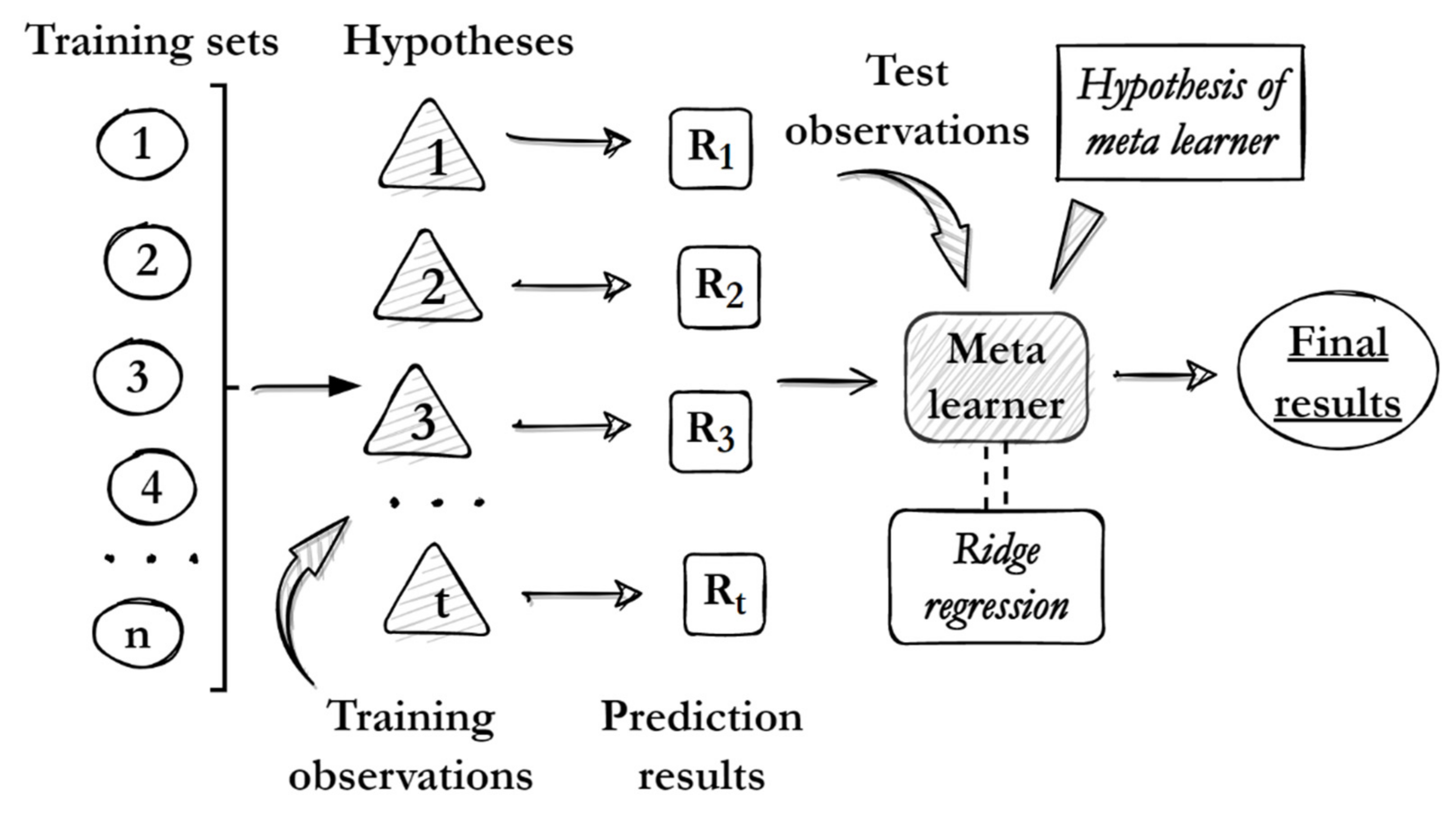
We have compared the prediction performance of various machine learning algorithms, and the results show that ensemble learning is more suitable for predicting the BC emission concentration of diesel engines under steady-state working conditions [36]. However, in this study, we took the performance parameters of the diesel engine as the features of the models. These parameters can describe the performance of diesel engines from a macro perspective, but the correlation between them and BC is weak, and it seems that it is not enough to characterize the BC emission level under the condition of limited training samples. In addition, because there are many kinds of ensemble learning algorithms, choosing the best ensemble algorithm or integrating these algorithms has become a very challenging task. Therefore, in this paper, we propose a new BC emission prediction model for diesel engines, based on a stacked generalization, for the first time, which integrates XGB, LGB, RF, SVR and RR. Stacked generalization is a method to minimize the generalization error of multiple estimators, which can integrate different types of estimators in order to eliminate the bias and non-uniformity of the different algorithms [37,38]. At present, many studies have shown that the model after fusion using stacked generalization has stronger prediction ability than a single model [39,40]. Wu et al. believe that the generation of BC is related to the combustion process, and BC emissions can be reduced by improving the combustion process in the cylinders [41], while the combustion process can usually be described and controlled by combustion characteristic parameters (CCPs) [42,43]. Therefore, in this paper, we have carried out a detailed analysis of the correlation between CCPs and BC emissions, and select them as the features of the prediction models.

The contributions of this paper can be summarized as follows:

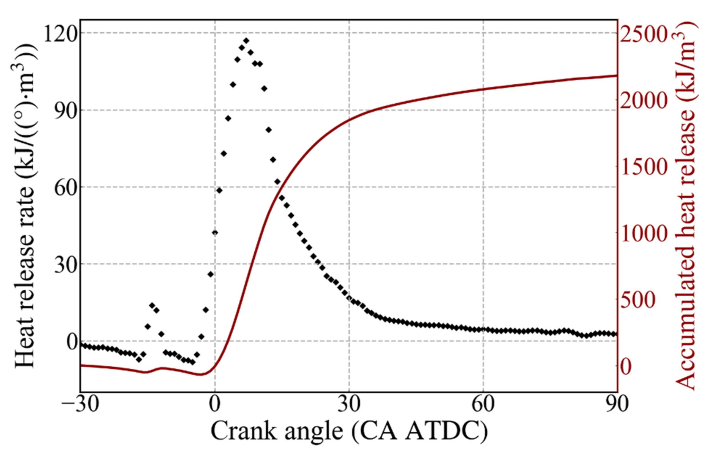
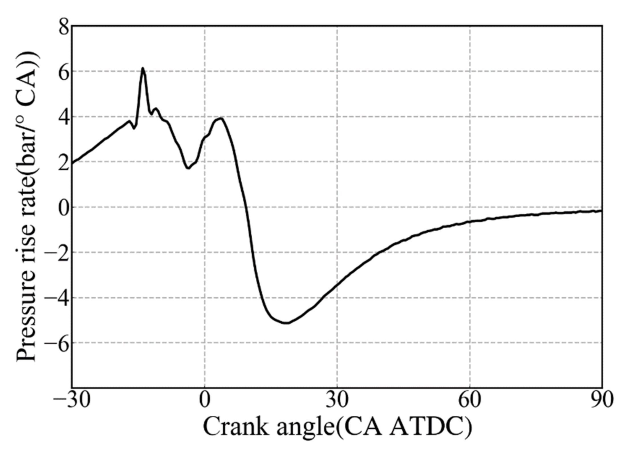
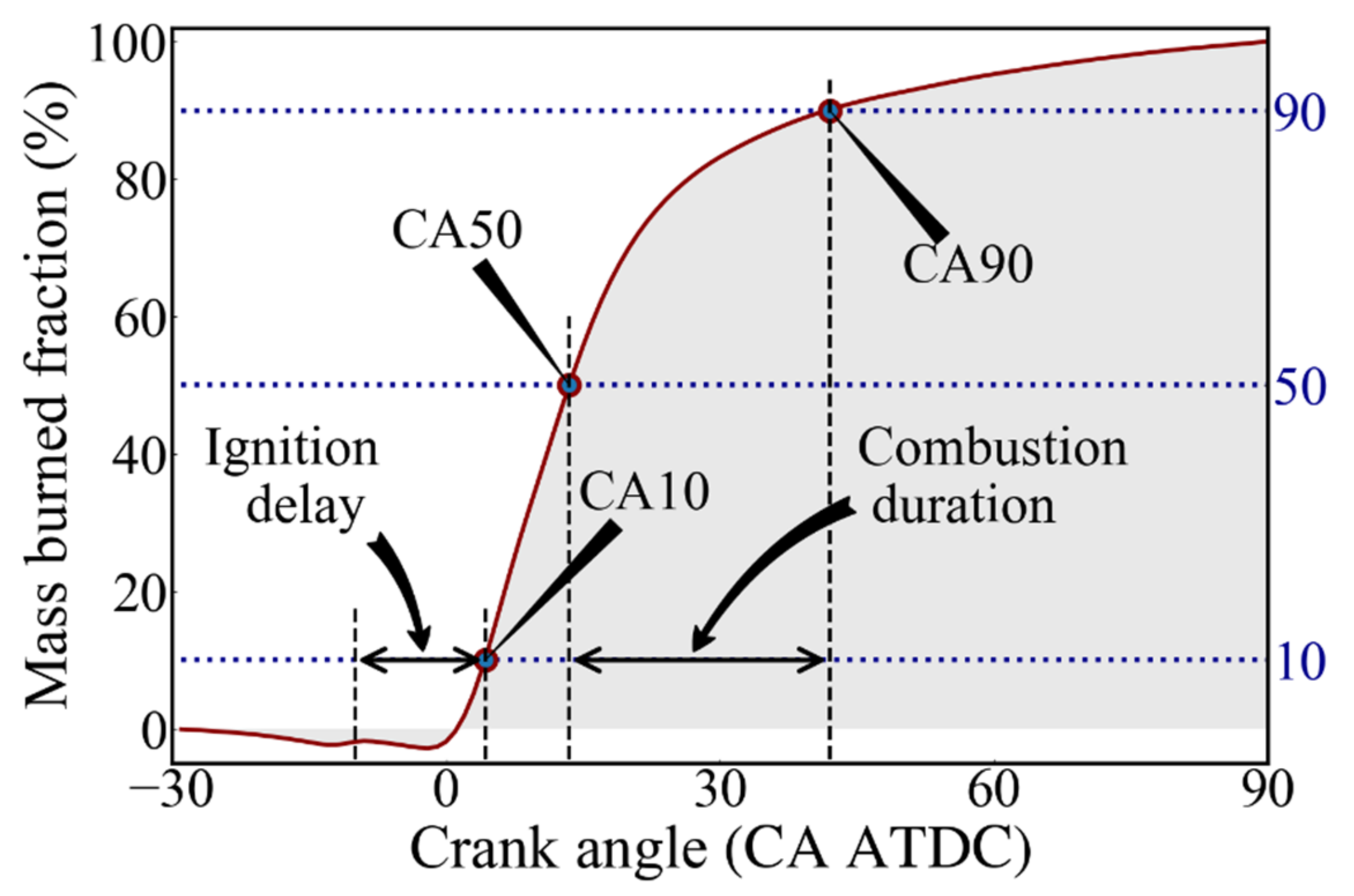
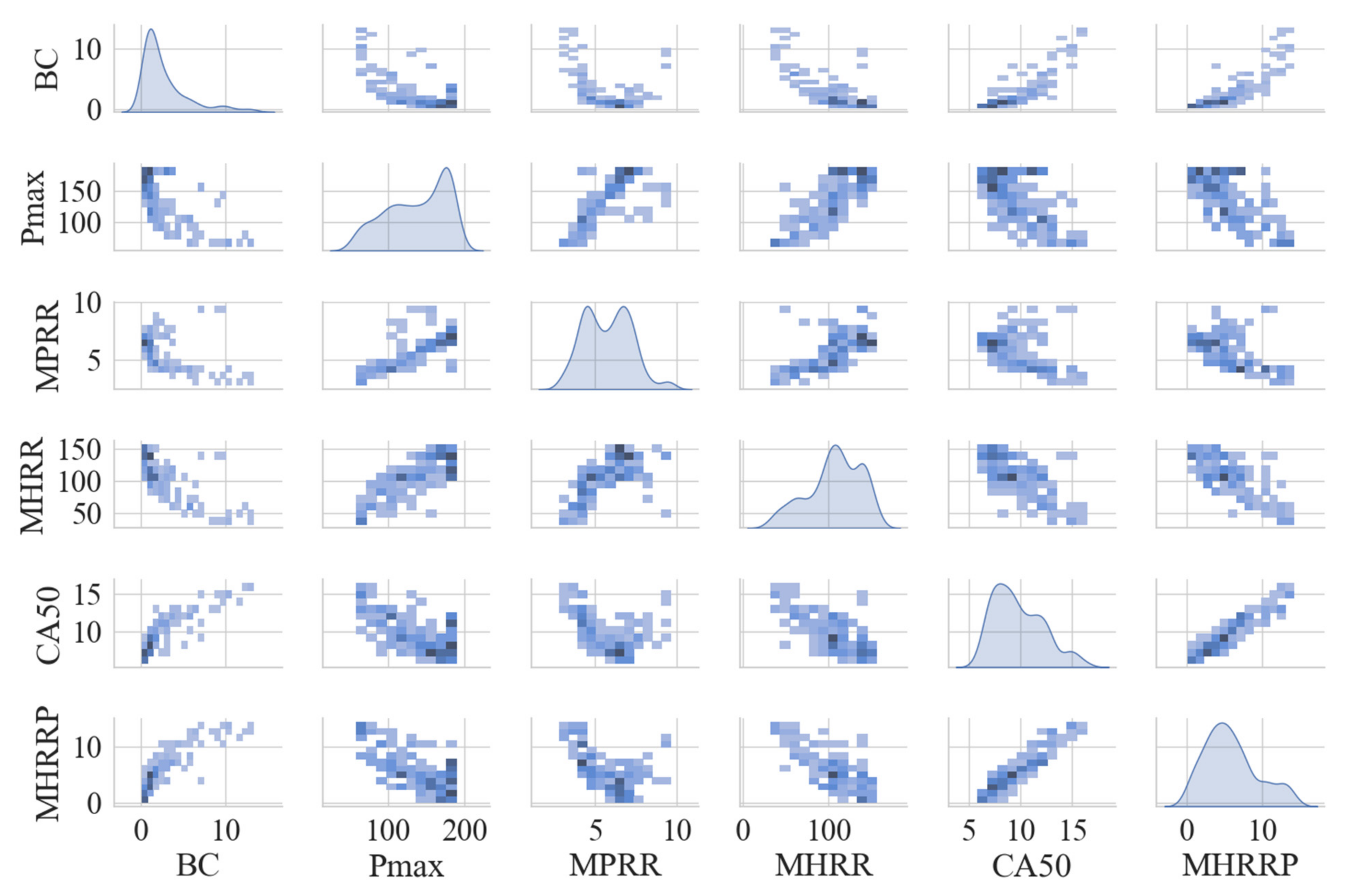
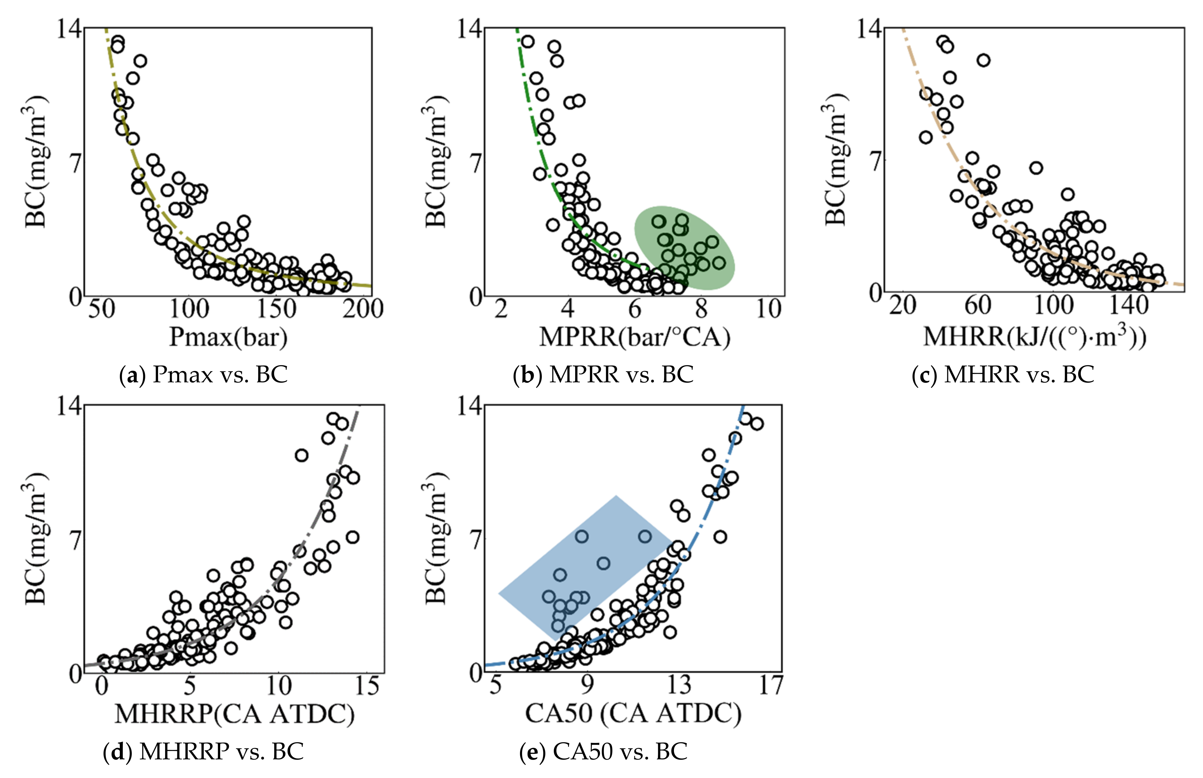
• Pmax (Maximum Cylinder Pressure), MPRR (Maximum Pressure Rise Rate), MHRRP (Maximum Heat Release Rate Phase), MHRR (Maximum Heat Release Rate) and CA50 (Exothermic Center Phase) are extracted from the cylinder pressure data which acquired under different steady-state working conditions of the diesel engine, and then the influences of the changes of these CCPs on the BC emission concentration are theoretically analyzed and explained;
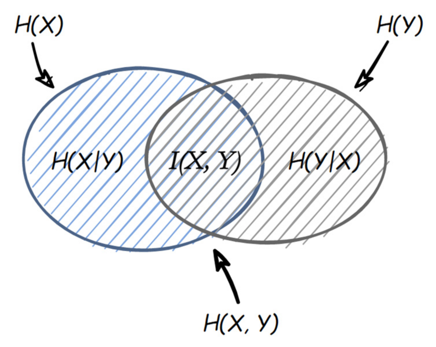
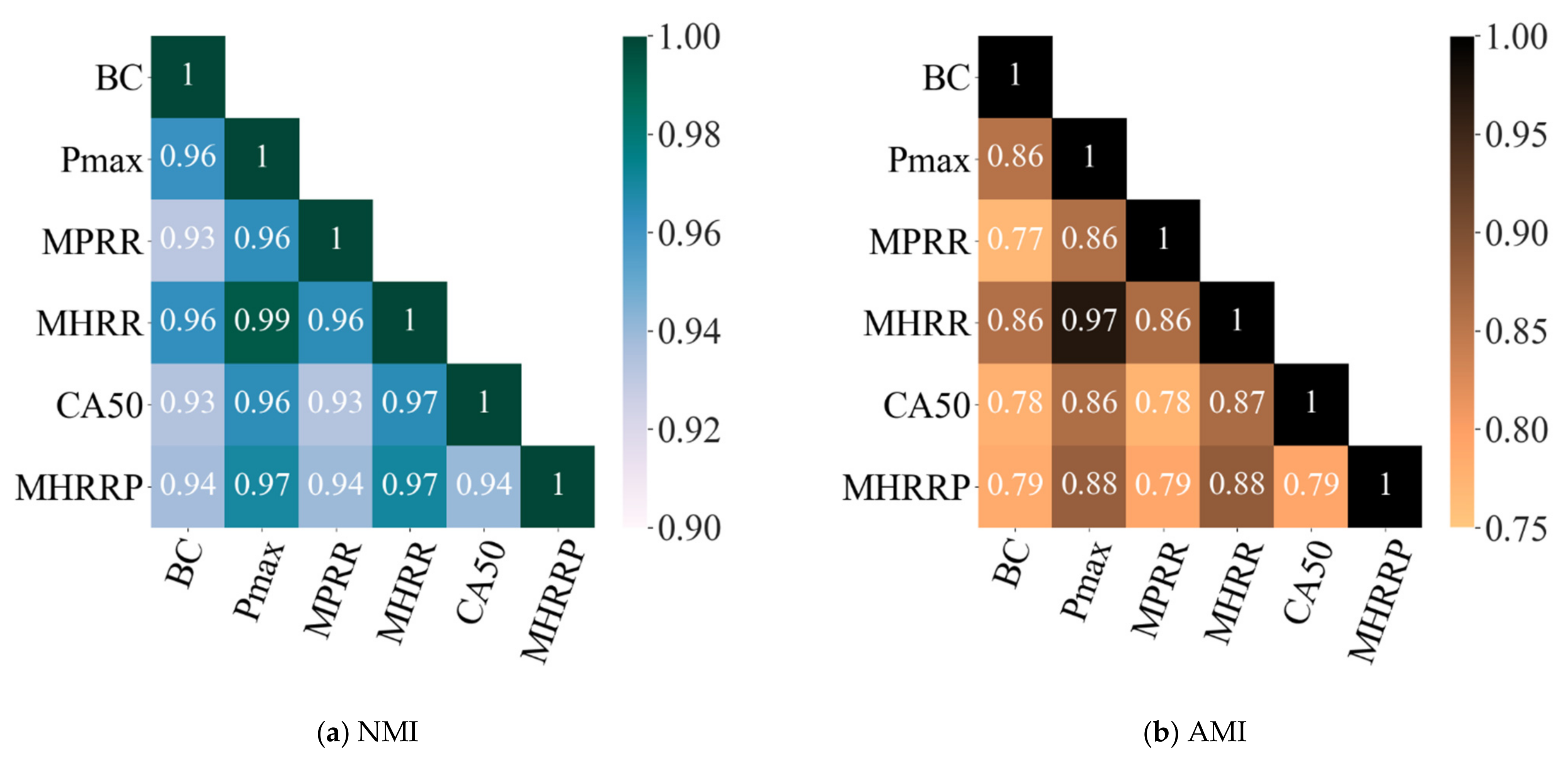
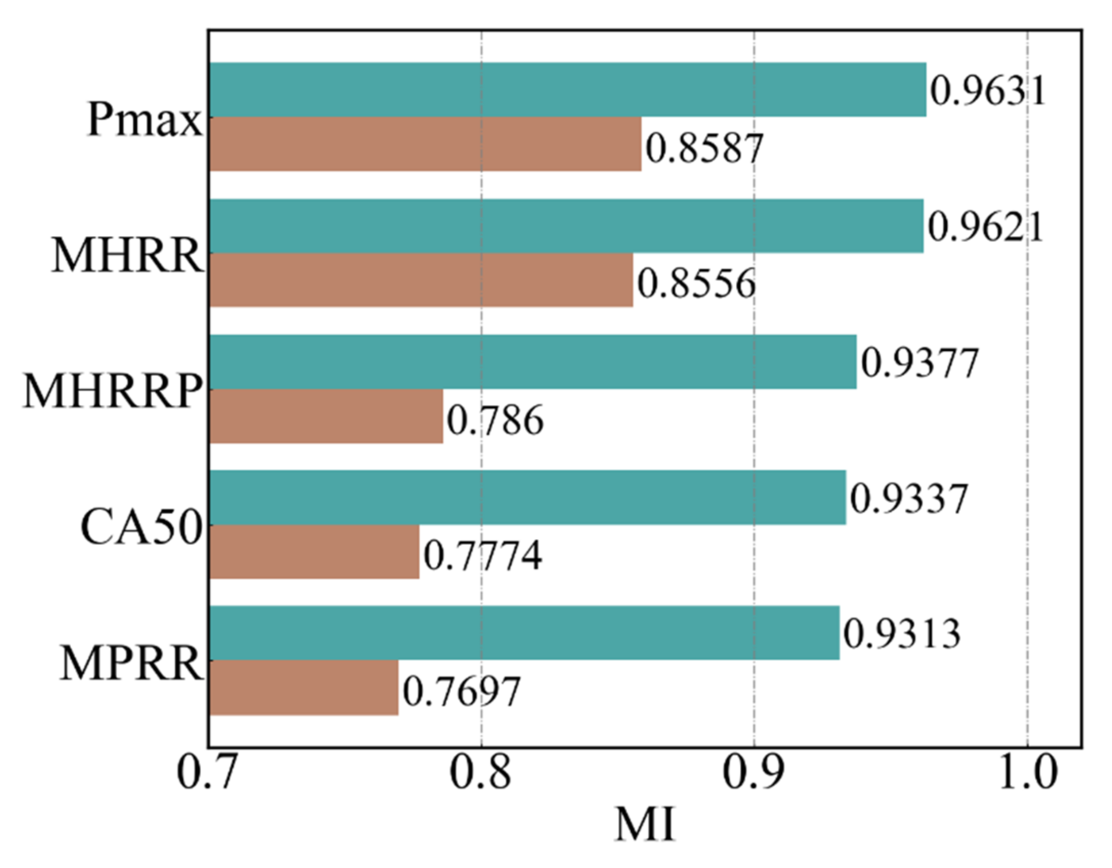
• Mutual information is used to measure the correlation between the CCPs and BC emission concentration. It is found that there is a strong correlation between the CCPs and BC emission concentration. This result fully proves that suitable CCPs can be used as the features of BC emission prediction model;
• A new prediction model of diesel engine BC emissions based on SG is proposed. The stability and prediction accuracy of the SG model are higher than those of its sub models, and it can achieve higher prediction performance when the number of training samples of the model is very limited.

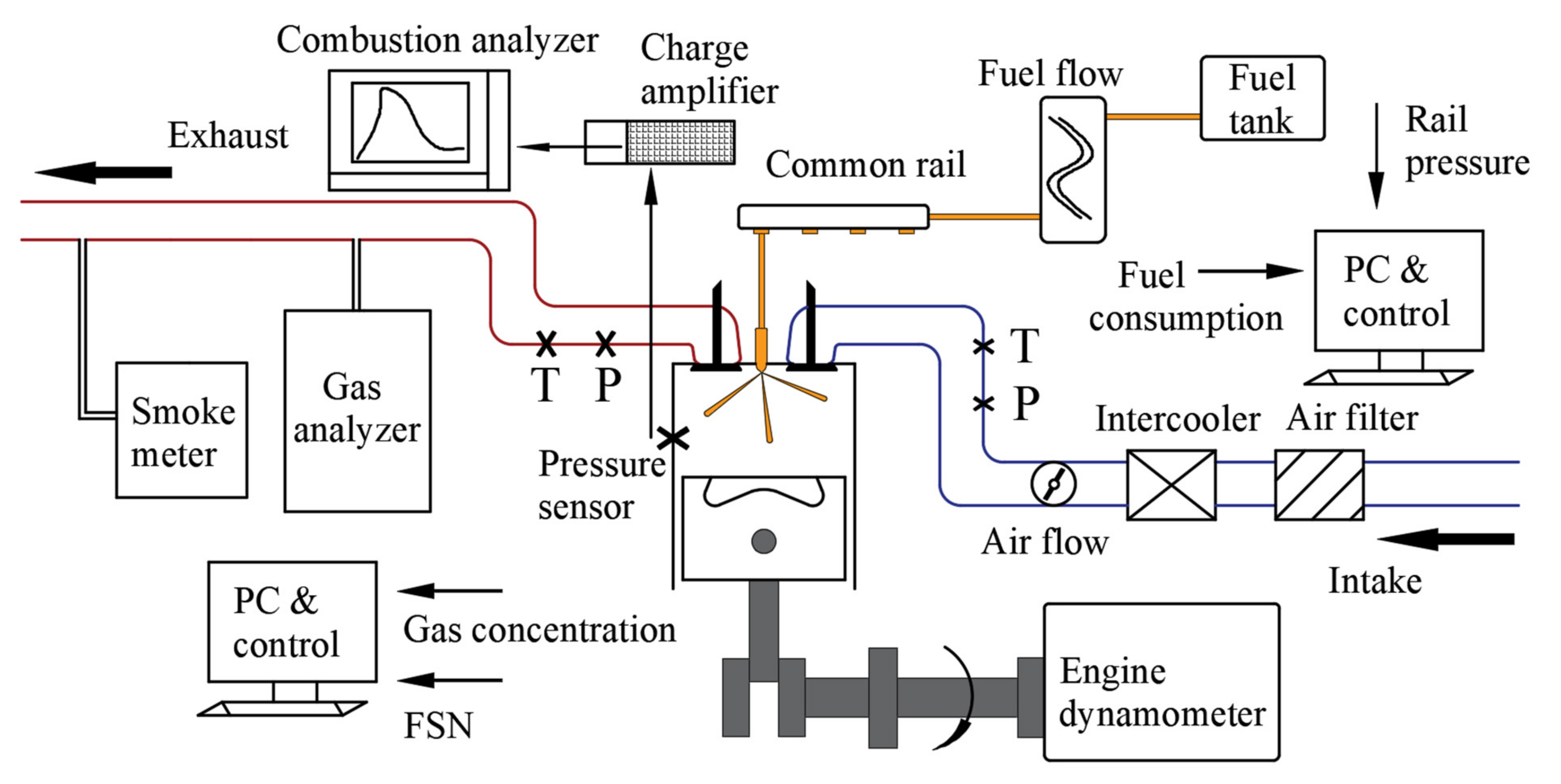
The remainder of the paper is organized as follows: In Section 2, we first describe the test instruments and test methods, then briefly introduce the definition of CCPs and the theory of the machine learning algorithms; Section 3 analyzes the influences of the changes in CCPs on BC concentration, and calculates the correlation between them using mutual information, and then compares and evaluates the prediction performance of each sub model and SG model; In Section 4, we draw conclusions of this paper and some follow-up research plans.

2. Materials and Methods

2.1. Test and Data Acquisition

The test object of this study is a marine high-speed diesel engine. The engine specifications are summarized in

Table 1. Specifications of the test engine.

Description	Specification
Rated power	142 kW
Rated speed	2200 rpm
NO. Cylinder	4
NO. Stroke	4
Displacement	5.1 L
Bore	110 mm
Stroke	135 mm
Compression ratio	19.05
Cylinder arrangement	In-line

.

The schematic diagram of the engine test bench is presented in Figure 1.

In the steady-state tests of the diesel engine, it is necessary to control the environmental variables. The intake air temperature was maintained at ~(25 ± 2) °C by the air conditioner, the air humidity was maintained at about 50%, and the air intake pressure was ~(101 ± 1) kPa. The exhaust pressure of the engine was maintained at ~(10 ± 0.5) kPa. The cooling mode of the engine was water cooling, and the cooling water temperature was maintained at ~(85 ± 5) °C. The fuel used in the tested engine was China VI 0# diesel.

Kistler 6125c cylinder pressure sensor was used for cylinder pressure measurement. The measuring range of Kistler 6125c is 0~300 bar and the deviation is ±1%.

The installation position of the cylinder pressure sensor was located in the cylinder head of the first cylinder and connected with the charge amplifier. The pressure signal was amplified by the charge amplifier and transmitted to the combustion analyzer. In the test, we collected cylinder pressure data within the whole cycle (−360° CA to 360° CA) in the step of 0.5° CA, so 1441 data samples can be collected in each single cycle.

The Electronic Control Unit (ECU) of the engine is used to independently control the operation parameters of the engine, such as rail pressure, injection timing and number of injections. During the tests, only the rail pressure or the main injection timing shall be adjusted under the same working conditions.

Table 2. Variation range of engine test conditions and operating parameters.

	Working Conditions		Operation Parameters
	Speed	Load	Rail Pressure	Injection Timing
Unit	rpm	%	MPa	CA ATDC
Variation range	[700, 2200]	[10, 100]	[40, 160]	[−12, 4]
Interval	100	10	20	2

lists the variation range of engine test conditions and operating parameters.

We use the filter-type smoke meter (AVL 415S) to measure the BC concentration of the engine. According to the international standard ISO 8178-3 [44], the mass concentration of BC is converted by Equation (1):

$$eBC=\frac{1}{0.405}\times FSN\times 5.32\times e^{0.3062\times FSN}$$

(1)

where $eBC$ is the mass concentration of BC, in mg/m³, and FSN is the smoke value measured by AVL 415S.

The specifications of the instruments used on the test bench are summarized in

Table 3. Instruments on the test bench.

Instruments	Type	Deviation
Dynamometer	AVL INDY S22-4	±0.3%
Air flowmeter	ABB-0(40) …1200 kg	±0.1%
Cylinder pressure sensor	Kistler 6125C	±1%
Combustion analyzer	Kistler Kibox	-
Fuel consumption meter	AVL 735S	±0.5%
Smoke meter	AVL 415S	0.1% FSN
Gas analyzer	AMA 4000	±0.5%

.

2.2. Definition and Calculation Method of CCPs

The cylinder pressure contains rich combustion information. Through the test, we collected 161 groups of effective cylinder pressure data and BC emission concentration under corresponding working conditions; Figure 2 shows a group of in-cylinder pressure data measured when the engine speed is 1600 rpm.

In order to obtain the CCPs, it is necessary to calculate the instantaneous heat release rate according to the cylinder pressure. The heat release rate is calculated according to Equation (2):

$$ROHR=\frac{\gamma }{\gamma -1}P\frac{dV}{d\phi }+\frac{1}{\gamma -1}V\frac{dP}{d\phi }-Q_w$$

(2)

where $\gamma$ is the adiabatic index of the mixture in the cylinder, $P$ represents the cylinder pressure, φ is the crank angle. $V$ is the working volume of the cylinder which calculated according to the structural parameters of the engine (bore D, stroke S, connecting rod length L and compression ratio ε). $Q_w$ represents the heat transfer loss of the cylinder, which can be ignored in order to simplify the analysis process.

Then the simplified Equation (2) is discretized. The calculation method of the heat release rate after discretization is shown in Equation (3):

$$ROH{R}_i=[\frac{\gamma }{\gamma -1}{P}_i(V_i-V_{i-1}+\frac{1}{\gamma -1}{V}_i(P_i-P_{i-1}))]/\left({\phi }_i-{\phi }_{i-1}\right)$$

(3)

Accumulated heat release refers to the total heat released at a certain time during the combustion process, which is derived from the accumulation of heat release rate. The calculation method is shown in Equation (4):

$$AH{R}_i=AH{R}_{i-1}+ROH{R}_{i-1}\left({\phi }_i-{\phi }_{i-1}\right)$$

(4)

Figure 3 shows the calculated heat release rate and cumulative heat release.

The Maximum Pressure Rise Rate (MPRR) reflects the change rate of pressure in the cylinder, which has an important impact on the fuel economy, power, vibration and noise of the engine. MPRR is one of the most important CCPs, the calculation method of pressure rise rate is shown in Equation (5):

$${(\frac{dp}{d\phi })}_k=\frac{p_{k+1}-p_{k-1}}{{\phi }_{k+1}-{\phi }_{k-1}}, k=1, 2, 3\dots K$$

(5)

where $p$ is the cylinder pressure, $\phi$ is the crankshaft angle, and $K$ is the serial number of the collected in-cylinder pressure. The MPRR is the maximum value in the rate of change.

As shown in Figure 4, the Pressure Rise Rate changes with the crank angle.

CA50 is also one of the CCPs commonly used to control the combustion process of the engine. It represents the crank angle phase when the heat release in a single working cycle of the diesel engine reaches 50% of the total heat release, and is therefore also called the heat release center phase. The definition of CA50 is shown in Figure 5. CA10, CA50 and CA90 are the corresponding crankshaft angles when the combustion mass fraction reaches 10%, 50% and 90%, respectively. The combustion mass fraction is the proportion of the current accumulated heat release to the total heat release. CA10 and CA90 are, respectively, defined as the starting point and end point of combustion.

2.3. Theory of Algorithms

2.3.1. Extreme Gradient Boosting (XGB)

Boosting aims to promote weak learners to strong learners. The algorithm trains a base learner from the initial training set, and then adjusts the distribution of training samples according to the performance of the base learner. Consequently, samples that were wrongly judged before will receive more attention in the subsequent training, and then uses the adjusted sample distribution to train the next base learner until the number of base learners reaches the set value T, and finally all the base learners are combined by weighting. XGB expands the loss function by second-order Taylor series and introduces the regular term to the loss function to control the complexity of the model [45].

2.3.2. Light Gradient Boosting Machine (LGB)

Similar to XGB, LGB essentially belongs to the boosting algorithm, which can effectively reduce computing costs and improve scalability when solving problems with high feature dimensions and large data size [46]. For each feature, the Gradient Boosted Decision Tree (GBDT) needs to scan all of the training samples in order to estimate the information gain of all possible segmentation points. To solve this problem, LGB introduces two new technologies: GOSS (Gradient based One Side Sampling) and EFB (Exclusive Feature Binding). The advantages of LGB are as follows: 1. It reduces the use of memory by data and ensures that a single machine can use as much data as possible without sacrificing computing speed; 2. It reduces the cost of communication, improves the efficiency when multiple computers are parallel, and achieves linear acceleration in computing.

2.3.3. Random Forest (RF)

RF has the advantages of simplicity, easy implementation, low computational overhead, etc. It is a variant of the parallel ensemble learning method bagging, which is based on bootstrap sampling [47]. That is, given a data set containing m samples, the samples are randomly extracted and put back into the initial data set. After m times of random sampling, the sampling set containing m samples can be obtained. Some samples in the initial data set are sampled multiple times, while others never appear. According to such rules, we can obtain T sampling sets containing m training samples, train a base learner based on each sampling set, and then combine the base learners. The weak learner of RF is CART (Classification and Regression Trees). Based on bagging, it further introduces random attribute selection in the training process of decision tree. Figure 6 is the schematic diagram of boosting and bagging.

2.3.4. Support Vector Regression (SVR)

SVR is one of the most important algorithms in machine learning, and has been widely used because of its high flexibility and generalization ability. The traditional regression algorithm usually calculates the loss directly based on the difference between the output $f\left(x\right)$ of the model and the real value. In contrast, the key of SVR is to build the interval. Only when the absolute value of the difference between the estimated value and the expected value is greater than the tolerance deviation, the loss is calculated. When the sample falls into the interval band of twice the deviation range, the prediction is judged to be correct [48].

The basic type of SVR is:

$$\left\{\begin{array}{c}mi{n}_{w,b}\frac{1}{2}{\Vert w\Vert }^2\\ s.t. y_i\left(w^T+b\right)\ge 1,i=1,2,\dots ,m.\end{array}\right.$$

(6)

The linear regression function of training samples is:

$$L\left(f\left(x\right),y,ϵ\right)=\left\{\begin{array}{c} 0, if \left|y-f\left(x\right)\right|\le ϵ\\ \left|y-f\left(x\right)-ϵ\right|, othrtwise\end{array}\right.$$

(7)

By introducing relaxation variables ${\xi }_i$ and ${\widehat{\xi }}_i$, the problem of finding hyperplane can be expressed as:

$$\left\{\begin{array}{c}mi{n}_{w,b,{\xi }_i,{\widehat{\xi }}_i}\frac{{\Vert w\Vert }^2}{2}+C{\displaystyle \sum _{i=1}^m}({\xi }_i+{\widehat{\xi }}_i)\\ s.t. \left\{\begin{array}{c}f\left(x_i\right)-y_i\le ϵ+{\xi }_i\\ y_i-f\left(x_i\right)\le ϵ+{\widehat{\xi }}_i\\ {\xi }_i\ge 0,{\widehat{\xi }}_i\ge 0,i=1,2,\dots ,m.\end{array}\right.\end{array}\right.$$

(8)

where $w$ is the normal vector of the hyperplane, $b$ defines the distance between the hyperplane and the origin, and $C$ is the penalty factor, $ϵ$ is the error of regression function.

2.3.5. Ridge Regression (RR)

RR is a multiple regression analysis method commonly used in statistics. Compared with the ordinary least squares method, the difference is that the L2 regular term (penalty factor) is introduced into the loss function. In ordinary multiple regression, multiple collinearity problems will occur between features, and the coefficient estimation using the least squares method will be unstable, lacking stability and reliability. The introduction of regular term can effectively alleviate the problem of multiple collinearities, and reduce the complexity of the model to avoid the occurrence of over fitting. The loss function of RR is as Equation (9):

$$L\left(\theta \right)={\displaystyle \sum }_{i=1}^p{\left(y_i-x_i\beta \right)}^2+\lambda {\displaystyle \sum }_{j=0}^n{\beta }_j{}^2$$

(9)

where ${\beta }_p$ represents the coefficient of the $j$-th feature in the total $p$ features. ${\displaystyle \sum }_{j=0}^n{\beta }_j{}^2$ is the penalty term and $\lambda$ is the penalty coefficient, which is used to control the penalty intensity for ${\beta }_j$. The larger the value of $\lambda$ is, the simpler the generated model will be.

2.3.6. Stacked Generalization (SG)

SG is an efficient ensemble algorithm, and was first proposed by Wolpert [49]. The greatest difference between SG and homologous ensemble algorithms, such as bagging or boosting, is that it is composed of heterogeneous estimators. Since each machine learning algorithm uses different methods to represent the knowledge and bias learned from the data, they will explore the hypothesis space from different perspectives to determine the optimal model. In order to combine the prediction results of various algorithms and eliminate the inherent bias of the algorithm, SG adopts a stacking strategy. As shown in Figure 7, the basic learners of SG model in this paper are LGB, RF, XGB and SVR. In order to avoid serious over fitting, the simpler linear regression model RR is used as the meta learner, and the stacked model is ensembled by taking the output of the basic learner as the input of the meta learner.

The following Algorithm 1 is the flow of SG algorithm:

Algorithm 1: Stacked Generalization [49]

Input: Training data $\mathcal{D}={\left\{x_i,y_i\right\}}_{i=1}^m\left(x_iϵ{ℝ}^n,y_iϵ\mathcal{Y}\right)$

Output: An ensemble regressor H

Step1: Learn base regressors

1: $for t=1,2,\dots ,T do$

2:     Learn a base regressor $h_t$ based on $\mathcal{D}$

3: $end for$

Step 2: Construct new datasets from $\mathcal{D}$

4: $for i=1,2,\dots ,m do$

5:     Construct a new dataset that contains $\left\{x_i^{\prime },y_i\right\}$, where $x_i^{\prime }=\left\{h_1\left(x_i\right),h_2\left(x_i\right),\dots ,h_T\left(x_i\right)\right\}$

6: $end for$

Step 3: Learn meta regressor

7: Learn a new regressor $h^{\prime }$ based on the newly constructed dataset

8: $return H\left(x\right)=h^{\prime }\left(h_1\left(x\right),h_2\left(x\right),\dots ,h_T\left(x\right)\right)$

2.3.7. Mutual Information (MI)

MI, derived from information theory, is an effective information measurement method, which can be used to measure the correlation between nonlinear parameters to achieve the effect of feature recognition or clustering. This method is widely used in the field of data science [50]. Figure 8 is a schematic diagram of MI.

Suppose that there are sets $X=\left\{x_1,x_2,\dots , x_R\right\}$, $Y=\left\{y_1,y_2,\dots , y_C\right\}$, and the proportion of class $k$ samples in $X$ is $p_k\left(k=1,2,\dots ,R\right)$, then the information entropy of $X$ is:

$$Ent\left(X\right)=-{\displaystyle \sum }_{k=1}^R{p}_{k}lo{g}_2{p}_k$$

(10)

Let the joint distribution of discrete random variables $X$ and $Y$ be $p\left(x,y\right)$, then the marginal distributions of $X$ and $Y$ are $p\left(x\right)$ and $p\left(y\right)$, and the mutual information is the relative entropy of the joint distribution $p\left(x,y\right)$ and the marginal distributions $p\left(x\right)$ and $p\left(y\right)$:

$$MI\left(X,Y\right)={\displaystyle \sum }_{x,y}p\left(x,y\right)log\frac{P\left(x,y\right)}{p\left(x\right)p\left(y\right)}$$

(11)

In order to scale the mutual information between [0, 1], it is necessary to normalize the mutual information according to Equation (12):

$$NMI\left(X,Y\right)=\frac{MI\left(X,Y\right)}{F\left(H\left(X\right),H\left(Y\right)\right)}$$

(12)

However, for discrete variables, if the values of $X$ and $Y$ are more, the mutual information $NMI\left(X,Y\right)$ tends to become grater, but this is not caused by the strong correlation between $X$ and $Y$. Adjusted Mutual Information (AMI) eliminates the above effects. The calculation of AMI is as Equation (13):

$$AMI\left(X,Y\right)=\frac{MI\left(X,Y\right)-E\left\{MI\left(X,Y\right)\right\}}{F\left(H\left(X\right),H\left(Y\right)\right)-E\left\{MI\left(X,Y\right)\right\}}$$

(13)

where $E\left\{MI\left(X,Y\right)\right\}$ is the expectation of MI of variables $X$, $Y$.

$$\begin{gathered} E\left\{MI\left(X,Y\right)\right\}= \\ {\displaystyle \sum }_{i=1}^x{\displaystyle \sum }_{j=1}^y{\displaystyle \sum }_{k={\left(a_i+b_j-N\right)}^{+}}^{\min \left(a_i,b_j\right)}\frac{k}{N}\log \left(\frac{N\times k}{a_i\times b_j}\right)\frac{a_i!b_j!\left(N-a_i\right)!\left(N-b_j\right)!}{N!k!\left(a_i-k\right)!\left(b_j-k\right)!\left(N-a_i-b_j+k\right)!} \end{gathered}$$

(14)

where $N$ is the number of all variables in set $X$ and set $Y$. ${\left(a_i+b_j-N\right)}^{+}$ denotes $max{\left(a_i+b_j-N\right)}^{+}$.The variables $a_i$ and $b_j$ are partial sums of the contingency table.

In this paper, $F\left(H\left(X\right),H\left(Y\right)\right)$ is selected as the arithmetic average, so $NMI$ and $AMI$ are shown in Equations (15) and (16):

$$NMI\left(X,Y\right)=\frac{MI\left(X,Y\right)}{\frac{1}{2}\left(H\left(X\right)+H\left(Y\right)\right)}$$

(15)

$$AMI\left(X,Y\right)=\frac{MI\left(X,Y\right)-E\left\{MI\left(X,Y\right)\right\}}{\frac{1}{2}\left(H\left(X\right)+H\left(Y\right)\right)-E\left\{MI\left(X,Y\right)\right\}}$$

(16)

3. Results and Discussion

3.1. Influence of Combustion Process Change on BC Emission Concentration

The key to improving the power and emissions performance of diesel engines is to optimize and control the combustion process in the cylinder. Therefore, the research on the new combustion modes of diesel engines and combustion systems of new clean fuel has received extensive attention [51,52,53]. If the combustion path of the diesel engine can be effectively controlled, so that the working medium can burn efficiently in the cylinder, then the pollutant emission concentration will be significantly reduced [54]. We believe that the change in the combustion process has an important influence on the generation and emission of BC, and selecting CCPs that can describe the combustion process as the features of BC emission prediction model can not only improve the prediction performance of the model, but also provide a meaningful reference for the application of combustion control technology. In this paper, five commonly used CCPs are selected as research objects: Maximum Cylinder Pressure (Pmax), Maximum Pressure Rise Rate (MPRR), Maximum Heat Release Rate (MHRR), Maximum Heat Release Rate Phase (MHRRP) and Heat Release Center Phase (CA50).

Figure 9 shows the relationship between CCPs and BC concentrations in pairs, and the graph on the diagonal represents the distribution of each parameter. Figure 9 shows that there are obvious correlation trends between the parameters. For example, it can be seen that CA50 and MHRRP have a highly linear positive correlation, because both are directly affected by the fuel injection time and injection pressure. This result also confirms the accuracy of our parameter calculation results. However, the relationship between most parameters is not a simple linear correlation, and as there are 161 groups of valid data, the pixel-based distribution map cannot accurately depict the local details in the figure, so we will use the scatter map for further discussion.

Figure 10 shows the scatter plot of CCPs and BC concentrations under different working conditions. It can be seen from Figure 10a–c that with the increase of Pmax, MPRR and MHRR, the BC concentration shows a significant downward trend.

Pmax is primarily related to the total amount of premixed working medium formed during the ignition delay period, and the total amount of premixed working medium will be affected by factors such as the fuel injection amount, fuel properties, and cylinder air flow strength [55]. The increase in Pmax means that the proportion of fully oxidized fuel increases, thus reducing the BC concentration. Similar to Pmax, MHRR is related to the cylinder pressure and combustion chamber volume [56]. The larger the MHRR, the greater the proportion of the ignition delay period in the combustion duration will be, this, in turn, speeds up the conversion rate from fuel to energy, and renders the maximum drop rate of BC at more than 90%.

It can be seen from the green oval area in Figure 10b that with the increase in MPRR, the BC concentration rises, slightly, from the lowest point. The increase in MPRR indicates that the turbulence of the working medium is more intense, the flame propagation speed is increased [57,58], and this inhibits the generation process of black BC caused by local hypoxia, thus greatly reducing the BC concentration. However, with the continuous increase in MPRR, there is a pressure difference in the combustion chamber at the same time, resulting in pressure oscillations, which aggravates the combustion process in the cylinder, and the diesel engine cannot run smoothly [59]. The obvious inflection point occurs when MPRR is 6 bar/° CA. After the inflection point, the BC concentration increased significantly, from 1.4 mg/m³ to 6.2 mg/m³.

The MHRRP is affected by the injection timing and the starting point of combustion, and also has a clear positive correlation with CA50. It can be seen from Figure 10d that the earlier MHRRP occurs, the more forward the starting point of combustion is, the more combustible mixture is formed during the ignition delay period, and the lower the BC concentration is.

CA50 is primarily affected by the injection timing and injection pressure [54,60,61,62]. Figure 10e shows that when CA50 is forward, the diffusion combustion duration is relatively short, and the BC concentration is relatively small. It is worth noting that, as shown in the data of the blue rectangular area in the figure, under some working conditions, the delay of injection timing (delay of CA50) shortens the mixing time of oil and gas, and more fuel forms BC through incomplete combustion, so the BC concentration will increase.

3.2. Correlation Analysis between CCPs and BC

Correlation analysis is an important prerequisite for establishing efficient prediction models. Scientists usually use correlation coefficients to perform correlation analysis on different parameters [53,63]. However, correlation coefficients cannot measure complex nonlinear relationships. In addition, MI has been proven to be a better and more accurate measurement method. Therefore, this paper uses MI theory for correlation analysis. Figure 11a,b shows the NMI and AMI between the parameters, respectively. The color blocks in the figure represent the MI between different parameters. The darker the color of the color blocks, the stronger the correlation between the parameters. It can be seen from Figure 11 that Pmax and MHRR have the strongest correlation, with NMI and AMI reaching 0.99 and 0.97, respectively. Moreover, BC has a high correlation with various CCPs, which is shown in Figure 12.

Figure 12 shows the MI values between CCPs and BC concentrations. The green columns in the figure represent the NMI value, while the brown columns represent the AMI value. It can be seen from the figure that the NMI between the CCPs and BC concentrations are greater than 0.9, while the AMI are greater than 0.75. The AMI are smaller than the NMI, indicating that the AMI reduces the measurement deviation of NMI due to multiple variable values [64,65]. The correlations between CCPs and BC concentrations are strong, and the AMI between Pmax and MHRR and BC concentrations are significantly higher than the other three parameters (0.8587 and 0.8556). Therefore, the selected CCPs can all be used as the feature of BC prediction model.

In addition, because BC concentration is measured under different steady state working conditions of the diesel engine, in order to accurately predict BC concentration, it is necessary to add speed, torque, power and fuel consumption, which can describe the working conditions as the feature of the prediction model.

3.3. Prediction of BC Concentration

Generally speaking, using machine learning to solve regression problems includes four steps: data cleansing, split of dataset, adjustment of hyper parameters, and model performance evaluation. Figure 13 is the flow diagram of establishing the prediction model. We use Python to complete the establishment of BC emission prediction model, and the compilation environment is Pycharm. Python libraries used in modeling include scikit-learn, pandas, numpy and matplotlib.

3.3.1. Split and Preprocessing of Dataset

According to the diesel engine steady state condition test described above, 161 groups of raw data that can be used to train and test the prediction model are finally collected after removing missing and invalid data. Divide the training set and the test set according to the proportion of 8:2, set 121 samples for the training set and 30 samples for the test set. Then, set the remaining 10 groups of samples as the validation set; the samples of the validation set are randomly selected from the original data, and the samples are evenly distributed according to the numerical value.

The algorithm using gradient descent requires feature scaling. The reason for this is that when the data dimensions are inconsistent, the contour of the loss function is an ellipse with a very high eccentricity, which will lead to very complex calculations and will not achieve convergence. After feature scaling, the contour of the loss function tends to be circular, prompting the algorithm to iterate toward the origin, thus effectively reducing the number of iterations. The use of SVR and RR requires feature scaling, while XGB, LGB and RF composed of tree structures do not require feature scaling. The tree model is formed by finding the optimal split point. The numerical scaling of samples does not affect the location of the split point, so it does not affect the structure of the tree model.

The common feature scaling method is normalization, which makes features dimensionless and scales their values to [0, 1]:

$$\widehat{x}=\frac{x-x_{min}}{x_{max}-x_{min}}$$

(17)

where $x$ is the raw data and $x_{min}$ is the minimum value of the feature; $x_{max}$ is the maximum value of the feature; $\widehat{x}$ is the data after normalization.

Table 4. Data information after normalization.

Items	Features
	Pmax	MPRR	MHRR	CA50	MHRRP	Speed	Torque	Power	FC
max	1	1	1	1	1	1	1	1	1
mean	0.598	0.430	0.597	0.370	0.404	0.575	0.524	0.446	0.421
std	0.297	0.212	0.249	0.229	0.249	0.266	0.314	0.283	0.262
min	0	0	0	0	0	0	0	0	0
25%	0.361	0.242	0.451	0.181	0.222	0.333	0.233	0.223	0.214
50%	0.650	0.425	0.629	0.331	0.364	0.600	0.551	0.409	0.371
75%	0.890	0.582	0.824	0.536	0.538	0.800	0.805	0.675	0.598
count	161	161	161	161	161	161	161	161	161

lists the information of the normalized features.

3.3.2. Evaluation Criteria of the Model

In statistics, there are various statistical metrics used to evaluate the prediction performance of the model. This paper used four common metrics. These metrics are Mean Square Error (MSE), Root Mean Squares Error (RMSE), Mean Absolute Error (MAE), and Coefficient of Determination (R²). The equations and performance criteria of these metrics are shown in

Table 5. Evaluation metrics of the model.

Metric	Equation 1	Performance Criteria
MSE	$\frac{1}{n}{\displaystyle \sum _{i=1}^n}{\left({\widehat{y}}_i-y_i\right)}^2$	The smaller the MSE value, the higher the prediction accuracy of the model. The value range of MSE is [0, +∞].
RMSE	$\sqrt[2]{\frac{1}{n}{\displaystyle \sum _{i=1}^n}{\left({\widehat{y}}_i-y_i\right)}^2}$	RMSE is the arithmetic square root of MSE.
MAE	$\frac{1}{n}{\displaystyle \sum _{i=1}^n}\left|{\widehat{y}}_i-y_i\right|$	When the predicted value is completely consistent with the actual value, MAE is equal to 0. The greater the error, the greater the MAE, and the value range of MAE is [0, +∞].
R2	$\frac{{{\displaystyle \sum }}_{i=1}^n{\left({\widehat{y}}_i-\overline{y}\right)}^2}{{{\displaystyle \sum }}_{i=1}^n{\left(y_i-\overline{y}\right)}^2}$	The value range of R2 is [0, 1]. The closer it is to 1, the stronger the model’s ability to explain the predicted object. The closer it is to 0, the worse the fit of the model.

¹  ${\widehat{y}}_i$ is the predicted value, $y_i$ is the true value and $\overline{y}$ is the average of the true values.

.

3.3.3. Analysis of Prediction Results

The quality of the data determines the upper limit of the prediction performance of the models, and the purpose of adjusting the hyper parameters is to ensure the prediction capability of the models approach the upper limit as much as possible. In the process of establishing the model, adjusting the hyper parameters is the most time-consuming step, besides preprocessing. Since there is no reliable theoretical basis for the selection of hyper parameters of the model, most operations can only rely on the intuition and experience of data scientists.

We use grid search to optimize the hyper parameters. Grid search is one of the most basic hyperparameter optimization algorithms. The basic principle is to adjust the parameters sequentially in steps within the specified parameters range, and use the adjusted parameters to train the prediction model until the optimal hyper parameters are found [66,67].

We define the search range of the hyper parameters of different models and take the MSE of the model on the test set as the optimization goal. The hyper parameters of the models, search range and final optimization results are listed in

Table 6. Hyper parameters of the models.

Hyper Parameters	Search Range	Algorithm
		XGB	LGB	RF	SVR	RR
max_depth	[1, 10]	10	7	9	/	/
n_estimators	[10, 1000]	970	1000	980	/	/
eta	[0.01, 0.3]	0.2	/	/	/	/
min_child_weight	[1, 10]	4.3	/	/	/	/
gamma	[0.01, 0.3]	0.001	/	/	0.002	/
num_leaves	[10, 100]	/	21	/	/	/
learning_rate	[0.1, 1]	/	0.7	/	/	/
min_data_in_leaf	[10, 20]	/	17	/	/	/
min_sum_hessian_in_leaf	Default	/	0.001	/	/	/
min_samples_split	Default	/	/	2	/	/
min_samples_leaf	Default	/	/	1	/	/
C	[1, 12]	/	/	/	9	/
epsilon	[0.001, 0.2]	/	/	/	0.01	/
alpha_	[10−7, 102]	/	/	/	/	7.62

.

In order to evaluate the prediction performance of the model, the raw data set is randomly divided into training set and test set, according to the proportion of 8:2; then, each model is trained and tested separately, and the MSE of the model for the test sets is calculated and recorded. We repeated the above steps 299 times, and the final results are shown in Figure 14. It can be seen from the figure that the average MSE of XGB, LGB, SVR, RF and SG are 0.0532, 0.0566, 0.1074, 0.0831 and 0.0485, respectively. The SG model has achieved the best prediction result of all models. When facing different test sets, the prediction results are more stable because of the small variance. In addition, LGB has achieved the lowest variance outside SG, and its prediction performance and stability are better than other algorithms. Many studies have also obtained similar conclusions [68,69,70].

Table 7. Prediction performance evaluation results of each model.

Models	MSE		RMSE		MAE		R2
	Test	Training	Test	Training	Test	Training	Test	Training
XGB	0.0563	0.0033	0.2373	0.0574	0.1630	0.0133	0.9964	0.9996
LGB	0.0537	0.0041	0.2317	0.0640	0.1413	0.0105	0.9941	0.9999
SVR	0.1189	0.0283	0.3448	0.1682	0.1977	0.0875	0.9768	0.9977
RF	0.0822	0.0219	0.2867	0.1480	0.3123	0.1459	0.9779	0.9984
SG	0.0470	0.0016	0.2168	0.0403	0.1175	0.0087	0.9983	0.9999

lists the evaluation results of the prediction performance of each model. The scores of XGB and LGB are relatively close, and their R² for the test set are more than 0.995. The prediction effect of RF and SVR is relatively poor. Their MSE for the training set and test set are relatively larger, and their R² are less than 0.98. SG has the best prediction results among them, with scores higher than the other models. This result proves the effectiveness of the model fusion method, and achieves a high degree of fitting for both test sets and training sets. It is not difficult to see that, compared with our previous research results, this paper uses new features and less training data, but has achieved better prediction results [36].

As the 10 groups of samples in the validation set are independent of the training set and the test set, the prediction of the validation set can more effectively reflect the real prediction ability of the model [71]. The prediction results of each model on the validation set are shown in Figure 15. The average relative error of each model on the validation set is marked in the lower right corner of the figure. From the prediction results of each model on the validation set, it can be seen that the prediction results of SVR are poor, the average relative error exceeds 20%, the prediction results of XGB and LGB are similar, the average relative errors are 14.48% and 13.42%, respectively, while SG has also reached a very high prediction accuracy on the validation set, and the average relative error for each sample is only 10.17%.

Figure 16 shows the relative errors of SG and LGB for each sample in the validation set. It can be seen that the relative errors of SG on the validation set are predominantly less than 15%, while the maximum relative errors of LGB on the validation set samples are more than 30%. The maximum difference between the prediction errors of the two models in all samples is 20.62%. SG can predict samples with smaller values more accurately, which is also SG’s advantage over other models. It can accurately capture the differences between samples and accurately predict smaller values.

4. Conclusions

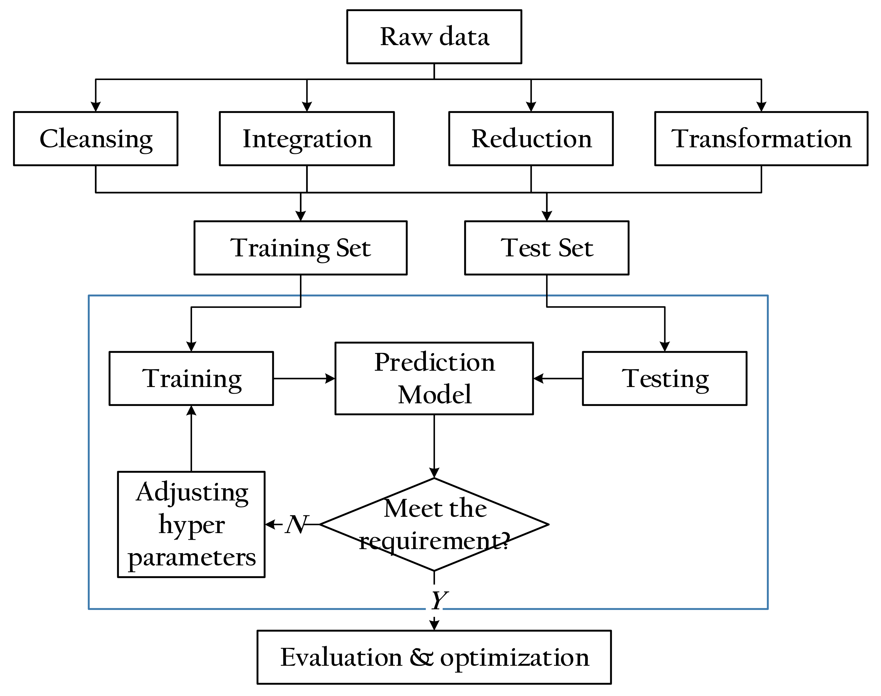
In order to accelerate the research and development process of BC emission control technology for marine diesel engines, this paper proposes an SG-based BC emission prediction model for marine diesel engines, which combines five machine learning models: XGB, LGB, RF, SVR and RR. CCPs with a high correlation with BC emissions are taken as the features of the model. Finally, by comparing the prediction results of the single model and fusion model on the same datasets, the effectiveness of the method is proved. The main research conclusions of this paper are as follows:

• Due to the improvement of fuel utilization efficiency, the increase in Pmax, MPRR and MHRR will reduce the BC concentration; however, with the shortening of the ignition delay period and uneven fuel diffusion, the delay of MHRRP and CA50 led to a significant increase in BC concentration;
• The correlation analysis results show that the NMI between the CCPs and BC concentrations are higher than 0.9, while the AMI are higher than 0.75, which proves that there is a strong correlation between the CCPs and BC concentrations;
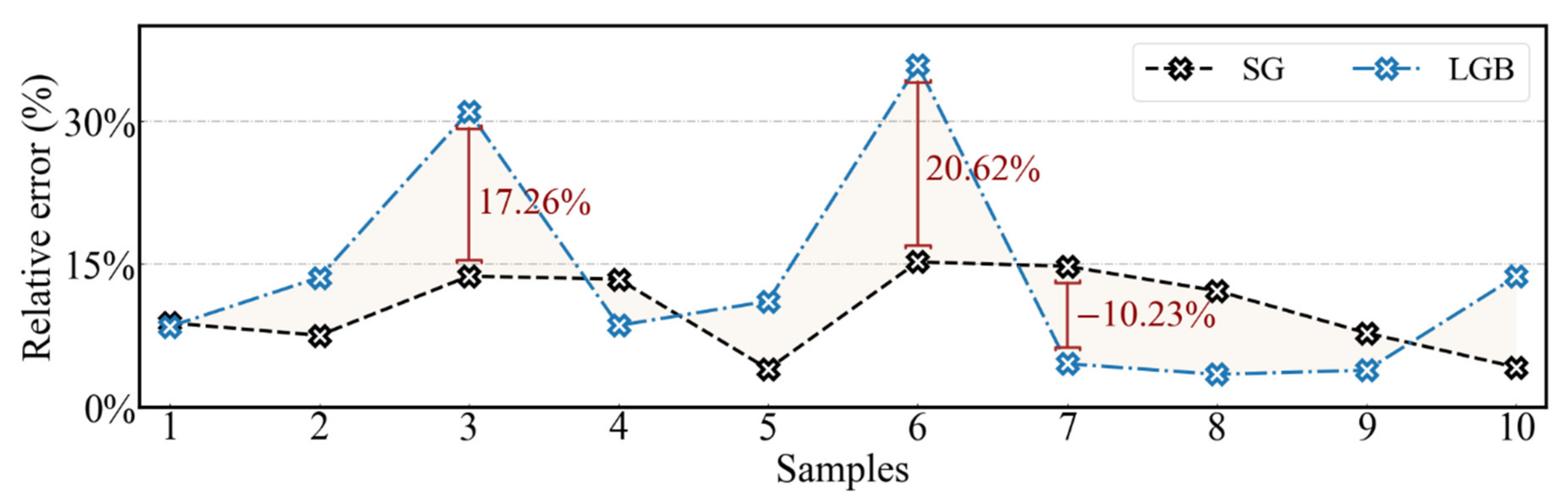
• The fused model reconciles the inherent bias of a single model to data, and achieves the best prediction effect on the different data sets. The MSE and R² of SG model for the test set are 0.0485 and 0.9983, respectively, and its average relative error for validation set is only 10.17%.

As mentioned in the introduction of this paper, machine learning is a cutting-edge data science technology, which can play a very prominent role in engine pollutant prediction. In the future, this technology can also be used to reduce the calculation cost of engine numerical simulation, adaptive control and the construction process of combustion reaction mechanism and other fields.

In addition, the limitations of the method proposed in this paper and the research that can be carried out in the future are: (1) The data used in this paper only comes from one diesel engine, and subsequent tests should be carried out on different types of diesel engines to verify the universality of the conclusions in this paper; (2) The method proposed in this paper can only be used to predict the black carbon emission concentration of engines under steady state conditions (marine engines are more often under steady state conditions), and the prediction of BC emission of diesel engine under transient condition should be discussed in the future; (3) In practical application, the available effective data may be less, so a small sample size BC emission prediction model can be developed to solve the problem.

References

1. Zhu, X.J.; Qian, Y.; Li, X.Q. Research status of black carbon aerosols: Definition and impact on health and climate. Res. Environ. Sci. 2021, 34, 2536–2546. [Google Scholar]
2. Lian, F.; Xing, B. Black carbon (biochar) in water/soil environments: Molecular structure, sorption, stability, and potential risk. Environ. Sci. Technol. 2017, 51, 13517–13532. [Google Scholar] [CrossRef] [PubMed]
3. Klimont, Z.; Kupiainen, K.; Heyes, C. Global anthropogenic emissions of particulate matter including black carbon. Atmos. Chem. Phys. 2017, 17, 8681–8723. [Google Scholar] [CrossRef] [Green Version]
4. Fawole, O.G.; Cai, X.M.; MacKenzie, A.R. Gas flaring and resultant air pollution: A review focusing on black carbon. Environ. Pollut. 2016, 216, 182–197. [Google Scholar] [CrossRef]
5. Gustafsson, Ö.; Ramanathan, V. Convergence on climate warming by black carbon aerosols. Proc. Natl. Acad. Sci. USA 2016, 113, 4243–4245. [Google Scholar] [CrossRef] [Green Version]
6. Bond, T.C.; Doherty, S.J.; Fahey, D.W. Bounding the role of black carbon in the climate system: A scientific assessment. J. Geophys. Res. Atmos. 2013, 118, 5380–5552. [Google Scholar] [CrossRef]
7. Li, C.; Bosch, C.; Kang, S. Sources of black carbon to the Himalayan–Tibetan Plateau glaciers. Nat. Commun. 2016, 7, 12574. [Google Scholar] [CrossRef] [Green Version]
8. Brewer, T.L. Black carbon problems in transportation: Technological solutions and governmental policy solutions. In MIT CEEPR Conference; MIT Center for Energy and Environmental Policy Research: Cambridge, MA, USA, 2017. [Google Scholar]
9. Anenberg, S.C.; Miller, J.; Henze, D.K. The global burden of transportation tailpipe emissions on air pollution-related mortality in 2010 and 2015. Environ. Res. Lett. 2019, 14, 094012. [Google Scholar] [CrossRef]
10. Zhu, Y.; Zhou, W.; Xia, C. Application and Development of Selective Catalytic Reduction Technology for Marine Low-Speed Diesel Engine: Trade-Off among High Sulfur Fuel, High Thermal Efficiency, and Low Pollution Emission. Atmosphere 2022, 13, 731. [Google Scholar] [CrossRef]
11. Comer, B.; Olmer, N.; Mao, X. Black Carbon Emissions and Fuel Use in Global Shipping 2015; International Council on Clean Transportation: Washington, DC, USA, 2017. [Google Scholar]
12. Sand, M.; Berntsen, T.K.; Seland, Ø. Arctic surface temperature change to emissions of black carbon within Arctic or midlatitudes. J. Geophys. Res. Atmos. 2013, 118, 7788–7798. [Google Scholar] [CrossRef]
13. Gobbi, G.P.; Di Liberto, L.; Barnaba, F. Impact of port emissions on EU-regulated and non-regulated air quality indicators: The case of Civitavecchia (Italy). Sci. Total Environ. 2020, 719, 134984. [Google Scholar] [CrossRef] [PubMed]
14. Corbett, J.J.; Winebrake, J.J.; Green, E.H. An assessment of technologies for reducing regional short-lived climate forcers emitted by ships with implications for Arctic shipping. Carbon Manag. 2010, 1, 207–225. [Google Scholar] [CrossRef] [Green Version]
15. Timonen, H.; Aakko-Saksa, P.; Kuittinen, N.; Karjalainen, P.; Murtonen, T.; Lehtoranta, K.; Vesala, H.; Bloss, M.; Saarikoski, S.; Koponen, P.; et al. Black carbon measurement validation onboard (SEA-EFFECTS BC WP2); VTT Technical Research Centre of Finland: Espoo, Finland, 2017. [Google Scholar]
16. PPR 4-INF.7—Black Carbon Emission Measurements Using Different Marine Fuels (Finland); International Maritime Organization: London, UK, 2018.
17. Comer, B. Maritime Shipping: Black Carbon Issues at the International Maritime Organization//Transportation Air Pollutants; Springer: Cham, Switzerland, 2021; pp. 13–25. [Google Scholar]
18. Olmer, N.; Comer, B.; Roy, B. Greenhouse Gas Emissions from Global Shipping 2013–2015 Detailed Methodology; International Council on Clean Transportation: Washington, DC, USA, 2017; pp. 1–38. [Google Scholar]
19. Taniguchi, M. Combination of single-molecule electrical measurements and machine learning for the identification of single biomolecules. ACS Omega 2020, 5, 959–964. [Google Scholar] [CrossRef] [PubMed] [Green Version]
20. Hanoon, M.S.; Ahmed, A.N.; Zaini, N. Developing machine learning algorithms for meteorological temperature and humidity forecasting at Terengganu state in Malaysia. Sci. Rep. 2021, 11, 18935. [Google Scholar] [CrossRef] [PubMed]
21. Jung, D.; Choi, Y. Systematic review of machine learning applications in mining: Exploration, exploitation, and reclamation. Minerals 2021, 11, 148. [Google Scholar] [CrossRef]
22. Hariyanti, E.; Djunaidy, A.; Siahaan, D. Information security vulnerability prediction based on business process model using machine learning approach. Comput. Secur. 2021, 110, 102422. [Google Scholar] [CrossRef]
23. Saranya, T.; Sridevi, S.; Deisy, C. Performance analysis of machine learning algorithms in intrusion detection system: A review. Procedia Comput. Sci. 2020, 171, 1251–1260. [Google Scholar] [CrossRef]
24. Hoermann, S.; Bach, M.; Dietmayer, K. Dynamic Occupancy Grid Prediction for Urban Autonomous Driving: A Deep Learning Approach with Fully Automatic Labeling//2018 IEEE International Conference on Robotics and Automation (ICRA); IEEE: Piscataway, NJ, USA, 2018; pp. 2056–2063. [Google Scholar]
25. Wong, K.I.; Wong, P.K.; Cheung, C.S. Modelling of diesel engine performance using advanced machine learning methods under scarce and exponential data set. Appl. Soft Comput. 2013, 13, 4428–4441. [Google Scholar] [CrossRef]
26. Tsaganos, G.; Nikitakos, N.; Dalaklis, D. Machine learning algorithms in shipping: Improving engine fault detection and diagnosis via ensemble methods. WMU J. Marit. Aff. 2020, 19, 51–72. [Google Scholar] [CrossRef]
27. Traver, M.L.; Atkinson, R.J.; Atkinson, C.M. Neural network-based diesel engine emissions prediction using in-cylinder combustion pressure. SAE Trans. 1999, 1166–1180. [Google Scholar]
28. Atkinson, C.M.; Long, T.W.; Hanzevack, E.L. Virtual sensing: A neural network-based intelligent performance and emissions prediction system for on-board diagnostics and engine control. Prog. Technol. 1998, 73, 2–4. [Google Scholar]
29. Le Cornec CM, A.; Molden, N.; van Reeuwijk, M. Modelling of instantaneous emissions from diesel vehicles with a special focus on NOx: Insights from machine learning techniques. Sci. Total Environ. 2020, 737, 139625. [Google Scholar] [CrossRef] [PubMed]
30. Norouzi, A.; Aliramezani, M.; Koch, C.R. A correlation-based model order reduction approach for a diesel engine NOx and brake mean effective pressure dynamic model using machine learning. Int. J. Engine Res. 2021, 22, 2654–2672. [Google Scholar] [CrossRef]
31. Shahpouri, S.; Norouzi, A.; Hayduk, C. Soot emission modeling of a compression ignition engine using machine learning. IFAC-Pap. 2021, 54, 826–833. [Google Scholar] [CrossRef]
32. Shahpouri, S.; Norouzi, A.; Hayduk, C. Hybrid machine learning approaches and a systematic model selection process for predicting soot emissions in compression ignition engines. Energies 2021, 14, 7865. [Google Scholar] [CrossRef]
33. Kenanoğlu, R.; Baltacıoğlu, M.K.; Demir, M.H.; Özdemir, M.E. Performance & emission analysis of HHO enriched dual-fuelled diesel engine with artificial neural network prediction approaches. Int. J. Hydrog. Energy 2020, 45, 26357–26369. [Google Scholar]
34. Wong, K.I.; Wong, P.K.; Cheung, C.S. Modeling and optimization of biodiesel engine performance using advanced machine learning methods. Energy 2013, 55, 519–528. [Google Scholar] [CrossRef]
35. Ardabili, S.; Mosavi, A.; Várkonyi-Kóczy, A.R. Systematic Review of Deep Learning and Machine Learning Models in Biofuels Research//International Conference on Global Research and Education; Springer: Cham, Switzerland, 2019; pp. 19–32. [Google Scholar]
36. Sun, Y.; Lü, L.; Cai, Y. Prediction of black carbon in marine engines and correlation analysis of model characteristics based on multiple machine learning algorithms. Environ. Sci. Pollut. Res. 2022, 29, 78509–78525. [Google Scholar] [CrossRef]
37. Naimi, A.I.; Balzer, L.B. Stacked generalization: An introduction to super learning. Eur. J. Epidemiol. 2018, 33, 459–464. [Google Scholar] [CrossRef]
38. Healey, S.P.; Cohen, W.B.; Yang, Z. Mapping forest change using stacked generalization: An ensemble approach. Remote Sens. Environ. 2018, 204, 717–728. [Google Scholar] [CrossRef]
39. Massaoudi, M.; Refaat, S.S.; Chihi, I. A novel stacked generalization ensemble-based hybrid LGBM-XGB-MLP model for short-term load forecasting. Energy 2021, 214, 118874. [Google Scholar] [CrossRef]
40. Anifowose, F.; Labadin, J.; Abdulraheem, A. Improving the prediction of petroleum reservoir characterization with a stacked generalization ensemble model of support vector machines. Appl. Soft Comput. 2015, 26, 483–496. [Google Scholar] [CrossRef]
41. Wu, G.; Jiang, H.; Yi, P. Research status and Prospect of black carbon emission from marine diesel engines. J. Propuls. Technol. 2020, 41, 2427–2437. [Google Scholar] [CrossRef]
42. Pielecha, I.; Wisłocki, K.; Cieślik, W. Application of IMEP and MBF50 indexes for controlling combustion in dual-fuel reciprocating engine. Appl. Therm. Eng. 2018, 132, 188–195. [Google Scholar] [CrossRef]
43. Ott, T.; Zurbriggen, F.; Onder, C. Cylinder individual feedback control of combustion in a dual fuel engine. IFAC Proc. Vol. 2013, 46, 600–605. [Google Scholar] [CrossRef]
44. ISO 8178-3:2019; Reciprocating Internal Combustion Engines—Exhaust Emission Measurement—Part 3: Test Procedures for Measurement of Exhaust Gas Smoke Emissions from Compression Ignition Engines Using a Filter Type Smoke Meter. ISO: Geneva, Switzerland, 2019.
45. Chen, T.; Guestrin, C. Xgboost: A scalable tree boosting system. In Proceedings of the 22nd ACM SIGKDD International Conference on Knowledge Discovery and Data Mining, San Francisco, CA, USA, 13 August 2016; pp. 785–794. [Google Scholar]
46. Ke, G.; Meng, Q.; Finley, T. Lightgbm: A highly efficient gradient boosting decision tree. Adv. Neural Inf. Process. Syst. 2017, 30, 3149–3157. [Google Scholar]
47. Biau, G.; Scornet, E. A random forest guided tour. Test 2016, 25, 197–227. [Google Scholar] [CrossRef] [Green Version]
48. Géron, A. Hands-on Machine Learning with Scikit-Learn, Keras, and TensorFlow: Concepts, Tools, and Techniques to Build Intelligent Systems; O’Reilly Media, Inc.: Sebastopol, CA, USA, 2019. [Google Scholar]
49. Wolpert, D.H. Stacked generalization. Neural Netw. 1992, 5, 241–259. [Google Scholar] [CrossRef]
50. Belghazi, M.I.; Baratin, A.; Rajeshwar, S. Mutual Information Neural Estimation. In Proceedings of the International Conference on Machine Learning, Stockholm, Sweden, 10–15 July 2018; pp. 531–540. [Google Scholar]
51. Duan, X.; Lai, M.C.; Jansons, M. A review of controlling strategies of the ignition timing and combustion phase in homogeneous charge compression ignition (HCCI) engine. Fuel 2021, 285, 119142. [Google Scholar] [CrossRef]
52. Jaliliantabar, F.; Ghobadian, B.; Najafi, G. Multi-objective NSGA-II optimization of a compression ignition engine parameters using biodiesel fuel and exhaust gas recirculation. Energy 2019, 187, 115970. [Google Scholar] [CrossRef]
53. Jaliliantabar, F.; Ghobadian, B.; Najafi, G. Artificial neural network modeling and sensitivity analysis of performance and emissions in a compression ignition engine using biodiesel fuel. Energies 2018, 11, 2410. [Google Scholar] [CrossRef] [Green Version]
54. Willems, F. Is cylinder pressure-based control required to meet future HD legislation? IFAC-Pap. 2018, 51, 111–118. [Google Scholar] [CrossRef]
55. Li, J.; Liu, J.; Ji, Q. Effects of pilot injection strategy on in-cylinder combustion and emission characteristics of PODE/methanol blends. Fuel Process. 2022, 228, 107168. [Google Scholar] [CrossRef]
56. Zhu, D.; Zhao, R.; Wu, H. Experimental study on combustion and emission characteristics of diesel engine with high supercharged condition. Chemosphere 2022, 304, 135336. [Google Scholar] [CrossRef] [PubMed]
57. Liang, J.; Zhang, Q.; Chen, Z. The effects of EGR rates and ternary blends of biodiesel/n-pentanol/diesel on the combustion and emission characteristics of a CRDI diesel engine. Fuel 2021, 286, 119297. [Google Scholar] [CrossRef]
58. Gad, M.S.; Kamel, B.M.; Badruddin, I.A. Improving the diesel engine performance, emissions and combustion characteristics using biodiesel with carbon nanomaterials. Fuel 2021, 288, 119665. [Google Scholar] [CrossRef]
59. Azimov, U.; Tomita, E.; Kawahara, N. Premixed mixture ignition in the end-gas region (PREMIER) combustion in a natural gas dual-fuel engine: Operating range and exhaust emissions. Int. J. Engine Res. 2011, 12, 484–497. [Google Scholar] [CrossRef]
60. Li, Y.; Jia, M.; Chang, Y. Towards a comprehensive understanding of the influence of fuel properties on the combustion characteristics of a RCCI (reactivity-controlled compression ignition) engine. Energy 2016, 99, 69–82. [Google Scholar] [CrossRef]
61. Gong, C.; Li, Z.; Yi, L. Comparative analysis of various combustion phase control methods in a lean-burn H2/methanol fuel dual-injection engine. Fuel 2020, 262, 116592. [Google Scholar] [CrossRef]
62. Poorghasemi, K.; Saray, R.K.; Ansari, E. Effect of diesel injection strategies on natural gas/diesel RCCI combustion characteristics in a light duty diesel engine. Appl. Energy 2017, 199, 430–446. [Google Scholar] [CrossRef]
63. Liu, Y.; Wang, W.; Ghadimi, N. Electricity load forecasting by an improved forecast engine for building level consumers. Energy 2017, 139, 18–30. [Google Scholar] [CrossRef]
64. Amelio, A.; Pizzuti, C. Is normalized mutual information a fair measure for comparing community detection methods? In Proceedings of the 2015 IEEE/ACM International Conference on Advances in Social Networks Analysis and Mining, Paris, France, 25–28 August 2015; pp. 1584–1585. [Google Scholar]
65. Jeuken, G.S.; Käll, L. Pathway Analysis through Mutual Information. bioRxiv 2022. [Google Scholar] [CrossRef]
66. Belete, D.M.; Huchaiah, M.D. Grid search in hyperparameter optimization of machine learning models for prediction of HIV/AIDS test results. Int. J. Comput. Appl. 2021, 44, 875–886. [Google Scholar] [CrossRef]
67. Ramadhan, M.M.; Sitanggang, I.S.; Nasution, F.R. Parameter tuning in random forest based on grid search method for gender classification based on voice frequency. DEStech Trans. Comput. Sci. Eng. 2017, 10, 625–629. [Google Scholar] [CrossRef] [Green Version]
68. Al Daoud, E. Comparison between XGBoost, LightGBM and CatBoost using a home credit dataset. Int. J. Comput. Inf. Eng. 2019, 13, 6–10. [Google Scholar]
69. Chen, P.; Niu, A.; Jiang, W. Air Pollutant Prediction: Comparisons between LSTM, Light GBM and Random Forest. Geophys. Res. Abstr. 2019, 21, 1. [Google Scholar]
70. Zhang, D.; Gong, Y. The comparison of LightGBM and XGBoost coupling factor analysis and prediagnosis of acute liver failure. IEEE Access 2020, 8, 220990–221003. [Google Scholar] [CrossRef]
71. Ziółkowski, J.; Oszczypała, M.; Małachowski, J. Use of artificial neural networks to predict fuel consumption on the basis of technical parameters of vehicles. Energies 2021, 14, 2639. [Google Scholar] [CrossRef]
Figure 1. Schematic diagram of the engine test bench.
Atmosphere 13 01855 g001
Figure 2. In-cylinder pressure.
Atmosphere 13 01855 g002
Figure 3. Heat Release Rate and Accumulated Heat Release.
Atmosphere 13 01855 g003
Figure 4. Pressure Rise Rate.
Atmosphere 13 01855 g004
Figure 5. Important phases in combustion process.
Atmosphere 13 01855 g005
Figure 6. Differences between boosting and bagging.
Atmosphere 13 01855 g006
Figure 7. Schematic diagram of SG.
Atmosphere 13 01855 g007
Figure 8. Mutual Information.
Atmosphere 13 01855 g008
Figure 9. Distribution of the relationship between CCPs and BC.
Atmosphere 13 01855 g009
Figure 10. Influence of CCPs changes on BC concentration.
Atmosphere 13 01855 g010
Figure 11. MI heat map of parameters.
Atmosphere 13 01855 g011
Figure 12. MI of CCPs and BC Concentration.
Atmosphere 13 01855 g012
Figure 13. Flow chart of establishing prediction model.
Atmosphere 13 01855 g013
Figure 14. MSE results of the models.
Atmosphere 13 01855 g014
Figure 15. Prediction results of each model on validation set.
Atmosphere 13 01855 g015
Figure 16. Comparison of relative errors between SG and LGB for validation set.
Atmosphere 13 01855 g016