
Modeling Phenological Phases of Winter Wheat Based on Temperature and the Start of the Growing Season
 , ,
, ,
Abstract
:1. Introduction
2. Materials and Methods
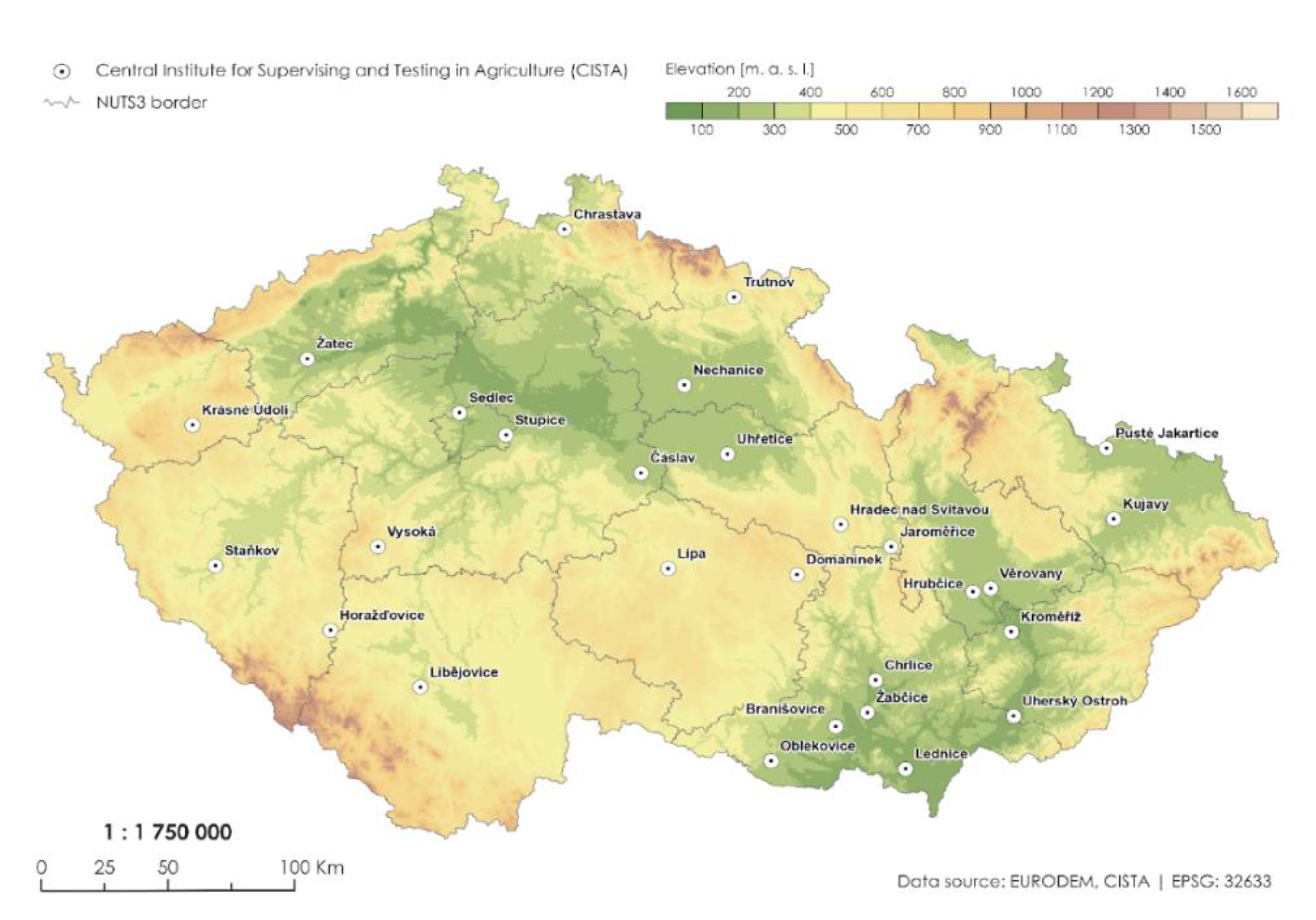
2.1. Stations and Phenological and Meteorological Data
2.2. PhenoClim Model
2.3. Remote Sensing Data
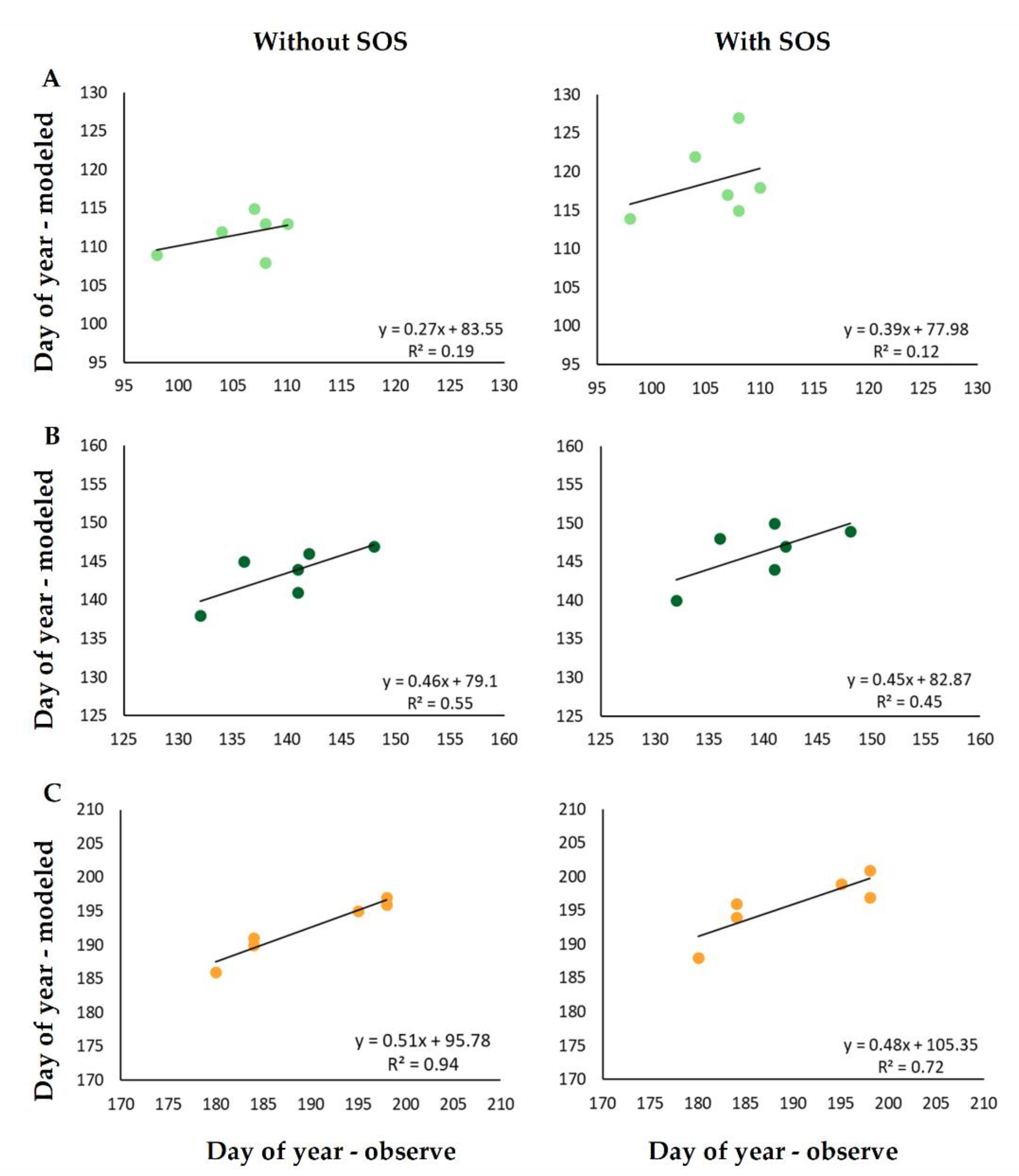
3. Results
4. Discussion
5. Conclusions
Author Contributions
Funding
Institutional Review Board Statement
Informed Consent Statement
Data Availability Statement
Acknowledgments
Conflicts of Interest
Appendix A

| Station | Altitude (m) | Latitude | Longitude | Jointing | Heading | Full Ripeness | |||
|---|---|---|---|---|---|---|---|---|---|
| Period | Years | Period | Years | Period | Years | ||||
| Lednice | 171 | 48°47′59″ | 16°48′12″ | 1994–2021 | 28 | 1976–2021 | 46 | 1976–2021 | 46 |
| Zabcice | 182 | 49°0′41″ | 16°36′9″ | 2000–2021 | 22 | 2000–2021 | 22 | 2000–2021 | 22 |
| Branisovice | 190 | 48°57′46″ | 16°25′54″ | 1995; 2000–2021 | 23 | 1994–1997; 1999–2021 | 27 | 1994–1995; 1999–2021 | 25 |
| Chrlice | 190 | 49°7′52″ | 16°39′9″ | 1994–2021 | 28 | 1961–2021 | 61 | 1961–2021 | 61 |
| Uhersky Ostroh | 196 | 48°59′8″ | 17°23′23 | 1994–2021 | 28 | 1963–1965; 1967–1976; 1978–2021 | 57 | 1963–1965; 1967–2021 | 58 |
| Kromeriz | 201 | 49°17′52″ | 17°23′35″ | 1994–2002; 2004–2005; 2008 | 12 | 1994–1998; 2000–2002; 2004–2005; 2008 | 11 | 1994–1998; 2000–2002; 2004–2005; 2007–2008 | 12 |
| Verovany | 204 | 49°27′39″ | 17°17′16″ | 1994–2021 | 28 | 1970–2021 | 52 | 1970–2021 | 52 |
| Hrubcice | 210 | 49°27′0″ | 17°11′35″ | 1997; 2000–2021 | 23 | 1995–1998; 2000–2021 | 26 | 1997; 2000–2021 | 23 |
| Zatec | 233 | 50°19′37″ | 13°32′44″ | 1993–1997; 1999–2018 | 25 | 1993–1997; 1999–2018 | 25 | 1993–1997; 1999–2018 | 25 |
| Uhretice | 237 | 49°58′44″ | 15°52′2″ | 2000–2021 | 22 | 2000–2021 | 22 | 2000–2021 | 22 |
| Nechanice | 239 | 50°14′14″ | 15°37′57″ | 1992–2021 | 30 | 1992–2021 | 30 | 1992–2021 | 30 |
| Oblekovice | 250 | 48°50′18″ | 16°4′53″ | 1994–2021 | 28 | 1961–1978; 1980–2021 | 60 | 1961–1978; 1980–2021 | 60 |
| Kujavy | 258 | 49°42′11″ | 17°58′21″ | 1992–1998; 2000–2021 | 29 | 1992–1998; 2000–2021 | 29 | 1992–1998; 2000–2021 | 29 |
| Stupice | 277 | 50°3′12″ | 14°38′51″ | 2000–2021 | 22 | 1994–2021 | 28 | 1994–1997; 1999–2021 | 27 |
| Caslav | 290 | 49°54′39″ | 15°23′22″ | 1993–2021 | 29 | 1993–2021 | 29 | 1993–2021 | 29 |
| Puste Jakartice | 295 | 49°58′0″ | 17°56′55″ | 1994–2021 | 28 | 1969–2021 | 53 | 1969–2021 | 53 |
| Sedlec | 300 | 50°8′2″ | 14°23′29″ | 1992–2004 | 13 | 1992–2004 | 13 | 1992–2004 | 13 |
| Chrastava | 345 | 50°49′1″ | 14°58′7″ | 1994–2021 | 28 | 1977–2021 | 45 | 1977–2021 | 45 |
| Stankov | 370 | 49°33′7″ | 13°4′8″ | 1993–2021 | 29 | 1993–2021 | 29 | 1993–2021 | 29 |
| Trutnov | 414 | 50°33′39″ | 15°54′45″ | 1992–1998; 2000–2021 | 29 | 1992–1998; 2000–2021 | 29 | 1992–1998; 2000–2021 | 29 |
| Jaromerice | 425 | 49°37′32″ | 16°45′6″ | 1993–2021 | 29 | 1993–2021 | 29 | 1993–2021 | 29 |
| Libejovice | 434 | 49°6′51″ | 14°11′36″ | 1994–2002; 2004–2011 | 17 | 1961–2002; 2004–2011 | 50 | 1961–2002; 2004–2011 | 50 |
| Horazdovice | 450 | 49°19′14″ | 13°42′3″ | 1994–1998; 2000–2021 | 27 | 1973–1981; 1983–1987; 1989–1992; 1994–1998; 2000–2021 | 45 | 1973–1981; 1983–1987; 1989–1992; 1994–1998; 2000–2021 | 45 |
| Hradec nad Svitavou | 450 | 49°42′41″ | 16°28′50″ | 1992–1998; 2000–2021 | 29 | 1992–1998; 2000–2021 | 29 | 1992–1998; 2000–2021 | 29 |
| Lipa | 505 | 49°33′21″ | 15°32′10″ | 1994–2021 | 28 | 1961–1978; 1980–2021 | 60 | 1961–1978; 1980–1985; 1987–2021 | 59 |
| Domaninek | 570 | 49°31′41″ | 16°14′11″ | 1994–2021 | 28 | 1961–2021 | 61 | 1961–2021 | 61 |
| Vysoka | 590 | 49°38′3″ | 13°57′9″ | 1992–2021 | 30 | 1992–2021 | 30 | 1992–2021 | 30 |
| Krasne Udoli | 647 | 50°4′20″ | 12°55′16″ | 1994; 1996–2002; 2004–2010 | 15 | 1965–1992; 1994; 1996–2000; 2002; 2004–2010 | 42 | 1965–1992; 1994; 1996–2002; 2004–2010 | 43 |
| JOINTING | ||||||||||||||
|---|---|---|---|---|---|---|---|---|---|---|---|---|---|---|
| Station | Model without SOS | Thr 0 | Thr 0.05 | Thr 0.1 | Thr 0.15 | Thr 0.2 | Thr 0.25 | Thr 0.3 | Thr 0.35 | Thr 0.4 | Thr 0.45 | Thr 0.5 | Thr 0.55 | Thr 0.6 |
| RMSE (Days) | RMSE (Days) | RMSE (Days) | RMSE (Days) | RMSE (Days) | RMSE (Days) | RMSE (Days) | RMSE (Days) | RMSE (Days) | RMSE (Days) | RMSE (Days) | RMSE (Days) | RMSE (Days) | RMSE (Days) | |
| Branisovice | 11.3 | 17.7 | 36.3 | 18.7 | 20.9 | 21.1 | 22.7 | 21.9 | 21.9 | 22.2 | 22.4 | 22.7 | 23.2 | 23.2 |
| Caslav | 11.4 | 22.9 | 23.5 | 23.8 | 24.3 | 24.8 | 25.0 | 25.3 | 25.8 | 26.2 | 26.4 | 26.6 | 27.0 | 27.3 |
| Hrubcice | 10.6 | 20.3 | 20.3 | 20.4 | 20.8 | 20.2 | 20.2 | 20.5 | 20.8 | 21.8 | 22.9 | 23.0 | 23.6 | 23.9 |
| Chrlice | 6.9 | 13.2 | 13.4 | 13.6 | 14.0 | 14.7 | 15.2 | 16.4 | 16.7 | 16.8 | 17.6 | 18.8 | 19.4 | 19.6 |
| Oblekovice | 10.2 | 9.7 | 10.0 | 9.6 | 9.9 | 10.3 | 11.5 | 11.5 | 11.9 | 11.9 | 12.2 | 12.8 | 13.0 | 13.1 |
| Puste Jakartice | 10.4 | 15.7 | 15.8 | 15.5 | 16.1 | 16.3 | 16.5 | 16.8 | 17.0 | 17.7 | 18.4 | 18.5 | 18.8 | 19.7 |
| Uhretice | 13.6 | 6.0 | 5.8 | 5.8 | 6.0 | 6.0 | 6.1 | 6.1 | 6.3 | 5.9 | 5.9 | 5.8 | 5.9 | 6.2 |
| Verovany | 6.2 | 11.7 | 12.0 | 12.2 | 12.2 | 12.5 | 12.9 | 13.3 | 13.6 | 13.7 | 14.5 | 15.0 | 15.4 | 15.8 |
| Average | 10.1 | 14.6 | 17.1 | 15.0 | 15.5 | 15.7 | 16.3 | 16.4 | 16.7 | 17.0 | 17.5 | 17.9 | 18.3 | 18.6 |
| HEADING | ||||||||||||||
| Station | model without SOS | Thr 0 | Thr 0.05 | Thr 0.1 | Thr 0.15 | Thr 0.2 | Thr 0.25 | Thr 0.3 | Thr 0.35 | Thr 0.4 | Thr 0.45 | Thr 0.5 | Thr 0.55 | Thr 0.6 |
| RMSE (Days) | RMSE (Days) | RMSE (Days) | RMSE (Days) | RMSE (Days) | RMSE (Days) | RMSE (Days) | RMSE (Days) | RMSE (Days) | RMSE (Days) | RMSE (Days) | RMSE (Days) | RMSE (Days) | RMSE (Days) | |
| Branisovice | 2.4 | 5.0 | 5.0 | 5.0 | 5.6 | 5.8 | 6.0 | 6.0 | 6.0 | 6.2 | 6.2 | 6.5 | 6.5 | 6.7 |
| Caslav | 4.8 | 9.6 | 9.9 | 10.2 | 10.6 | 10.6 | 11.0 | 11.3 | 11.3 | 11.6 | 12.3 | 12.3 | 12.3 | 12.5 |
| Hrubcice | 2.8 | 5.8 | 6.2 | 6.0 | 6.1 | 5.9 | 5.7 | 5.7 | 5.6 | 5.8 | 6.4 | 6.6 | 6.8 | 7.2 |
| Chrlice | 4.9 | 6.1 | 6.1 | 6.5 | 6.5 | 6.7 | 7.1 | 7.5 | 8.1 | 8.1 | 8.3 | 9.2 | 9.6 | 9.7 |
| Oblekovice | 4.9 | 7.9 | 7.9 | 7.6 | 7.8 | 8.1 | 8.6 | 8.7 | 9.1 | 9.1 | 9.1 | 9.5 | 9.5 | 9.7 |
| Puste Jakartice | 5.8 | 8.0 | 8.0 | 8.2 | 8.2 | 8.2 | 8.4 | 8.4 | 8.4 | 8.9 | 9.2 | 9.5 | 9.8 | 10.2 |
| Uhretice | 4.5 | 9.4 | 9.6 | 9.6 | 9.6 | 9.8 | 10.2 | 10.4 | 10.6 | 10.9 | 10.9 | 11.1 | 11.4 | 11.6 |
| Verovany | 5.4 | 10.4 | 10.6 | 10.6 | 10.6 | 10.9 | 10.9 | 11.1 | 11.3 | 11.4 | 11.7 | 12.2 | 12.6 | 12.8 |
| Average | 4.4 | 7.8 | 7.9 | 8.0 | 8.1 | 8.2 | 8.5 | 8.7 | 8.8 | 9.0 | 9.3 | 9.6 | 9.8 | 10.1 |
| FULL RIPENESS | ||||||||||||||
| Station | model without SOS | Thr 0 | Thr 0.05 | Thr 0.1 | Thr 0.15 | Thr 0.2 | Thr 0.25 | Thr 0.3 | Thr 0.35 | Thr 0.4 | Thr 0.45 | Thr 0.5 | Thr 0.55 | Thr 0.6 |
| RMSE (Days) | RMSE (Days) | RMSE (Days) | RMSE (Days) | RMSE (Days) | RMSE (Days) | RMSE (Days) | RMSE (Days) | RMSE (Days) | RMSE (Days) | RMSE (Days) | RMSE (Days) | RMSE (Days) | RMSE (Days) | |
| Branisovice | 7.5 | 10.0 | 10.1 | 10.3 | 11.0 | 11.1 | 11.2 | 11.2 | 11.2 | 11.5 | 11.5 | 11.8 | 11.8 | 11.9 |
| Caslav | 2.8 | 5.7 | 6.4 | 6.4 | 6.6 | 7.1 | 7.3 | 7.3 | 7.9 | 8.1 | 8.4 | 8.3 | 8.6 | 8.7 |
| Hrubcice | 3.4 | 6.4 | 6.4 | 6.1 | 6.3 | 5.8 | 5.6 | 5.6 | 5.5 | 5.5 | 6.0 | 6.1 | 6.1 | 6.3 |
| Chrlice | 4.6 | 4.5 | 4.5 | 4.2 | 4.2 | 4.1 | 4.2 | 3.9 | 3.9 | 3.6 | 3.9 | 4.1 | 4.4 | 4.2 |
| Oblekovice | 9.5 | 9.3 | 9.4 | 9.3 | 9.4 | 9.6 | 9.9 | 9.9 | 10.3 | 10.3 | 10.3 | 10.5 | 10.5 | 10.7 |
| Puste Jakartice | 4.0 | 4.5 | 4.7 | 4.3 | 4.1 | 4.0 | 3.9 | 3.9 | 4.1 | 4.0 | 4.2 | 4.3 | 4.3 | 4.8 |
| Uhretice | 2.3 | 5.7 | 6.0 | 6.0 | 6.2 | 6.2 | 6.2 | 6.2 | 6.4 | 6.2 | 6.0 | 6.4 | 6.4 | 6.5 |
| Verovany | 6.1 | 4.7 | 4.7 | 4.9 | 4.6 | 4.6 | 4.7 | 4.6 | 4.7 | 4.9 | 4.7 | 4.9 | 5.2 | 5.4 |
| Average | 5.0 | 6.4 | 6.5 | 6.4 | 6.6 | 6.6 | 6.6 | 6.6 | 6.7 | 6.8 | 6.9 | 7.1 | 7.2 | 7.3 |
| JOINTING | ||||||||||||||
|---|---|---|---|---|---|---|---|---|---|---|---|---|---|---|
| Station | Model without SOS | Thr 0 | Thr 0.05 | Thr 0.1 | Thr 0.15 | Thr 0.2 | Thr 0.25 | Thr 0.3 | Thr 0.35 | Thr 0.4 | Thr 0.45 | Thr 0.5 | Thr 0.55 | Thr 0.6 |
| RMSE (Days) | RMSE (Days) | RMSE (Days) | RMSE (Days) | RMSE (Days) | RMSE (Days) | RMSE (Days) | RMSE (Days) | RMSE (Days) | RMSE (Days) | RMSE (Days) | RMSE (Days) | RMSE (Days) | RMSE (Days) | |
| Branisovice | 11.3 | 17.7 | 36.3 | 18.7 | 20.9 | 20.9 | 21.1 | 21.9 | 21.9 | 22.2 | 22.4 | 22.7 | 23.2 | 23.2 |
| Caslav | 11.4 | 22.9 | 23.4 | 23.8 | 24.3 | 24.8 | 25.0 | 25.3 | 25.8 | 26.2 | 26.4 | 26.6 | 27.0 | 27.3 |
| Hrubcice | 10.6 | 21.5 | 21.8 | 22.0 | 22.5 | 22.4 | 22.8 | 23.4 | 23.8 | 23.9 | 24.6 | 24.7 | 25.0 | 25.4 |
| Chrlice | 6.9 | 15.4 | 16.2 | 16.2 | 16.8 | 17.0 | 17.1 | 17.8 | 18.3 | 18.6 | 19.4 | 20.0 | 20.3 | 20.3 |
| Oblekovice | 10.2 | 11.0 | 11.0 | 12.0 | 12.4 | 12.6 | 12.9 | 12.9 | 13.1 | 13.6 | 13.8 | 14.5 | 15.1 | 15.2 |
| Puste Jakartice | 10.4 | 15.7 | 15.8 | 15.5 | 16.1 | 16.3 | 16.5 | 16.8 | 17.0 | 18.0 | 18.4 | 18.5 | 18.8 | 19.7 |
| Uhretice | 13.6 | 5.2 | 5.0 | 5.2 | 5.3 | 5.2 | 5.3 | 5.6 | 5.9 | 6.2 | 6.4 | 6.4 | 6.8 | 6.8 |
| Verovany | 6.2 | 12.5 | 12.5 | 12.9 | 13.1 | 13.5 | 13.8 | 14.3 | 14.5 | 15.3 | 16.2 | 16.8 | 16.9 | 17.4 |
| Average | 10.1 | 15.2 | 17.8 | 15.8 | 16.4 | 16.6 | 16.8 | 17.2 | 17.6 | 18.0 | 18.5 | 18.8 | 19.1 | 19.4 |
| HEADING | ||||||||||||||
| Station | Model without SOS | Thr 0 | Thr 0.05 | Thr 0.1 | Thr 0.15 | Thr 0.2 | Thr 0.25 | Thr 0.3 | Thr 0.35 | Thr 0.4 | Thr 0.45 | Thr 0.5 | Thr 0.55 | Thr 0.6 |
| RMSE (Days) | RMSE (Days) | RMSE (Days) | RMSE (Days) | RMSE (Days) | RMSE (Days) | RMSE (Days) | RMSE (Days) | RMSE (Days) | RMSE (Days) | RMSE (Days) | RMSE (Days) | RMSE (Days) | RMSE (Days) | |
| Branisovice | 2.4 | 5.0 | 5.0 | 5.0 | 5.6 | 5.8 | 6.0 | 6.0 | 6.0 | 6.2 | 6.2 | 6.5 | 6.5 | 6.7 |
| Caslav | 4.8 | 9.6 | 9.9 | 10.2 | 10.6 | 10.6 | 11.0 | 11.3 | 11.3 | 11.6 | 12.3 | 12.3 | 12.3 | 12.5 |
| Hrubcice | 2.8 | 6.2 | 6.5 | 6.6 | 6.6 | 6.5 | 6.7 | 6.7 | 7.2 | 7.4 | 7.7 | 7.7 | 7.9 | 8.1 |
| Chrlice | 4.9 | 7.0 | 7.1 | 7.5 | 7.9 | 8.2 | 8.2 | 8.5 | 8.7 | 9.0 | 9.6 | 10.1 | 10.4 | 10.4 |
| Oblekovice | 4.9 | 7.9 | 7.9 | 8.7 | 8.9 | 9.1 | 9.5 | 9.5 | 9.5 | 9.8 | 9.8 | 10.3 | 10.7 | 11.0 |
| Puste Jakartice | 5.8 | 8.0 | 8.0 | 8.2 | 8.2 | 8.2 | 8.4 | 8.4 | 8.4 | 9.1 | 9.2 | 9.5 | 9.8 | 10.2 |
| Uhretice | 4.5 | 8.7 | 9.6 | 9.6 | 9.7 | 10.0 | 10.4 | 10.7 | 10.7 | 11.1 | 11.5 | 11.5 | 12.0 | 12.2 |
| Verovany | 5.4 | 10.7 | 10.7 | 10.9 | 10.9 | 11.3 | 11.5 | 11.5 | 12.0 | 12.5 | 12.9 | 13.6 | 13.6 | 14.0 |
| Average | 4.4 | 7.9 | 8.1 | 8.3 | 8.6 | 8.7 | 8.9 | 9.1 | 9.3 | 9.6 | 9.9 | 10.2 | 10.4 | 10.6 |
| FULL RIPENESS | ||||||||||||||
| Station | Model without SOS | Thr 0 | Thr 0.05 | Thr 0.1 | Thr 0.15 | Thr 0.2 | Thr 0.25 | Thr 0.3 | Thr 0.35 | Thr 0.4 | Thr 0.45 | Thr 0.5 | Thr 0.55 | Thr 0.6 |
| RMSE (Days) | RMSE (Days) | RMSE (Days) | RMSE (Days) | RMSE (Days) | RMSE (Days) | RMSE (Days) | RMSE (Days) | RMSE (Days) | RMSE (Days) | RMSE (Days) | RMSE (Days) | RMSE (Days) | RMSE (Days) | |
| Branisovice | 7.5 | 10.0 | 10.1 | 10.3 | 11.0 | 11.1 | 11.2 | 11.2 | 11.2 | 11.5 | 11.5 | 11.8 | 11.8 | 11.9 |
| Caslav | 2.8 | 5.7 | 6.4 | 6.4 | 6.6 | 7.1 | 7.3 | 7.3 | 7.9 | 8.1 | 8.4 | 8.3 | 8.6 | 8.7 |
| Hrubcice | 3.4 | 6.2 | 6.0 | 6.3 | 6.6 | 6.3 | 6.4 | 6.3 | 6.8 | 6.8 | 6.8 | 7.0 | 7.4 | 7.5 |
| Chrlice | 4.6 | 3.8 | 3.9 | 3.8 | 3.8 | 3.9 | 3.6 | 3.7 | 3.7 | 4.0 | 4.2 | 4.4 | 4.4 | 4.6 |
| Oblekovice | 9.5 | 9.6 | 9.6 | 10.1 | 10.2 | 10.4 | 10.4 | 10.4 | 10.5 | 10.9 | 10.9 | 11.4 | 11.9 | 12.1 |
| Puste Jakartice | 4.0 | 4.5 | 4.7 | 4.3 | 4.1 | 4.0 | 3.9 | 3.9 | 4.1 | 4.0 | 4.3 | 4.3 | 4.3 | 4.8 |
| Uhretice | 2.3 | 5.0 | 5.3 | 5.3 | 5.3 | 5.5 | 5.6 | 6.1 | 6.1 | 6.1 | 6.5 | 6.5 | 6.9 | 6.9 |
| Verovany | 6.1 | 4.4 | 4.4 | 4.4 | 4.6 | 4.4 | 4.6 | 4.7 | 4.9 | 5.6 | 5.6 | 6.2 | 6.4 | 6.4 |
| Average | 5.0 | 6.2 | 6.3 | 6.3 | 6.5 | 6.6 | 6.6 | 6.7 | 6.9 | 7.1 | 7.3 | 7.5 | 7.7 | 7.9 |
References
- Sujetoviene, G.; Velica, R.; Kanapickas, A.; Kriauciuniene, Z.; Romanovskaja, D.; Baksiene, E.; Vaguseviciene, I.; Klepeckas, M.; Juknys, R. Climate-change-related long-term historical and projected changes to spring barley phenological development in Lithuania. J. Agric. Sci. 2018, 156, 1061–1069. [Google Scholar] [CrossRef]
- Fu, Y.S.; Li, X.X.; Zhou, X.C.; Geng, X.J.; Guo, Y.H.; Zhang, Y.R. Progress in plant phenology modeling under global climate change. Sci. China-Earth Sci. 2020, 63, 1237–1247. [Google Scholar] [CrossRef]
- Xiao, L.J.; Liu, B.; Zhang, H.X.; Gu, J.Y.; Fu, T.Y.; Asseng, S.; Liu, L.L.; Tang, L.; Cao, W.X.; Zhu, Y. Modeling the response of winter wheat phenology to low temperature stress at elongation and booting stages. Agric. For. Meteorol. 2021, 303, 13. [Google Scholar] [CrossRef]
- Oteros, J.; Garcia-Mozo, H.; Botey, R.; Mestre, A.; Galan, C. Variations in cereal crop phenology in Spain over the last twenty-six years (1986–2012). Clim. Chang. 2015, 130, 545–558. [Google Scholar] [CrossRef]
- Porter, J.R.; Gawith, M. Temperatures and the growth and development of wheat: A review. Eur. J. Agron. 1999, 10, 23–36. [Google Scholar] [CrossRef]
- Salazar-Gutierrez, M.R.; Johnson, J.; Chaves-Cordoba, B.; Hoogenboom, G. Relationship of base temperature to development of winter wheat. Int. J. Plant Prod. 2013, 7, 741–762. [Google Scholar]
- Zhou, M.; Ma, X.; Wang, K.K.; Cheng, T.; Tian, Y.C.; Wang, J.; Zhu, Y.; Hu, Y.Q.; Niu, Q.S.; Gui, L.J.; et al. Detection of phenology using an improved shape model on time-series vegetation index in wheat. Comput. Electron. Agric. 2020, 173, 13. [Google Scholar] [CrossRef]
- Zhao, F.; Yang, G.J.; Yang, X.D.; Cen, H.Y.; Zhu, Y.H.; Han, S.Y.; Yang, H.; He, Y.; Zhao, C.J. Determination of Key Phenological Phases of Winter Wheat Based on the Time-Weighted Dynamic Time Warping Algorithm and MODIS Time-Series Data. Remote Sens. 2021, 13, 1836. [Google Scholar] [CrossRef]
- Kostková, M.; Hlavinka, P.; Pohanková, E.; Kersebaum, K.C.; Nendel, C.; Gobin, A.; Olesen, J.E.; Ferrise, R.; Dibari, C.; Takac, J.; et al. Performance of 13 crop simulation models and their ensemble for simulating four field crops in Central Europe. J. Agric. Sci. 2021, 159, 69–89. [Google Scholar] [CrossRef]
- Černá, H.; Bartošová, L.; Trnka, M.; Bauer, Z.; Štěpánek, P.; Možný, M.; Dubrovský, M.; Žalud, Z. The analysis of long-term phenological data of apricot tree (Prunus armeniaca L.) in southern Moravia during 1927–2009. Acta Univ. Agric. Silvic. Mendel. Brun. 2012, 60, 9–18. [Google Scholar] [CrossRef]
- Marcinkowski, P.; Piniewski, M. Effect of climate change on sowing and harvest dates of spring barley and maize in Poland. Int. Agrophys. 2018, 32, 265–271. [Google Scholar] [CrossRef]
- Bhutto, S.A.; Wang, X.Y.; Wang, J. The start and end of the growing season in Pakistan during 1982–2015. Environ. Earth Sci. 2019, 78, 10. [Google Scholar] [CrossRef]
- Song, Y.; Wang, J.; Yu, Q.; Huang, J.X. Using MODIS LAI Data to Monitor Spatio-Temporal Changes of Winter Wheat Phenology in Response to Climate Warming. Remote Sens. 2020, 12, 786. [Google Scholar] [CrossRef] [Green Version]
- Steele-Dunne, S.C.; McNairn, H.; Monsivais-Huertero, A.; Judge, J.; Liu, P.W.; Papathanassiou, K. Radar Remote Sensing of Agricultural Canopies: A Review. IEEE J. Sel. Top. Appl. Earth Obs. Remote Sens. 2017, 10, 2249–2273. [Google Scholar] [CrossRef] [Green Version]
- Mercier, A.; Betbeder, J.; Baudry, J.; Le Roux, V.; Spicher, F.; Lacoux, J.; Roger, D.; Hubert-Moy, L. Evaluation of Sentinel-1 & 2 time series for predicting wheat and rapeseed phenological stages. ISPRS J. Photogramm. Remote Sens. 2020, 163, 231–256. [Google Scholar] [CrossRef]
- Caparros-Santiago, J.A.; Rodriguez-Galiano, V.; Dash, J. Land surface phenology as indicator of global terrestrial ecosystem dynamics: A systematic review. ISPRS J. Photogramm. Remote Sens. 2021, 171, 330–347. [Google Scholar] [CrossRef]
- Menzel, A.; Yuan, Y.; Matiu, M.; Sparks, T.; Scheifinger, H.; Gehrig, R.; Estrella, N. Climate change fingerprints in recent European plant phenology. Glob. Chang. Biol. 2020, 26, 2599–2612. [Google Scholar] [CrossRef] [PubMed] [Green Version]
- Parmesan, C.; Yohe, G. A globally coherent fingerprint of climate change impacts across natural systems. Nature 2003, 421, 37–42. [Google Scholar] [CrossRef]
- Buntgen, U.; Piermattei, A.; Krusic, P.J.; Esper, J.; Sparks, T.; Crivellaro, A. Plants in the UK flower a month earlier under recent warming. Proc. R. Soc. B-Biol. Sci. 2022, 289, 9. [Google Scholar] [CrossRef]
- Bartošová, L.; Dížková, P.; Bauerová, J.; Hájková, L.; Fischer, M.; Balek, J.; Bláhová, M.; Možný, M.; Zahradníček, P.; Štěpánek, P.; et al. Phenological Response of Flood Plain Forest Ecosystem Species to Climate Change during 1961–2021. Atmosphere 2022, 13, 978. [Google Scholar] [CrossRef]
- Hájková, L.; Možný, M.; Oušková, V.; Bartošová, L.; Dížková, P.; Žalud, Z. Meteorological Variables That Affect the Beginning of Flowering of the Winter Oilseed Rape in the Czech Republic. Atmosphere 2021, 12, 1444. [Google Scholar] [CrossRef]
- Rezaei, E.E.; Siebert, S.; Ewert, F. Climate and management interaction cause diverse crop phenology trends. Agric. For. Meteorol. 2017, 233, 55–70. [Google Scholar] [CrossRef]
- Bai, H.Z.; Xiao, D.P.; Zhang, H.; Tao, F.L.; Hu, Y.H. Impact of warming climate, sowing date, and cultivar shift on rice phenology across China during 1981–2010. Int. J. Biometeorol. 2019, 63, 1077–1089. [Google Scholar] [CrossRef]
- Huang, X.; Zhu, W.Q.; Wang, X.Y.; Zhan, P.; Liu, Q.F.; Li, X.Y.; Sun, L.X. A Method for Monitoring and Forecasting the Heading and Flowering Dates of Winter Wheat Combining Satellite-Derived Green-up Dates and Accumulated Temperature. Remote Sens. 2020, 12, 3536. [Google Scholar] [CrossRef]
- Zhao, F.; Yang, G.J.; Yang, H.; Long, H.L.; Xu, W.M.; Zhu, Y.H.; Meng, Y.; Han, S.Y.; Liu, M. A Method for Prediction of Winter Wheat Maturity Date Based on MODIS Time Series and Accumulated Temperature. Agriculture 2022, 12, 945. [Google Scholar] [CrossRef]
- R Core Team. R: A Language and Environment for Statistical Computing; R Foundation for Statistical Computing: Vienna, Austria, 2019; Available online: https://www.R-project.org/ (accessed on 8 October 2022).
- Štěpánek, P. AnClim—Software for Time Series Analysis; Department of Geography, Faculty of Natural Sciences, Masaryk University: Brno, Czech Republic, 2008. [Google Scholar]
- Štěpánek, P.; Zahradníček, P.; Brázdil, R.; Tolasz, R. Metodologie Kontroly a Homogenizace Časových řad v Klimatologii; ČHMÚ: Prague, Czechia, 2012; 118p, ISBN 978-80-86690-97-1. [Google Scholar]
- Štěpánek, P.; Zahradníček, P.; Huth, R. Interpolation techniques used for data quality control and calculation of technical series: An example of a Central European daily time series. Időjárás 2011, 115, 87–98. [Google Scholar]
- Štěpánek, P.; Zahradníček, P.; Farda, A. Experiences with data quality control and homogenization of daily records of various meteorological elements in the Czech Republic in the period 1961–2010. Időjárás 2013, 117, 123–141. [Google Scholar]
- Squintu, A.A.; van der Schrier, G.; Štěpánek, P.; Zahradníček, P.; Tank, A.K. Comparison of homogenization methods for daily temperature series against an observation-based benchmark dataset. Theor. Appl. Climatol. 2020, 140, 285–301. [Google Scholar] [CrossRef] [Green Version]
- Bartošová, L.; Bauer, Z.; Trnka, M.; Štěpánek, P.; Žalud, Z. Climatic factors and their influence on onset and duration of phenological phases of chosen plants at locations south Moravia during 1961–2007. Acta Univ. Agric. Silvic. Mendel. Brun. 2010, 58, 35–44. [Google Scholar] [CrossRef] [Green Version]
- Trnka, M.; Rötter, R.P.; Ruiz-Ramos, M.; Kersebaum, K.C.; Olesen, J.E.; Žalud, Z.; Semenov, M.A. Adverse weather conditions for European wheat production will become more frequent with climate change. Nat. Clim. Chang. 2014, 4, 637–643. [Google Scholar] [CrossRef]
- Trnka, M.; Kocmankova, E.; Balek, J.; Eitzinger, J.; Ruget, F.; Formayer, H.; Hlavinka, P.; Schaumberger, A.; Horakova, V.; Možný, M.; et al. Simple snow cover model for agrometeorological applications. Agric. For. Meteorol. 2010, 150, 1115–1127. [Google Scholar] [CrossRef]
- Vermote, E.; Wolfe, R. MOD09GQ MODIS/Terra Surface Reflectance Daily L2G Global 250 m SIN Grid V006 [Data Set]; NASA EOSDIS Land Processes DAAC; United States Geological Survey: Reston, VA, USA, 2015. [Google Scholar] [CrossRef]
- Zeng, L.L.; Wardlow, B.D.; Xiang, D.X.; Hu, S.; Li, D.R. A review of vegetation phenological metrics extraction using time-series, multispectral satellite data. Remote Sens. Environ. 2020, 237, 20. [Google Scholar] [CrossRef]
- Xiao, D.P.; Tao, F.L.; Liu, Y.J.; Shi, W.J.; Wang, M.; Liu, F.S.; Zhang, S.; Zhu, Z. Observed changes in winter wheat phenology in the North China Plain for 1981–2009. Int. J. Biometeorol. 2013, 57, 275–285. [Google Scholar] [CrossRef]
- Hu, Q.; Weiss, A.; Feng, S.; Baenziger, P.S. Earlier winter wheat heading dates and warmer spring in the US Great Plains. Agric. For. Meteorol. 2005, 135, 284–290. [Google Scholar] [CrossRef]
- Siebert, S.; Ewert, F. Spatio-temporal patterns of phenological development in Germany in relation to temperature and day length. Agric. For. Meteorol. 2012, 152, 44–57. [Google Scholar] [CrossRef]
- Xiao, D.P.; Qi, Y.Q.; Li, Z.Q.; Wang, R.D.; Moiwo, J.P.; Liu, F.S. Impact of thermal time shift on wheat phenology and yield under warming climate in the Huang-Huai-Hai Plain, China. Front. Earth Sci. 2017, 11, 148–155. [Google Scholar] [CrossRef]
- Liu, Y.J.; Chen, Q.M.; Ge, Q.S.; Dai, J.H.; Dou, Y. Effects of climate change and agronomic practice on changes in wheat phenology. Clim. Chang. 2018, 150, 273–287. [Google Scholar] [CrossRef]
- Eitzinger, J.; Trnka, M.; Semeradová, D.; Thaler, S.; Svobodová, E.; Hlavinka, P.; Siska, B.; Takac, J.; Malatinska, L.; Nováková, M.; et al. Regional climate change impacts on agricultural crop production in Central and Eastern Europe—Hotspots, regional differences and common trends. J. Agric. Sci. 2013, 151, 787–812. [Google Scholar] [CrossRef]
- Pullens, J.W.M.; Sorensen, C.A.G.; Olesen, J.E. Temperature-based prediction of harvest date in winter and spring cereals as a basis for assessing viability for growing cover crops. Field Crop. Res. 2021, 264, 11. [Google Scholar] [CrossRef]


| Station | Altitude (m) | Latitude | Longitude | Jointing | Heading | Full Ripeness |
|---|---|---|---|---|---|---|
| Years | Years | Years | ||||
| Lednice | 171 | 48°47′59″ | 16°48′12″ | 28 | 46 | 46 |
| Zabcice | 182 | 49°0′41″ | 16°36′9″ | 22 | 22 | 22 |
| Branisovice | 190 | 48°57′46″ | 16°25′54″ | 23 | 27 | 25 |
| Chrlice | 190 | 49°7′52″ | 16°39′9″ | 28 | 61 | 61 |
| Uhersky Ostroh | 196 | 48°59′8″ | 17°23′23″ | 28 | 57 | 58 |
| Kromeriz | 201 | 49°17′52″ | 17°23′35″ | 12 | 11 | 12 |
| Verovany | 204 | 49°27′39″ | 17°17′16″ | 28 | 52 | 52 |
| Hrubcice | 210 | 49°27′0″ | 17°11′35″ | 23 | 26 | 23 |
| Zatec | 233 | 50°19′37″ | 13°32′44″ | 25 | 25 | 25 |
| Uhretice | 237 | 49°58′44″ | 15°52′2″ | 22 | 22 | 22 |
| Nechanice | 239 | 50°14′14″ | 15°37′57″ | 30 | 30 | 30 |
| Oblekovice | 250 | 48°50′18″ | 16°4′53″ | 28 | 60 | 60 |
| Kujavy | 258 | 49°42′11″ | 17°58′21″ | 29 | 29 | 29 |
| Stupice | 277 | 50°3′12″ | 14°38′51″ | 22 | 28 | 27 |
| Caslav | 290 | 49°54′39″ | 15°23′22″ | 29 | 29 | 29 |
| Puste Jakartice | 295 | 49°58′0″ | 17°56′55″ | 28 | 53 | 53 |
| Sedlec | 300 | 50°8′2″ | 14°23′29″ | 13 | 13 | 13 |
| Chrastava | 345 | 50°49′1″ | 14°58′7″ | 28 | 45 | 45 |
| Stankov | 370 | 49°33′7″ | 13°4′8″ | 29 | 29 | 29 |
| Trutnov | 414 | 50°33′39″ | 15°54′45″ | 29 | 29 | 29 |
| Jaromerice | 425 | 49°37′32″ | 16°45′6″ | 29 | 29 | 29 |
| Libejovice | 434 | 49°6′51″ | 14°11′36″ | 17 | 50 | 50 |
| Horazdovice | 450 | 49°19′14″ | 13°42′3″ | 27 | 45 | 45 |
| Hradec nad Svitavou | 450 | 49°42′41″ | 16°28′50″ | 29 | 29 | 29 |
| Lipa | 505 | 49°33′21″ | 15°32′10″ | 28 | 60 | 59 |
| Domaninek | 570 | 49°31′41″ | 16°14′11″ | 28 | 61 | 61 |
| Vysoka | 590 | 49°38′3″ | 13°57′9″ | 30 | 30 | 30 |
| Krasne Udoli | 647 | 50°4′20″ | 12°55′16″ | 15 | 42 | 43 |
| JOINTING | HEADING | FULL RIPENESS | ||||||||
|---|---|---|---|---|---|---|---|---|---|---|
| Stations | Altitude (m) | Trend/10 Years/Days | In Situ/Modeled R2 | Correlation/ Modeled r | Trend/10 Years/Days | In Situ/Modeled R2 | Correlation/ Modeled r | Trend/10 Years/Days | In Situ/Modeled R2 | Correlation/ Modeled r |
| Lednice | 171 | −3.9 | 0.44 | 0.67 | −3.2 *** | 0.75 | 0.87 | −3.8 *** | 0.52 | 0.72 |
| Zabcice | 182 | −1.2 | 0.53 | 0.73 | 2 | 0.65 | 0.81 | −1.1 | 0.80 | 0.90 |
| Branisovice | 190 | −2.5 | 0.64 | 0.80 | −1.3 | 0.69 | 0.83 | −2.7 | 0.75 | 0.87 |
| Chrlice | 190 | −2.7 | 0.63 | 0.79 | −3.3 *** | 0.74 | 0.86 | −3.0 *** | 0.81 | 0.90 |
| Uhersky Ostroh | 196 | −6.0 ** | 0.61 | 0.78 | −4.1 *** | 0.71 | 0.84 | −2.2 ** | 0.47 | 0.68 |
| Kromeriz | 201 | −1.9 | 0.33 | 0.57 | 0.4 | 0.91 | 0.96 | 0.3 | 0.79 | 0.89 |
| Verovany | 204 | −4.1 * | 0.67 | 0.82 | −3.2 *** | 0.73 | 0.85 | −4.4 *** | 0.79 | 0.89 |
| Hrubcice | 210 | −1.1 | 0.60 | 0.78 | −1.8 | 0.77 | 0.88 | −0.7 | 0.59 | 0.77 |
| Zatec | 233 | −4.6 * | 0.66 | 0.81 | −1.8 | 0.83 | 0.91 | −2.6 | 0.69 | 0.83 |
| Uhretice | 237 | −3.7 | 0.23 | 0.48 | 2.7 | 0.64 | 0.80 | −2 | 0.71 | 0.84 |
| Nechanice | 239 | −1.7 | 0.55 | 0.74 | −2.4 | 0.77 | 0.88 | −5.0 ** | 0.49 | 0.70 |
| Oblekovice | 250 | −4.5 * | 0.59 | 0.77 | −3.5 *** | 0.63 | 0.79 | −3.7 *** | 0.75 | 0.87 |
| Kujavy | 258 | −3.5* | 0.60 | 0.78 | −3.5* | 0.58 | 0.76 | −4.7** | 0.58 | 0.76 |
| Stupice | 277 | −1.2 | 0.60 | 0.77 | −2.3 | 0.74 | 0.86 | −5.9 *** | 0.76 | 0.87 |
| Caslav | 290 | −1.7 | 0.38 | 0.62 | −1.4 | 0.65 | 0.81 | −2.3 | 0.79 | 0.89 |
| Puste Jakartice | 295 | −5.5 ** | 0.66 | 0.82 | −2.57 *** | 0.64 | 0.80 | −4.2 *** | 0.88 | 0.94 |
| Sedlec | 300 | −9.2 * | 0.44 | 0.67 | −2.8 | 0.87 | 0.93 | −3.3 | 0.86 | 0.93 |
| Chrastava | 345 | −6.9 ** | 0.44 | 0.66 | −3.0 *** | 0.82 | 0.90 | −5.2 *** | 0.86 | 0.93 |
| Stankov | 370 | −2.8 | 0.45 | 0.67 | −0.8 | 0.77 | 0.88 | −5.3 ** | 0.63 | 0.79 |
| Trutnov | 414 | −1 | 0.47 | 0.68 | −1.5 | 0.75 | 0.87 | −5.7 ** | 0.54 | 0.73 |
| Jaromerice | 425 | −0.04 | 0.20 | 0.45 | −0.3 | 0.78 | 0.88 | −3 | 0.73 | 0.85 |
| Libejovice | 434 | −1.6 | 0.76 | 0.87 | −3.4 *** | 0.87 | 0.93 | −0.9 | 0.60 | 0.77 |
| Horazdovice | 450 | −0.7 | 0.45 | 0.67 | −4.1 *** | 0.76 | 0.87 | −4.6 *** | 0.67 | 0.82 |
| Hradec n. Svitavou | 450 | −3.2 | 0.58 | 0.76 | −2 | 0.82 | 0.91 | −3.2 * | 0.79 | 0.89 |
| Lipa | 505 | −5.3 ** | 0.58 | 0.76 | −4.2 *** | 0.80 | 0.90 | −3.4 *** | 0.76 | 0.87 |
| Domaninek | 570 | −5.9 ** | 0.58 | 0.76 | −3.6 *** | 0.73 | 0.86 | −3.4 *** | 0.70 | 0.84 |
| Vysoka | 590 | −5.9 *** | 0.60 | 0.78 | −1.4 | 0.86 | 0.93 | −3.1 * | 0.78 | 0.88 |
| Krasne Udoli | 647 | −4 | 0.40 | 0.63 | −3.6 *** | 0.77 | 0.88 | −3.6 ** | 0.79 | 0.89 |
| Best Predictor (Tmax)—Average of 10 Models | ||||||
|---|---|---|---|---|---|---|
| Phenological Phase | RMSE | Tbase | Standard Deviation of Tbase | GDD | R2 | r |
| Jointing | 9.4 | 2.2 | 1.1 | 284.6 | 0.60 | 0.77 |
| Heading | 4.3 | 4.7 | 0.4 | 493.3 | 0.75 | 0.87 |
| Full ripeness | 5.3 | 4.7 | 0.5 | 1207.9 | 0.82 | 0.90 |
| VI | Model without SOS | Thr 0 | Thr 0.05 | Thr 0.1 | Thr 0.15 | Thr 0.2 | Thr 0.25 | Thr 0.3 | Thr 0.35 | Thr 0.4 | Thr 0.45 | Thr 0.5 | Thr 0.55 | Thr 0.6 |
|---|---|---|---|---|---|---|---|---|---|---|---|---|---|---|
| RMSE (Days) | RMSE (Days) | RMSE (Days) | RMSE (Days) | RMSE (Days) | RMSE (Days) | RMSE (Days) | RMSE (Days) | RMSE (Days) | RMSE (Days) | RMSE (Days) | RMSE (Days) | RMSE (Days) | RMSE (Days) | |
| JOINTING | ||||||||||||||
| NDVI | 10.1 | 14.6 | 17.1 | 15.0 | 15.5 | 15.7 | 16.3 | 16.4 | 16.7 | 17.0 | 17.5 | 17.9 | 18.3 | 18.6 |
| EVI2 | 10.1 | 15.2 | 17.8 | 15.8 | 16.4 | 16.6 | 16.8 | 17.2 | 17.6 | 18.0 | 18.5 | 18.8 | 19.1 | 19.4 |
| HEADING | ||||||||||||||
| NDVI | 4.4 | 7.8 | 7.9 | 8.0 | 8.1 | 8.2 | 8.5 | 8.7 | 8.8 | 9.0 | 9.3 | 9.6 | 9.8 | 10.1 |
| EVI2 | 4.4 | 7.9 | 8.1 | 8.3 | 8.6 | 8.7 | 8.9 | 9.1 | 9.3 | 9.6 | 9.9 | 10.2 | 10.4 | 10.6 |
| FULL RIPENESS | ||||||||||||||
| NDVI | 5.0 | 6.4 | 6.5 | 6.4 | 6.6 | 6.6 | 6.6 | 6.6 | 6.7 | 6.8 | 6.9 | 7.1 | 7.2 | 7.3 |
| EVI2 | 5.0 | 6.2 | 6.3 | 6.3 | 6.5 | 6.6 | 6.6 | 6.7 | 6.9 | 7.1 | 7.3 | 7.5 | 7.7 | 7.9 |
Publisher’s Note: MDPI stays neutral with regard to jurisdictional claims in published maps and institutional affiliations. |
© 2022 by the authors. Licensee MDPI, Basel, Switzerland. This article is an open access article distributed under the terms and conditions of the Creative Commons Attribution (CC BY) license (https://creativecommons.org/licenses/by/4.0/).
Share and Cite
Dížková, P.; Bartošová, L.; Bláhová, M.; Balek, J.; Hájková, L.; Semerádová, D.; Bohuslav, J.; Pohanková, E.; Žalud, Z.; Trnka, M. Modeling Phenological Phases of Winter Wheat Based on Temperature and the Start of the Growing Season. Atmosphere 2022, 13, 1854. https://doi.org/10.3390/atmos13111854
Dížková P, Bartošová L, Bláhová M, Balek J, Hájková L, Semerádová D, Bohuslav J, Pohanková E, Žalud Z, Trnka M. Modeling Phenological Phases of Winter Wheat Based on Temperature and the Start of the Growing Season. Atmosphere. 2022; 13(11):1854. https://doi.org/10.3390/atmos13111854
Chicago/Turabian StyleDížková, Petra, Lenka Bartošová, Monika Bláhová, Jan Balek, Lenka Hájková, Daniela Semerádová, Jakub Bohuslav, Eva Pohanková, Zdeněk Žalud, and Miroslav Trnka. 2022. "Modeling Phenological Phases of Winter Wheat Based on Temperature and the Start of the Growing Season" Atmosphere 13, no. 11: 1854. https://doi.org/10.3390/atmos13111854