1. Introduction
With the development of the economy and society and the improvement in living standards, the number of motor vehicles in China has increased dramatically. In 2020, the total number of motor vehicles in China reached 372 million [
1]. The pollution problem caused by motor vehicles is a growing concern [
2]. Previously, national regulations around the world required emission tests for light-duty vehicles to be conducted on laboratory drums in specific cycles [
3]. However, numerous studies [
4,
5,
6,
7,
8,
9] have shown that a single test cycle cannot fully cover the actual driving conditions. The results of laboratory and actual driving emission (RDE) tests may differ significantly. In 2022, China will fully implement the China VI emission standard for light-duty vehicles [
10]. Compared with the previous emissions standard, the new standard reflects the RDE concerning the Euro 6 standard [
11] and combines with China’s national conditions. It requires using Portable Emission Measure System (PEMS) equipment to evaluate the actual vehicle emissions on the road.
In the RDE test, the on-road emissions results are affected by road traffic conditions, vehicle type, and driver driving behavior [
12]. The test should cover all road conditions, including urban, suburban, and high-speed [
13]. In addition, the test vehicle should be in a normal driving style, normal driving conditions, and load on paved roads. The influencing factors include terrain, quality of the road surface, road width, traffic flow, number of traffic lights, traffic management, weather, wind speed, temperature and humidity, and the degree of aggressive driving behavior [
14]. According to the research data sheet developed by the Ministry of Ecology and Environment for China VI emission standard for light-duty vehicles, the acceleration process of vehicles in China is much more moderate than that in the United States and most European countries, and the average load of vehicles while driving is lower [
15]. The actual road traffic conditions and driving behavior in China significantly impact the RDE test process and data processing [
16]. However, there are significant traffic risks in conducting RDE tests with regard to Chinese road conditions and poor test stability, especially for PN tests [
17,
18], which often cause RDE tests to exceed the limit due to driving behavior, vehicle type, road conditions, etc. [
19,
20]. Therefore, more ways are needed to assist in the running of the RDE test.
The machine learning model is expected to assist in RDE testing as a method that does not require physical knowledge [
21,
22,
23]. Zhang et al. [
24] developed a CO
2 emission model based on a long and short-term memory neural network (NN) with data measured using PEMS. The results showed that vehicle speed, acceleration, vehicle specific power (VSP), and road slope significantly affect the instantaneous CO
2 emission rate. Jaikumar et al. [
25] developed real-time exhaust emissions of passenger cars based on NN. The vehicle characteristics, such as revolutions per minute, speed, acceleration, and VSP were used as input to the model. Hien et al. [
26] developed a prediction model to analyze the fuel consumption and CO
2 emission of light-duty vehicles based on convolutional NN. Seo et al. [
27] combined a vehicle dynamics model with an NN model, to calculate CO
2, NOx, and THC emissions. They also used RDE test data to develop cold-start emission prediction models to predict the CO
2, Nox, CO, and total hydrocarbon emissions. [
28]. Cornec et al. [
29] established an NN-based transient Nox prediction model with a large RDE dataset. The model can accurately predict Nox emissions using a relatively limited set of inputs (instantaneous velocity and acceleration of the vehicle). Zhou et al. [
30] introduced NN to the study of emissions from internal combustion engines. The results showed that the prediction accuracy of NN does not depend on the actual mathematics model, proving the approach’s feasibility. Zuo et al. [
31] established a back propagation (BP) NN-based emission prediction model for gasoline engines. The model has high accuracy for prediction in three modes: normal condition, abnormal fuel pressure, and abnormal intake pressure sensor. To improve the predictive power, the NN is usually optimized using heuristic algorithms. Yap et al. [
32] used genetic algorithm (GA) to optimize the BP NN weights and established a diesel engine Nox transient emission research model with better generalization and higher accuracy. Wen et al. [
33] used GA to optimize BP NN weights and established a diesel engine Nox instantaneous emission prediction model with better generalization capability and higher accuracy. Wang et al. [
34] introduced the improved particle swarm optimization algorithm based on BP NN to optimize the initial thresholds and weights. The model predicted CO and Nox emission factors for the RDE test with errors of 4.81% and 6.4%, respectively.
From the above literature survey, it is clear that NN has made great achievements in emission prediction. However, emission prediction studies for light-duty vehicle RDE tests are still limited. Therefore, in this paper, the pollutant emissions requirements of the China VI emission standard for light-duty vehicles are summarized. A prediction model for light-duty gasoline vehicles is established to predict NOx and PN emissions. In order to improve the prediction ability, the sub-model is developed for different working conditions. The method proposed in this paper can save experimental time and reduce experimental costs, which has specific theoretical significance and engineering value.
2. RDE Test Method
2.1. Test Equipment and Process
The measurement principle, measurement accuracy, linearity, response, and drift of PEMS are specified in the appendix of the China VI emission standards for light-duty vehicles [
10].
The measurement methods and accuracy of the above three PEMS devices meet the requirements of RDE regulations. All the devices are certified by the US EPA and EU-related agencies. This research adopted the Horiba OBS-ONE for the RDE test.
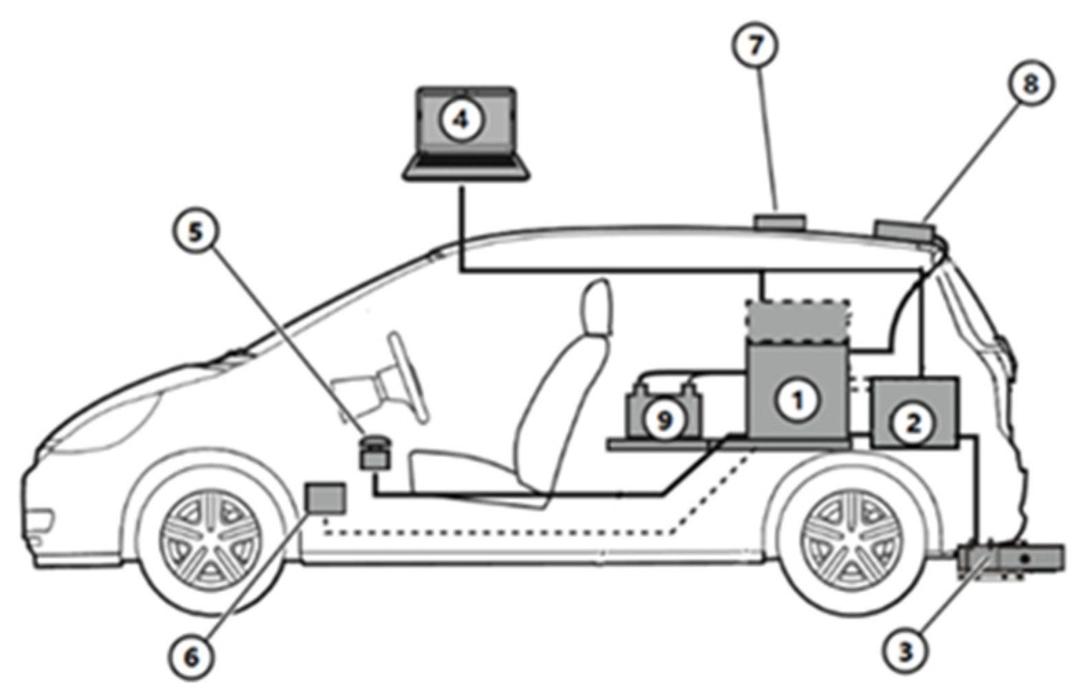
OBS-ONE consists of three main components: a gas analysis module, a particle number (PN) analysis module, and an exhaust flow meter. There are also accessories such as a global positioning system (GPS), weather station (temperature and humidity), and OBD communication equipment. The gas analysis module can measure the concentration of pollutant emissions such as CO, CO
2, and NOx. The particle quantity analysis module measures the quantity concentration of particulate matter. The exhaust flow meter measures the real-time flow rate of the exhaust. The GPS and weather station provide information on the speed and altitude of the test vehicle, air temperature, and humidity. The installation of the PEMS equipment on the vehicle under test is shown in
Figure 1.
The OBS-ONE system requires a DC power supply of 22–28 V. Non-Dispersive Infra-Red (NDIR) is used to determine CO and CO
2 concentrations. Chemiluminescence Detection (CLD) is used to determine NOx concentration. A condensation particle counter (CPC) is used to measure PN.
Table 1 summarizes the measurement principle, analyzer range and specifications of zero gas and range gas, and measurement error.
Table 2 shows the environmental conditions for the use of the OBS-ONE system. Use under the specified environmental conditions is required to ensure stable operation of the measurement equipment and measurement accuracy.
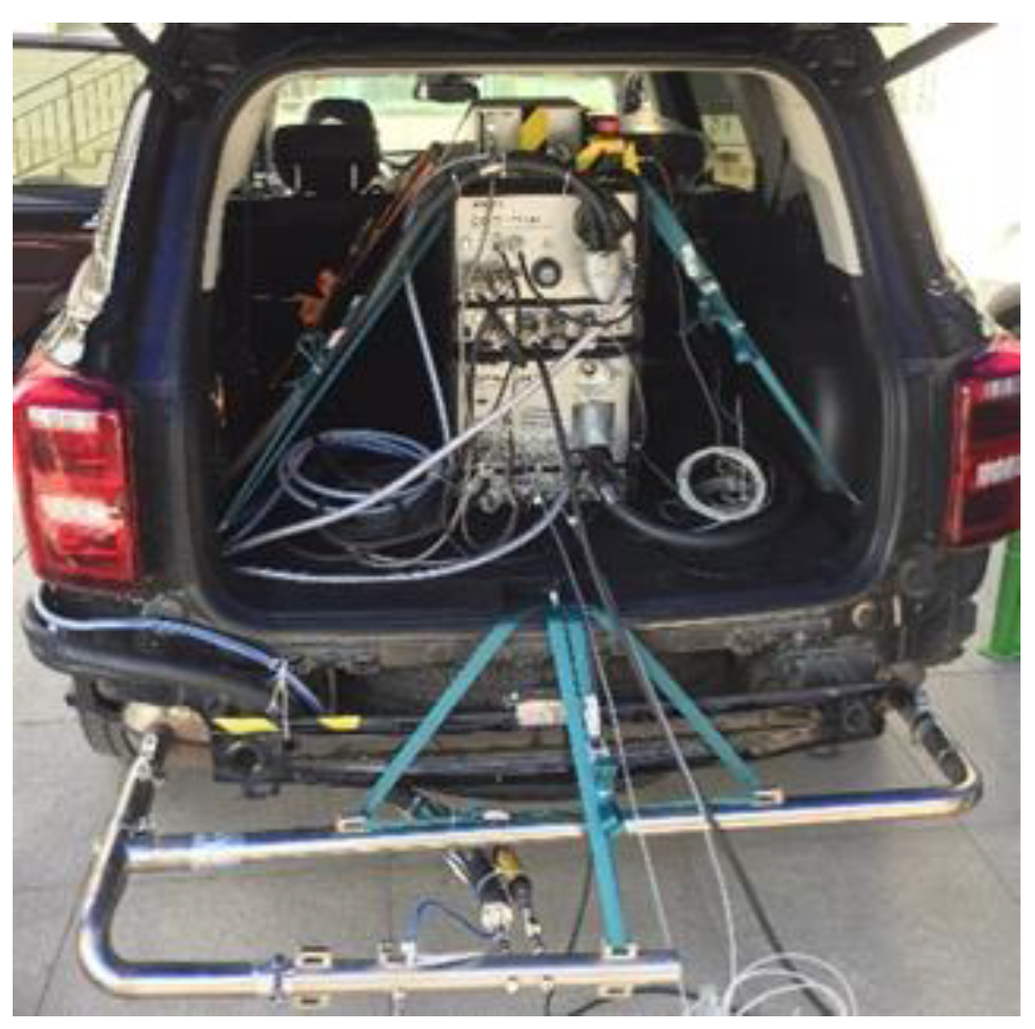
Figure 2 shows the schematic diagram of the OBS-ONE installation of the test vehicle before the start of the test. The specific parameters and atmospheric conditions of the vehicle are shown in
Table 3.
Before the RDE test, the PEMS should be warmed up. Then, the leaks should be checked and calibrated. The zero and span gas are used to calibrate the gas analyzer.
The test equipment records data before the engine starts for the first time, and the whole process records the pollutant concentration, vehicle position, environmental conditions, etc., without interruption.
The vehicle should be driven under the specified test conditions.When the test meets the requirements of
Table 4 is possible to stop the experiment. To ensure data accuracy, the gas analyzer should be checked after stopping recording data.
2.2. Experimental Data Processing
Due to the influence of exhaust flow rate, exhaust temperature, and pressure, length of sampling pipeline, the time sequence of sample gas entering different analyzers, and different response times of analyzers, there are timing inconsistencies between various pollutant concentration parameters recorded in the test and engine speed and vehicle speed values (which can be read by GPS or OBD interface), so it is necessary to perform time alignment of transient data to obtain various parameters generated at the exact moment, and perform pollutant mass emission calculations based on the aligned flow and concentration data. In addition, it is necessary to perform pollutant mass emission calculations based on the aligned flow and concentration data. In this study, the PEMS equipment has an automatic time series correction function, and the raw data of transient mass emission of each pollutant is the result of the correction, which can be directly used for further analysis and processing.
After the time sequence calibration, the invalid data should be eliminated, including the data during the PEMS equipment inspection and zero-point drift verification; the data during the cold engine start, i.e., when the coolant reaches 70 °C after the engine ignition or when the coolant temperature changes less than 2 °C within 5 min.
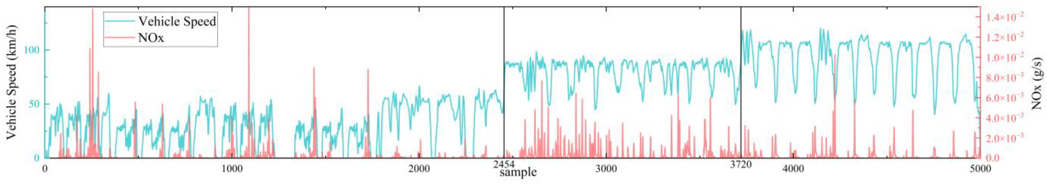
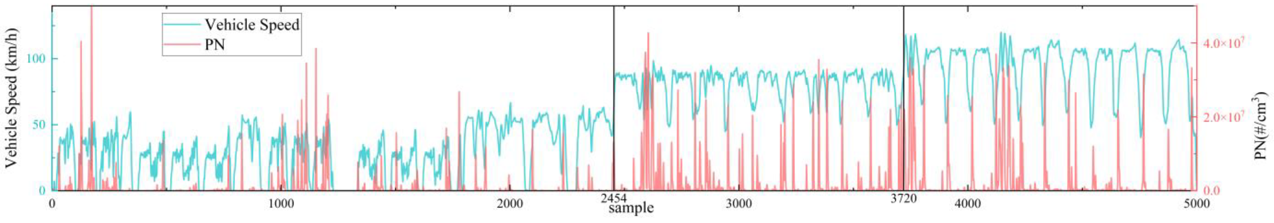
Figure 3 and
Figure 4 show the NOx and PN at the vehicle speed and the corresponding vehicle speed, respectively. It can be seen that the data correspond to the worse PN and NOx emissions of the test vehicle. Among them, 2454 and 3720 correspond to the switching between urban, suburban, and high-speed conditions. It can be seen that the NOx and PN emissions are significantly different under different working conditions.
3. Neural Network Prediction Model Building
3.1. Selection of Model Parameters
The prediction model uses a total of 5000 sets with an interval of 1 s between each data set. To prevent overfitting and to improve the generalization ability [
35], all sample data are randomly divided into three parts: 80% of the training set, 10% of the validation set, and 10% of the prediction set.
RDE experiments have more influencing factors, and too many inputs lead to long prediction times and low prediction accuracy [
36].
The engine speed affects the vehicle speed and acceleration; the vehicle speed, acceleration, and specific power have pronounced effects on emissions; the fuel consumption value, exhaust temperature, and exhaust flow can reflect the combustion situation, all of which will have an impact on emissions. Therefore, the above inputs must be considered when building NOx and PN prediction models.
In this study, principal component analysis is used to extract features from the input parameters to eliminate the correlation of the original data and reduce the dimensionality of the data [
37].
3.2. Structure of Neural Network
As an important branch of intelligent algorithms, NN are widely used in the fields of information processing, pattern recognition, and system control. NN models can better solve complex problems such as non-linearity and multiaxiality in actual road emissions.
BP NN is a multilayer feed-forward NN with a wide range of applications in the engineering field [
38].
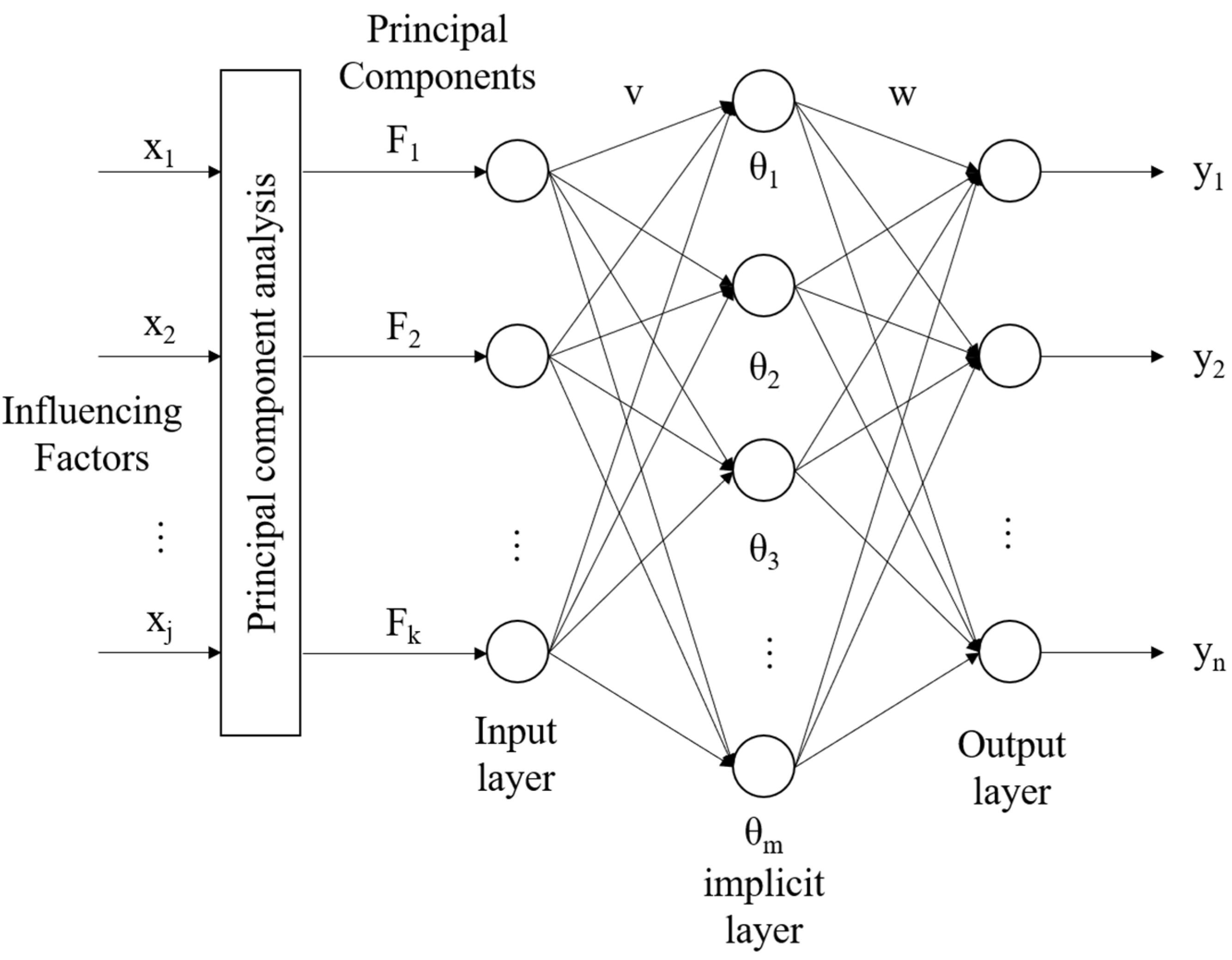
The NN structure used in this paper consists of an input layer, a hidden layer, and an output layer, as shown in
Figure 5.
The input layer is , which uses exhaust flow, exhaust temperature, engine speed, and vehicle speed, which have a significant impact on emissions. is the principal component score obtained after processing. is the hidden layer, the number of hidden layers can be adjusted according to the research problem. is the output layer that characterizes emissions such as NOx, and PN. V and W are the weight of each layer, respectively.
The tansig function is used from the input layer to the hidden layer, and the purelin function is used from the hidden layer to the output layer. The number of nodes in the hidden layer needs to be selected according to the error.
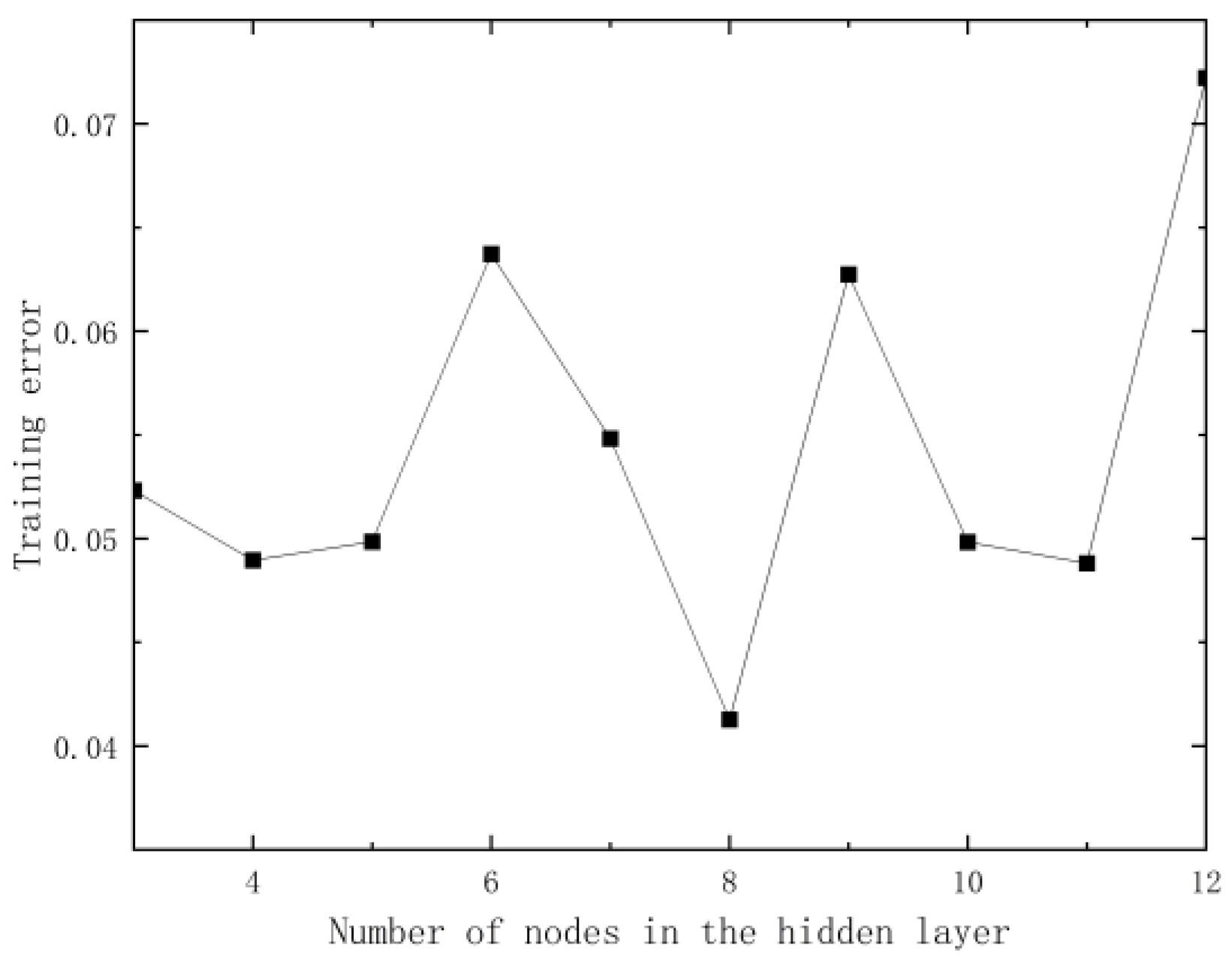
Usually, increasing the number of hidden layer nodes can improve prediction accuracy. However, too many nodes in the hidden layer increase the complexity of the model and even lead to overfitting.
To balance the prediction accuracy and the complexity of the model, the model uses random initial weights by comparing the effects of different numbers of nodes on the prediction ability of the model, as shown in
Figure 6. The number of nodes in the hidden layer corresponding to the minimum training error is finally chosen to build the prediction model.
3.3. BP Neural Networks Optimizing with GA
GA is a heuristic algorithm widely used in various engineering optimization problems [
39].
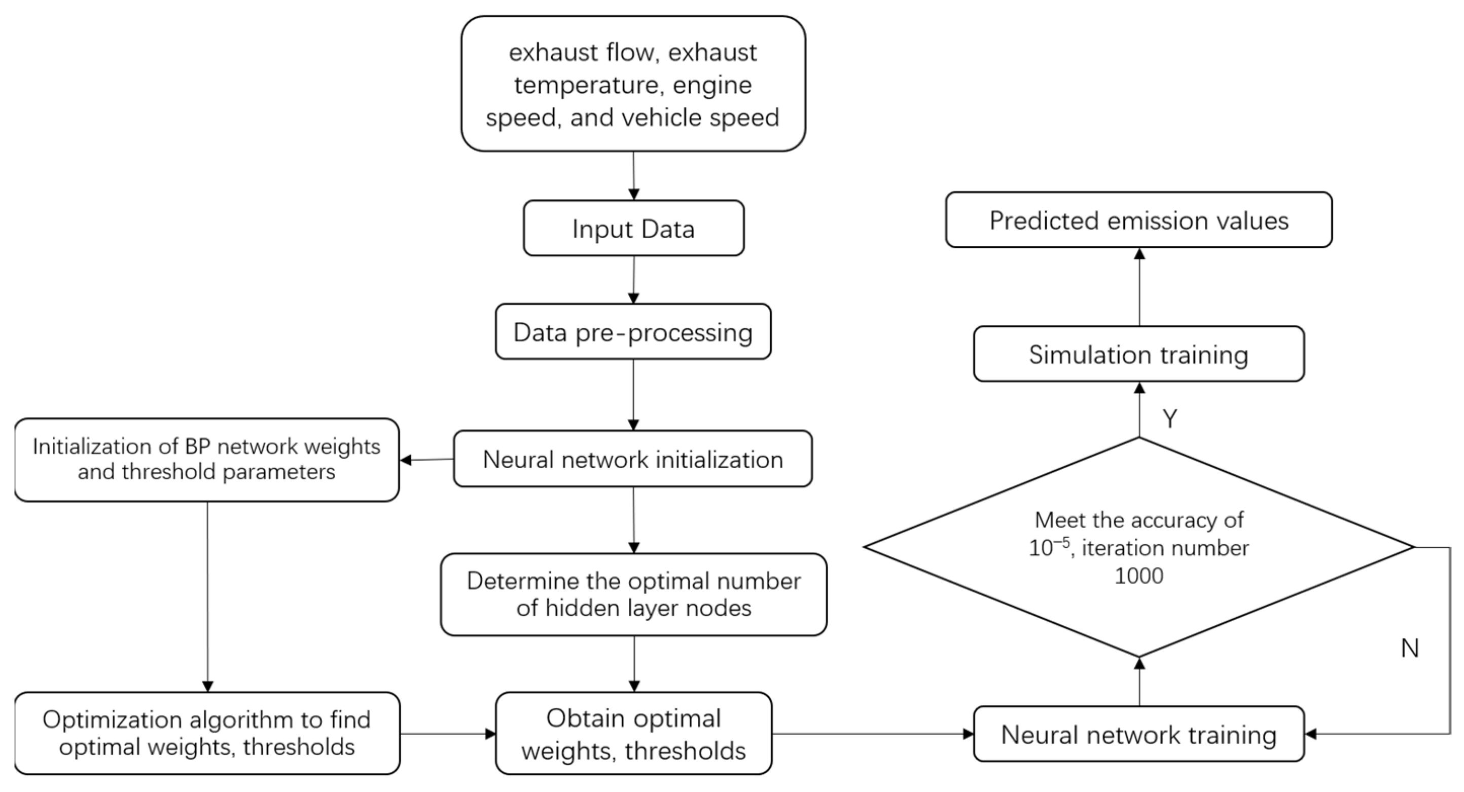
GA-BP means that the weights of the BP NN are optimized using GA, and the optimal result is used to train the BP model. The flowcharts of the GA-BP NN model are shown in
Figure 7.
The specific steps are as follows [
40].
- (1)
Encoding: Encoding converts the solution of the problem to be optimized into a spatial search that can be solved by the GA.
- (2)
Initialize the population.
- (3)
Adaptation function: The fitness function is set as the absolute value of the error between the output predicted value and the output expected value, and the calculation formula is:
where,
F is the fitness value,
h is the dimensionless coefficient,
n is the number of nodes, and
yi, oi is the output expectation and output prediction of the
i node, respectively.
- (4)
Selection: The selection operation is to simulate the process of completing the natural elimination of individuals of biological populations in the process of genetic evolution. In this paper, the roulette wheel method is used as the selection operator, and the optimal individuals are retained after screening, then the selection probability for each individual is calculated by the formula
where,
Pi is the selection probability,
fi is the inverse of the individual fitness value,
u is the dimensionless coefficient, and
Q is the total number of individuals in the population.
The optimized weights and thresholds are obtained by the GA after completing the above steps and brought into the BP NN to start the prediction.
3.4. Analysis of Model Prediction Results
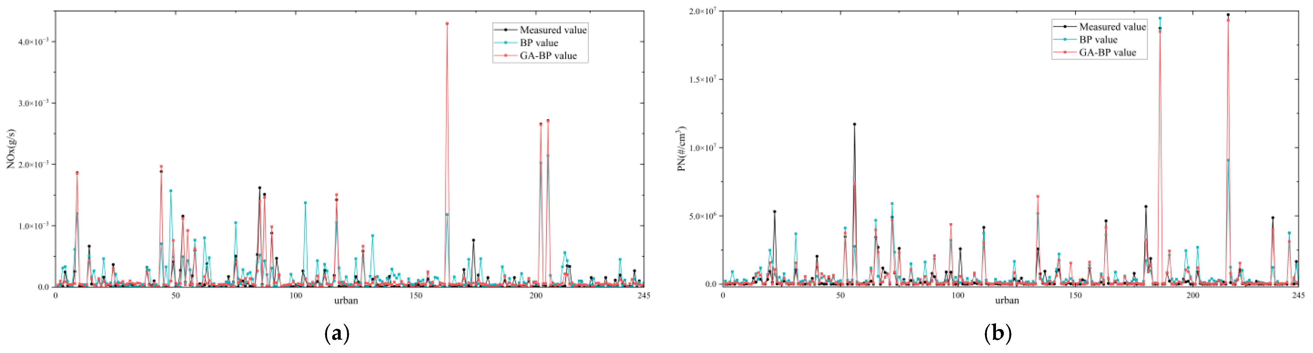
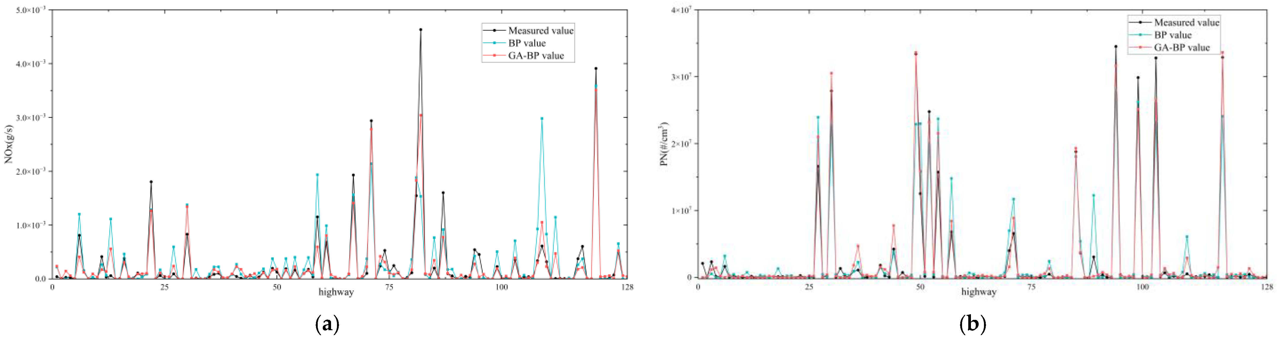
The prediction set is divided according to the percentage of different working conditions in the whole test. There are 500 sets of data in the prediction set, including 245 sets for urban areas, 127 sets for suburban areas, and 128 sets for highways. The BP and GA-BP NN prediction results for the three operating conditions are compared with the measured values, as shown in
Figure 8,
Figure 9 and
Figure 10.
Figure 8,
Figure 9 and
Figure 10 show that the BP NN model fails to correspond well at the more prominent peaks and has significant errors with the measured values. Its prediction at smaller values is substantially and significantly higher than the measured values.
Observing the prediction results of the GA-BP NN model for pollutants shows a significant improvement in its fit with the measured values at the peak. Although there are still large individual deviations, the number is sparse. At the same time, small values can be predicted to fit the measured values better.
To further assess the accuracy of the model for transient prediction. The analysis is performed using the coefficient of determination
R2, expressing the correlation between the two data variables. The coefficient of determination
R2 is calculated as follows:
where,
Xi is the measured value;
Yi is the predicted value.
The correlation between the two sets of variables in the formula is generally considered significant when the coefficient of determination R2 is higher than 0.7. The closer the R2 is to 1, the stronger the correlation is.
Table 5 shows the coefficients of determination
R2 between the results of the two models for NOx and PN predictions and the measured values under different operating conditions. The BP model has high accuracy for the transient prediction of PN, but the transient prediction of NOx is very unsatisfactory, with the lowest
R2 of 0.4832.
Compared with the prediction results of the BP model, the GA-BP model has significantly improved the coefficients of determination for NOx and PN predictions. The lowest R2 of GA-BP for NOx prediction is 0.9062. It can be considered that the established GA-BP model has high accuracy in predicting the instantaneous emissions of light-duty vehicles.
Table 6 and
Table 7 compare the predicted results of the BP and GA-BP models for NOx and PN with the measured values, respectively. The prediction accuracy of NOx is improved from the maximum error of 15.83% in the BP model to 6.84% in the GA-BP model. The prediction accuracy of PN is improved from the maximum error of 9.88% for the BP model to 5.38% for the GA-BP model.
The main reason for the error may be that the model is poorly fitted overall for the small value part in response to the sudden peak. Environmental factors ignored by the model and post-processing devices may also make the error larger.
However, observing the results, it can be found that the error sizes are within acceptable limits, and the established GA-BP model can be considered to have a high accuracy in predicting the overall emissions of light-duty vehicles.


