Article

A Bivariate Nonstationary Extreme Values Analysis of Skew Surge and Significant Wave Height in the English Channel

Institute for Radiological Protection and Nuclear Safety, 92032 Fontenay-aux-Roses, France
*
Author to whom correspondence should be addressed.
Atmosphere 2022, 13(11), 1795; https://doi.org/10.3390/atmos13111795
Submission received: 23 August 2022 / Revised: 19 October 2022 / Accepted: 27 October 2022 / Published: 30 October 2022
(This article belongs to the Special Issue Multi-Hazard Risk Assessment)

Abstract

:
Coastal flooding compound events can be caused by climate-driven extremes of storm surges and waves. To assess the risk associated with these events in the context of climate variability, the bivariate extremes of skew surge (S) and significant wave height (HS) are modeled in a nonstationary framework using physical atmospheric/oceanic parameters as covariates (atmospheric pressure, wind speed and sea surface temperature). This bivariate nonstationary distribution is modeled using a threshold-based approach for the margins of S and HS and a dynamic copula for their dependence structure. Among the covariates considered, atmospheric pressure and related wind speed are primary forcings for the margins of S and HS, but temperature is the main positive forcing of their dependence. This latter relation implies an increasing risk of compound events of S and HS for the studied site in the context of increasing global temperature.

1. Introduction

Of the many human activities located on littorals, which are all at risk of coastal flooding, nuclear power plants (NPPs) are among the most important given the potential for disaster. The French Institute for Radiological Protection and Nuclear Safety (IRSN) is charged with assessing the risk to the country’s coastal NPPs. As a concrete example, the Blayais NPP, located in the estuary of the Gironde, one of France’s main rivers, was subject to a coastal flooding during the winter of 1999, caused by simultaneous high tide, high waves and storm surge [1]. The flood protection of french NPPs has since been upgraded, but given the multivariate nature of coastal flooding and the context of climate change, risk assessment remains an ongoing research subject, which is the purpose of the present study.
As in the Blayais example, coastal flooding events are more often produced by a combination of several factors rather than a single one, and are thus compound events in most cases [2]. Climate-driven extremes are among the main causes of coastal flooding through storm surges and wind-waves [3]. Other major factors are high tides and sea level rise. When these factors are positively correlated, analyzing them separately in a univariate framework underestimates the associated risk [4]. Less- or un-correlated factors can also simultaneously reach a high level and thus should be considered jointly. In the case of coastal flooding, the potential causes are numerous, with some factors depending on the site (e.g., fluvial flooding, rainfall, and rising water table). Vousdoukas et al. [3] analyzed the main causes of coastal flooding common to any site for a global projection of extreme sea levels, with sea level rise, tidal components and water level variations caused by climate extremes—the latter regrouping storm surge and wave height. Rueda et al. [2] studied climate-driven oceanic components with a joint analysis of storm surge, wave height and wave period using a methodology based on spatial patterns of atmospheric pressure. The present study considers only the storm surge (denoted ’S’ and referring to the skew surge thereafter) and the significant wave height (HS). Since these two variables can combine into compound events, their dependence must be taken into account. A copula was used to model this dependence structure between S and HS.
Extreme values analysis is done with either a block maxima (block of time, e.g., the yearly maxima) or a threshold approach. The former is widely used, with the generalized extreme value (GEV) distribution of typically yearly maxima. The latter threshold approach—using either the generalized Pareto (GP) distribution or the nonhomogeneous Poisson process (NHPP)—is less employed, in part because of the difficulty of selecting an appropriate threshold, but it allows better usage of data [5]. The block size choice in the block maxima approach is analogous to the choice of the threshold [6], so the need to select an appropriate threshold—with its associated uncertainty—should not be perceived as a more arbitrary approach (even if the block size is constrained by the sample frequency, the choice is then made in the sampling scheme). The NHPP model has the same parameterization as the GEV distribution, with parameters of location, scale and shape, whereas the GP distribution only has a scale parameter dependent on the threshold value and a shape parameter. This gives an advantage to the NHPP model for nonstationary modeling, which is detailed in the next paragraph. Therefore, we use the threshold approach with the NHPP model for the extremes of S and HS [7].
Since S and HS are the climate-driven components of coastal flooding, their analysis needs to account for the nonstationarity induced by both climate oscillations at different time-scales and the long-term trend of climate change. Nonstationary modeling of extreme values is usually achieved by having the distribution’s parameters depend on covariates [8]. These covariates can be purely mathematical objects, such as a cosine wave to model a cyclic variation or a low-order polynomial for a trend, but can themselves also be physical signals. Such physical covariates can correspond to large-scale atmospheric/oceanic phenomenon, for example an El Niño–Southern Oscillation index [8] or a large-scale circulation index specially defined for the analysis of a given variable [9]. Instead of mathematical objects or large-scale circulation indexes, we extract time series from gridded reanalysis data of atmospheric parameters to use as covariates. We assume that if these atmospheric parameters are drivers of S and HS, the eventual oscillations and long-term trends of these parameters should also be present in the variables. When considering a nonstationary model, establishing a link between such covariates and the variables let the former “carry” the eventual oscillations and trends, making it unnecessary to explicitly introduce these oscillations and trends in the model (e.g., if the wind is a forcing of the waves and both have a marked seasonal cycle, introducing the wind as covariate to model the waves also introduces seasonality in the model, making it unnecessary to introduce seasonality as a cosine wave). This approach is prone to spurious associations that can be caused by a frequency common to variables and covariates without a physical link between the two, most notably with the seasonal cycle that is present in many geophysical signals. Therefore, thorough exploratory analysis is required prior to modeling—which is also true for any approach. The additional uncertainties that accompany the definition of trends by mathematical objects (be it low-order polynomials or regime shifts) make this approach subject to criticism [10]. We chose to let these trends be carried by atmospheric parameters (or indexes) to leverage the rich work on climate reanalysis and projections. Once a robust relation between a given variable and an atmospheric covariate has been established, the projections of this covariate—which includes its eventual trend—can be used for future inferences. Of course, this approach is also accompanied by numerous sources of uncertainties, but it can give more physical meaning to the nonstationary analysis and thus the inferences. The possible impact of atmospheric covariates on the extreme values of S and HS is taken into account by letting the three NHPP model parameters depend on these covariates. Similarly, these covariates could influence the dependence between the variables, which can be accounted for by a dynamic copula (i.e., a nonstationary copula). As in the nonstationary version of the NHPP model, the parameters of the copula can depend on covariates.
The shape parameter of the extreme value distribution is the most important one, as it governs the behavior of its tail, from which extrapolation is made. Most studies using nonstationary models consider time-varying location and/or scale parameters but keep the shape parameter constant, sometimes justifying this by the difficulty of accurately estimating this parameter, even when kept constant [11,12]. As an example, the manual of the R package extRemes advises against using a covariate-dependent shape, but it mentions that it could make sense in some situations [13]. Northrop et al. [7] demonstrated their method while keeping a constant shape for simplicity, but they mentioned in their introduction that a time-varying shape could be desirable, e.g., to account for seasonality. They referred to the work of Coles and Pericchi [14], who modeled extreme rainfall using a shape with different values for two seasons, resulting in a parameter taking a higher positive value for the season associated with the most extreme events and thus a heavier upper tail of the distribution for this season. More recently, Ouarda and Charron [15] also advocated for a time-varying shape, demonstrating it with models improved by having this parameter depend on large-scale climatic indexes. Therefore, we allowed the shape parameter to be dependent on physical covariates in our modeling of the extreme S and HS, similar to the location and scale parameters.
In summary, our methodology was (1) to extract time series from gridded atmospheric/oceanic reanalysis data to serve as covariates; (2) to assess whether these covariates could be forcings of the variables or would lead to spurious association by decomposing the signals in various frequencies and comparing them; (3) to model a bivariate nonstationary distribution of S and HS extreme values with the previously selected atmospheric/oceanic parameters as covariates, using the NHPP model for the margins and a dynamic copula for the dependence structure; and (4) to assess the coherence of the model by computing the value of a high quantile given different meteorological conditions.
Our ultimate goal would be to build a multivariate model with all the relevant factors of coastal flooding for a given site (here this site is Dieppe, but the methods should be applicable elsewhere), accounting for nonstationarity and uncertainties, and using it for future inferences. Realistically, the scope of this study is much more limited, and we focused only on the climate-driven oceanic factors S and HS, taking into account the nonstationary and compound aspects of these two variables. Despite this limited scope, this subobjective is itself far from met, and our present results have numerous limitations. We did not consider the uncertainties of our model or use it for future inferences because the aforementioned limitations need to be addressed before reaching these steps. Nonetheless, some progress has been achieved.
Section 2 presents the data and methods used for the nonstationary analysis of extreme values of S and HS. The resulting model is presented in Section 3. Section 4 discusses these results in light of other studies and how this work could be further developed. Section 5 concludes the paper.

2. Materials and Methods
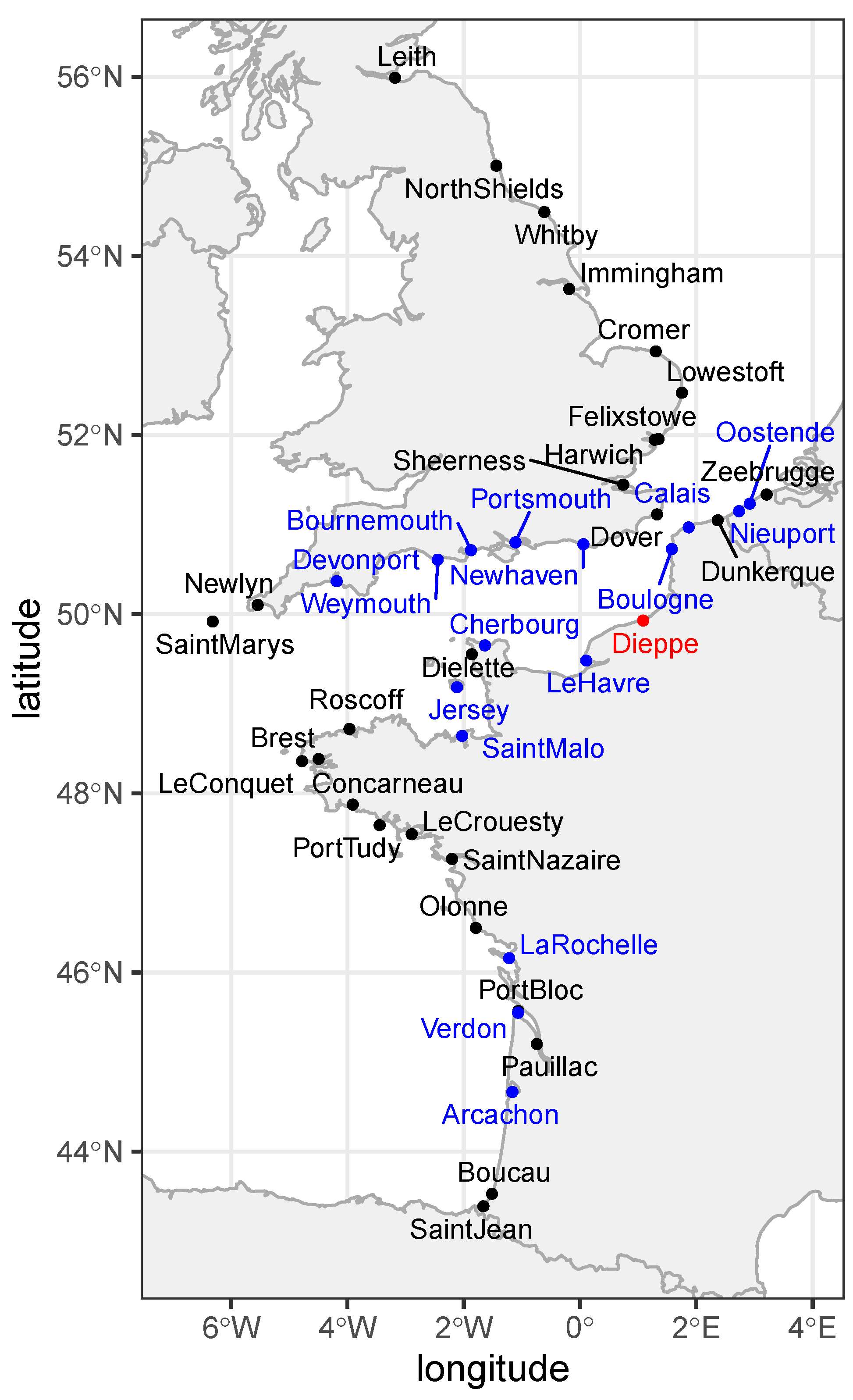
2.1. Data

The S time series was extracted from the sea level measured by a tide gauge located in Dieppe, at 49.92917° N 1.08449° E. The skew surge is defined as the difference between the maximal observed sea level and the predicted astronomical high tide, resulting in an approximately 12 h and 25 min time step. Since this S time series had significant gaps in measurements, regional information from neighboring tide gauges was used for imputation. The extremogram approach was used to define a region of neighboring tide gauges centered on the target site Dieppe with a proportion of common extreme events above a given threshold. For this purpose, extreme events were defined as observations above the quantile 0.99 [16], and the proportion threshold of common events was chosen as 0.3 [17], meaning neighbor stations included in the region had at least 30% of extreme events common with Dieppe (Figure 1). Once this region had been defined, its neighbor stations’ S time series were used to impute Dieppe’s one with a multiple linear regression. The spatial extremogram method for regionalization applied to S is presented in detail in Hamdi et al. [16] and Andreevsky et al. [17]. The daily maximum S was then computed and used for the extreme values analysis.
The HS time series analyzed was extracted from the ERA5 reanalysis hourly dataset [18] using the significant height of combined wind waves and swell. The spatial resolution of this dataset is 0.5° × 0.5° for ocean waves. The HS time series was taken from the grid point 50°N 1°E, which is closest to Dieppe’s tide gauge. Similarly to the S, the daily maximum HS was subsequently analyzed.
Both variables have a strong seasonal component, with their highest values in winter (Figure 2).
The ERA5 reanalysis hourly dataset was also used to have fields of sea level pressure (SLP), near-surface wind speed (NWS, computed from the u and v components of the wind at 10 m) and sea surface temperature (SST). This dataset has a 0.25° × 0.25° spatial resolution for atmospheric variables. These three fields were used to extract covariate time series from specific coordinates. The daily mean values of the time series for a given coordinate were then used for the nonstationary extreme values analysis.
The common period from 1 January 1971 to 17 January 2017 (46 years) was used for all these time series. This choice was constrained by the S time series, for which reliable regionalization results were obtained only between these dates.

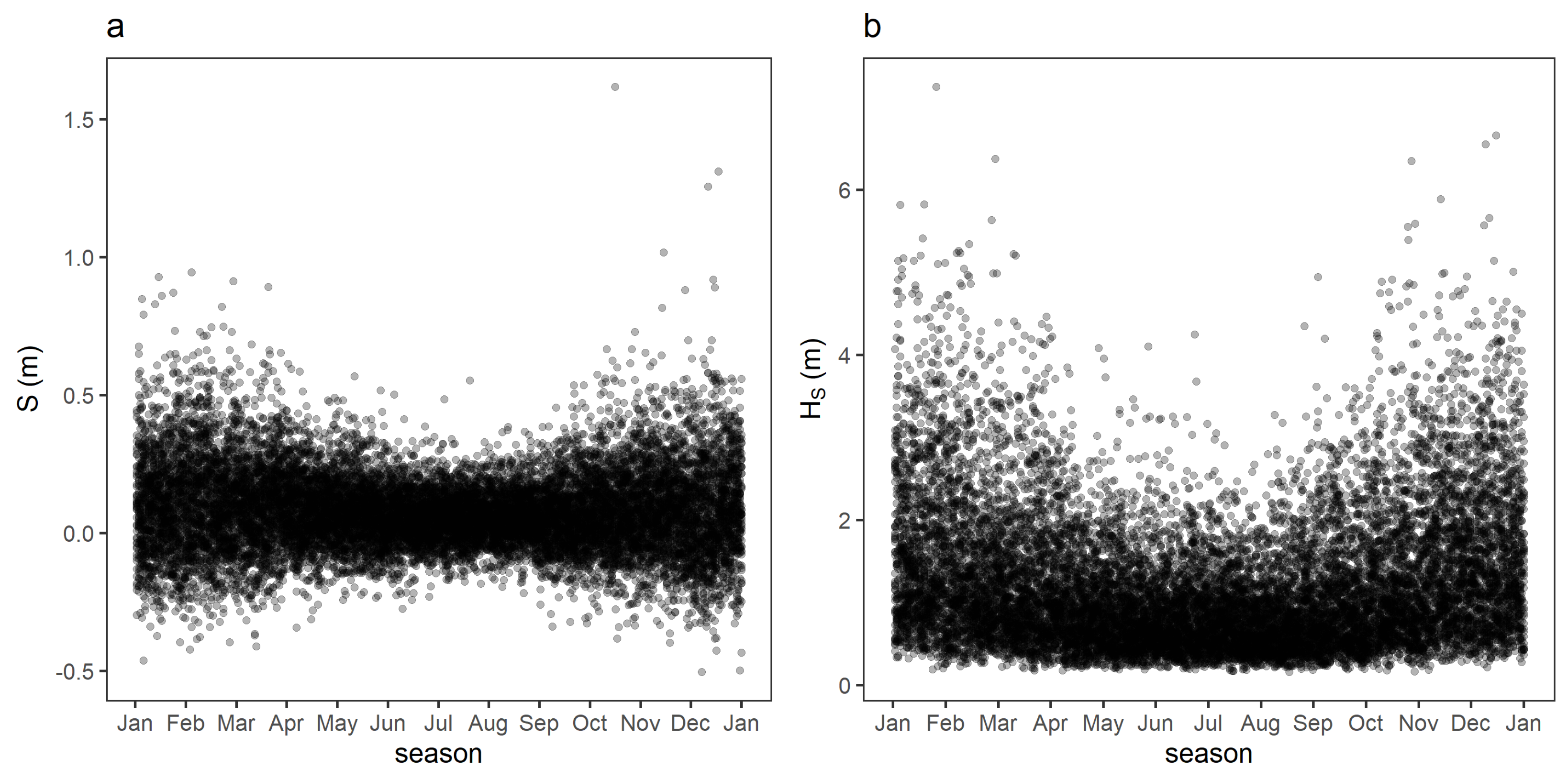
2.2. Exploratory Analysis

It was necessary to select coordinates in the field data sets from which to extract the covariate time series. Different coordinates were selected for each combination of variables (S and HS) and covariates (SLP, NWS and SST). Since the joint distribution of these variables was analyzed in addition to their margins, their product S × HS (HS being strictly positive and both variables having their associated risk for their upper values) was also used as their interaction for covariate selection. This selection was done by computing the pointwise correlation coefficient (Pearson’s ρ ) then extracting the covariate time series from the coordinate of maximal absolute correlation. Since the seasonal cycle is strong in most of these variables and covariates, it was subtracted from them by modeling it with a cosine wave given by s e a s o n = α cos ( d ) + β sin ( d ) , where d is the day of the year scaled to ( 0 , 2 π ) . The pointwise correlation was computed on these residuals, denoted ’A-d’ for variable or covariate A. These coordinates were searched in the subdomain 40°–70° N 25° W–12° E. We assumed that there were no coordinates with higher absolute correlations than those selected outside this subdomain.
The relationship between the selected covariate time series and their corresponding variables was then analyzed for different timescales by complete ensemble empirical mode decomposition with adaptive noise (CEEMDAN) [19] using the R package Rlibeemd (v. 1.4.2) [20]. This signal decomposition method is used to avoid spurious association with covariates that would only have a seasonal frequency in common with the variables (Figure 2), which would imply no relevant relationship. CEEMDAN is a modified version of ensemble empirical mode decomposition (EEMD), a widely used method developed by Wu and Huang [21]. The signal is decomposed iteratively into several intrinsic mode functions (IMFs) describing its different time-scales of variation of and a final residual that is considered to be the overall trend [22]. EEMD is itself a modified version of empirical mode decomposition that corrects the mode-mixing phenomenon when a given physical frequency is separated into several IMFs, but it introduced new issues, such as an unreliable number of IMFs produced and inexact reconstruction of the original signal, both caused by the random part of the algorithm [23]. The modifications of the CEEMDAN algorithm correct the issues of the EEMD while also producing a lower number of IMFs and a clearer separation of the frequency contained within the signal between signals, allowing better interpretability of their physical meaning. We compared the IMFs of the decomposed signal for each combination of variable and covariate to access their co-oscillations at different time scales. For the SLP, NWS and SST time series extracted from the field datasets to be good candidates as covariates for S, HS or S × HS, it would require them to have noticeable co-oscillations at different time scales, including those of higher or lower frequency than the seasonal cycle.

2.3. Modeling of S and HS Extremes

The margins of S and HS extremes were modeled by NHPP, which simultaneously models the distribution of occurrences and excess values over a high threshold with a two-dimensional point-process [24]. This model has three parameters—location μ b , scale σ b and shape ξ —that correspond to the GEV distribution of the b-year largest value [6]. In a nonstationary analysis, these parameters are dependent on a matrix of covariates X that modify the response of the variable Y. Following the notation in Northrop et al. [7], t refers to the time in days, x t is the value of the covariate vector for day t, and μ b ( x t ) , σ b ( x t ) and ξ ( x t ) are the covariates-dependent parameters, whose notation will be simplified as μ t , σ t and ξ t , respectively.
NHPP models the occurrences and excess values on { ( t , y t ) | t [ 0 , T ] , y t [ u t , ) } , with u t being a high threshold. Its intensity function is
λ b ( t , y t ) = b 1 σ t 1 1 + ξ t y t μ t σ t + 1 / ξ t 1 ,
where for the part between the parentheses, z + = max { z , 0 } . We used b = 1 by default.
The parametric regression used for the NHPP parameters were
μ t = μ 0 + i = 1 n μ μ i U i ,
ϕ t = ϕ 0 + i = 1 n ϕ ϕ i V i ,
ξ t = ξ 0 + i = 1 n ξ ξ i W i ,
where U, V and W are the matrices of normalized covariates for μ t , σ t and ξ t , respectively. The log link function log ( σ t ) = ϕ t keeps the scale parameter positive. The vectors { μ 0 , , μ i } , { ϕ 0 , , ϕ i } and { ξ 0 , , ξ i } , of length n μ , n ϕ and n ξ , respectively, are the regression parameters of the three NHPP model parameters, and are thus referred to as hyperparameters (i.e., parameters of parameters).
The threshold u t can also be covariate-dependent to be set at an appropriate level given different values of the covariates and to have the exceedances spread over a large range of the covariates’ observations, allowing more precise estimation of the covariate’s effect than with a static threshold. As in Northrop et al. [7], this covariate-dependent threshold was set by quantile regression, which estimates the p conditional quantile of a variable Y as a function u ( x , p ) of covariates X. This function is estimated by minimizing
u = p t | r t 0 | r t | + ( 1 p ) t | r t < 0 | r t | ,
with the residuals r t = y t u ( x t , p ) . Northrop et al. [7] used a constrained version of quantile regression to avoid the possibility of crossing the thresholds set for different values of p. This more consistent version of quantile regression was not used in our study. Since the selection of the physical covariates for the NHPP parameters was based on likelihood, it was more convenient to fix the time-varying threshold before the addition of these physical covariates to the nonstationary model. Therefore we defined the covariates used for the quantile regression threshold from the variables themselves, with d the day of the year mapped to ( 0 , 2 π ) and the trend extracted by CEEMDAN, accounting, respectively, for the strong seasonal dependence and the long-term variability of each variable. These thresholds gave an approximate probability p of exceedance throughout the period, independent of the season and the trend, and required no redefinition for different selections of physical covariates.
The estimation of the hyperparameters of the nonstationary NHPP models was done by generalized maximum likelihood (GML), which improves the stability of the estimation by incorporating a Bayesian prior for the shape parameter [25]. The GML was extended to the nonstationary case by El Adlouni et al. [26], who showed its improved performance over the maximum likelihood (ML) estimation for a GEV model with varying location and scale parameters. In our case, attempting to estimate the hyperparameters by ML gave unstable results for some nonstationary models, which were corrected with the GML. Martins and Stedinger [25] proposed a B e t a ( p = 9 , q = 6 ) distribution with support [ 0.5 , 0.5 ] and mean 0.1 as prior. This was not appropriate for our data since the shape parameter was expected to be negative for both S and HS [2]. One reason to use the GML is to obtain a more stable result despite a small sample size, but using a threshold approach resulted in our sample size of exceedances to be slightly above a hundred for both variables. Therefore, a uniform prior with support [ 0.5 , 0.5 ] was chosen to avoid the unstable results but without additional constraint on ξ .
A mixed selection algorithm was used to find the best combination of covariates for each NHPP parameter. This simple procedure starts with the stationary model defined as the current model, then tests all the alternative models defined by the addition of a covariate for a parameter. A likelihood ratio (LR) test is done between the current model and each alternative model. The alternative model whose LR test yields the lowest p-value less than or equal to a significance threshold α is accepted as the new current model, and a new selection step follows, comparing newly defined alternative models to this updated current model. These addition steps are alternated with removal steps, where the alternative models are defined as the removal of one covariate for one parameter and the alternative model whose LR test yields the highest p-value greater than α is accepted as the new current model (if any). The final model is reached when two consecutive addition and removal steps result in no update of the current model. The customary threshold α = 0.05 was used.
The Akaike and Bayesian information criteria (AIC and BIC, respectively) are commonly used in model selection. In the case of nested models, these information criteria are similar to LR tests with different α thresholds that depend on the difference in the number of parameters between the models [27]. For the AIC, the corresponding α 0.16 with one degree of freedom (i.e., one hyperparameter difference between the models, as in the mixed selection procedure described previously). For the BIC, the corresponding α also depends on the sample size; with n = 100 , α 0.032 with one degree of freedom. Therefore selecting among the nested models based on the LR test is equivalent to using one of these information criteria, and the customary value α = 0.05 gives an intermediate significance threshold compared to the AIC and the BIC with a sample size in the hundreds.
The peaks-over-threshold (POT) approach was used to deal with the short-term temporal dependence caused by consecutive exceedances of the threshold during an extreme event. This was done with the runs declustering method [13] with a run length of two to consider a storm event duration of 3 days, as this duration was selected by Camus et al. [28] for an analysis of extreme skew surge (but we used the same value for HS). Note that the POT approach is not the only option for a threshold-based extreme values analysis—for example Fawcett and Walshaw [29] showed that all the exceedances could be analyzed instead of the cluster’s maxima if a correction is applied to the standard error of the parameter estimates, and Li et al. [30] developed a self-exciting marked point process that explicitly models the short-term temporal dependence. Nonetheless this declustering approach was used in our study for simplicity.
The R package extRemes (v. 2.1-2) was used to fit the NHPP model [13].

2.4. Modeling of the Dependence between S and HS

The dependence structure between S and HS was modeled with a dynamic copula. Copulas are multivariate distributions whose margins are all uniform with support [ 0 , 1 ] [31]. The simplest case of a bivariate distribution is given by
F X Y ( x , y ) = C ( F X ( x ) , F Y ( y ) ) ,
where C is the copula with parameter θ (here considering a single parameter copula). A dynamic copula has a covariate-dependent θ to model a varying dependence structure between the variables. Similar to the nonstationary NHPP model used for the margins, this dependence on covariates can be modeled by a parametric regression. The value θ is linked to Kendall’s τ with a specific expression per copula class. Thus, dynamic copulas can be obtained by making τ itself dependent on covariates then computing a varying θ from this dynamic τ [32]. Another option is to have θ directly dependent on covariates [33]. Using the former parameterization, the model considered is analogous to the parametric regression used for the nonstationary NHPP parameters, with
τ t = Λ κ 0 + i = 1 n κ κ i Z i ,
where Z is the matrix of normalized covariates, and Λ ( x ) = ( 1 + e x ) 1 keeps τ t [ 0 , 1 ] —here only considering positive correlation between the variables—and { κ 0 , , κ i } is the vector of hyperparameters of length n κ . The copula is fitted on the daily pseudo-observations, which are the observations mapped to ( 0 , 1 ) using their ranks [34].
The S and HS daily observations have a strong autocorrelation, which should be partially accounted for by the dynamic copula [35], assuming it is caused by the physical covariates’ influence to a certain extent.
Two copula classes with a non-null upper-tail dependence (UTD) and a single parameter, the Gumbel and Joe copulas, were tested because S and HS are positively correlated and we studied their upper extremes [33].
Model selection for the dynamic copula was done with a mixed selection algorithm similar to that used for the NHPP models. The best class between the Gumbel and Joe copulas was selected prior to the mixed selection by comparing the results with those of stationary copulas.
A rolling window (also called running window) Kendall’s τ was computed from the observations of S and HS with a one year window span to compare it to the covariate-dependent copula parameter θ (and its corresponding τ ) obtained with the dynamic copula [33]. The high frequencies of both time series were filtered by locally estimated scatterplot smoothing (LOESS) for readability. For the model to be adequate, the empirical varying τ obtained with the rolling window and the dynamic copula parameter should correspond for the low frequencies (i.e., fluctuations of pluriannual time scale).
The R packages VineCopula (v. 2.4.4) [34] and copula (v. 1.1-0) [31] were used to fit the copula and assemble the multivariate distribution.

2.5. Definition of the p-Level Curves

Since the marginal distributions correspond to yearly probabilities, whereas the copula distribution correspond to daily probabilities, one or the other must be converted to assemble a bivariate distribution with a common time referential. We chose to use a yearly probability, as this is the most common choice and is implemented in the R package extRemes (v. 2.1-2) [13], but using daily probabilities could be more sensible since our variables and covariates all have a daily time-step. The yearly probability p was converted to the copula daily referential with p d a y = p 1 / 365.25 .
The definition of the p-level bivariate quantile used is
p : = P [ X x Y y ] = F X Y ( x , y ) ,
which considers a hazard scenario to be defined as both variables simultaneously reaching a high quantile [36] and is sometimes called the “and” scenario. A resulting p-level curve has an infinite number of points with the same probability of simultaneous non-exceedance but different probabilities of occurrence since this curve intersects the bivariate distribution’s density isolines. The highest density point along a p-level curve was estimated numerically using the conditional distribution of Volpi and Fiori [37] for each day of the observation period to assess how climate variations affect the p-level obtained with the nonstationary distribution. Doing this with the full p-level curves instead, or even a subset of the curve aggregating ( 1 α ) × 100 % of its density, would not produce a readable result with 46 years of daily observations.

3. Results

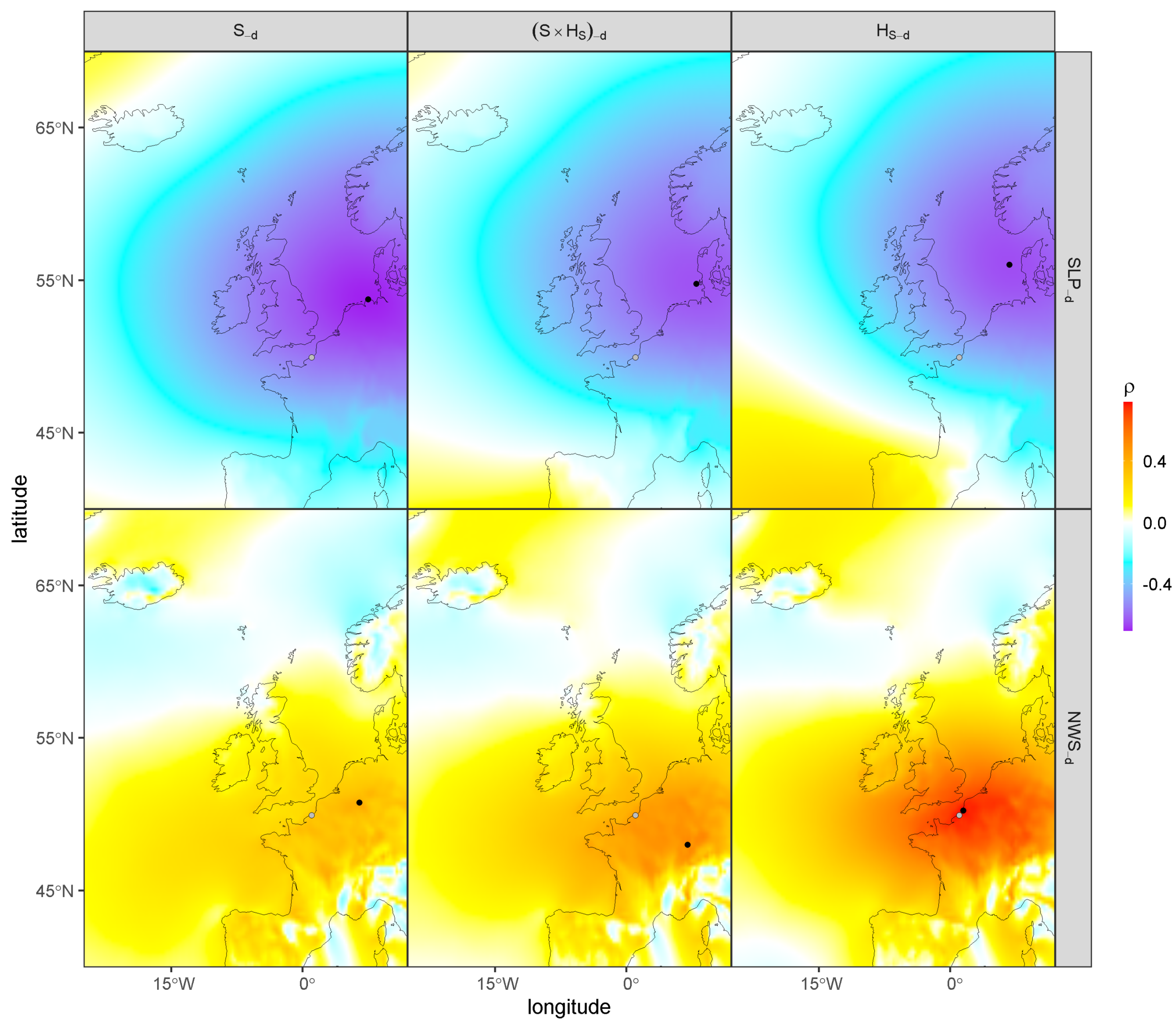
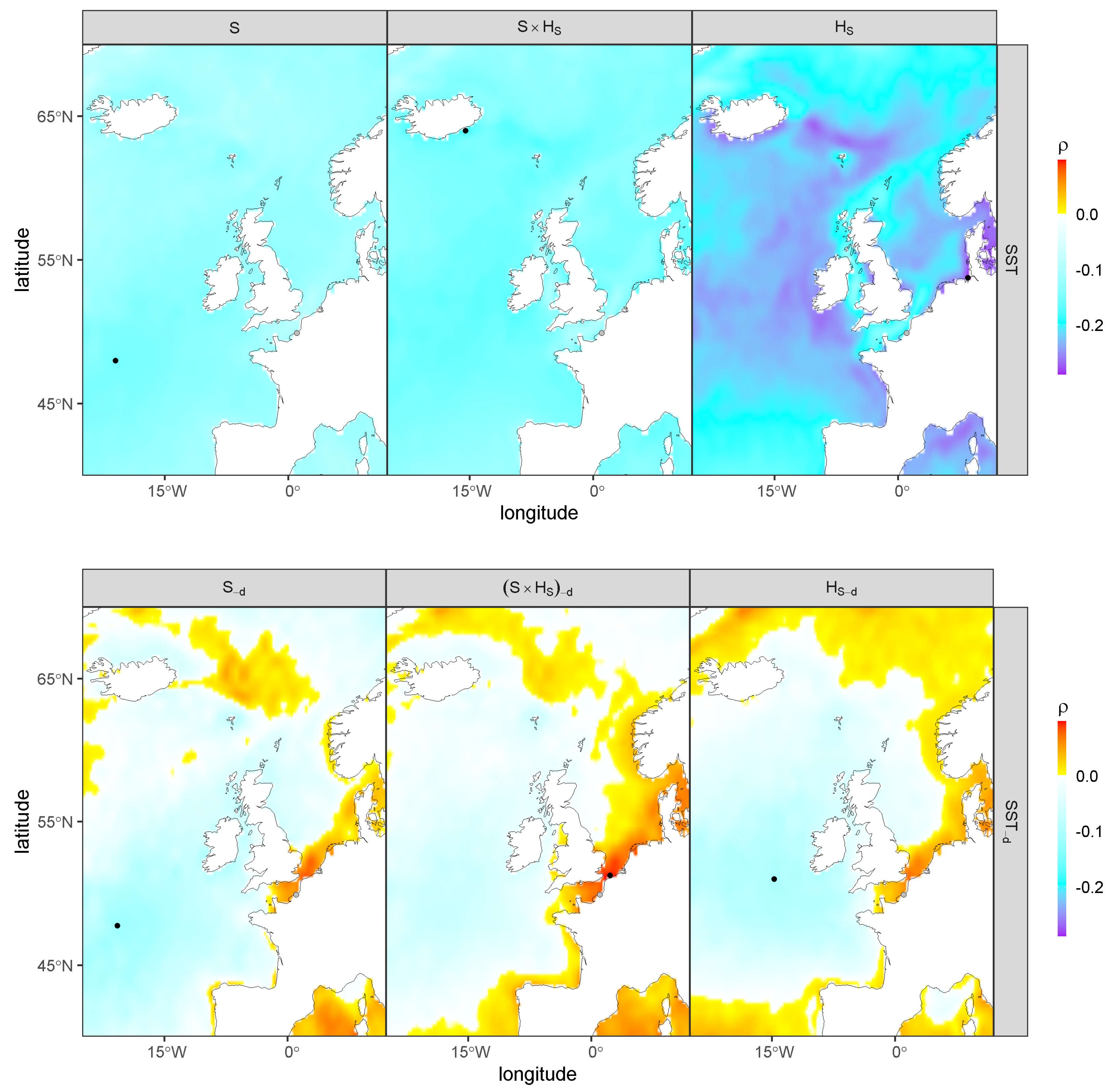
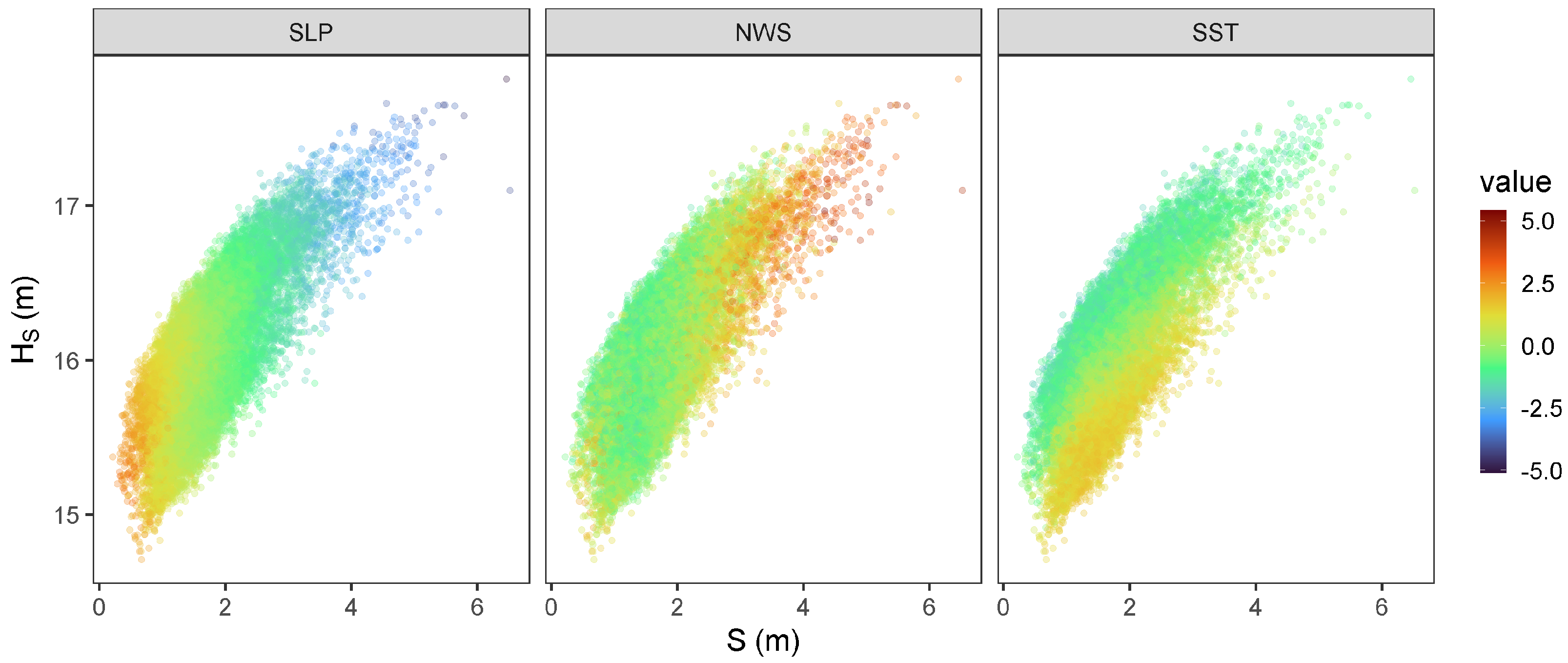
3.1. Pre-Selection of the Physical Covariates

The maps of Figure 3 show the spatial variability of the correlation between the variables S, HS and their interaction S × HS and the two covariate fields SLP and NWS. The black dots indicate the points of maximal absolute correlation from which the covariate time series were extracted. For SLP, this point is located in the southeast part of the North Sea for both variables and for their interaction, with a negative correlation strongest for S. For NWS, this point is located close to the variables’ stations for HS (indicated by the grey dot), but is further in the continent for S and the variables’ interaction, with a positive correlation in each case but highest for HS. The seasonal frequency was removed from both the variables and the covariates, indicated by the d subscript. For these two covariates, the coordinates of highest absolute correlation are not much different if this frequency is not removed.
The maps of Figure 4 are similar for SST, but this time, removing (bottom row) or retaining (top row) the seasonal frequency resulted in a different location of highest absolute correlation. The highest correlation is negative for both variables and their interaction when the raw signals were used. The coordinate picked for S is located in the Atlantic, but those for HS and the variables’ interaction are located on coasts, at locations that appear to have little physical meaning (e.g., on the coast of Iceland for the interaction and Germany for HS). When the variables and the covariates were instead analyzed with their seasonal frequency removed, the coordinates of maximal absolute correlation are similar for S but appear to have more physical meaning for HS and the interaction, with a point also in the Atlantic for the former and one close to the east end of the English Channel for the interaction, this time with a positive correlation. The S-d and HS-d residuals have a positive correlation in this area, but it is stronger in the interaction’s residual. The SST time series used as covariates were extracted from this second set of coordinates (bottom panel of Figure 4).
The decomposed variable, interaction and covariate time series are presented in Figure 5 and Figure 6 (the Figure for HS is not shown but is very similar to the one for S). The grouping of the IMFs in three subplots is for readability only—we chose to present only one year for IMFs 1 to 5 and five years for IMFs 6 to 10, as displaying the full 46 years for these frequencies would render the oscillations unreadable. The group of IMFs 1–5 shows the year with highest value of S or S × HS, as this date gives the clearest example of the eventual co-oscillations at high frequencies between covariates and variables during an extreme event. Similarly, the group of IMFs 6–10 also includes this date. To no surprise, the S and HS signals have co-oscillations of similar amplitudes to those of SLP and NWS for both high and low frequencies (with reference to the annual frequency), since these atmospheric parameters are major forcings of both variables (Figure 5; a similar figure is obtained for HS). These co-oscillations with SLP and NWS are also clearly visible for the interaction of the variables (Figure 6). Similar co-oscillations are not visible for the two variables and the SST covariate, and the amplitude of the IMFs are different, which does not imply any clear link. However, the variable interaction displays clear co-oscillations with SST of similar amplitudes for IMFs 11 and 12 during certain periods—the 1980s and 1990s for both IMFs, then during the 2010s for IMF 11 (Figure 6). On the one hand, these co-oscillations with SST being only visible for the variables’ interaction is potentially due to the fact that the selected covariate coordinates are much closer to the variables’ coordinates, but on the other hand, the area and the amplitude of the positive correlation around the English Channel increases for the interaction compared to each separate variable (Figure 4, bottom). Overall, this indicates that the SST is a valid covariate to test for the dynamic copula. Furthermore, to impact the interaction of the variables, the SST would necessarily have to impact them separately to an extent, so it was also tested as a covariate for the nonstationary NHPP models of the margins.
The residual of the decomposition for S reveals an overall downward trend for the period (Figure 5).

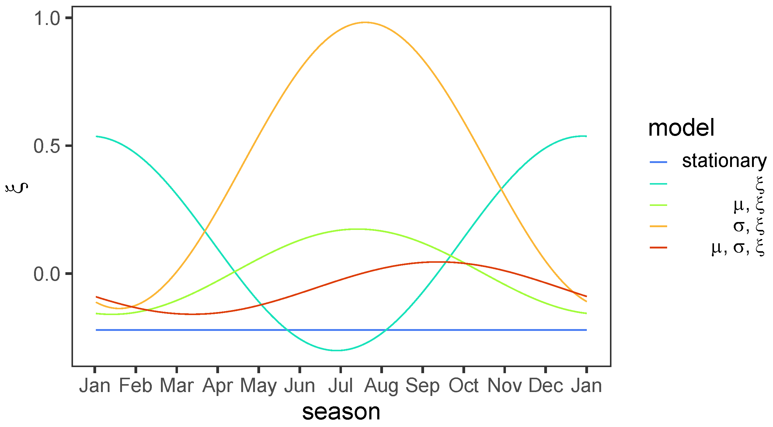
3.2. Nonstationary NHPP for S and HS Extremes

The POT approach resulted in 245 and 261 exceedances of the time-varying thresholds after declustering for S and HS, respectively, for the 46 years of data, corresponding to approximately 5.3 and 5.7 exceedances per year. This higher-than-usual rate of exceedances is obtained for a seasonal-dependent threshold, so a similar number of exceedances during winter (i.e., the season associated with higher values) could be obtained with a constant threshold and lower rate of exceedances.
Table 1 presents the best NHPP model at each step of the mixed selection for S. The final model obtained (Model 5) has a location parameter μ dependent on the three covariates SLP, NWS and SST, a scale parameter σ dependent on SLP and SST, and a constant shape parameter ξ . Table 2 is similar for HS, with a final model with only μ dependent on NWS.
These two mixed selection models were obtained by keeping the shape parameter constant, because otherwise the results were incoherent with the observations. For both S and HS, when covariates were tested for ξ , the final model obtained had a negative effect of NWS on this parameter but a positive impact of this same covariate on μ . For HS, NWS also had a negative effect on σ . These results are cases of overfitting, with a covariate having an effect on a parameter that is compensated for by an effect of an opposite sign on the same—or a similar enough—covariate on another parameter. Since the NWS has a strong seasonal component, these models would result in a higher ξ in summer, which contradicts observations (Figure 2). These issues are not specific to the physical covariates we used and can also be encountered, for example, with seasonal-dependence of the parameters modeled by a cosine wave (see Appendix A).
When ξ is kept constant, the models obtained are consistent with observations and what is expected from these covariates for both variables. The probability of extreme S is greater when SLP is low, along with low SST but high NWS. This NWS covariate is added first for μ during the mixed selection for S, but the absolute value of its hyperparameter decreases at each subsequent step (Table 1). An alternative model corresponding to Model 5 but without μ was tested, but an LR test indicated that the inclusion of this covariate remains significant (p-value of 6 × 10 7 ).
The quantile–quantile plots for each model of the mixed selection for S show that despite it having eight hyperparameters, the fit of the final Model 5 is poor, with most points being overestimated by the model, except the largely underestimated last point (Figure 7). The difficulty of modeling the extreme surge on the French coast of the English Channel is known, which is why Hamdi et al. [16] used both a regionalization approach for missing data imputation and additional historic information to obtain better estimations (with a stationary model). Despite using the same regionalization approach in our study, the final Model 5 obtained with a constant ξ could also be a case of overfitting—the numerous hyperparameters potentially compensating for the difficulties of modeling the extreme surge.
For HS, the final model obtained when ξ is kept constant is Model 1 of Table 2, with only a positive dependency of μ on NWS. The quantile–quantile plots of the mixed selection for HS show that this addition of NWS for μ greatly improves the model compared to the stationary case (Figure 8). This Model 1 for HS has the advantage of being parsimonious, with only one covariate and four hyperparameters, which, by comparison, reinforces the suspicion that Model 5 for S with its eight hyperparameters could be a case of overfitting.
For both variables, the shape parameter is higher for the nonstationary final model compared to the stationary case, and even becomes positive for S (Table 1 and Table 2). This indicates that independent of the meteorological conditions, the highest possible value attained for an extremely rare event could be underestimated in the stationary framework.
The SST covariate has a strong seasonal component, but its clear influence on S has not been established by the exploratory analysis (Figure 5). The residual of the covariate with the seasonal frequency removed (i.e., SST−d) was therefore tested for NHPP models of S to confirm that the variations of SST at frequencies different from the seasonal cycle significantly impact the variable’s extremes. A model analogous to the final Model 5 for S (Table 1) is defined, but with SST−d instead of the full covariate signal, resulting in the parameterization μ t = μ 0 + μ 1 S L P + μ 2 N W S + μ 3 S S T d , ϕ t = ϕ 0 + ϕ 1 S L P + ϕ 2 S S T d , ξ t = ξ . This model is compared to a simpler one without the covariate SST−d for μ and σ . An LR test between these model yields a p-value of 1, indicating that SST−d does not add any significant information to the model, therefore implying that the inclusion of SST in the nonstationary NHPP model for S was a spurious association. The test was conducted anew without SLP, with a model parameterized μ t = μ 0 + μ 1 N W S + μ 2 S S T d , ϕ t = ϕ 0 + ϕ 1 S S T d , ξ t = ξ , which is compared to another model with only NWS for μ . The LR test for these models yields a p-value of 0.003 , this time indicating a significant improvement of the model with the SST−d covariate (with α = 0.05 ). The lack of significance of the first test is therefore attributed to the loss of explanatory power when using the SST−d residual instead of the full signal. These tests give extra support for having SST as a covariate for the margin of S.

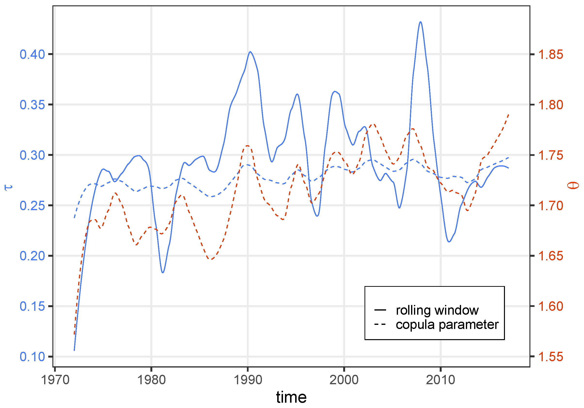
3.3. Dynamic Copula for S and HS

The best stationary copula between the Gumbel and the Joe copulas is the latter, having AICs of 4253.16 and 4536.45 , respectively. The Joe copula was then subsequently used in the mixed selection. Table 3 presents the steps of this mixed selection, with the best model obtained when all three covariates are included.
As for the mixed selection of the NHPP models for S (Table 1), the order in which the covariates are added to the dynamic copula indicates the importance of their impact. Whereas SST was added at later steps for S, as this variable is much more dependent on SLP, the SST covariate is added first for the dynamic copula. Furthermore the SST hyperparameter of the dynamic copula has the highest absolute value, showing its greater influence on the interaction of S and HS compared to the other two covariates (the hyperparameter values being comparable because the covariates are normalized). This is consistent with the exploratory analysis, which showed that the dependence on SST was only visible for the variables’ interaction when using the CEEMDAN decomposition (Figure 5 and Figure 6). The effects of SLP and NWS on the copula parameter θ would partially cancel each other in meteorological conditions associated with a higher p-level (i.e., low SLP but high NWS), leaving SST as the main driver of the dependence structure. Surprisingly, the SLP and NWS effects have the same sign, despite these covariates being negatively correlated. This indicates that having NWS in addition to SLP in the nonstationary model provides relevant extra information.
To avoid any spurious association and to be consistent with the methods used for the margins, a dynamic Joe copula with only the residual SST−d as covariate was compared to a stationary copula. An LR test between those two models yielded a p-value of 3 × 10 13 in favor if the nonstationary one, confirming an increase of the dependence between S and HS as the SST increases.
Figure 9 compares the empirical varying Kendall’s τ between S and HS obtained by rolling window to the varying copula parameter θ and its corresponding τ . The low frequencies (lower than the annual frequency) of the rolling window τ and the copula θ are overall similar for the period, with oscillations corresponding, for the most part, and a common increasing trend. These co-oscillations are the most evident during the 1980s and 1990s, which corresponds to the main period of co-oscillation between SST and the variables’ interaction S × HS seen on the decomposed signal (Figure 6). However, the dynamic copula τ (computed from θ ) has variations of much lower amplitude than the empirical τ , implying that, although the covariates used for the dynamic copula are appropriate, their simple linear effect on θ could not describe the varying dependency well enough.

3.4. Climate-Dependent p-Level of S and HS

The bivariate nonstationary distribution F X Y is obtained by the association of the margins F X and F Y given by the NHPP Models 5 and 1 for S and HS, respectively (Table 1 and Table 2), and the dynamic copula C Model 3 (Table 3), via Equation (6).
The effect of the NWS covariate increases both the levels attained by each variable separately and the probability of simultaneous high levels. On the contrary, the low values of SLP and SST increase the level attained by S but decrease the probability of simultaneous high levels of both variables. Therefore, strong wind conditions appear as the main driver of compound events of S and HS from the perspective of our model. The positive effect of SST on the variables’ dependence implies that this risk of compound events would increase in the context of climate change.
Figure 10 shows the points of highest density along the 0.99 quantile level curves computed for each day of the observations and the corresponding (normalized) covariate values. This illustrates that the climate-dependent p-level obtained is consistent with what is expected from these covariates—the highest bivariate levels were attained for the lowest SLP but highest NWS and low SST. The strong correlation of SLP and NWS results in a similar pattern of variability of these two covariates for the p-levels. This pattern is quite different for SST, with a main direction of variability somewhat orthogonal to that of SLP and NWS, adding support to the idea that SST is complementary to the other covariates.

4. Discussion

Despite its numerous limitations, which will be discussed further below, the bivariate nonstationary model of S and HS is consistent with the results of other studies. Of the three covariates—SLP, NWS and SST—the latter is the most affected by climate change, and therefore introduces its trend in the model. This positive trend is visible both in the SST data we analyzed from 1971 to 2017 (not shown here, but can be seen, for example, in [38] for 1980–2019) and in climate projections (e.g., CMIP6 climate projections), with its future rate of increase depending on the scenario considered. The NHPP model for S has both the location μ and the scale σ parameters dependent on SST and with a negative relation, resulting in a decrease of the level attained for a given probability of exceedance (p-level) over time. Calafat et al. [39] found a similar negative trend during the period 1960–2018 for the extreme surge in the English Channel using a robust spatial approach for trend detection in extremes. This decreasing trend for S in the English Channel could also be explained by the decreasing trend of NWS in the region for the period 1980–2010, but this trend has inverted since that period [38]. Opposite to this decreasing marginal risk associated with S, the positive influence of SST on the dependence of S and HS increases the probability of compound events in the context of climate change. As stated in the introduction, Vousdoukas et al. [3] analyzed he extreme sea-level projections by separating sea-level rise, tidal, and climate-driven extreme components, the latter regrouping both storm surge and waves. They predicted an increase in these climate-driven extremes in the English Channel by 2050 and 2100 under both RCP4.5 and RCP8.5 (Representative Concentration Pathways), with which our results are also consistent thanks to the dynamic copula. The storm surge and wave analysis of Rueda et al. [2] found significant variations of the correlation between S and HS given different spatial patterns of SLP, which is consistent with our dynamic copula having SLP as a covariate, but also with NWS, since these covariates are strongly related.
Many aspects of the present model need major improvements before using it for inferences. The method used for the imputation of the S at a site with the information of neighboring stations relies on multiple linear regression [16], but this could be improved. The threshold of 30% of common events used to define the homogeneous region when using the extremogram method was chosen to be low enough to include observations in the neighboring stations for each time step and because this value was already used for the same data by Andreevsky et al. [17]. The uncertainties related to this threshold were not taken into account, but they require further consideration. In the case of [17], testing different values of the threshold did not significantly change the results of a subsequent extreme values analysis. Once the homogeneous region was defined, one alternative approach instead of multiple linear regression could be to use a vine copula to model the multivariate distribution of S for all the stations in a homogeneous region, including the target station. Vine copulae allow convenient modeling of complex dependence structures using only bivariate copulae [40]. Ahn [41] used this method for streamflow imputation, showing its improved performance over various other approaches. A vine copula can also be dynamic [42], which could further improve the imputation over a static one by using relevant covariates, such as SLP for the surge. Another option for the imputation would be to use flow duration curves [41]. The model of S can also be improved with the use of historic information, which was outside the scope of our study, but the most recent advance on this front for surge in the English Channel is the work of Saint Criq et al. [43]. For HS, we extracted a time series from the ERA5 reanalysis, taking the coordinate closest to Dieppe, but a time series obtained from a buoy and propagated via a robust physical model to Dieppe would be required for practical applications.
Once these improvements have been made and the uncertainties have been considered, then the model could be used for future inference. We used a bivariate definition of the p-level (see Section 2.5), but the risk of coastal flooding could be more meaningful if expressed in one dimension corresponding to the transient water elevation. This could be achieved with the “structure-based” probability of non-exceedance of Volpi and Fiori [44]. It is defined by
p : = Pr [ g ( X ) > z ] = 1 F Z ( z ) ,
where X = { F 1 , , F k } are the marginal distributions of all the forcing variables (in our case only S and HS, but more coastal flooding factors could be considered), and g is a functional relationship linking these variables with the design response Z = g ( X ) (here, the total water level) [36].
The issues encountered with a covariate-dependent shape parameter have already been addressed in the results section, but it is worth mentioning that similar inconsistencies can be seen in [2], despite their methodology based on weather patterns being much different from ours. Further examples where the seasonality is modeled through a cosine wave are presented in the appendix. Northrop et al. [7] did not provide an example of their approach with a covariate-dependent shape, but their model with nonstationary location and scale is parameterized with μ t = η t and σ t μ t , where η t is the time-varying predictor dependent on covariates. A model with ξ t μ t , and forcing this proportionality to be positive, could be tested to prevent opposite variations of ξ and μ . Alternatively, the signs of the hyperparameters could be constrained to remain physically consistent: for example, forcing NWS to have a positive effect (if any) on a parameter.
We used covariates extracted from a reanalysis dataset, but most nonstationary analyses with physical covariates use climate indexes instead. Wahl and Chambers [9] defined tailored indexes from reanalysis data to obtain custom climate indexes, which were able to explain more of the variability of extreme sea levels than general indexes not specifically designed for extreme values, such as a North Atlantic Oscillation (NAO) index. Castelle et al. [45] constructed an index based on SLP that targeting winter wave height along the western coasts of Europe. This other tailored index has higher explanatory power for the variability of winter sea waves compared to general indexes. Agilan and Umamahesh [46] tested both local covariates, such as local temperature anomalies, and global covariates, such as an El Niño–Southern Oscillation index, to model nonstationary intensity–duration–frequency curves for rainfall. They found that the local covariate was more appropriate for short durations, whereas the global one was better for long durations. We chose to use local daily reanalysis data to explain the short-term variability of S and HS, but this approach neglects the long-term climate variations (such as the NAO) described by the general climate indexes. The tailored indexes defined by [9,45] capture the relevant part of these long-term variations but do not account for the short-term and more local variations driving extremes. Another important aspect is that the physical covariates we extracted from the most-correlated coordinate considers this coordinate to be static, which is unlikely in a dynamic system. As a comparison, the simplest NAO indexes are defined by stations—which are static by definition—whereas more advanced ones are defined by principal component analysis over an SLP field and are therefore able to track the displacement of the NAO centers of action [47]. Therefore, defining tailored covariates accounting for both the local and global relevant variability of a physical parameter while also considering the spatial dynamism of the relation could improve our model.
A Bayesian approach could improve the model with prior information and would provide a solid framework to take the uncertainties into account. El Adlouni and Ouarda [48] developed a birth–death Markov chain Monte Carlo model that allowed for the simultaneous selection of the covariates and estimation of parameters. Replacing our mixed selection method with this Bayesian algorithm could be a subject of further research.

5. Conclusions

The extreme values of skew surge (S) and significant wave height (HS) have been modeled for a site in the English Channel with a bivariate and nonstationary approach. The sea level pressure (SLP) and near-surface wind speed (NWS) covariates are the main drivers of both variables when the margins are considered. The sea surface temperature (SST) is the main driver of the time-varying dependence between S and HS, which could result in more frequent compound events of coastal flooding in the context of increasing temperature (consistent with the results of Vousdoukas et al. [3]). The many limitations of our results have been highlighted, but we believe that this study, nonetheless, provides some advances for the nonstationary analysis of climate-driven sea level extremes in the English Channel.

Author Contributions

Conceptualization and methodology, A.C. and Y.H.; software, validation, formal analysis, visualization, validation, investigation, data curation and writing, A.C.; resources, supervision, project administration and funding acquisition, Y.H. All authors have read and agreed to the published version of the manuscript.

Funding

This research received no external funding.

Institutional Review Board Statement

Not applicable.

Informed Consent Statement

Not applicable.

Data Availability Statement

The ERA5 hourly data, from which the HS time series and the covariates are extracted, are available at https://doi.org/10.24381/cds.adbb2d47 (accessed on 9 May 2022). The skew surge data are available upon request.

Acknowledgments

The authors thank Yves Deville for recommending the NHPP model and for other advice. They also thank Taha B. M. J. Ouarda for his advice, especially his recommendation of the GML method.

Conflicts of Interest

The authors declare no conflict of interest.

Appendix A

The inconsistent models that can be obtained with a varying shape parameter are further illustrated by having it vary along the seasonal cycle. These models have ξ vary with a cosine wave parameterized ξ = ξ 0 + ξ 1 cos ( d ) + ξ 2 sin ( d ) , where d is the day of the year mapped to ( 0 , 2 π ) . We tested different models with the other parameters either dependent or not on the season and with a similar parameterization. Figure A1 compares the variations of the shape parameter for the stationary model, another one with only ξ dependent on the season, one with both μ and ξ dependent on the season, one with σ and ξ , and a last model with the three parameters being season-dependent, for the HS data. The model with only ξ dependent on the season results in higher (lower) values of the parameter during winter (summer), which is consistent with observations (Figure 2b). However, when μ and/or σ are season-dependent together with ξ , the resulting variations of ξ along the seasons are inconsistent with the observations, with higher values during summer. For the models with { μ , ξ } and { μ , σ , ξ } dependent on the season, μ and σ have higher values during winter, which is compensated for by ξ having lower values during this season. The model { σ , ξ } has both parameters with higher values during summer, which is not a case of parameters compensating each other, but is nonetheless inconsistent with observations. These inconsistent models illustrate some issues that can occur between the parameters when ξ in addition to μ and/or σ are dependent on the same covariates, or similar enough in the case of physical signals having frequencies in common (notably the seasonal frequency). This example shows that the issue is not specific to the physical covariates we used. The seasonal model obtained by Coles and Pericchi [14] was consistent with their observations, with a higher ξ value during the season with higher observations, but similar compensation between the parameters was visible for μ , this parameter having a slightly higher value during the season of lower ξ . In the case of [14], this inconsistency is only minor and does not concern the shape parameter; therefore, their seasonal model offers a great improvement over the stationary case. As said in the introduction, numerous references warn against using a covariate-dependent shape parameter, but others argue that a varying shape can result in a better model [7,14,15]. Our results are an example of some modeling difficulties that can arise when ξ is covariate-dependent along μ and/or σ .
Figure A1. Shape parameter as a function of the season for different NHPP models for HS with season-dependent parameters. The models’ names indicate which parameters depend on the season. Comparison with Figure 2b reveals the incoherence of the last three models.
Atmosphere 13 01795 g0a1

References

  1. Kopytko, N.; Perkins, J. Climate change, nuclear power, and the adaptation–mitigation dilemma. Energy Policy 2011, 39, 318–333. [Google Scholar] [CrossRef]
  2. Rueda, A.; Camus, P.; Tomás, A.; Vitousek, S.; Méndez, F. A multivariate extreme wave and storm surge climate emulator based on weather patterns. Ocean Model. 2016, 104, 242–251. [Google Scholar] [CrossRef]
  3. Vousdoukas, M.I.; Mentaschi, L.; Voukouvalas, E.; Verlaan, M.; Jevrejeva, S.; Jackson, L.P.; Feyen, L. Global probabilistic projections of extreme sea levels show intensification of coastal flood hazard. Nat. Commun. 2018, 9, 2360. [Google Scholar] [CrossRef] [Green Version]
  4. Chebana, F.; Ouarda, T.B.M.J. Multivariate quantiles in hydrological frequency analysis. Environmetrics 2011, 22, 63–78. [Google Scholar] [CrossRef] [Green Version]
  5. Pan, X.; Rahman, A.; Haddad, K.; Ouarda, T.B.M.J. Peaks-over-threshold model in flood frequency analysis: A scoping review. Stoch. Environ. Res. Risk Assess. 2022, 36, 2419–2435. [Google Scholar] [CrossRef]
  6. Coles, S. An Introduction to Statistical Modeling of Extreme Values; Springer: London, UK, 2001. [Google Scholar]
  7. Northrop, P.J.; Jonathan, P.; Randell, D. Threshold Modeling of Nonstationary Extremes. In Extreme Value Modeling and Risk Analysis: Methods and Applications; Dey, D.K., Yan, J., Eds.; Chapman and Hall/CRC: Boca Raton, FL, USA, 2016; pp. 87–108. [Google Scholar]
  8. Katz, R.W.; Parlange, M.B.; Naveau, P. Statistics of extremes in hydrology. Adv. Water Resour. 2002, 25, 1287–1304. [Google Scholar] [CrossRef] [Green Version]
  9. Wahl, T.; Chambers, D.P. Climate controls multidecadal variability in U. S. extreme sea level records. J. Geophys. Res. Oceans 2016, 121, 1274–1290. [Google Scholar] [CrossRef] [Green Version]
  10. Serinaldi, F.; Kilsby, C.G. Stationarity is undead: Uncertainty dominates the distribution of extremes. Adv. Water Resour. 2015, 77, 17–36. [Google Scholar] [CrossRef] [Green Version]
  11. Renard, B.; Lang, M.; Bois, P. Statistical analysis of extreme events in a non-stationary context via a Bayesian framework: Case study with peak-over-threshold data. Stoch. Environ. Res. Risk Assess. 2006, 21, 97–112. [Google Scholar] [CrossRef] [Green Version]
  12. Sun, X.; Renard, B.; Thyer, M.; Westra, S.; Lang, M. A global analysis of the asymmetric effect of ENSO on extreme precipitation. J. Hydrol. 2015, 530, 51–65. [Google Scholar] [CrossRef]
  13. Gilleland, E.; Katz, R.W. extRemes 2.0: An Extreme Value Analysis Package in R. J. Stat. Softw. 2016, 72, 1–39. [Google Scholar] [CrossRef] [Green Version]
  14. Coles, S.; Pericchi, L. Anticipating catastrophes through extreme value modelling. J. R. Stat. Soc. Ser. C (Appl. Stat.) 2003, 52, 405–416. [Google Scholar] [CrossRef]
  15. Ouarda, T.B.M.J.; Charron, C. Changes in the distribution of hydro-climatic extremes in a non-stationary framework. Sci. Rep. 2019, 9, 8104. [Google Scholar] [CrossRef] [PubMed] [Green Version]
  16. Hamdi, Y.; Duluc, C.M.; Bardet, L.; Rebour, V. Development of a target-site-based regional frequency model using historical information. Nat. Hazards 2019, 98, 895–913. [Google Scholar] [CrossRef]
  17. Andreevsky, M.; Hamdi, Y.; Griolet, S.; Bernardara, P.; Frau, R. Regional frequency analysis of extreme storm surges using the extremogram approach. Nat. Hazards Earth Syst. Sci. 2020, 20, 1705–1717. [Google Scholar] [CrossRef]
  18. Hersbach, H.; Bell, B.; Berrisford, P.; Biavati, G.; Horányi, A.; Muñoz Sabater, J.; Nicolas, J.; Peubey, C.; Radu, R.; Rozum, I.; et al. ERA5 Hourly Data on Single Levels from 1959 to Present; Copernicus Climate Change Service (C3S) Climate Data Store (CDS): Bologna, Italy, 2018. [Google Scholar] [CrossRef]
  19. Gao, B.; Huang, X.; Shi, J.; Tai, Y.; Zhang, J. Hourly forecasting of solar irradiance based on CEEMDAN and multi-strategy CNN-LSTM neural networks. Renew. Energy 2020, 162, 1665–1683. [Google Scholar] [CrossRef]
  20. Luukko, P.J.J.; Helske, J.; Räsänen, E. Introducing libeemd: A program package for performing the ensemble empirical mode decomposition. Comput. Stat. 2016, 31, 545–557. [Google Scholar] [CrossRef] [Green Version]
  21. Wu, Z.; Huang, N.E. Ensemble empirical mode decomposition: A noise-assisted data analysis method. Adv. Adapt. Data Anal. 2009, 1, 1–41. [Google Scholar] [CrossRef]
  22. Lee, T.; Ouarda, T.B. Multivariate Nonstationary Oscillation Simulation of Climate Indices with Empirical Mode Decomposition. Water Resour. Res. 2019, 55, 5033–5052. [Google Scholar] [CrossRef]
  23. Torres, M.E.; Colominas, M.A.; Schlotthauer, G.; Flandrin, P. A complete ensemble empirical mode decomposition with adaptive noise. In Proceedings of the 2011 IEEE International Conference on Acoustics, Speech and Signal Processing (ICASSP), Prague, Czech Republic, 22–27 May 2011; pp. 4144–4147. [Google Scholar] [CrossRef]
  24. Smith, R. Statistics of Extremes, with Applications in Environment, Insurance, and Finance. In Extreme Values in Finance, Telecommunications, and the Environment, 1st ed.; Chapman and Hall/CRC: Boca Raton, FL, USA, 2003; p. 78. [Google Scholar]
  25. Martins, E.S.; Stedinger, J.R. Generalized maximum-likelihood generalized extreme-value quantile estimators for hydrologic data. Water Resour. Res. 2000, 36, 737–744. [Google Scholar] [CrossRef]
  26. El Adlouni, S.; Ouarda, T.B.M.J.; Zhang, X.; Roy, R.; Bobée, B. Generalized maximum likelihood estimators for the nonstationary generalized extreme value model. Water Resour. Res. 2007, 43. [Google Scholar] [CrossRef]
  27. Dziak, J.J.; Coffman, D.L.; Lanza, S.T.; Li, R. Sensitivity and specificity of information criteria. Briefings Bioinform. 2020, 21, 553–565. [Google Scholar] [CrossRef] [PubMed]
  28. Camus, P.; Haigh, I.D.; Wahl, T.; Nasr, A.A.; Méndez, F.J.; Darby, S.E.; Nicholls, R.J. Daily synoptic conditions associated with occurrences of compound events in estuaries along North Atlantic coastlines. Int. J. Climatol. 2022, 42, 5694–5713. [Google Scholar] [CrossRef]
  29. Fawcett, L.; Walshaw, D. Improved estimation for temporally clustered extremes. Environmetrics 2007, 18, 173–188. [Google Scholar] [CrossRef]
  30. Li, X.; Genest, C.; Jalbert, J. A self-exciting marked point process model for drought analysis. Environmetrics 2021, 32, e2697. [Google Scholar] [CrossRef]
  31. Yan, J. Enjoy the Joy of Copulas: With a Package copula. J. Stat. Softw. 2007, 21, 1–21. [Google Scholar] [CrossRef] [Green Version]
  32. Sarhadi, A.; Burn, D.H.; Ausin, M.C.; Wiper, M.P. Time-varying nonstationary multivariate risk analysis using a dynamic Bayesian copula. Water Resour. Res. 2016, 52, 2327–2349. [Google Scholar] [CrossRef]
  33. Chebana, F.; Ouarda, T.B.M.J. Multivariate non-stationary hydrological frequency analysis. J. Hydrol. 2021, 593, 125907. [Google Scholar] [CrossRef]
  34. Nagler, T.; Schepsmeier, U.; Stoeber, J.; Brechmann, E.C.; Graeler, B.; Erhardt, T. VineCopula: Statistical Inference of Vine Copulas; 2022. Available online: https://cran.r-project.org/web/packages/VineCopula/VineCopula.pdf (accessed on 9 May 2022).
  35. Tootoonchi, F.; Sadegh, M.; Haerter, J.O.; Räty, O.; Grabs, T.; Teutschbein, C. Copulas for hydroclimatic analysis: A practice-oriented overview. WIREs Water 2022, 9, e1579. [Google Scholar] [CrossRef]
  36. Serinaldi, F. Dismissing return periods! Stoch. Environ. Res. Risk Assess. 2015, 29, 1179–1189. [Google Scholar] [CrossRef] [Green Version]
  37. Volpi, E.; Fiori, A. Design event selection in bivariate hydrological frequency analysis. Hydrol. Sci. J. 2012, 57, 1506–1515. [Google Scholar] [CrossRef]
  38. Deng, K.; Azorin-Molina, C.; Minola, L.; Zhang, G.; Chen, D. Global Near-Surface Wind Speed Changes over the Last Decades Revealed by Reanalyses and CMIP6 Model Simulations. J. Clim. 2021, 34, 2219–2234. [Google Scholar] [CrossRef]
  39. Calafat, F.M.; Wahl, T.; Tadesse, M.G.; Sparrow, S.N. Trends in Europe storm surge extremes match the rate of sea-level rise. Nature 2022, 603, 841–845. [Google Scholar] [CrossRef] [PubMed]
  40. Aas, K.; Czado, C.; Frigessi, A.; Bakken, H. Pair-copula constructions of multiple dependence. Insur. Math. Econ. 2009, 44, 182–198. [Google Scholar] [CrossRef] [Green Version]
  41. Ahn, K.H. Streamflow estimation at partially gaged sites using multiple-dependence conditions via vine copulas. Hydrol. Earth Syst. Sci. 2021, 25, 4319–4333. [Google Scholar] [CrossRef]
  42. Almeida, C.; Czado, C.; Manner, H. Modeling high-dimensional time-varying dependence using dynamic D-vine models. Appl. Stoch. Model. Bus. Ind. 2016, 32, 621–638. [Google Scholar] [CrossRef]
  43. Saint Criq, L.; Gaume, E.; Hamdi, Y.; Ouarda, T.B.M.J. Extreme Sea Level Estimation Combining Systematic Observed Skew Surges and Historical Record Sea Levels. Water Resour. Res. 2022, 58, e2021WR030873. [Google Scholar] [CrossRef]
  44. Volpi, E.; Fiori, A. Hydraulic structures subject to bivariate hydrological loads: Return period, design, and risk assessment. Water Resour. Res. 2014, 50, 885–897. [Google Scholar] [CrossRef]
  45. Castelle, B.; Dodet, G.; Masselink, G.; Scott, T. A new climate index controlling winter wave activity along the Atlantic coast of Europe: The West Europe Pressure Anomaly. Geophys. Res. Lett. 2017, 44, 1384–1392. [Google Scholar] [CrossRef] [Green Version]
  46. Agilan, L.; Umamahesh, N.V. What are the best covariates for developing non-stationary rainfall Intensity-Duration-Frequency relationship? Adv. Water Resour. 2017, 101, 11–22. [Google Scholar] [CrossRef]
  47. Pokorná, L.; Huth, R. Climate impacts of the NAO are sensitive to how the NAO is defined. Theor. Appl. Climatol. 2015, 119, 639–652. [Google Scholar] [CrossRef]
  48. El Adlouni, S.; Ouarda, T.B.M.J. Joint Bayesian model selection and parameter estimation of the generalized extreme value model with covariates using birth-death Markov chain Monte Carlo. Water Resour. Res. 2009, 45. [Google Scholar] [CrossRef]
Figure 1. Extremogram region grouping the stations (blue dots) with at least 30% of extreme surge events in common with Dieppe (red dot). These stations are used for the imputation of Dieppe’s surge time series with a regionalization approach. Stations in black have fewer than 30% of events in common with Dieppe due to distance or different data availability.
Atmosphere 13 01795 g001
Figure 2. S (a) and HS (b) daily maxima along the seasonal cycle (the dots have some transparency to improve readability).
Atmosphere 13 01795 g002
Figure 3. Correlation (Pearson’s ρ , color coded) between the variables’ residuals (with the season removed) S−d, HS−d and (S × HS)−d (columns) and the covariate fields’ residuals SLP−d and NWS−d (rows). The grey dot indicates the locations of both Dieppe’s tide gauge and the HS time series, while the black dot indicates the point of maximal absolute correlation for each combination of variable and covariate field.
Atmosphere 13 01795 g003
Figure 4. Similar to Figure 3 between the full variables and the covariate field SST (top) and their residuals (with the season removed, bottom). Note that the color scale is different than that in Figure 3, as the correlations with SST and SST−d are much weaker.
Atmosphere 13 01795 g004
Figure 5. Decomposition by CEEMDAN of the S variable and the SLP, NWS and SST covariates taken at the coordinates of maximal absolute correlation with S-d in Figure 3 and Figure 4. For readability, IMFs 1 to 5 are displayed for one year only and IMFs 6 to 10 are displayed for 5 years. Signals are scaled to have zero mean and unit standard deviation before decomposition. The vertical scale is constant between IMFs inside each duration group only. The maximal S observation of the analyzed period was on 16 October 1987, which explains the abnormal spikes.
Atmosphere 13 01795 g005
Figure 6. Similar to Figure 5 for S × HS. The maximal S × HS value of the analyzed period was on 16 October 1987 (the day of the maximal S observation).
Atmosphere 13 01795 g006
Figure 7. Quantile–quantile plots for the best NHPP model for S at each step of the mixed selection with a constant shape parameter (i.e., Models 0 to 5 of Table 1).
Atmosphere 13 01795 g007
Figure 8. Similar to Figure 7 for HS.
Atmosphere 13 01795 g008
Figure 9. Rolling-window Kendall’s τ between S and HS (solid blue line), copula parameter θ (dashed red line) and the corresponding copula τ (dashed blue line). The rolling window has a duration of 365 days; thus, the first year of observation (1971) is not displayed. The time-series were smoothed with LOESS with a span of 5 / 45 (i.e., a span of 5 years, which was selected for readability).
Atmosphere 13 01795 g009
Figure 10. Normalized covariate values for the highest-density points of the 0.99 quantile level curve for each day of the observation period. The covariate values are displayed for the coordinates selected for the variables’ interaction S × HS only (i.e., the middle columns of Figure 3 and Figure 4), which explains why the levels attained for some covariate values seem incoherent.
Atmosphere 13 01795 g010
Table 1. Hyperparameter estimates and corresponding covariates for the best model at each step of the mixed selection for the S nonstationary NHPP model when the scale parameter is kept constant. The rightmost column gives the p-value of the likelihood ratio test with the preceding model. The covariate added at each step is indicated in bold 1. These results correspond to the parametric regressions of Equations (2) to (). Information criteria are not reported in this table because in this case of nested models, using them would be equivalent to having likelihood ratio tests with different α thresholds.
Model μ 0 μ 1 U 1 μ 2 U 2 μ 3 U 3 ϕ 0 ϕ 1 V 1 ϕ 2 V 2 ξ LR p-v.
0 0.643 1.792 0.021 -
1 0.494 0.171 NWS 2.045 0.009 ≈0
2 0.402 0.173 SLP 0.054 NWS 2.219 0.051 ≈0
3 0.413 0.154 SLP 0.051 NWS 0.034 SST 2.283 0.049 10 4
4 0.406 0.162 SLP 0.047 NWS 0.073 SST 2.300 0.153 SST 0.050 10 5
5 0.359 0.222 SLP 0.039 NWS 0.061 SST 2.395 0.189 SLP 0.079 SST 0.047 7 × 10 8
1 For readability, a hyperparameter and its corresponding covariate can have their index increased to keep them vertically aligned between steps.
Table 2. Similar to Table 1 for HS.
Model μ 0 μ 1 U 1 ϕ ξ LR p-v.
0 4.652 0.186 0.221 -
1 2.289 1.515 NWS 0.730 0.101 ≈0
Table 3. Hyperparameter estimates and corresponding covariates for the best model at each step of the mixed selection for the dynamic Joe copula between S and HS.
Model κ 0 κ 1 Z 1 κ 2 Z 2 κ 3 Z 3 LR p-v.
0 1.023 -
1 0.977 0.299 SST≈0
2 1.010 0.056 NWS 0.318 SST 7 × 10 5
3 0.980 0.127 SLP 0.119 NWS 0.322 SST 3 × 10 11
Publisher’s Note: MDPI stays neutral with regard to jurisdictional claims in published maps and institutional affiliations.

