The Effect of Model Resolution on the Vertical and Temporal Variation in the Simulated Martian Climate

Abstract

To study the impact of model horizontal resolution on the simulated climate of Mars, we increased the model resolution of the Mars general circulation model MarsWRF from the commonly used 5° × 5° (standard resolution, SR) to 3° × 3° (high resolution, HR). We applied an interactive dust scheme to parameterize the dust-lifting process and investigated the effect of model resolution from three aspects: (1) temporal variation; (2) horizontal distribution; and (3) vertical distribution. From the results of the simulations, we obtained the following conclusions: (1) The seasonal variation in some zonal-mean fields such as the column optical depth and T15 temperature could be reasonably simulated in both the SR and HR simulations, and the results were similar. (2) The effect of resolution on the horizontal distribution of the climate fields was significant at some regions with complicated terrain. (3) The HR simulation could be different from the SR simulation in the vertical dynamic field and thermal field. To obtain more accurate simulation results, it is recommended to use a higher resolution simulation when the vertical distribution is a major concern in the study.

1. Introduction

The Martian atmosphere is dusty, and so it has a sky with orange-red color. Airborne mineral dust may extend from the surface to an altitude of 50 km. The Martian dust cycle is currently considered as a key player in controlling the climate variability at seasonal and inter-annual time scales, as well as the “weather” variability at much shorter time scales. The atmospheric thermal and dynamical structures and the transport of aerosols and chemical species are all strongly dependent on the spatial–temporal dust distribution.

Dust may heat up the atmosphere by absorbing incoming solar radiation and thus may significantly affect the atmospheric temperature and dynamics. Martian dust particles lifted from the surface enter the atmosphere, are transported by the atmospheric circulation, and are then deposited back onto the surface due to gravitational sedimentation. In numerical modeling of the Martian climate, dust lifting is usually considered to be mainly due to the processes of dust devils and near-surface wind stress [1,2,3,4]. These two processes may lift substantial amounts of dust throughout the Martian year, and there is a feedback mechanism between dust lifting and radiation, also known as the radiation-dynamic feedback [5]. Generally, there is a negative feedback relationship between dust devils and radiation. Solar radiation heats the surface, thus leading to the occurrence of dust devils. However, dust particles lifted by dust devils will absorb part of the radiation, which in turn produces atmospheric heating. The suspended dust particles also have a cooling effect on the ground surface, thus inhibiting dust devil production. On the contrary, there is positive feedback between dust lifting by wind stress and radiation [1,4].

Dust distribution is basically determined by the balance between the processes of dust lifting, transport by atmospheric circulation, and the sedimentation of dust particles. Modeling of the Martian dust cycle in many existing Mars general circulation models (GCMs) uses the approach of prescribed dust to represent the radiative forcing by the suspended dust particles. Based on the observations of dust distribution or observations of temperature, appropriate dust distribution is assigned to the model such that the simulated temperature or radiances are matching with those observed. Although this approach is computationally cheaper and could provide a more accurate distribution of the dust thermal forcing, it neither offers insight into the mechanisms that regulate net dust gains or losses at a particular grid point, nor allows a long-term prediction of the dust cycle [3]. To study the dynamics or for the prediction of dust storms, the dust cycle is better simulated by using the so-called ‘interactive dust’ approach [1]. This approach simulates the dust cycle by parameterizing its key processes: dust lifting from the surface, mixing and transport in the atmosphere, and sedimentation to the surface. If these processes are parameterized correctly, a GCM should be able to spontaneously and self-consistently reproduce the observed dust distribution.

Numerical models such as GCMs are important tools for understanding the Martian atmosphere. Most of our understanding of the global circulation on Mars is from studies with GCMs. For example, Neary et al. [6] used the GEM-Mars GCM to investigate the complex interaction between chemistry and transport, and Bertrand et al. [7] modelled the global dust storm in 2018 with the NASA Ames Mars Global Climate Model. In order to simulate well the Martian climate, these models should have better horizontal resolution to characterize the atmospheric waves and topographic effects as pointed out in [8]. In recent years, models have gone far beyond the 5° × 7° latitude–longitude, six-level models of the Viking days [9,10]. Annual simulations have been run at resolutions as fine as 1.5° × 3° in latitude–longitude and mesoscale models have simulated regions at even higher resolutions [4,11,12].

Simulations with various resolutions have been performed and it appears that the model resolution may have a certain impact on the simulation results. By using the prescribed dust approach for dust radiative forcing, Toigo et al. [12] compared the difference in simulation results between standard-resolution experiments (5° × 5°) and high-resolution experiments (2° × 2°). The authors concluded that when increasing the resolution, the general circulation does not change significantly, but the simulation of the northern polar atmosphere is improved. To determine whether the effect of resolution is due to the increase in zonal resolution or meridional resolution, they performed two simulations with resolutions at 2° × 5° and 5° × 2° (meridional spacing × zonal spacing). They concluded that the northern polar vortex structure appears to be primarily sensitive to the zonal resolution. Gebhardt et al. [4] compared the 2° × 2°-resolution simulation with a 0.5° × 0.5°-resolution simulation, also with the approach of prescribed dust. They found that the strength and pattern of the zonal mean circulation was similar in both experiments, but dust lifting by wind stress was much stronger in the higher resolution simulation.

Gebhardt et al. [13] compared simulations with different horizontal resolutions (5° × 5° and 2° × 2°). Different from Toigo et al. [12], dust radiative forcing was evaluated by using the interactive dust approach. In order to obtain a similar time series of the global T15 temperature (see Section 3.1.2), the threshold wind stress for dust lifting in the 2° × 2° simulation was set to be much greater than that of the 5° × 5° simulation. The authors found that the surface dust lifting by wind stress in the higher resolution experiment was more spatially restricted. They reported that the model’s surface dust distribution in the high-resolution experiment agreed better with observation-based dust cover maps.

While Gebhardt et al. [13] used the more realistic approach of interactive dust for evaluating the effect of model resolution, they needed to use a much higher threshold wind stress for dust lifting in the high-resolution simulation. As a result, the areas with dust lifting in the high-resolution simulation were much smaller or restricted compared with that in the standard-resolution simulation. To obtain a similar global dust budget (represented by the T15 temperature), the efficiency for wind-stress dust lifting (discussed in Section 2.2) in the high-resolution case was set to be much higher than that of the standard-resolution case. As a result, in the high-resolution case there was a high dust-lifting rate over some limited areas. Although they obtained a similar times series of T15 (consistent with observations) in both the high- and standard-resolution simulations, it is uncertain whether the corresponding time series of column optical depth were also similar (not evaluated). The column optical depth is also an important indicator in evaluating a model’s performance in simulating the dust cycle. In addition, the effect of horizontal resolution on the Martian climate vertically and temporally was not investigated in Gebhardt et al. [13]. It is well known that there is a significant diurnal variation in the vertical distribution of dust, which cannot be represented in the prescribed dust approach. The vertical distribution of dust may affect the vertical distribution of temperature.

In this study, we compared the climate of Mars simulated by GCM MarsWRF with high and standard resolutions (Section 2). The interactive dust approach was also used in this study. However, different from the approach of Gebhardt et al. [13], we did not increase the threshold for dust lifting in the high-resolution simulation (so that the area with dust lifting was not restricted compared with the standard-resolution simulation). Instead, we adjusted the dust-lifting efficiency (lower in the high-resolution case) so that the two simulations had a similar time series of column optical depth, which were consistent with observations, and both simulations had a decent T15 series (will be discussed later). Given that both simulations gave a consistent time series (and thus a similar simulated dust cycle), we investigated the differences in the simulated climate when different model resolutions were used. In particular, our study focused on the aspects of temporal variation, horizontal distribution, and vertical distribution of various fields such as the dust-mixing ratio, which were not investigated in previous studies. The results of the present study will help evaluate the necessity of increasing the model resolution when simulating the climate of Mars, regarding the much higher demand of computing resources for a higher resolution simulation. In addition, the results will also help to identify the concerns we need to pay more attention to when running a model at a lower resolution.

2. Numerical Model and Simulations

2.1. MarsWRF

We used the Mars version (MarsWRF) of PlanetWRF [11] to simulate the Martian climate. PlanetWRF is a planetary atmospheric model, developed by modifying the National Center for Atmospheric Research (NCAR) Weather Research and Forecasting (WRF) model [14]. MarsWRF is a subset of the PlanetWRF model, which uses Mars-specific physical parameterizations, including specific orbital constants, radiation (including dust), and surface and subsurface heat budget with observation-derived properties, as well as a CO₂ cycle. The WRF model uses a terrain-following hydrostatic pressure coordinate in its vertical direction and uses a third-order Runge–Kutta time integration scheme. The spatial discretization in the WRF solver uses a C grid. The grid lengths ∆x and ∆y are constants in the model formulation, which in our study referred to the horizontal resolution, and we changed the gird lengths (∆x = ∆y) to explore their effects on the climate simulation.

2.2. Simulations

In this study, the model configuration and physical parameterizations used in the simulations were basically the same as that used in our previous studies (e.g., [15,16,17]). We performed two sets of simulations. One was called the high-resolution experiment (HR), which had a resolution of 3° × 3°, and the other one was the standard-resolution (SR) experiment, which had a resolution of 5° × 5°.

As discussed in Section 1, there have been some studies comparing simulations with a resolution of 2° × 2°, which is a higher resolution than the HR simulation in the present study. It is worth mentioning that the main theme of the present study was not to compare the performance of various model simulations with different resolutions. Instead, the main objective of the present study intended to identify the differences in the simulated Martian climate when a relatively coarser resolution is used, particularly in vertical and temporal variations. Therefore, the basic approach was to compare two simulations, one with a relatively coarse resolution (5° × 5°), and the other one with a relatively high resolution (3° × 3°).

There were 52 vertical levels (up to ~ 90 km) in both simulations and so the vertical grid resolution was the same. A 5° × 5° resolution has been employed in some previous studies (e.g., [4,15,16,17]). The HR simulation was similar to that of the SR simulation except for the fact that the two dust-lifting parameters (described below) were different. These parameters were tuned so that the simulated column optical depth and T15 temperature were similar in both simulations (discussed in below).

The model topographies in the two simulations are depicted in Figure 1. We can see that the topographic characteristics were clearly better demonstrated in HR, such as the Valles Marineris, Olympus Mons, and Pavonis Mons, which were not completely resolved in SR.

For model spin-up, it is a common practice to discard the first 1–2 years of the model run [15]. So, in both the 5° × 5° and 3° × 3° experiments, we discarded the first year’s output and a one-year simulation restarted at the end of the first-year simulation was considered for all experiments. Discarding the spin-up time ensures that transient motions due to the unbalanced initial climate state have settled down and a stable circulation is attained. The model time step used was 120 s, and the output was stored every 2 h.

Two dust-lifting processes were considered in the interactive dust approach used in the simulations, namely dust lifting by dust devils and dust lifting by wind stress. As discussed in Chow et al. [16], the parameterization for dust devils is represented by the following equation:

$$F_D={\alpha }_D\times hfx\times \left(1-\frac{T_k}{T_s}\right),$$

(1)

where F_D is the mass flux of dust lifting by dust devils (kg m⁻² s⁻¹), $\alpha$_D is the dust-lifting efficiency [4], which is a constant factor and was set to be 0.4 × 10⁻⁹ (kg W⁻¹ s⁻¹) in both the HR and SR simulations; hfx is the surface-sensible heat flux (W m⁻²); T_s is the near-surface air temperature (K); and T_k is the temperature (K) at the level of the boundary layer top. For dust lifting by wind stress, the parameterization is represented by the following equation (described in Chow et al. [16]):

$$F_w=2.61\times {\alpha }_N\times \frac{{\rho }_s}{g}\times u_{*}^3\times \left(1-\frac{{\tau }_t}{{\tau }_s}\right)\left(1+\sqrt{\frac{{\tau }_t}{{\tau }_s}}\right),$$

(2)

where F_w is the vertical mass flux of particles lifted into suspension by wind stress (kg m⁻² s⁻¹) and α_N is a constant factor (m⁻¹, can also be interpreted as a dust-lifting efficiency and is tunable to match the observed optical depth). Notice that Equation (2) was used in [16] but was wrongly expressed in [16]. In the SR simulation, α_N was set to be 3.5 × 10⁻⁴ and in the HR simulation α_N = 0.17 × 10⁻⁴; ρ_s is the near-surface air density (kg m⁻³); g is the gravitational acceleration, which is 3.727 m s⁻²; u* is the drag velocity; τ_s is the surface wind stress (N m⁻²); and τ_t is the threshold wind stress (N m⁻²), which was set to be a constant of 0.044 N m⁻² in both the HR and SR simulations

Two sizes of dust particles with a diameter of 1 μm and 2.4 μm were used in the simulations. As in Wang et al. [18], the overall dust-mixing ratio (DMR, kg kg⁻¹) is given by:

$$DMR=w{t}_{1}qs{t}_1+w{t}_{2}qs{t}_2$$

(3)

where qst₁ and qst₂ are the respective dust concentrations (mixing ratio) of the 1 μm and 2.4 μm dust particles. The weighting factors wt₁ and wt₂ determine the ratio of occurrence of the two particle types, and both were fixed at 0.5 in all simulations.

Optical depth is a proxy of the mass distribution of dust particles and may account for the radiative heating and cooling effects of dust. In most cases the optical depth is determined at a given wavelength (e.g., 0.67 µm in the visible region, or 9 µm in the thermal infrared region). For a particular atmospheric layer, the change in optical depth (dτ) is related to the dust-mixing ratio M (kg kg⁻¹) by the equation [19]:

$$d\tau =\left(3M·Q_{ext}\right)/\left(4\rho ·r_{eff}\right)$$

(4)

where ρ is the density of the dust material (typically 2500 kg m⁻³); r_eff is the effective radius of the dust size distribution (in our simulation we used a fixed effective radius of 1.3 µm); and Q_ext is the single scattering extinction parameter at the reference wavelength.

3. Results

We studied the impact of model resolution on the climate of Mars from three aspects: (1) temporal distribution; (2) horizontal distribution; and (3) vertical distribution.

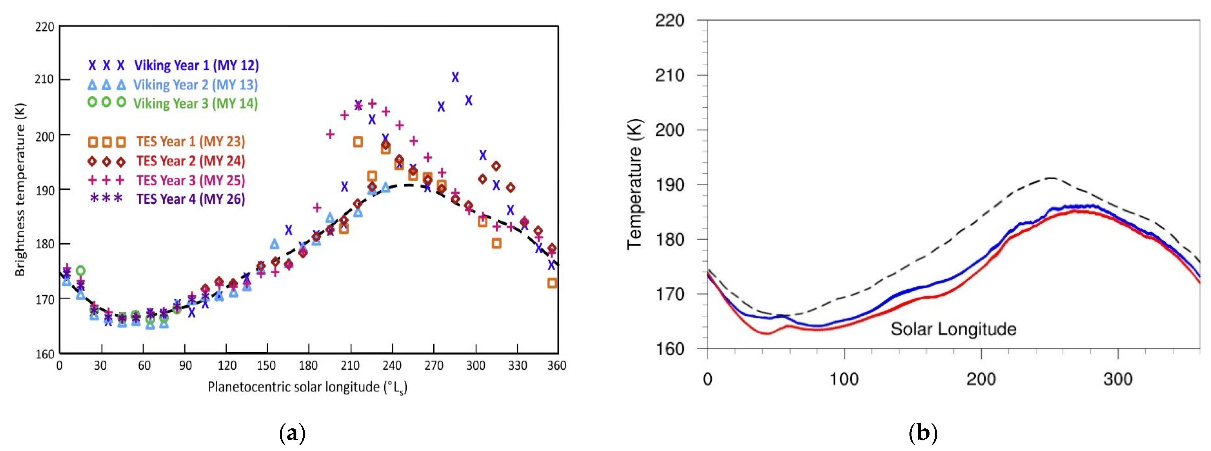
3.1. Temporal Distribution

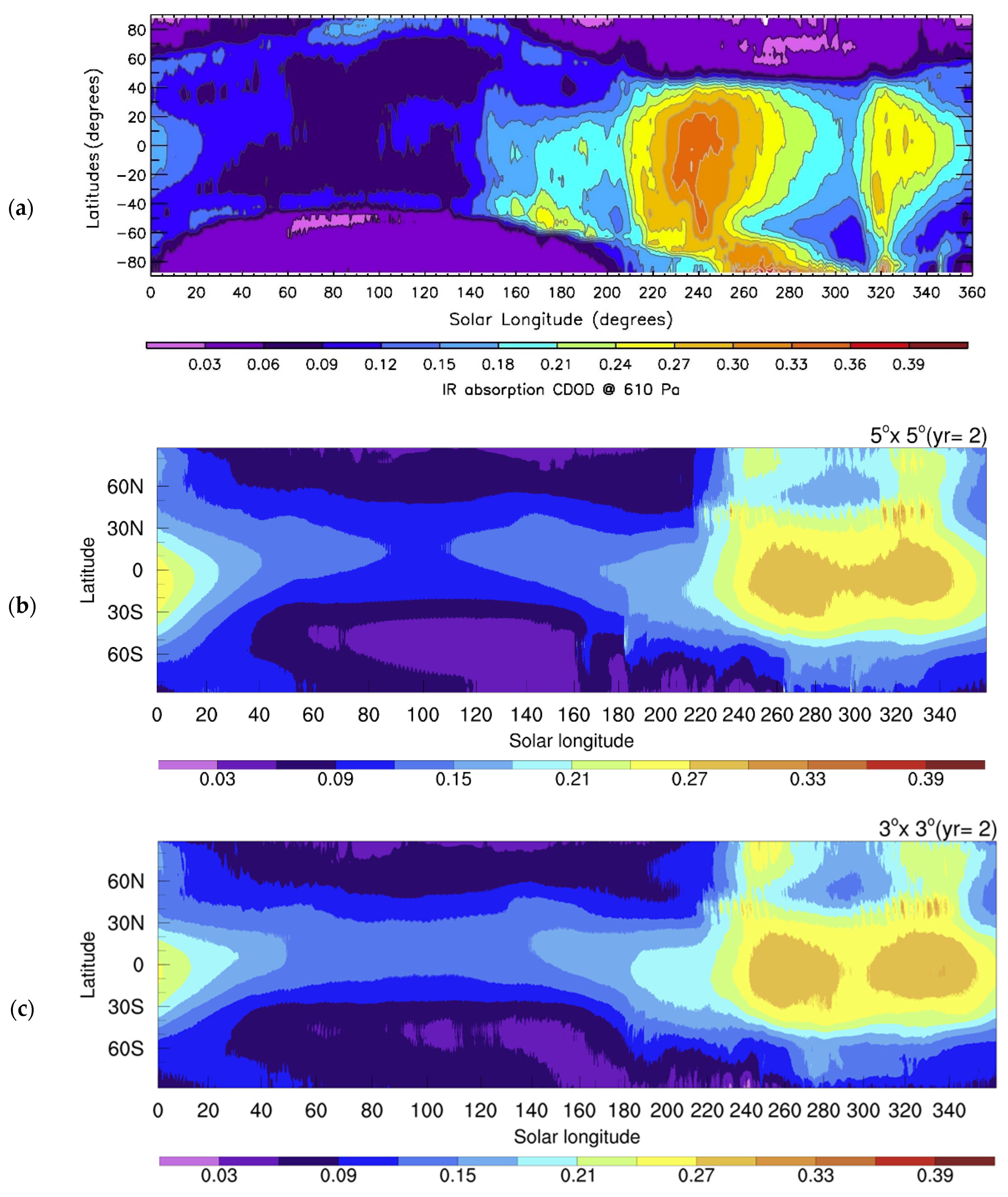
3.1.1. Column Dust Optical Depth

We tuned the dust-lifting parameters (discussed in Section 2.2) such that the simulated dust cycle in the 3° × 3° (HR) and 5° × 5° (SR) experiments were similar and were consistent with that from observations (Figure 2a). To achieve this goal, we conducted a series of sensitivity experiments by tuning the parameters α_N and α_D. Finally, in HR, we determined the parameters to be α_N = 0.17 × 10⁻⁴ and α_D = 0.4 × 10⁻⁹. In SR, we had α_N = 3.5 × 10⁻⁴ and α_D = 0.4 × 10⁻⁹.

The time series of the simulated zonal-mean column dust optical depth are shown in Figure 2b,c. Both HR and SR showed a similar pattern of annual variation in optical depth as in the observation (Figure 2a), and the magnitude of the optical depth was also similar in both simulations. The primary dust-lifting period is in the second half of the Martian year, with two peaks near Ls 240° and Ls 320°. During the first half of the year, airborne dust is rare.

3.1.2. Time Series of Dust Lifting

Given that the magnitude and annual variation in the column dust optical depth in the two simulations were similar, we examined if the characteristics of dust lifting were also similar. The corresponding time series of dust lifting by wind stress and dust devils are shown in Figure 3. Although we used a lower α_N in the HR simulation, the model generally produced a larger wind-stress dust lifting, especially in the Hellas Basin and the Olympus regions. In the HR case, there was a significant amount of dust lifting during northern spring and summer over the southern cap-edge region (Figure 3c), while in the SR case, dust lifting was lesser and mainly in the periods around Sol 120 and Sol 360 (Figure 3a). In the Olympus Mons region, there was continuous dust lifting during the first half of year in the HR case (Figure 3c) while there was no dust lifting in the SR case. In the dust season after Sol 400, the prominent dust-lifting activities in the northern mid-latitude region (Figure 3a,c) in both simulations were similar in both magnitude and pattern.

For dust lifting by dust devils, we set the same α_D parameters in the two simulations with different horizontal resolutions, and the time series (Figure 3b,d) showed that dust lifting by dust devils in the two cases was indeed similar. These results suggest that the simulation of dust lifting by dust devils was not significantly affected by model resolution.

The Viking Infrared Thermal Mapper 15-μm channel brightness temperature observations (IRTM T15) provide extensive spatial and temporal coverage of the Martian atmospheric temperature. The 15-μm channel was designed so that these temperatures would be a representative temperature of a deep layer of atmosphere centered at 50 Pa (~25 km). It is possible to directly synthesize T15 from the TES radiance observations. Wilson et al. [21] pointed out that by convolving the model temperature profiles with the weighting function of the IRTM channel, a good approximation can be achieved.

By using the IRTM weighting function, we calculated the global mean T15 from the two sets of simulation results and obtained the annual variations in the temperature (Figure 4). The black dashed line in Figure 4a shows the ‘climatological background’, which was effectively the global T15 curves with storm peaks removed, giving a hypothetical year with no major storms [22]. We can see when major storms were present in this year, the T15 value had a more obvious peak during the northern autumn, while the T15 value in other seasons was almost coincident with the background value. Figure 4b is our simulated T15. We can see that the T15 temperature in the HR case (blue curve) was in general slightly higher than that of the SR case (red curve), while the overall trend of the two curves in the whole year was the same. The T15 curve had its minimum value in the Martian spring and the maximum value in the Martian autumn. Compared with the Viking and TES observations, our simulated results were similar to the climatological background, although about 5 K lower.

3.2. Horizontal Distributions

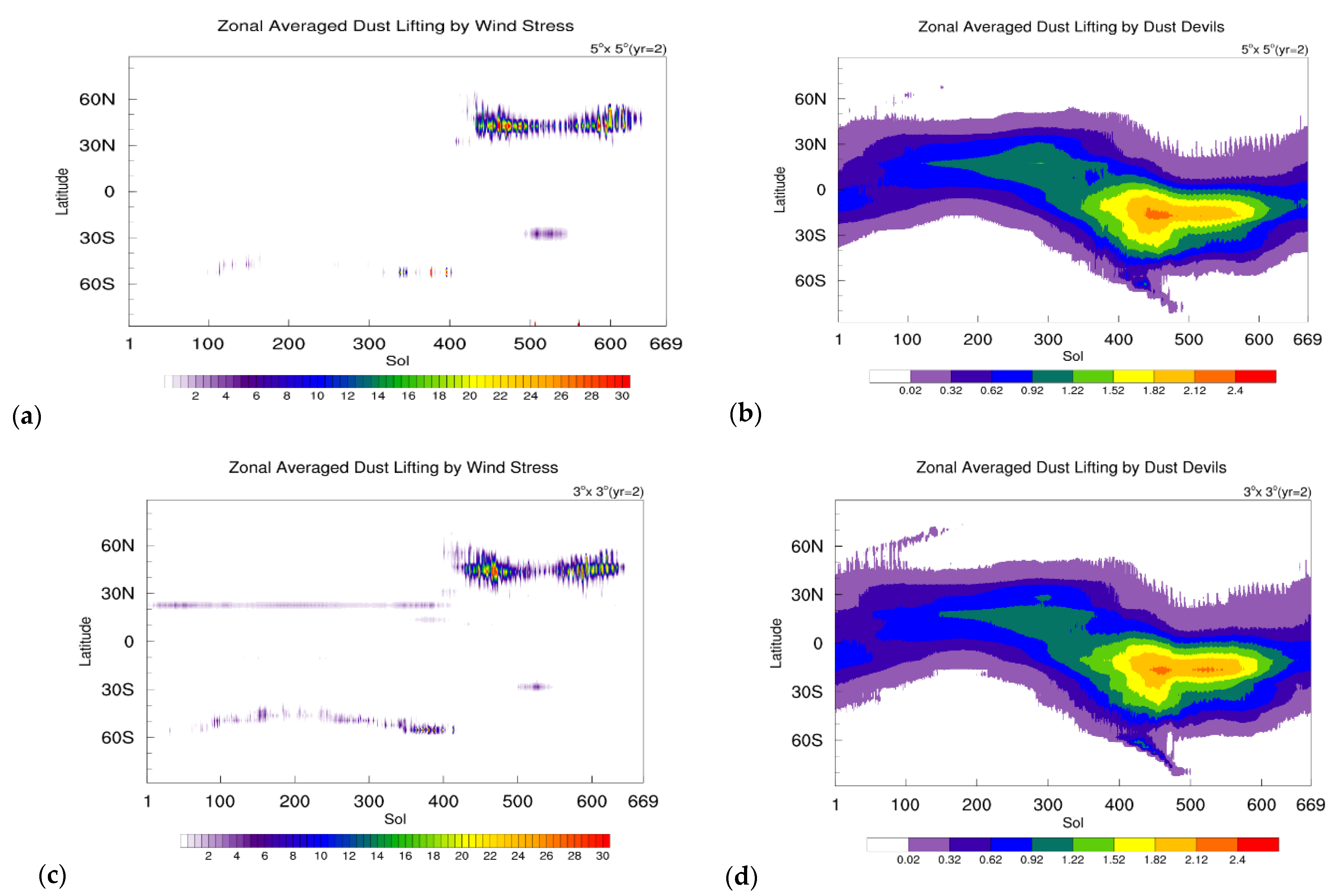
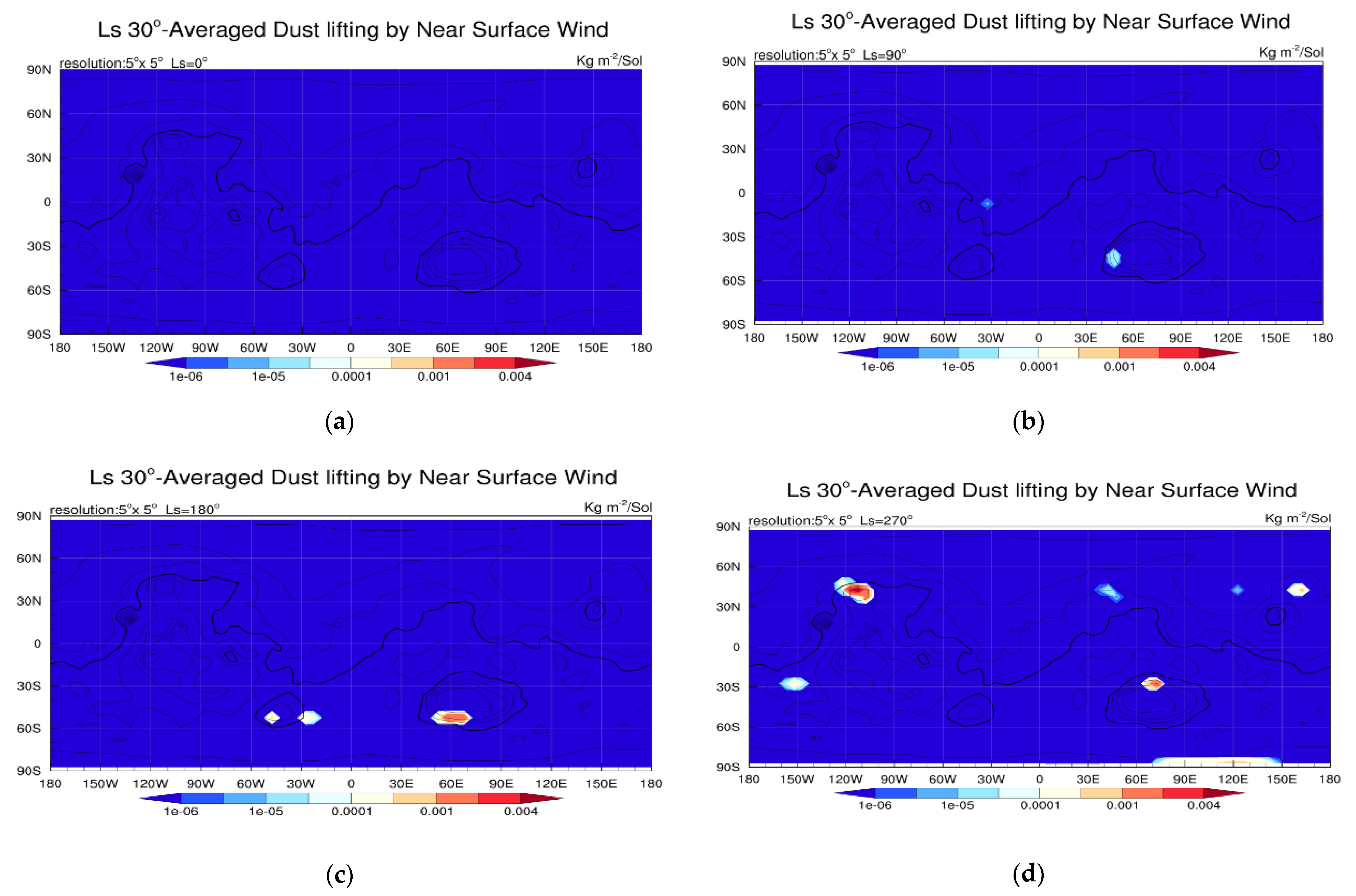
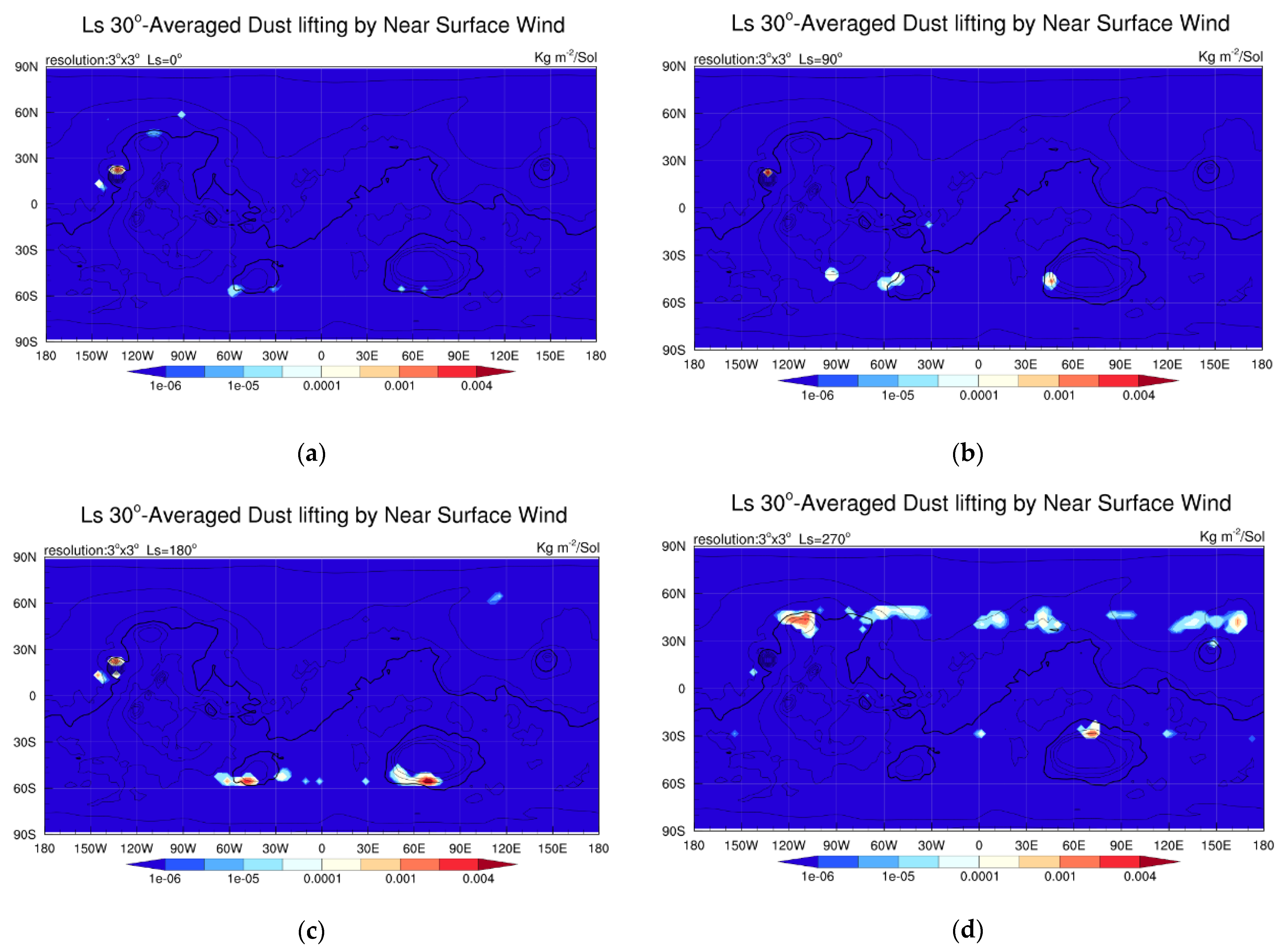
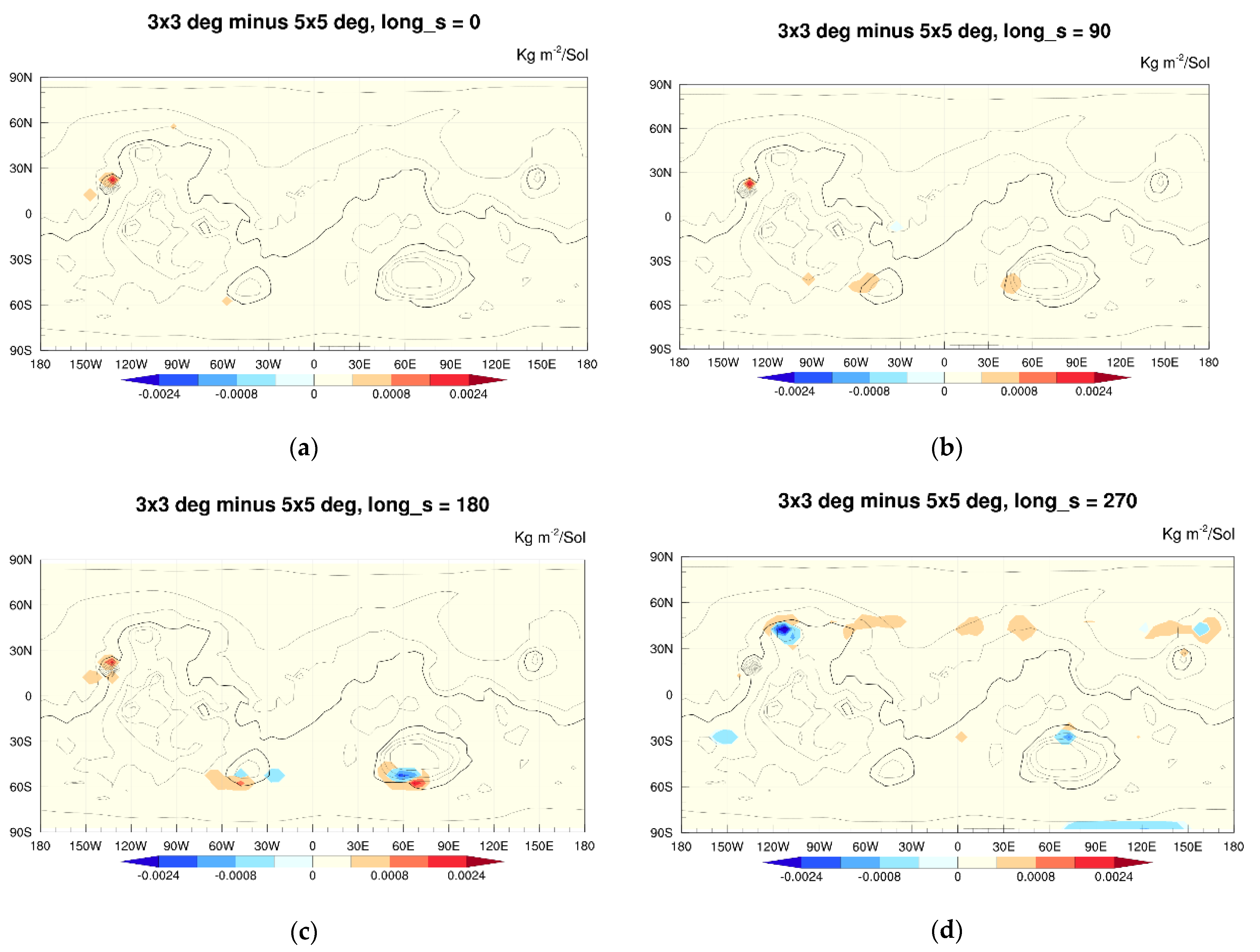
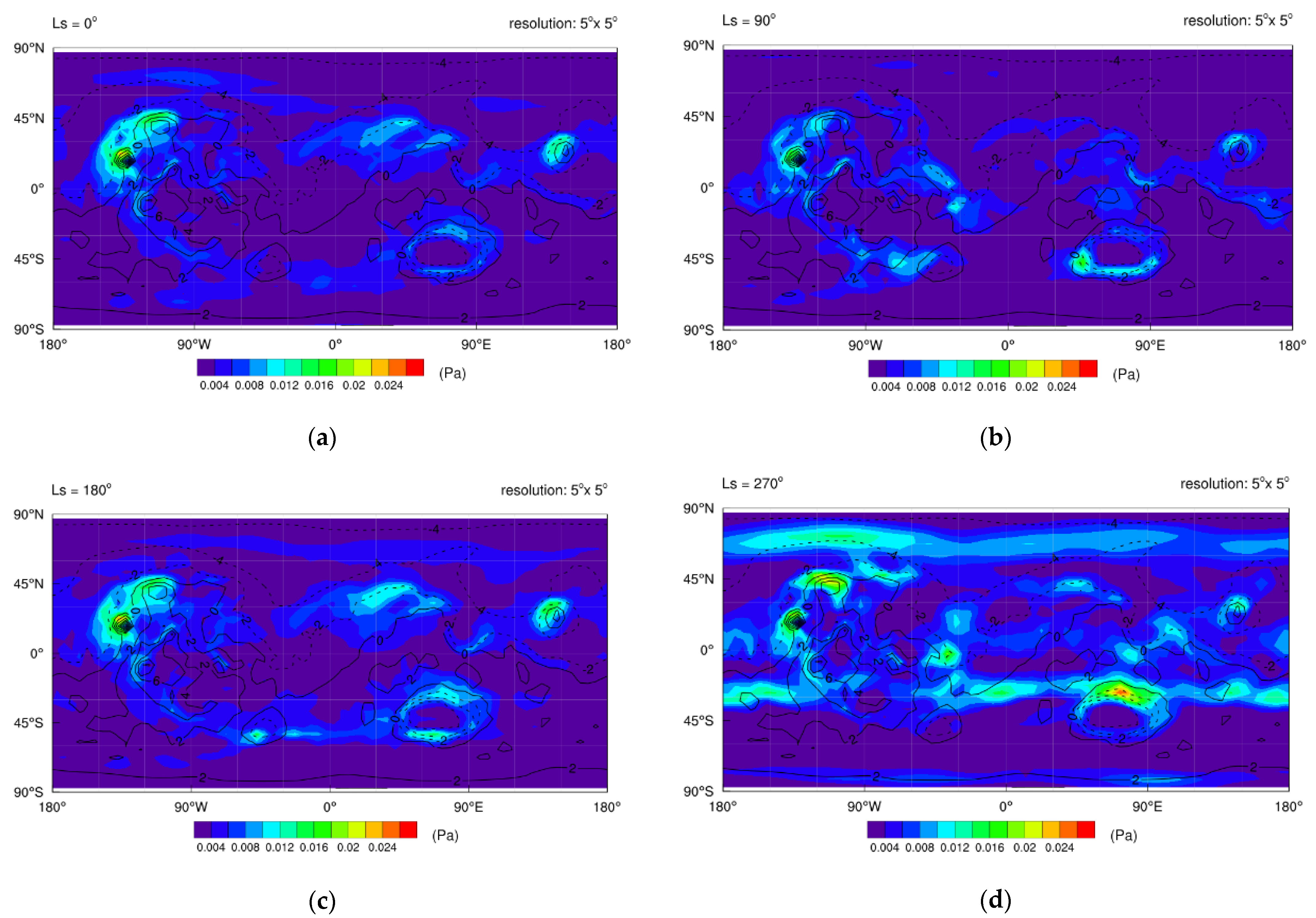
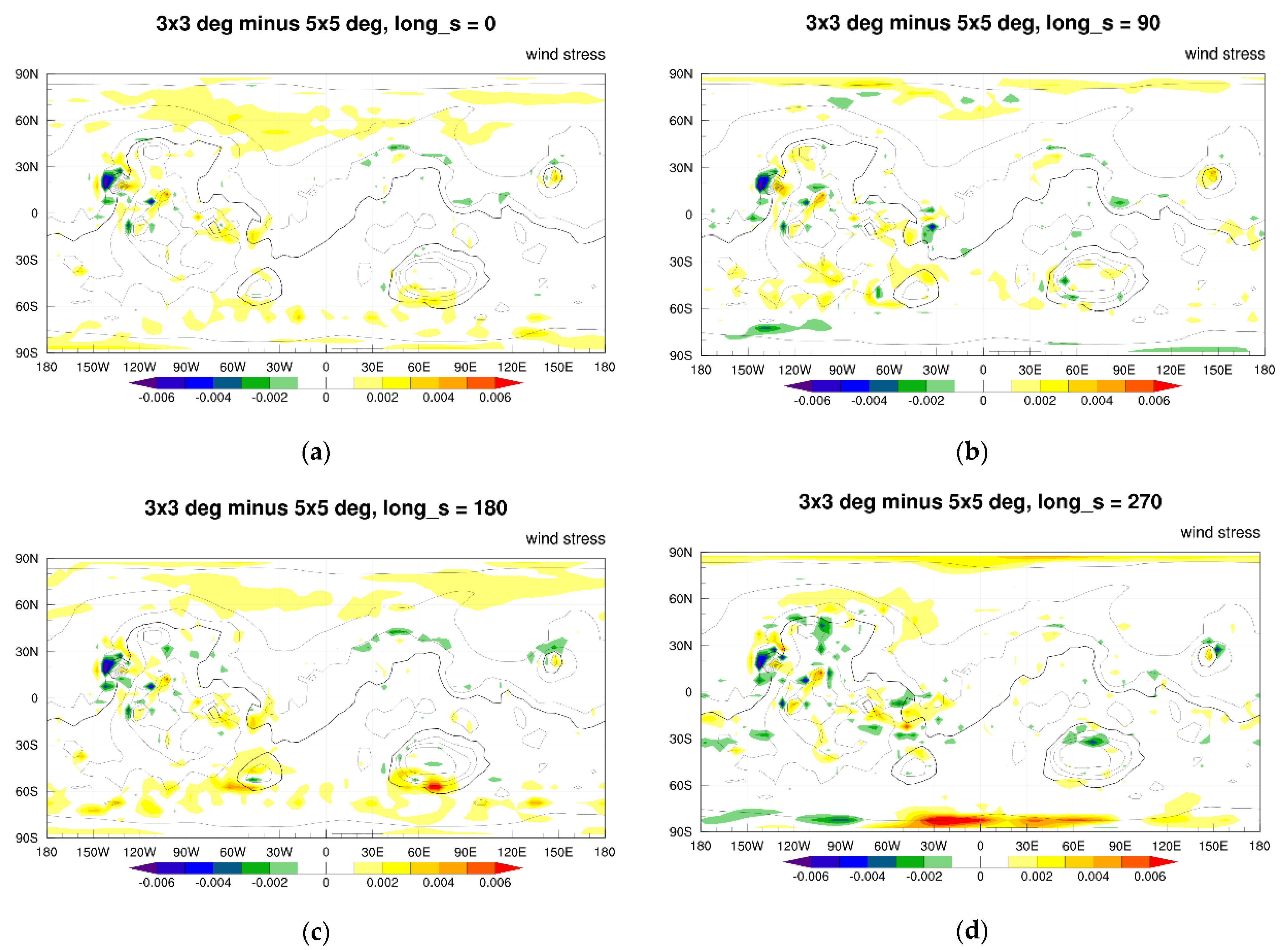
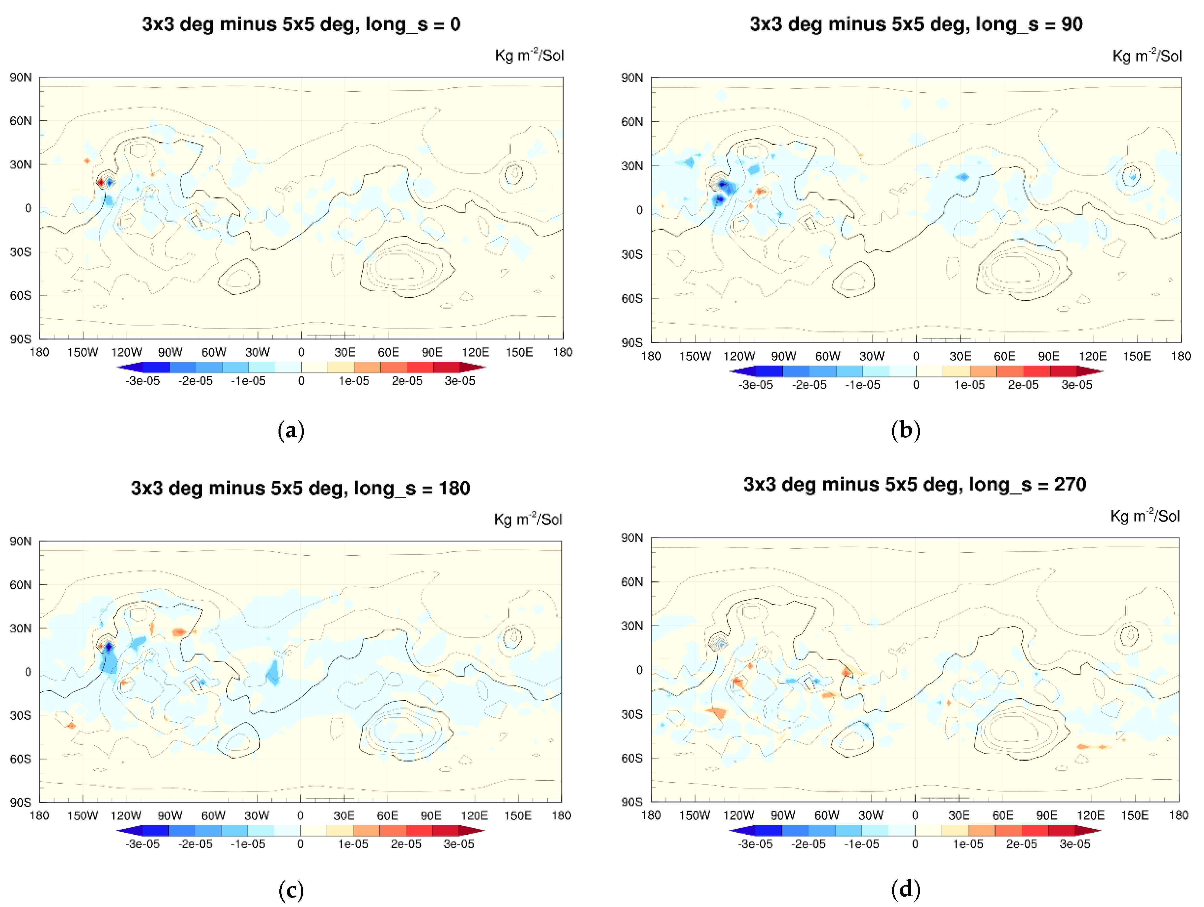
3.2.1. Dust Lifting by Wind Stress

Figure 5 and Figure 6 depict the horizontal distributions of wind-stress dust lifting in the four seasons. In general, the results of the two experiments showed a similar trend: around Ls = 0° and 90°, dust lifting by wind stress was less. Around Ls = 180° and 270°, dust lifting was substantially increased with a wider distribution. Around Ls = 0°, there was almost no dust lifting in the SR experiment, but in the HR experiment there was a small amount of dust lifting in the south of the Argyre basin and the Hellas basin, and a large amount of dust lifting was limited to the Olympus Mons region. Around Ls = 90°, there was a small amount of dust lifting in the west of the Hellas basin in the SR experiment. In the HR experiment, there was an additional small amount of dust lifting in the western part of the Argyre basin and the southern part of the Thaumasis Montes region, and substantial dust lifting was concentrated at the Olympus Mons region. Around Ls = 180°, both HR and SR had dust lifting in the southern part of the Hellas Basin and the Argyre basin. However, in HR there was an additional dust lifting area at the Olympus Mons region. At Ls = 270°, dust lifting was mainly in the north of the Hellas Basin around 45° S. In the SR experiment, the main dust lifting region in the northern hemisphere was located in the Alba Patera region. As the resolution was increased in HR, dust lifting in this region was reduced, which was different from the previous cases. The results showed that the overall dust lifting by wind stress in the HR experiment was a bit more than that in the SR experiment. In particular, at Ls = 0°, 90°, 180°, the Olympus Montes region showed obvious dust lifting, which was not captured in the SR experiment. However, there were still some exceptions. For example, at Ls = 270° dust lifting in the Alba Patera region decreased after increasing the horizontal resolution.

Figure 7 shows the differences in dust lifting by wind stress between the HR case and the SR case. We obtained the differences by interpolating the HR results on a 5° × 5° grid (same as SR) and then subtracted by the results of SR. From these figures, we can see that although the parameter α_N value used in HR was an order of magnitude smaller than that in SR, there were still some obvious positive values in most areas including the Olympus Mons region when Ls = 0°, 90°, and 180°, west of the Argyre basin and west of the Hellas basin when Ls = 90° and 180°, and the mid-latitude of the northern hemisphere when Ls = 270°.

Considering the simulated surface wind stress in Figure 8 and Figure 9, we found that the entire terrain of Olympus Mons in SR had a moderate value of wind stress (green color in Figure 8). On the other hand, moderate wind stress (green color) was basically around the Olympus Mons peak in HR, and the central peak region had a weaker wind stress (blue color). From this distribution, we inferred that under the low-resolution simulation of SR, the higher wind stress around Olympus Mons (as simulated in HR) and the low wind stress at the top was averaged to a lower value on the coarser grids, and the value did not reach the wind stress threshold for dust lifting. Therefore, in the SR case, there was no dust lifting in the Olympus Mons region.

Figure 10 shows the differences in surface wind stress. We can see there were some regions with positive difference, i.e., regions with greater wind stress in the HR case, such as the Olympus Mons, Elysium Mons, and Hellas basin regions. In the Olympus Mons region, we can see that wind stress in HR was greater around the peak (Figure 10) and was obviously less over the western side of the mountain. However, dust lifting in HR was only greater at the peak (Figure 7). The reason of this situation may be that the wind stress on the western side of the peak was very small and was less than the threshold wind stress in both SR and HR. Therefore, although the wind stress on the western side of the peak simulated in HR was less than that in the SR case, dust lifting by wind stress over there was not reduced in the HR case.

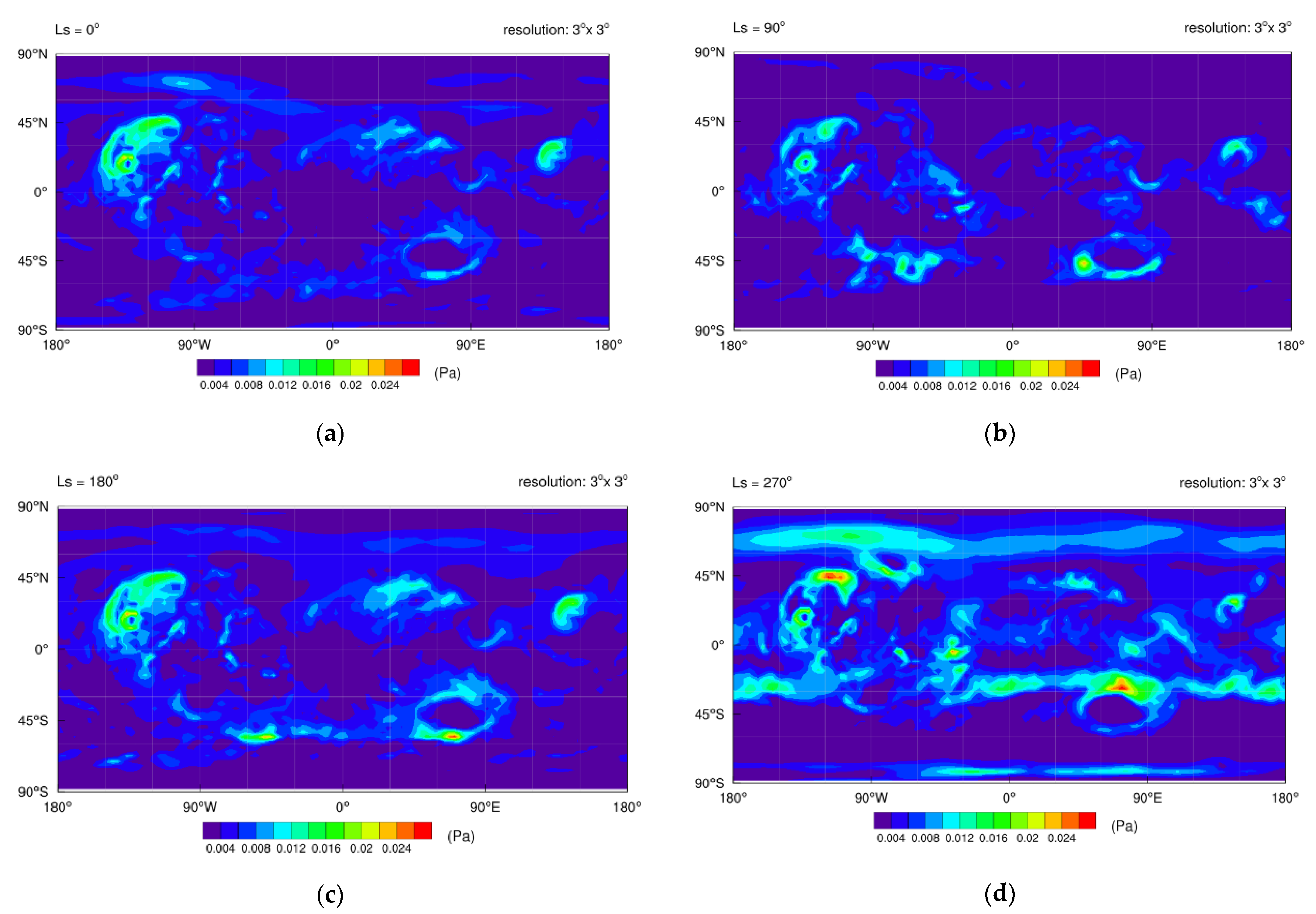
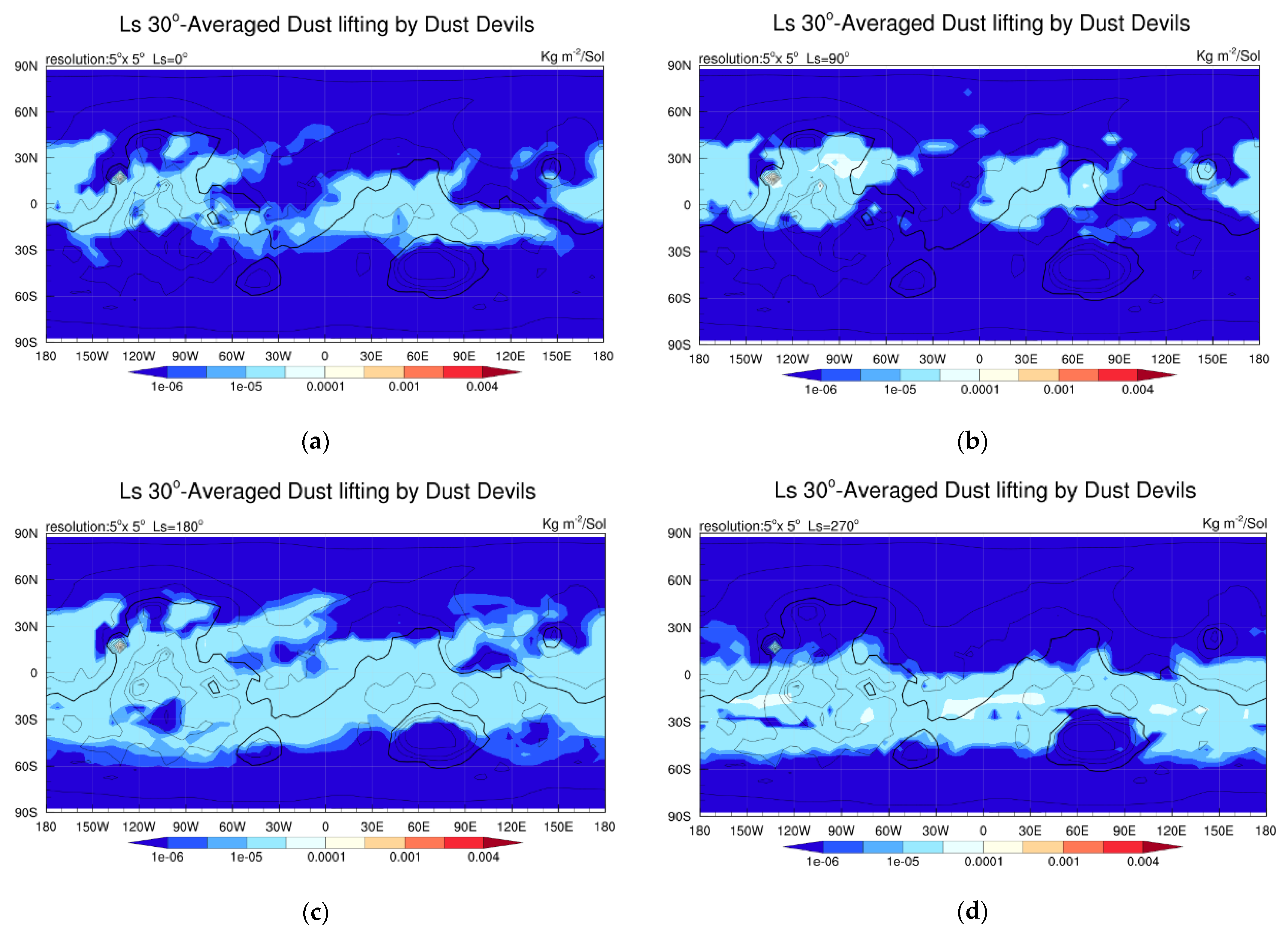
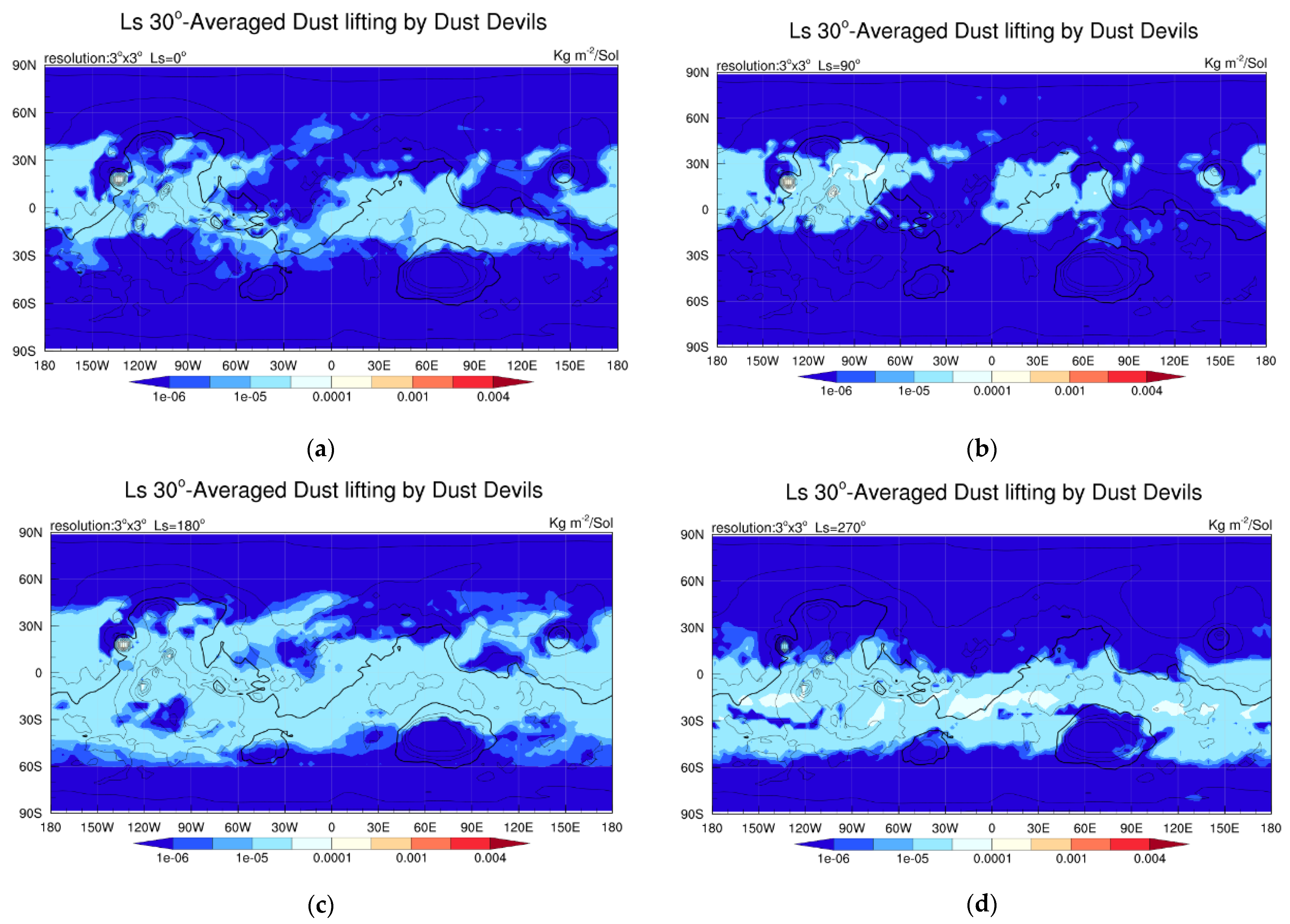
3.2.2. Dust Lifting by Dust Devils

Figure 11 and Figure 12 depict the distributions of dust lifting by dust devils in the four seasons. Comparing with Figure 5 and Figure 6, we can see the distribution of dust lifting by dust devils was relatively global, while the wind-stress dust lifting was basically concentrated in some regions. In general, the results of the two experiments showed a similar distribution pattern: around Ls = 0° and 90°, dust lifting was mainly in the middle and low latitudes of the northern hemisphere. Around Ls = 180°, dust lifting was mainly between 45° S and 45° N. Around Ls = 270°, dust lifting was mainly in the middle and low latitudes of the southern hemisphere. Figure 13 shows the differences in dust lifting by dust devils between the HR case and the SR case. We can see the impact of resolution was mainly significant over some particular terrains, such as in the Tharsis Montes and the Elysium Mons regions.

3.3. Vertical Distribution

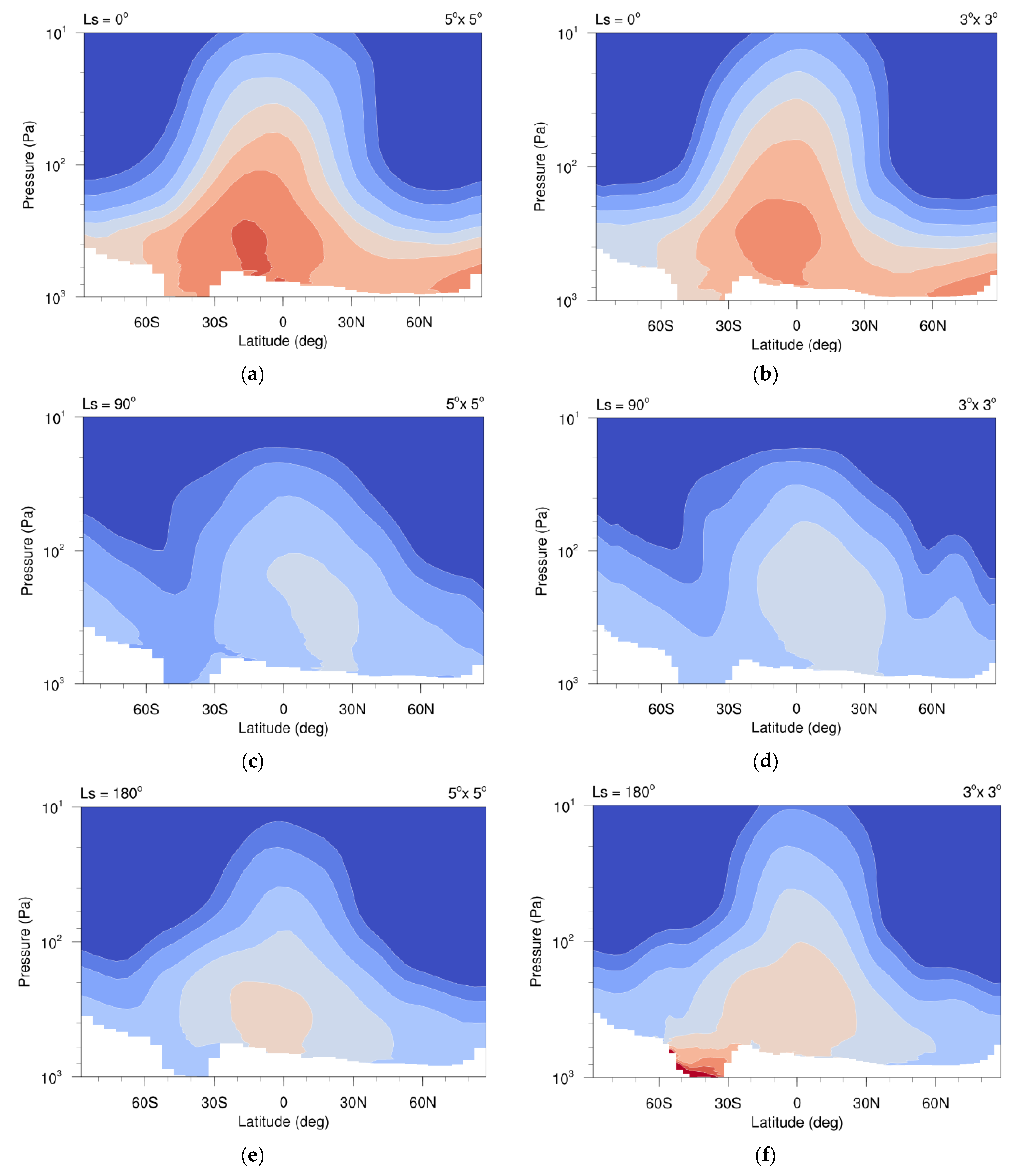
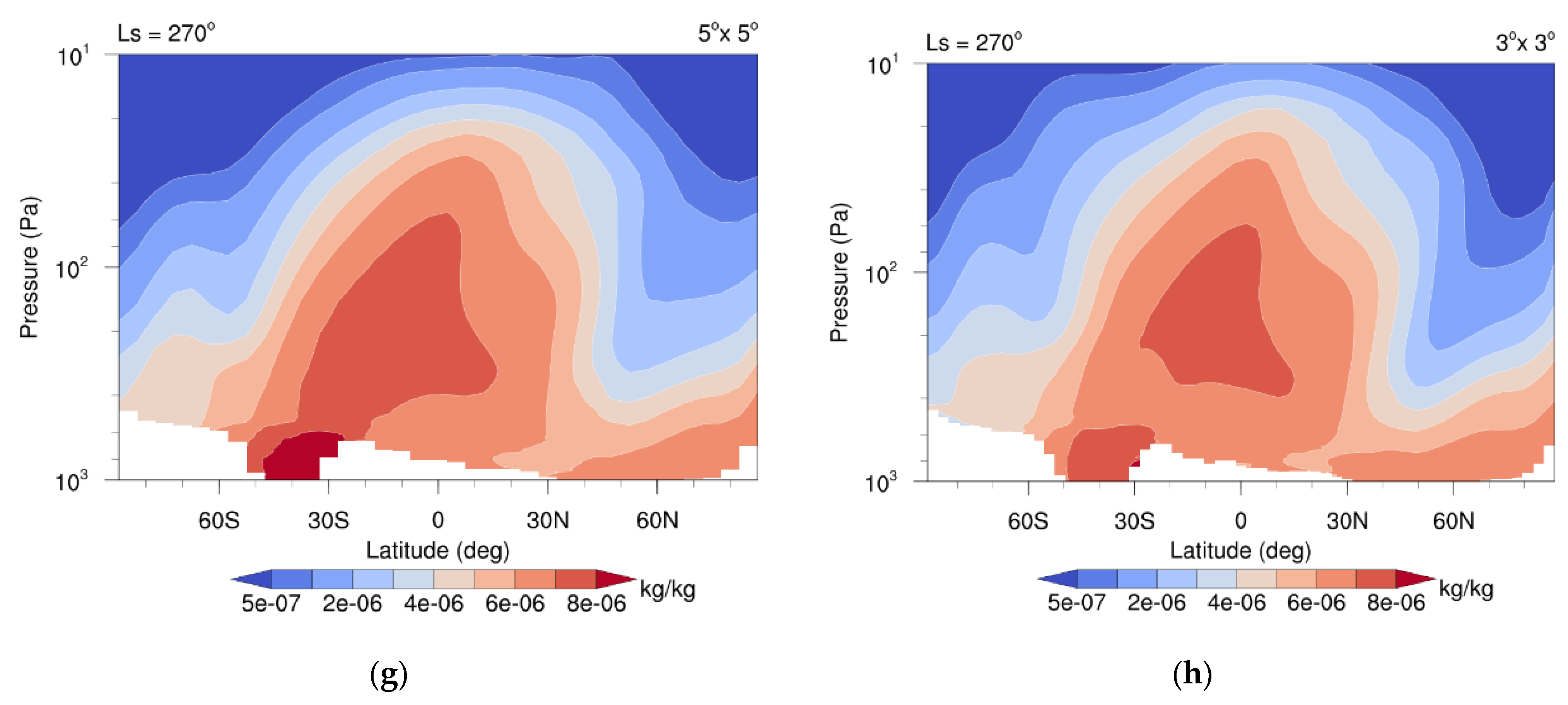
3.3.1. Dust Distribution

The vertical distribution of dust can greatly affect the vertical radiative balance and thus the atmospheric diabatic heating. The vertical transport of dust may also determine the horizontal transport and thus the horizontal spatial distribution of dust. Therefore, a full assessment and understanding of the seasonal and spatial variation in the vertical distribution of dust is important for fully characterizing the dust cycle.

Figure 14 shows the five-Sol-averaged vertical distribution of the dust-mixing ratio. We can see that dust was concentrated in low altitudes, and the dust-mixing ratio decreased as the altitude increased. There was a significant seasonal variation in the latitudinal position of the maximum dust-mixing ratio. Around Ls = 0°, the maximum was near the equator. Around the northern summer solstice (Ls = 90°), the position of the maximum was significantly moved to about 25° N. This indicates that the vertical distribution of dust was associated with the latitudinal position of maximum solar radiation.

Although the vertical resolution and dust particle sizes were the same in both the HR and SR simulations, there were still some differences in the vertical dust distribution. Around Ls = 180°, the maximum in the SR case was still near the equator. However, in the HR case, possibly due to the enhanced dust lifting over the abrupt terrain of the Hellas basin, the maximum moved to the south and the value obviously increase. Compared with SR, dust particles in HR could extend to a higher level of the troposphere (Figure 14f), possibly due to the stronger atmospheric circulation in the HR case. Around Ls = 270°, the maximums of SR and HR were rather different over the Hellas basin. Although the amount of dust in the Hellas basin region was relatively small in HR, the contours of the dust mixing ratio at the upper portion of the troposphere between 30° S and 60° S could extend to higher altitudes.

During the northern summer when Mars is near the aphelion, the dust-mixing ratio in the vertical profile was at the lowest value during the year (Figure 14c,d). During the northern winter solstice (Ls = 270°), the vertical dust mixing ratio was largest (Figure 14g,h), which means that the dust loading in the atmosphere was largest at this time. This is due to the increased global temperature of Mars near the perihelion, and so the atmospheric circulation is strengthened.

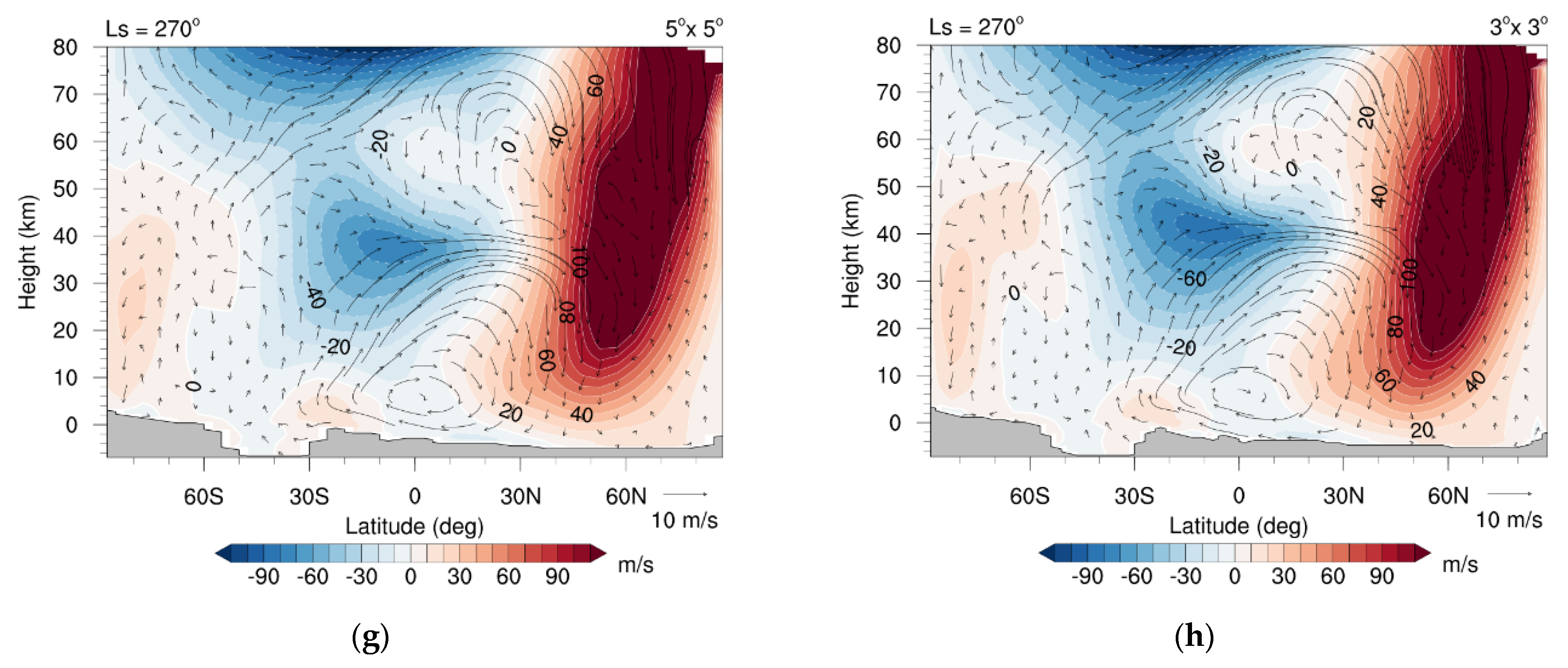
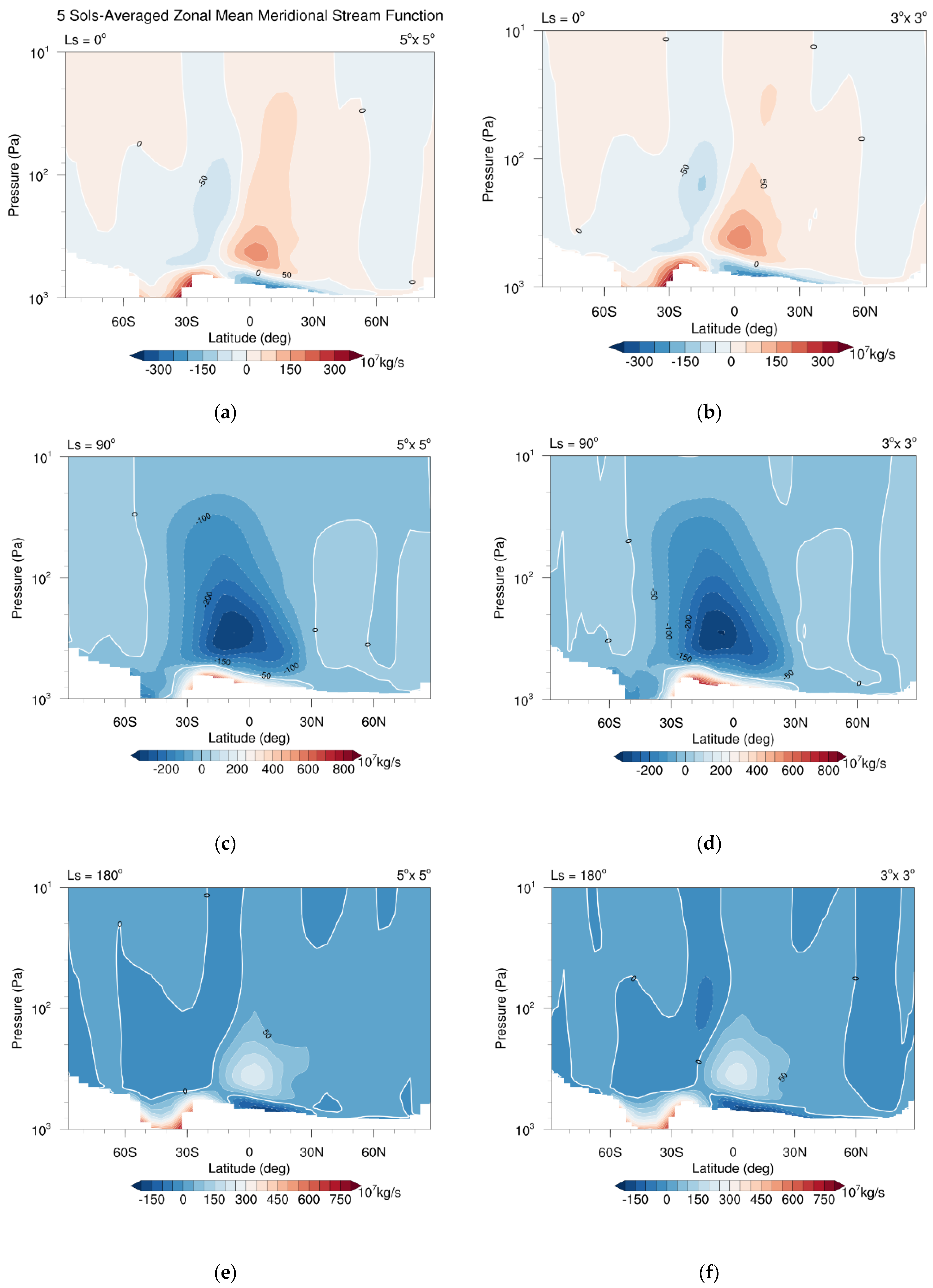
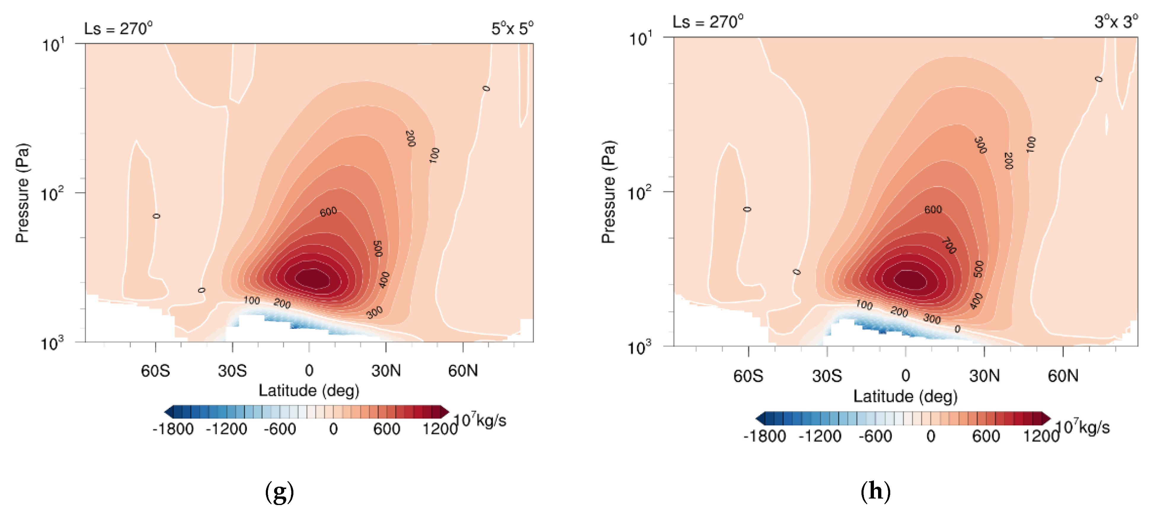
3.3.2. Dynamic Field

To study the effect of model resolution on the circulation, we first considered the vertical distribution of zonal wind (Figure 15). Around Ls = 0° and Ls = 180°, westerly wind (red color) is prevalent in the high latitudes of both hemispheres, while there is a center of strong easterly wind (blue color) at the upper troposphere near the equator. Around Ls = 90°, there is a center of strong westerly wind in the high latitudes of the southern hemisphere. On the other side there is a center of weak westerly wind in high latitudes of the northern hemisphere, and in low latitudes there are three centers of weak easterly wind in the vertical direction. Around Ls = 270°, the high latitudes of the northern hemisphere have a center of strong westerly wind, and the high latitudes of the southern hemisphere have a weak westerly wind, and there are two centers of strong easterly wind at high altitudes over the low-latitude region. Comparing the simulation results of SR and HR in Figure 15, we can see that the general pattern did not change a lot with resolution, but there were some subtle differences between the HR and SR simulations. Around Ls = 0°, the high-altitude easterly wind center in the HR was more widely distributed in both the vertical and north-south directions. Each hemisphere had a maximum of westerly wind speed over the middle- and high-latitude regions in SR, but the two maximum values were both separated into two high-wind centers in HR. Around Ls = 90°, the northern westerly wind center in the HR case separated into two centers, and the southern westerly wind center had a higher maximum value than that in the SR case. Around Ls = 180°, the westerly and easterly winds in the HR case seemed weaker than that in the SR case. Around Ls = 270°, the westerly wind in the northern hemisphere weakens and the easterly wind center in the low latitudes increased.

The mean meridional circulation plays a vital role in the cross-equatorial transport of dust. Its intensity can be represented by the meridional stream function (MSF), which can be evaluated by the following equation:

$$\psi \left(\varphi ,p\right)=\frac{2\pi R}{g}cos\varphi {{\displaystyle \int }}_{ps}^p\overline{v}\left(\varphi ,p\right)dp$$

(5)

where ψ (ϕ, p) is the MSF at pressure level p and latitude ϕ. R is the radius of Mars (3390 km), and g is the gravity acceleration on Mars (3.727 m s⁻²). $\overline{v}$ is the zonal-mean meridional wind. The MSF is an intuitive physical quantity that gives a quantitative description of the zonal-mean meridional circulation. The contours of ψ reflect the stream lines, and the gradient of ψ is proportional to the velocity $\overline{v}$.

Figure 16 shows the simulated MSFs in different seasons. The Hadley circulation is largely confined in the troposphere below 10 Pa and is mainly driven by the temperature difference related to the imbalance of radiation energy, and thus has a strong seasonal variability. At the spring and autumn equinoxes, the northern and southern hemispheres are dominated by two Hadley cells. Due to the eccentricity of the orbit, absorbed solar radiation in the two hemispheres is not symmetrical, and so the two Hadley cells in the northern and southern hemispheres are asymmetric. The cell in the northern winter is stronger, with an ascending branch near the equator and the circulation extends to the southern hemisphere. In general, in the northern summer and the southern summer, the two Hadley cells develop into a single and strong Hadley cell connecting the two hemispheres, and so reflecting the circulation of air mass between the summer and the winter hemispheres.

Comparing the results of SR and HR (Figure 16), we found that there was generally not much difference in the pattern and intensity of the MSF. However, it appeared that the top of the Hadley cell could develop to a higher altitude in the HR case around Ls = 270° (c.f. Figure 16g,h).

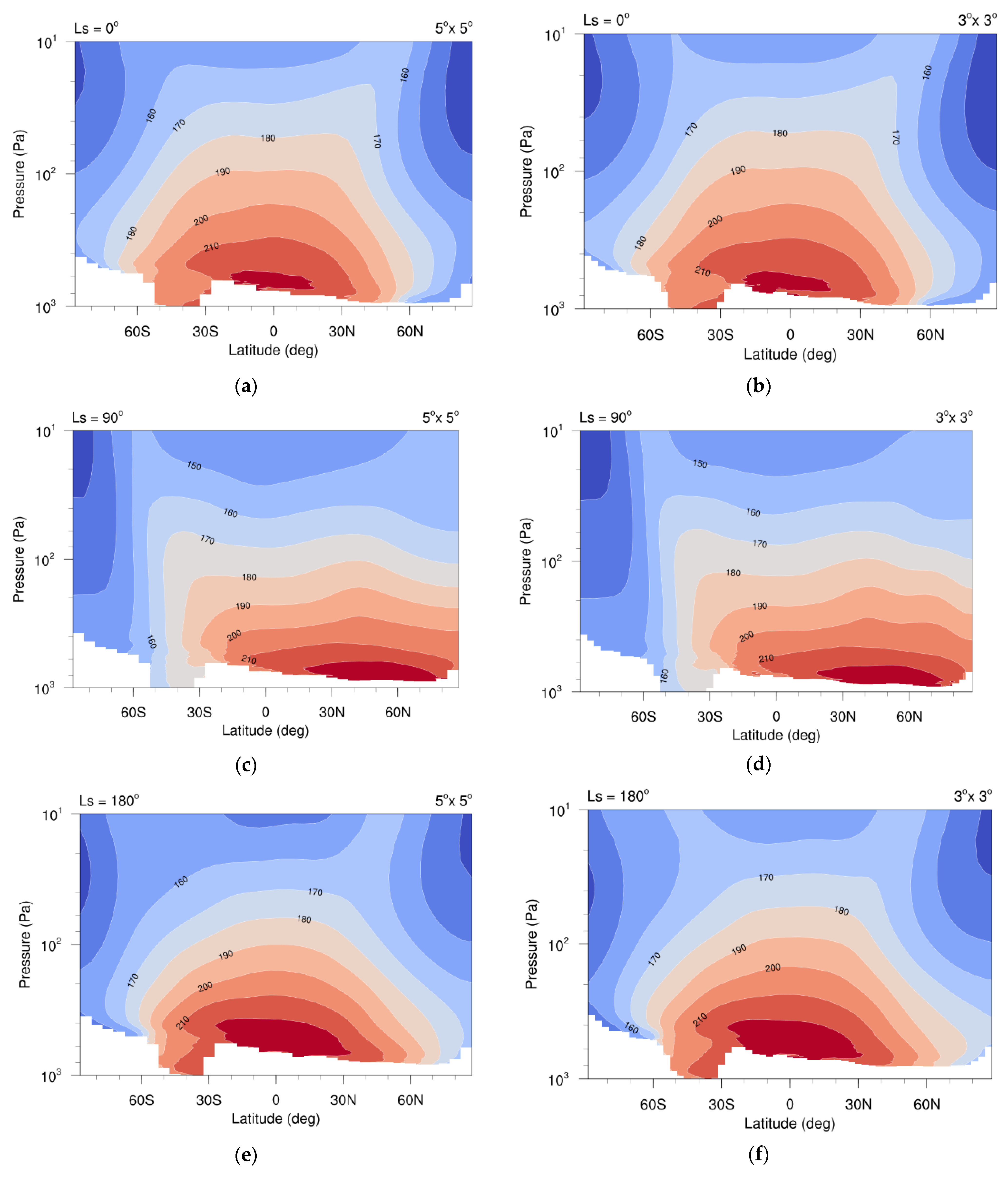
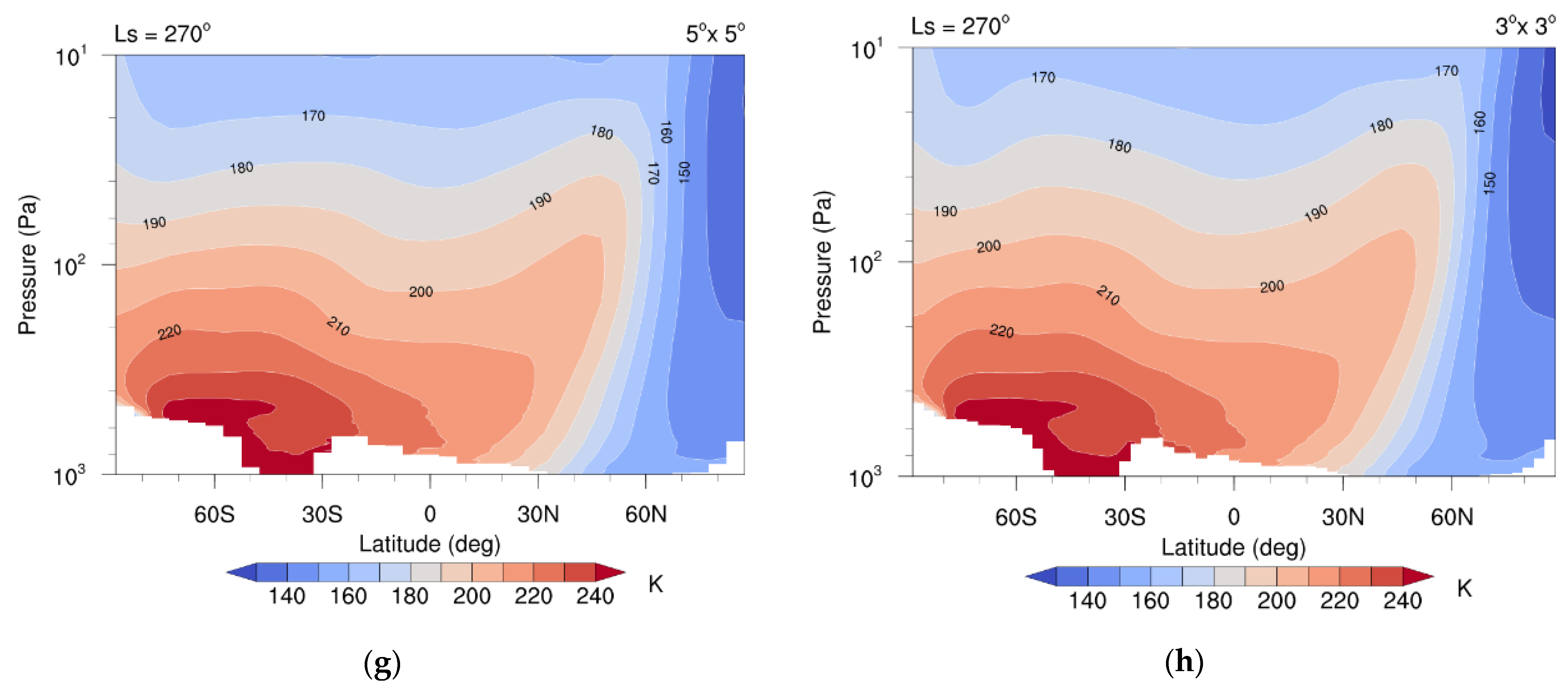
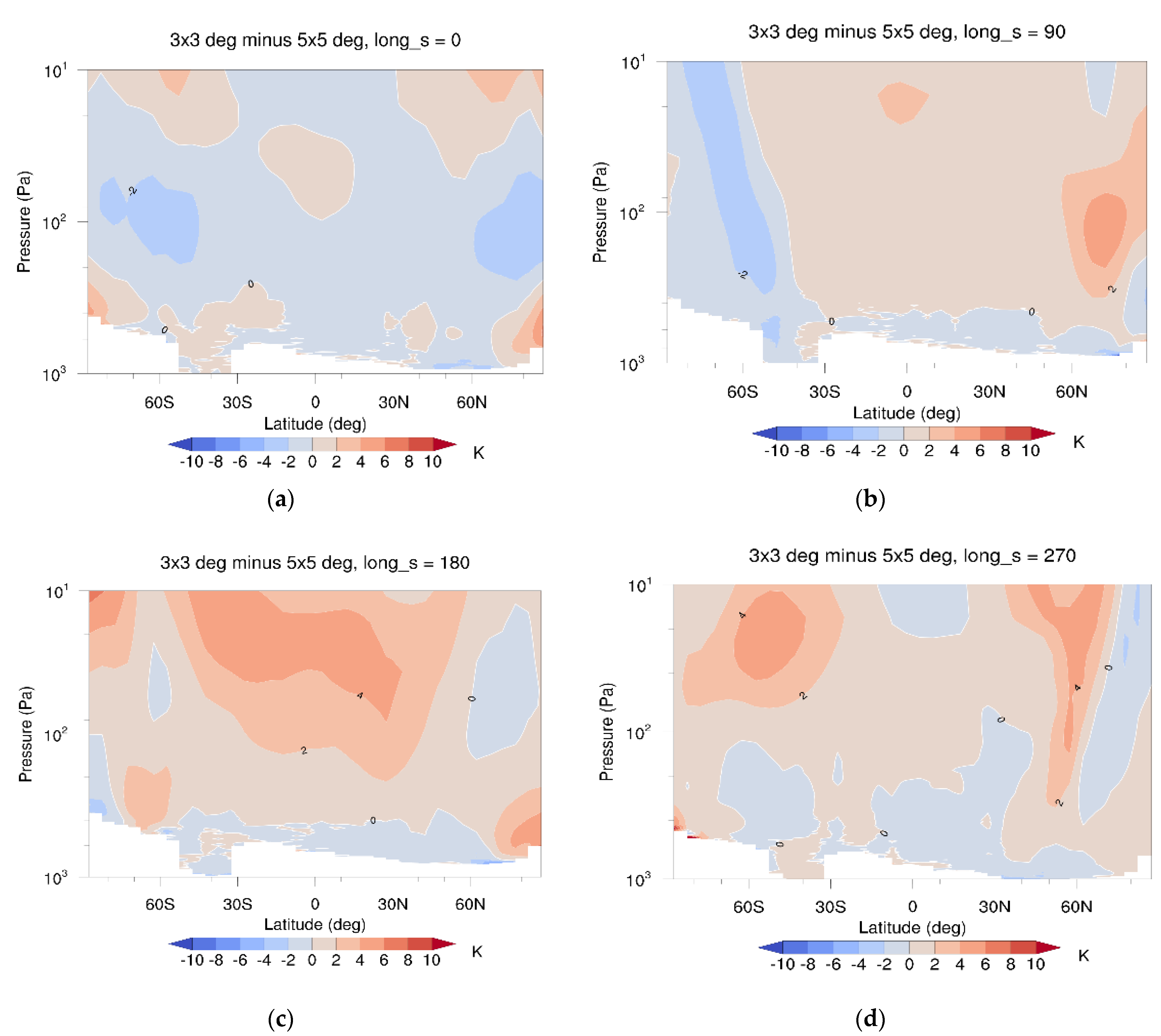
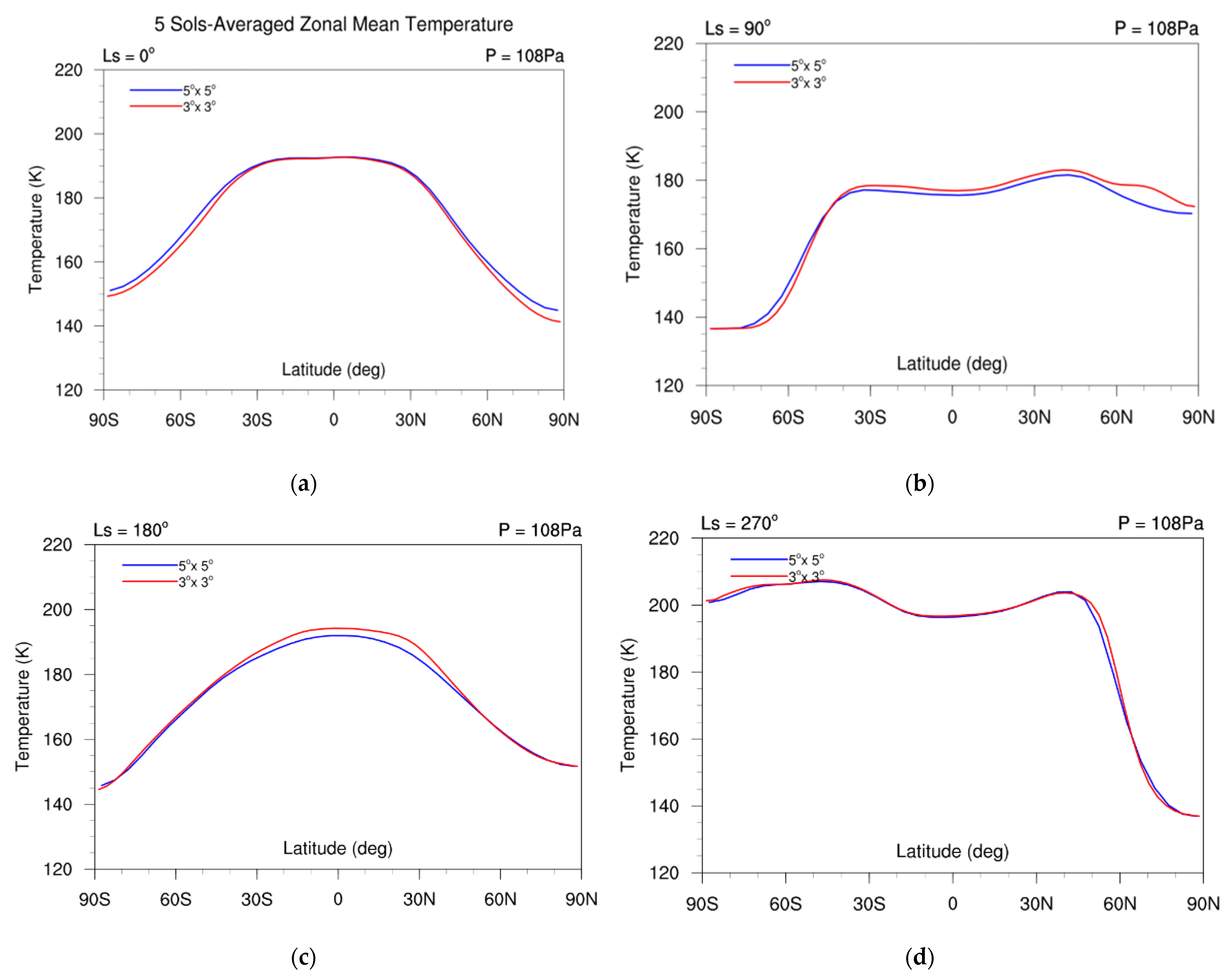
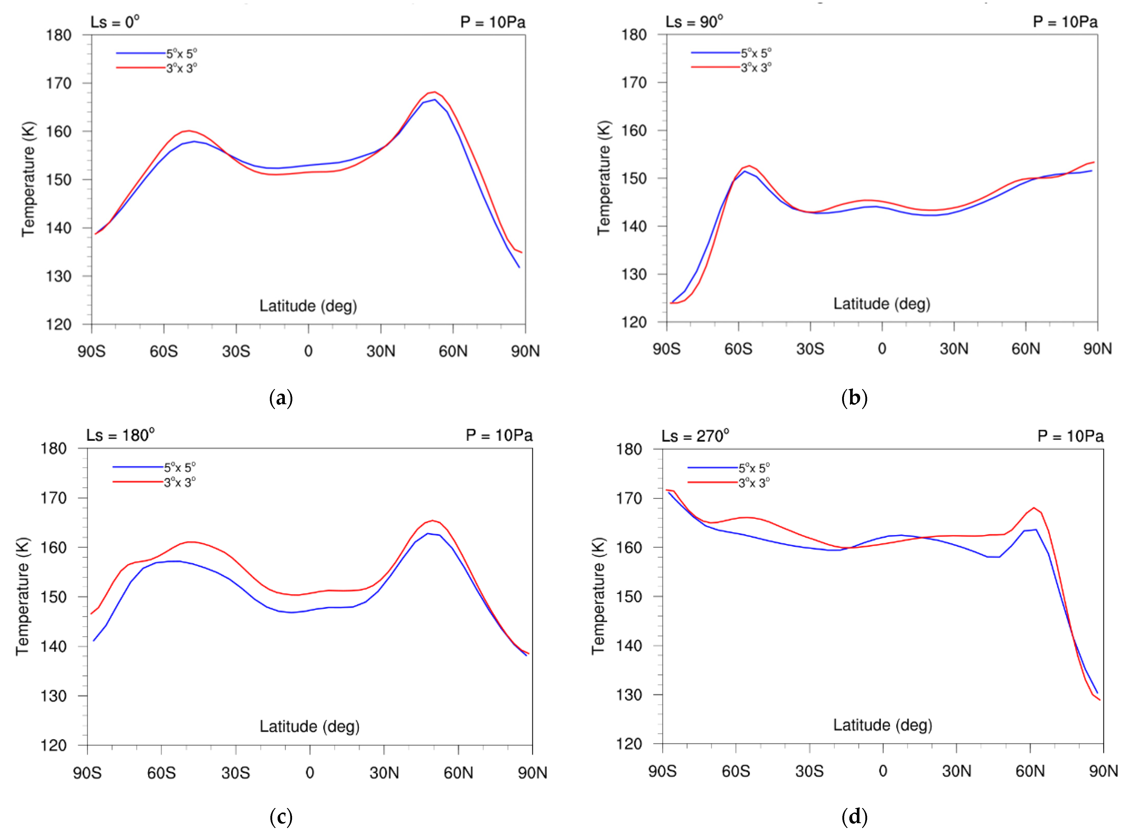
3.3.3. Thermal Field

Figure 17 shows the vertical temperature distribution in the four seasons. It can be seen from the figures that the thermal structure could change significantly with season and latitude. The position of the maximum value was generally related to the latitude of the maximum solar radiation. Comparing the northern summer solstice (Ls = 90°, Figure 17c,d) and winter solstice (Ls = 270°, Figure 17g,h), we can see that at the same pressure level over low- and mid-latitudes, the atmospheric temperature around Ls = 270° could be 20 K higher than the temperature around Ls = 90°.

Figure 17 shows that the zonal-mean temperature field in the HR case was not significantly different from that in the SR case, and the simulation results were generally consistent with the Mars Climate Sounder (MCS) thermal observations (e.g., [23]). Despite the similar distribution, there were indeed some temperature differences between HR and SR, as shown in Figure 18. Around Ls = 0° (Figure 18a), the simulated temperature in HR was higher over the polar region and was lower in the high latitudes near the 100 Pa height. The negative temperature difference near the north and south poles could be related to the vertical dust distribution in Figure 14. Around Ls = 0°, the dust-mixing ratio near the surface of the northern polar region was higher in SR, while it was lower in HR. The difference in dust mixing ratio was negatively correlated to the temperature difference. This may be due to the blocking of some solar radiation by the dust near the ground, thus reducing the downward solar radiation at the surface, and thus reducing the near-surface temperature.

Around Ls = 90° (Figure 18b), the simulated temperature over the high latitudes of the southern hemisphere was lower in HR, while the temperature at the high latitudes of the northern hemisphere was warmer in HR, corresponding to the small bulge at ~70° N in the HR case (Figure 14d).

Around Ls = 180° (Figure 18c), an obvious positive difference could be seen between 100 Pa and 10 Pa over the region of 60° S–60° N. From Figure 14, we can see that more dust could be found in the upper troposphere in the HR simulation, corresponding to the positive temperature difference in Figure 18. More dust in the upper part of the troposphere may absorb more solar radiation and so generate a stronger heating in the atmosphere.

Around Ls = 270° (Figure 18d), the distribution of dust could also be used to analyze the difference in temperature fields. The positive temperature difference in the upper troposphere at 60° S corresponded to the bulge in the dust-mixing ratio contour in HR. The negative temperature difference near the surface at 60° S corresponded to the larger dust-mixing ratio above the Hellas basin in the SR case. Again, this is because the low-level dust may reduce the downward solar radiation at the surface, while the dust in the upper troposphere may contribute radiative heating to the atmosphere.

To further analyze the difference in the vertical distribution of temperature in the two simulations, we considered the zonal-mean temperature at a level of 108 Pa (following Toigo et al. [12]), which was at an altitude of about 17 km. From Figure 19 we can see that when Ls = 0°, the temperature at this altitude level was slightly lower in the HR case, especially in the mid and high latitudes. Around Ls = 180°, the simulated temperature in the HR case was a bit higher. Around Ls = 90°, there was no significant bias in temperature, and the two curves of temperature crossed at a latitude of 45° S. Around Ls = 270°, there was only a little variation in temperature in the two simulations. We can see that in the mid and high latitudes, the temperature decreased with the increase in latitude, and the slope of the curve was slightly steeper in the HR case, which means that the temperature zonal gradient in the mid and high latitudes was larger in the HR case.

Figure 20 shows the zonal-mean temperature curve in the middle atmosphere at a level of 10 Pa, roughly at a height of 42 km (again following Toigo et al. [12]). Comparing with the results at the level of 108 Pa (Figure 19), we can see that the difference between SR and HR was generally greater at a higher altitude. This indicates that, in the vertical direction, the model resolution had a weaker effect on the atmospheric simulation in the lower troposphere. Obviously, the temperature maximum became warmer, and the minimum became cooler in the HR case. Around Ls = 0° and Ls = 180°, there was a maximum in each hemisphere, and the extreme value in the northern hemisphere was always larger. This further illustrates the asymmetry of the circulation in the two hemispheres. Similar to that in the 108 Pa level, the HR case showed stronger temperature gradients in the mid and high latitudes.

It is worth mentioning that although Toigo et al. [12] used a different dust scenario and looked at slightly different resolutions, the patterns of the curves in Figure 19 and Figure 20 are similar to what they showed, i.e., they also saw a steep gradient in the north of ~60 N (south of ~60 S for Ls = 90). However, in the middle atmosphere (10 Pa) around Ls = 270°, the temperature in the mid to high northern latitudes region was lower in their high-resolution simulation. On the contrary, the corresponding temperature was higher for the high-resolution simulation in the present study (Figure 20d).

4. Conclusions

In this study, we investigated the impact of model horizontal resolution on Martian climate simulations by using the Mars GCM MarsWRF. The vertical grid was the same in all simulations. In general, running a model with higher resolution is preferred but the computing resources involved should be much larger, and so simulations with Mars GCMs are usually run at a relatively low resolution such as 5° × 5°. The results of this study indicated some possible differences in the simulation results when running the model at a lower resolution. In the two simulations with different horizontal resolutions (HR and SR), we used an interactive dust scheme to parameterize the dust-lifting processes and adjusted the tunable dust-lifting parameters α_D and α_N so that the annual variation in column dust optical depth in the two sets of simulations were similar and consistent with observations. The time series of this quantity is usually used to evaluate the performance of a Mars GCM in simulating the dust climate of Mars. Given that the time series of optical depth were similar in the two simulations, we investigated in which aspects the model resolution will make differences when simulating the climate of Mars with a Mars GCM

Considering the temporal distribution, we found that there was only a slight difference in the pattern of seasonal variation in dust-devils dust lifting, i.e., the simulation of dust lifting by dust devils was not significantly affected by model resolution. On the other hand, there were some significant differences in the pattern of annual variation in wind-stress dust lifting. The differences were mainly in the Olympus Mons region and the southern cap-edge region. In the first half of the year, there were some dust-lifting activities in these two regions in the HR case, while it was absent in the SR case.

When looking at the horizontal distribution, we have the following findings: (1) In the HR simulation, dust lifting by wind stress was generally more in the northern mid-latitude and the southern cap-edge regions. (2) The impact of resolution on the simulation of dust lifting by dust devils was only significant in the regions with complicated terrain. Some differences were found in the Tharsis Montes and Elysium Mons regions.

From the vertical cross-sections of climate fields, we found that: (1) The vertical distribution of dust was generally consistent with the vertical temperature field. Dust distribution in the lower levels was negatively correlated with the temperature field, while the dust distribution in the upper troposphere was positively correlated with the temperature field. (2) Comparing the vertical cross-sections of zonal wind, we found that the resolution could affect the zonal wind speed in the upper troposphere. At Ls = 0° and Ls = 90°, the HR case simulated two high westerly wind centers at high latitudes of the northern hemisphere, while there was only one center simulated in the SR case. (3) When the Hadley circulation intensifies in the northern autumn near the perihelion, the top branch of the Hadley cell in HR may extend to a higher altitude, thus resulting in a higher extent of dust in the HR simulation. (4) The analysis of the temperature contours at different altitudes indicated that the effect of the model resolution in the simulated vertical distribution could be greater at higher altitudes.

Overall, our results suggest that changing from 5° × 5° to 3° × 3° with interactive dust had only a limited effect on the simulation of the Martian climate. A significant difference was mainly found in some special terrains, such as the Olympus Mons, Hellas Basin, and southern cap-edge regions. Therefore, when the study region has a complicated topography, high horizontal resolution should be used to obtain more accurate results. In regions with relatively flat terrain, such as the Tianwen-1 landing site at the Utopia Planitia, we obtained almost similar results by using standard resolution with less computing resources occupied. However, in any case when the simulation of the vertical distribution is important, simulation with a higher horizontal resolution is recommended.

References

1. Newman, C.E.; Lewis, S.R.; Read, P.L.; Forget, F. Modeling the Martian dust cycle 2. Multiannual radiatively active dust transport simulations. J. Geophys. Res. Planets 2002, 107, 5123. [Google Scholar] [CrossRef] [Green Version]
2. Basu, S.; Wilson, J.; Richardson, M.; Ingersoll, A. Simulation of spontaneous and variable global dust storms with the GFDL Mars GCM. J. Geophys. Res. 2006, 111, E09004. [Google Scholar] [CrossRef]
3. Newman, C.E.; Richardson, M.I. The impact of surface dust source exhaustion on the Martian dust cycle, dust storms and inter-annual variability, as simulated by the MarsWRF General Circulation Model. Icarus 2015, 257, 47–87. [Google Scholar] [CrossRef]
4. Gebhardt, C.; Abuelgasim, A.; Fonseca, R.M.; Martín-Torres, J.; Zorzano, M.P. Characterizing dust radiation feedback and refining the horizontal resolution of the marswrf model down to 0.5 degree. J. Geophys. Res. Planets 2021, 126, e2020JE006672. [Google Scholar] [CrossRef]
5. Rafkin, S.C.R. A positive radiative-dynamic feedback mechanism for the maintenance and growth of Martian dust storms. J. Geophys. Res. 2009, 114, E01009. [Google Scholar] [CrossRef] [Green Version]
6. Neary, L.; Daerden, F. The GEM-Mars General Circulation Model for Mars: Description and Evaluation. Icarus 2018, 300, 458–476. [Google Scholar] [CrossRef]
7. Bertrand, T.; Wilson, R.J.; Kahre, M.A.; Urata, R.; Kling, A. Simulation of the 2018 global dust storm on Mars using the NASA Ames Mars GCM: A multitracer approach. J. Geophys. Res. Planets 2020, 125, e2019JE006122. [Google Scholar] [CrossRef] [Green Version]
8. Kieffer, H.; Jakosky, B.M.; Snyder, C.W.; Mathews, M.S. (Eds.) Mars; University of Arizona Press: Tucson, AZ, USA, 1992. [Google Scholar]
9. Pollack, J.B.; Leovy, C.B.; Mintz, Y.H.; van Camp, W. Winds on Mars during the Viking season: Predictions based on a general circulation model with topography. Geophys. Res. Lett. 1976, 3, 479–482. [Google Scholar] [CrossRef]
10. Forget, F.; Hourdin, F.; Fournier, R.; Hourdin, C.; Talagrand, O.; Collins, M.; Lewis, S.R.; Read, P.L.; Huot, J.P. Improved general circulation models of the Martian atmosphere from the surface to above 80 km. J. Geophys. Res. 1999, 104, 24155–24176. [Google Scholar] [CrossRef]
11. Richardson, M.I.; Toigo, A.D.; Newman, C.E. PlanetWRF: A general purpose, local to global numerical model for planetary atmospheric and climate dynamics. J. Geophys. Res. 2007, 112, E09001. [Google Scholar] [CrossRef]
12. Toigo, A.D.; Lee, C.; Newman, C.E.; Richardson, M.I. The impact of resolution on the dynamics of the martian global atmosphere: Varying resolution studies with the marswrf gcm. Icarus 2012, 221, 276–288. [Google Scholar] [CrossRef]
13. Gebhardt, C.; Abuelgasim, A.; Fonseca, R.M.; Martín-Torres, J.; Zorzano, M.-P. Fully interactive and refined resolution simulations of the martian dust cycle by the marswrf model. J. Geophys. Res. Planets 2020, 125, e2019JE006253. [Google Scholar] [CrossRef]
14. Skamarock, W.C.; Klemp, J.B. A time-split non-hydrostatic atmospheric model for Weather Research and Forecasting applications. J. Comput. Phys. 2008, 227, 3465–3485. [Google Scholar] [CrossRef]
15. Chow, K.-C.; Chan, K.-I.; Xiao, J. Dust activity over the Hellas basin of Mars during the period of southern spring equinox. Icarus 2018, 311, 306–316. [Google Scholar] [CrossRef]
16. Chow, K.C.; Xiao, J.; Wang, Y.M. Simulation of dust activities in the southern high latitudes of Mars. Planet. Space Sci. 2022, 217, 105492. [Google Scholar] [CrossRef]
17. Xiao, J.; Chow, K.-C.; Chang, K.-I. Dynamical processes of dust lifting in the northern mid-latitude region of Mars during the dust storm season. Icarus 2019, 317, 94–103. [Google Scholar] [CrossRef]
18. Wang, Y.M.; Chow, K.C.; Xiao, J.; Wong, C.F. Effect of dust particle size on the climate of Mars. Planet. Space Sci. 2021, 208, 105346. [Google Scholar] [CrossRef]
19. Madeleine, J.B.; Forget, F.; Millour, E.; Montabone, L.; Wolff, M.J. Revisiting the radiative impact of dust on Mars using the LMD Global Climate Model. J. Geophys. Res. Planets 2011, 116, E11. [Google Scholar] [CrossRef] [Green Version]
20. Montabone, L.; Forget, F.; Millour, E.; Wilson, R.; Lewis, S.; Cantor, B.; Smith, M.J.I. Eight-year climatology of dust optical depth on Mars. Icarus 2015, 252, 65–95. [Google Scholar] [CrossRef] [Green Version]
21. Wilson, R.J.; Richardson, M.I. The martian atmosphere during the viking mission, i: Infrared measurements of atmospheric temperatures revisited. Icarus 2000, 145, 555–579. [Google Scholar] [CrossRef]
22. Basu, S.; Richardson, M.I.; Wilson, R.J. Simulation of the Martian dust cycle with the GFDL Mars GCM. J. Geophys. Res. 2004, 109, E11006. [Google Scholar] [CrossRef] [Green Version]
23. McCleese, D.J.; Heavens, N.G.; Schofield, J.T.; Abdou, W.A.; Bandfield, J.L.; Calcutt, S.B.; Irwin, P.G.; Kass, D.M.; Kleinböhl, A.; Lewis, S.R.; et al. Structure and dynamics of the Martian lower and middle atmosphere as observed by the Mars Climate Sounder: Seasonal variations in zonal mean temperature, dust, and water ice aerosols. J. Geophys. Res. 2010, 115, E12016. [Google Scholar] [CrossRef]
Figure 1. (a) Mars global topography (m) in the SR simulation (resolution 5° × 5°). (b) Topography (m) in the HR simulation (resolution 3° × 3°). (c) Map of Mars with major regions labeled. (https://attic.gsfc.nasa.gov/mola/images/topo_labeled.jpg, accessed on 15 May 2022).
Atmosphere 13 01736 g001
Figure 2. (a) Seasonal variation in zonal-mean column dust optical depth normalized to 600 Pa reconstructed from observational data (Montabone et al. 2015 [20]), obtained by averaging the observational data over eight Martian years (MY24–MY33, excluding the years with planet-encircling dust storm activity in MY25 and MY28). The data was downloaded from the website of the Laboratoire de Météorologie Dynamique du CNRS (LMD). (b)Time series of zonal-mean column dust optical depth in the SR simulation (resolution 5° × 5°) and (c) the HR simulation (resolution 3° × 3°), normalized at the surface level (700 Pa).
Atmosphere 13 01736 g002
Figure 3. (a) Time series of zonal-mean dust lifting (kg m−2 Sol−1) by surface wind stress in the SR simulation (resolution 5° × 5°). (b) Time series of zonal-mean dust lifting by dust devils in the SR simulation (resolution 5° × 5°). (c,d) are similar to (a,d) but for the HR simulation (resolution 3° × 3°).
Atmosphere 13 01736 g003
Figure 4. (a) Global mean T15 temperature curves for seven Martian years from the Infrared Thermal Mapper (IRTM) instruments on board the Viking Orbiters and the thermal emission spectrometer (TES) instrument on board the Mars Global Surveyor (MGS) spacecraft (colored dots). The black dashed curve represents the climatological background. This figure is from Newman and Richardson (2015), adapted with permission from the publisher. (b) The corresponding global mean T15 temperatures from the SR simulation (the red curve) and the HR case (blue curve). The black dashed curve represents the climatological background in (a).
Atmosphere 13 01736 g004
Figure 5. Global distribution of dust lifting (shading, kg m−2 Sol−1) by surface wind stress, averaged for 30° Ls around (a) Ls = 0°, (b) 90°, (c) 180° and (d) 270° in the SR simulation (resolution 5° × 5°). Contours depict the topography. x- and y-axes show the longitudes and latitudes, respectively.
Atmosphere 13 01736 g005
Figure 6. As in Figure 5 but for the HR simulation (resolution 3° × 3°).
Atmosphere 13 01736 g006
Figure 7. Differences (HR minus SR) in global dust lifting (kg m−2 Sol−1) by surface wind stress at (a) Ls = 0°, (b) 90°, (c) 180°, and (d) 270°, averaged for a period of 30° Ls. Contours depict the topography. x- and y-axes show the longitudes and latitudes, respectively.
Atmosphere 13 01736 g007
Figure 8. Global distribution of surface wind stress (Pa), averaged for 30° Ls around (a) Ls = 0°, (b) 90°, (c) 180°, and (d) 270° in the SR simulation (resolution 5° × 5°). Contours depict the topography. x- and y-axes show the longitudes and latitudes, respectively.
Atmosphere 13 01736 g008
Figure 9. As in Figure 8 but for the HR simulation (resolution 3° × 3°).
Atmosphere 13 01736 g009
Figure 10. Differences (HR minus SR) in global surface wind stress (Pa) at (a) Ls = 0°, (b) 90°, (c) 180°, and (d) 270°, averaged for a period of 30° Ls. Contours depict the topography. x- and y-axes show the longitudes and latitudes, respectively.
Atmosphere 13 01736 g010
Figure 11. Global distribution of dust lifting (kg m−2 Sol−1) by dust devils, averaged for 30° Ls around (a) Ls = 0°, (b) 90°, (c) 180°, and (d) 270° in the SR simulation (resolution 5° × 5°). Contours depict the topography. x- and y-axes show the longitudes and latitudes, respectively.
Atmosphere 13 01736 g011
Figure 12. As in Figure 11 but for the HR simulation (resolution 3° × 3°).
Atmosphere 13 01736 g012
Figure 13. Differences (HR minus SR) in global dust lifting (kg m−2 Sol−1) by dust devils at (a) Ls = 0°, (b) 90°, (c) 180°, and (d) 270°, averaged for a period of 30° Ls. Contours depict the topography. x- and y-axes show the longitudes and latitudes, respectively.
Atmosphere 13 01736 g013
Figure 14. Vertical cross-section of five-Sol-averaged zonal-mean dust-mixing ratio (kg kg−1) around (a,b) Ls = 0°, (c,d) Ls = 90°, (e,f) Ls = 180°, and (g,h) Ls = 270° in the SR (left column) and the HR (right column) simulations.
Atmosphere 13 01736 g014aAtmosphere 13 01736 g014b
Figure 15. Vertical cross-section of five-Sol-averaged zonal-mean wind field (m s−1) around (a,b) Ls = 0°, (c,d) Ls = 90°, (e,f) Ls = 180°, and (g,h) Ls = 270° in the SR (left column) and the HR (right column) simulations. Westerly and easterly wind are shown in red and blue colors, respectively.
Atmosphere 13 01736 g015aAtmosphere 13 01736 g015b
Figure 16. Vertical slices of five-Sol-averaged meridional stream function around (a,b) Ls = 0°, (c,d) Ls = 90°, (e,f) Ls = 180°, and (g,h) Ls = 270° in the SR (left column) and the HR (right column) simulations.
Atmosphere 13 01736 g016aAtmosphere 13 01736 g016b
Figure 17. Vertical cross-section of five-Sol-averaged zonal-mean temperature (K) around (a,b) Ls = 0°,(c,d) Ls = 90°, (e,f) Ls = 180°, and (g,h) Ls = 270° in the SR (left column) and the HR (right column) simulations.
Atmosphere 13 01736 g017aAtmosphere 13 01736 g017b
Figure 18. Vertical cross-section of differences (HR minus SR) in five-Sol-averaged zonal-mean temperature (K) around (a) Ls = 0°, (b) Ls = 90°, (c) Ls = 180°, and (d) Ls = 270°.
Atmosphere 13 01736 g018
Figure 19. Five-Sol-averaged zonal-mean temperature (K) at the pressure level of 108 Pa around (a) Ls = 0°, (b) Ls = 90°, (c) Ls = 180°, and (d) Ls = 270°. Red and blue curves represent the HR and SR simulations, respectively.
Atmosphere 13 01736 g019
Figure 20. As in Figure 19 but at the pressure level of 10 Pa.
Atmosphere 13 01736 g020
Publisher’s Note: MDPI stays neutral with regard to jurisdictional claims in published maps and institutional affiliations.