
Review of the Observed Energy Flow in the Earth System
 , , ,
, , ,
Abstract
:1. Introduction
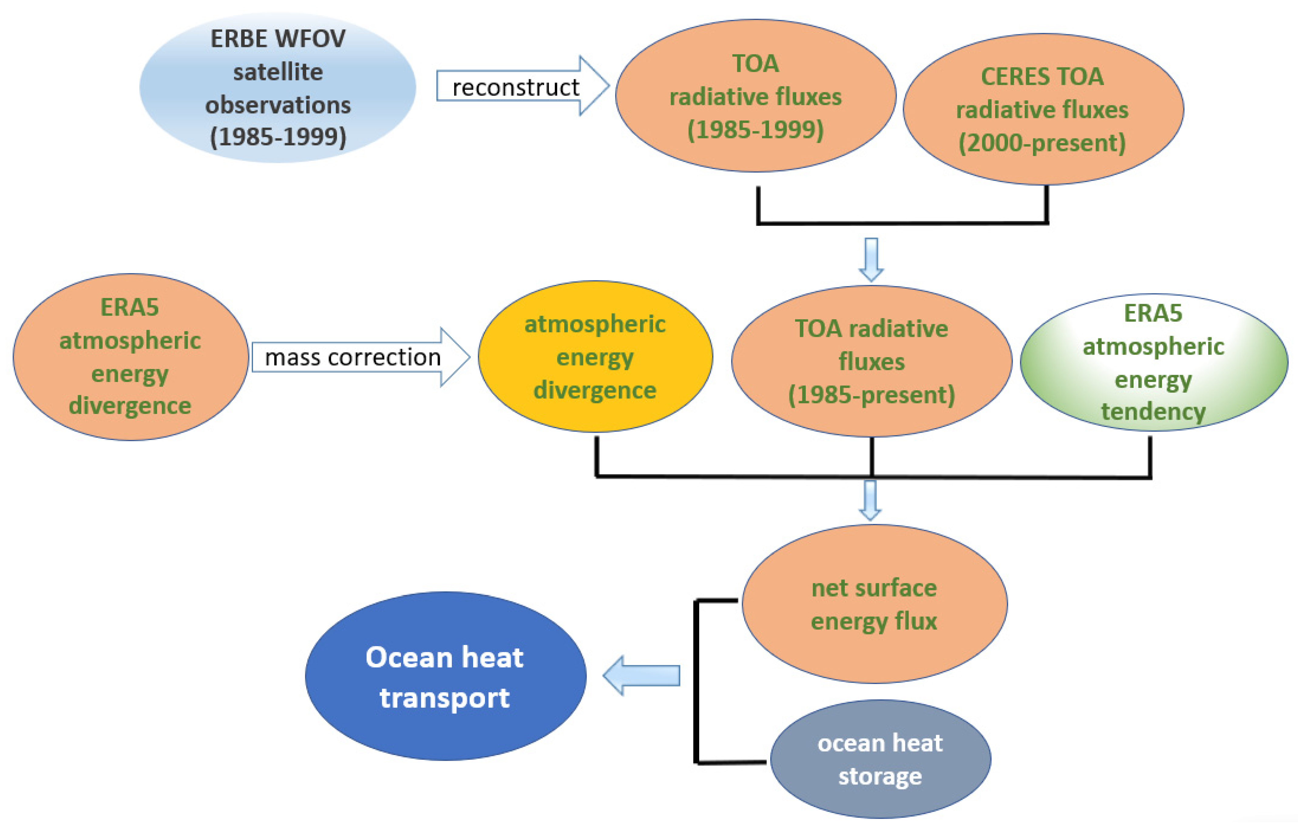
2. Data and Methods
3. Results
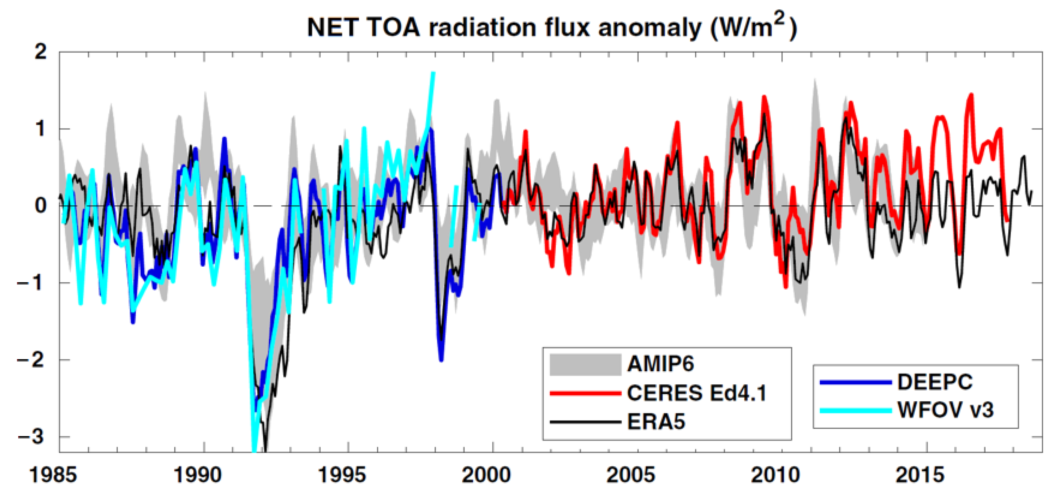
3.1. Net TOA Radiative Flux
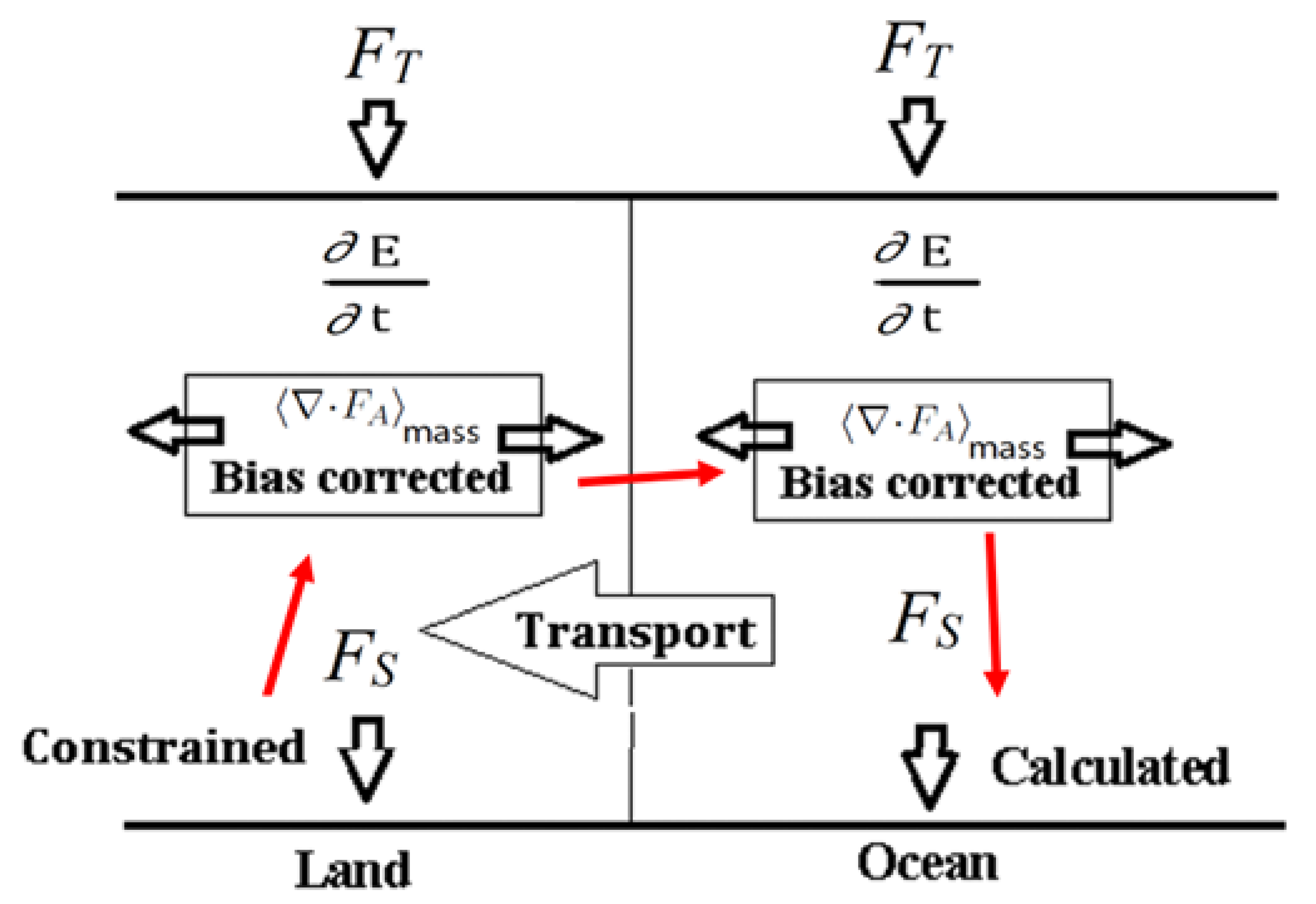
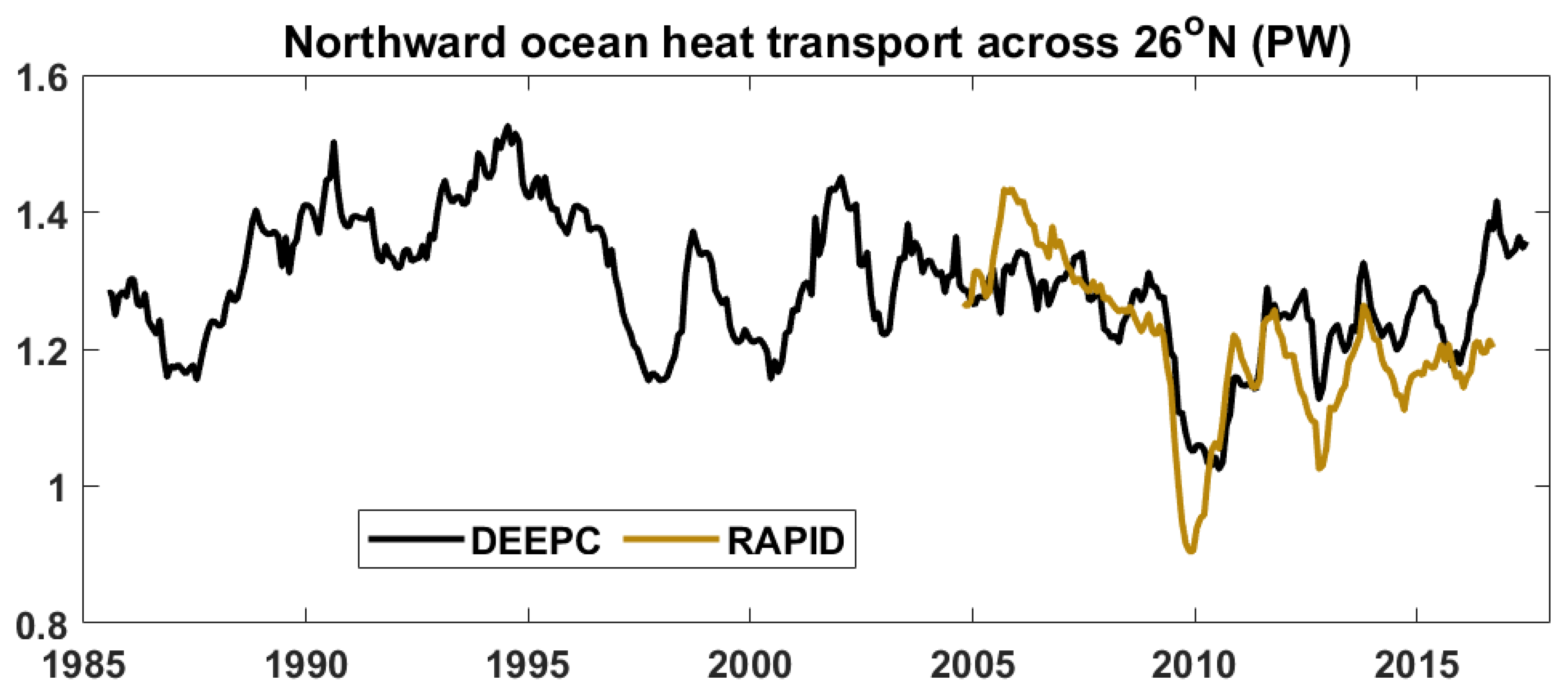
3.2. Energy Flow in the Earth System
4. Discussion
5. Conclusions
Author Contributions
Funding
Data Availability Statement
Acknowledgments
Conflicts of Interest
References
- Allan, R.P.; Liu, C.; Loeb, N.B.; Palmer, M.D.; Roberts, M.; Smith, D.; Vidale, P.-L. Changes in global net radiative imbalance 1985–2012. Geophys. Res. Lett. 2014, 41, 5588–5597. [Google Scholar] [CrossRef] [PubMed]
- Loeb, N.G.; Lyman, J.M.; Johnson, G.C.; Allan, R.; Doelling, D.R.; Wong, T.; Soden, B.; Stephens, G.L. Observed changes in top-of-atmosphere radiation and upper-ocean heating consistent within uncertainty. Nat. Geosci. 2012, 5, 110–113. [Google Scholar] [CrossRef]
- Wong, T.; Wielicki, B.A.; Lee, R.B.; Smith, G.L.; Bush, K.A.; Willis, J.K. Reexamination of the observed decadal variability of the earth radiation budget using altitude-corrected ERBE/ ERBS nonscanner WFOV data. J. Clim. 2006, 19, 4028–4040. [Google Scholar] [CrossRef]
- Dee, D.P.; Uppala, S.M.; Simmons, A.J.; Berrisford, P.; Poli, P.; Kobayashi, S.; Andrae, U.; Balmaseda, M.A.; Balsamo, G.; Bauer, P.; et al. The ERA-Interim reanalysis: Confguration and performance of the data assimilation system. Q. J. R. Meteorol. Soc. 2011, 137, 553–597. [Google Scholar] [CrossRef]
- Liu, C.; Allan, R.P.; Mayer, M.; Hyder, P.; Loeb, N.; Roberts, C.D.; Edwards, J.M.; Vidale, P.-L. Evaluation of satellite and reanalysisbased global net surface energy flux and uncertainty estimates. J. Geophys. Res. Atmos. 2017, 122, 6250–6272. [Google Scholar] [CrossRef] [Green Version]
- Hersbach, H.; Bell, B.; Berrisford, P.; Hirahara, S.; Horanyi, A.; Muñoz-Sabater, J.; Nicolas, J.; Peubey, C.; Radu, R.; Schepers, D.; et al. The ERA5 global reanalysis. Q. J. R. Meteorol. Soc. 2020, 146, 1999–2049. [Google Scholar] [CrossRef]
- Liu, C.; Allan, R.P.; Mayer, M.; Hyder, P.; Desbruyères, D.; Cheng, L.; Xu, J.; Xu, F.; Zhang, Y. Variability in the global energy budget and transports 1985−2017. Climate Dyn. 2020, 55, 3381–3396. [Google Scholar] [CrossRef]
- Trenberth, K.E.; Zhang, Y.; Fasullo, J.T.; Cheng, L. Observationbased estimates of global and basin ocean meridional heat transport time series. J. Clim. 2019, 32, 4567–4583. [Google Scholar] [CrossRef]
- Trenberth, K.E. Climate diagnostics from global analyses: Conservation of mass in ECMWF analyses. J. Clim. 1991, 4, 707–722. [Google Scholar] [CrossRef]
- Mayer, M.; Haimberger, L. Poleward atmospheric energy transports and their variability as evaluated from ECMWF reanalysis data. J. Clim. 2012, 25, 734–752. [Google Scholar] [CrossRef]
- Liu, C.; Allan, R.P.; Berrisford, P.; Mayer, M.; Hyder, P.; Loeb, N.; Smith, D.; Vidale, P.-L.; Edwards, J.M. Combining satellite observations and reanalysis energy transports to estimate global net surface energy fluxes 1985–2012. J. Geophys. Res. Atmos. 2015, 120, 9374–9389. [Google Scholar] [CrossRef] [Green Version]
- Mayer, M.; Haimberger, L.; Edwards, J.M.; Hyder, P. Toward consistent diagnostics of the coupled atmosphere and ocean energy budgets. J. Clim. 2017, 30, 9225–9246. [Google Scholar] [CrossRef]
- Mayer, J.; Mayer, M.; Haimberger, L. Consistency and homogeneity of atmospheric energy, moisture, and mass budgets in ERA5. J. Clim. 2021, 34, 3955–3974. [Google Scholar] [CrossRef]
- Trenberth, K.E.; Zhang, Y. Observed interhemispheric meridional heat transports and the role of the Indonesian throughfow in the Pacifc Ocean. J. Clim. 2019, 32, 8523–8536. [Google Scholar] [CrossRef]
- Trenberth, K.E.; Solomon, A. The global heat balance: Heat transports in the atmosphere and ocean. Clim. Dyn. 1994, 10, 107–134. [Google Scholar] [CrossRef]
- Arias, P.; Bellouin, N.; Coppola, E.; Jones, R.; Krinner, G.; Marotzke, J.; Zickfeld, K. Technical Summary. In Climate Change 2021: The Physical Science Basis. Contribution of Working Group I to the Sixth Assessment Report of the Intergovernmental Panel on Climate Change; Masson-Delmotte, V., Ed.; Cambridge University Press: Cambridge, UK, 2021; in press. [Google Scholar]
- Smeed, D.; McCarthy, G.; Rayner, D.; Moat, B.I.; Johns, W.E.; Baringer, M.O.; Meinen, C.S. Atlantic Meridional Overturning Circulation Observed by the RAPID-MOCHA-WBTS (RAPID-Meridional Overturning Circulation and Heatfux Array-Western Boundary Time Series) Array at 26N from 2004 to 2017; British Oceanographic Data Centre, Natural Environment Research Council. 2017. Available online: https://rmets.onlinelibrary.wiley.com/doi/abs/10.1002/qj.828 (accessed on 10 November 2019).
- Zuo, H.; Balmaseda, M.A.; Tietsche, S.; Mogensen, K.; Mayer, M. The ECMWF operational ensemble reanalysis–analysis system for ocean and sea ice: A description of the system and assessment. Ocean Sci. 2019, 15, 779–808. [Google Scholar] [CrossRef] [Green Version]
- Liu, C.; Yang, Y.; Liao, X.; Cao, N.; Liu, J.; Ou, N.; Allan, R.P.; Jin, L.; Chen, N.; Zheng, R. Discrepancies in simulated ocean net surface heat fluxes over the North Atlantic. Adv. Atmos. Sci. 2022, 39, 1941–1955. [Google Scholar] [CrossRef]
- Chiodo, G.; Haimberger, L. Interannual changes in mass consistent energy budgets from ERA-Interim and satellite data. J. Geophys. Res. 2010, 115, D02112. [Google Scholar] [CrossRef]
- Simmons, A.J.; Burridge, D.M. An energy and angular-momentum conserving vertical finite-difference scheme and hybrid vertical coordinates. Mon. Weather Rev. 1981, 109, 758–766. [Google Scholar] [CrossRef]
- Loeb, N.G.; Wang, H.L.; Cheng, A.N.; Kato, S.; Fasullo, J.T.; Xu, K.-M.; Allan, R.P. Observational constraints on atmospheric and oceanic cross-equatorial heat transports: Revisiting the precipitation asymmetry problem in climate models. Clim. Dyn. 2016, 46, 3239–3257. [Google Scholar] [CrossRef]
- Trenberth, K.E.; Fasullo, J.T. Atlantic meridional heat transports computed from balancing Earth’s energy locally. Geophys. Res. Lett. 2017, 44, 1919–1927. [Google Scholar] [CrossRef]
- Loeb, N.G.; Doelling, D.R.; Wang, H.; Su, W.; Nguyen, C.; Corbett, J.G.; Liang, L.; Mitrescu, C.; Rose, F.G.; Kato, S. Clouds and the earth’s radiant energy system (CERES) energy balanced and flled (EBAF) top-of-atmosphere (TOA) edition 4.0 data product. J. Clim. 2018, 31, 895–918. [Google Scholar] [CrossRef]
- Wu, T.; Yu, R.; Lu, Y.; Jie, W.; Fang, Y.; Zhang, J.; Zhang, L.; Xin, X.; Li, L.; Wang, Z.; et al. BCC-CSM2-HR: A high-resolution version of the Beijing Climate Center Climate System Model. Geosci. Model Dev. 2021, 14, 2977–3006. [Google Scholar] [CrossRef]
- Danabasoglu, G.; Lamarque, J.-F.; Bacmeister, J.; Bailey, D.A.; DuVivier, A.K.; Edwards, J.; Emmons, L.K.; Fasullo, J.; Garcia, R.; Gettelman, A.; et al. The Community Earth System Model Version 2 (CESM2). J. Adv. Model. Earth Syst. 2020, 12, e2019MS001916. [Google Scholar] [CrossRef] [Green Version]
- Eyring, V.; Bony, S.; Meehl, G.A.; Senior, C.A.; Stevens, B.; Stouffer, R.J.; Taylor, K.E. Overview of the Coupled Model Intercomparison Project Phase 6 (CMIP6) experimental design and organization. Geosci. Model Dev. 2016, 9, 1937–1958. [Google Scholar] [CrossRef] [Green Version]
- Davini, P.; von Hardenberg, J.; Corti, S.; Christensen, H.M.; Juricke, S.; Subramanian, A.; Watson, P.A.G.; Weisheimer, A.; Palmer, T.N. Climate SPHINX: Evaluating the impact of resolution and stochastic physics parameterisations in the EC-Earth global climate model. Geosci. Model Dev. 2017, 10, 1383–1402. [Google Scholar] [CrossRef] [Green Version]
- He, B.; Liu, Y.; Wu, G.; Bao, Q.; Zhou, T.; Wu, X.; Wang, L.; Li, J.; Wang, X.; Li, J.; et al. CAS FGOALS-f3-L model datasets for CMIP6 GMMIP Tier-1 and Tier-3 experiments. Adv. Atmos. Sci. 2020, 37, 18–28. [Google Scholar] [CrossRef] [Green Version]
- Williams, K.D.; Harris, C.M.; Bodassalcedo, A.; Camp, J.; Comer, R.E.; Copsey, D.; Fereday, D.; Graham, T.; Hill, R.; Hinton, T.; et al. The Met Ofce Global Coupled model 2.0 (GC2) confguration. Geosci. Model Dev. 2015, 88, 1509–1524. [Google Scholar] [CrossRef] [Green Version]
- Boucher, O.; Denvil, S.; Levavasseur, G.; Cozic, A.; Caubel, A.; Foujols, M.-A.; Meurdesoif, Y.; Ghattas, J. IPSL IPSL-CM6A-LR model output prepared for CMIP6 HighResMIP. Earth Syst. Grid Fed. 2019. [Google Scholar] [CrossRef]
- Tatebe, H.; Ogura, T.; Nitta, T.; Komuro, Y.; Ogochi, K.; Takemura, T.; Sudo, K.; Sekiguchi, M.; Abe, M.; Saito, F.; et al. Description and basic evaluation of simulated mean state, internal variability, and climate sensitivity in MIROC6. Geosci. Model Dev. 2019, 12, 2727–2765. [Google Scholar] [CrossRef]
- Yukimoto, S.; Kawai, H.; Koshiro, T.; Oshima, N. The Meteorological Research Institute Earth System Model version 2.0, MRI-ESM2.0: Description and basic evaluation of the physical component. J. Meteor. Soc. Jpn. 2019, 97, 931–965. [Google Scholar] [CrossRef] [Green Version]
- Park, S.; Shin, J.; Kim, S.; Oh, E. Global Climate Simulated by the Seoul National University Atmosphere Model Version 0 with a Unified Convection Scheme (SAM0-UNICON). J. Clim. 2019, 32, 2917–2949. [Google Scholar] [CrossRef]
- Cheng, L.J.; Trenberth, K.E.; Fasullo, J.; Boyer, T.; Abraham, J.; Zhu, J. Improved estimates of ocean heat content from 1960 to 2015. Sci. Adv. 2017, 3, e1601545. [Google Scholar] [CrossRef] [PubMed] [Green Version]
- Gentine, P.; Seneviratne, S.I.; Beltrami, H.; Davin, E.; Meier, R.; García-García, A.; Cuesta-Valero, F.J. Large recent continental heat storage. In AGU Fall Meeting Abstracts; American Meteorological Society: San Francisco, CA, USA, 2019; Volume 2019, p. GC51J-1078. [Google Scholar]
- Terai, C.R.; Caldwell, P.M.; Klein, S.A.; Tang, Q.; Branstetter, M.L. The atmospheric hydrologic cycle in the ACME v0.3 model. Clim. Dyn. 2018, 50, 3251–3279. [Google Scholar] [CrossRef]
- Qu, J.; Truhan, J.J.; Dai, S.; Luo, H.; Blau, P.J. An assessment of air-sea heat fuxes from ocean and coupled reanalyses. Clim. Dyn. 2015, 22, 207–214. [Google Scholar] [CrossRef] [Green Version]
- Roberts, M.J.; Hewitt, H.T.; Hyder, P.; Ferreira, D.; Josey, S.A.; Mizielinski, M.; Shelly, A. Impact of ocean resolution on coupled airsea fuxes and large-scale climate. Geophys. Res. Lett. 2016, 43, 10430–10438. [Google Scholar] [CrossRef] [Green Version]
- Roberts, C.D.; Palmer, M.D.; Allan, R.P.; Desbruyeres, D.G.; Hyder, P.; Liu, C.; Smith, D. Surface fux and ocean heat transport convergence contributions to seasonal and interannual variations of ocean heat content. J Geophys. Res Ocean. 2017, 122, 726–744. [Google Scholar] [CrossRef]
- Senior, C.A.; Andrews, T.; Burton, C.; Chadwick, R.; Copsey, D.; Graham, T.; Hyder, P.; Jackson, L.; McDonald, R.; Ridley, J.; et al. Idealised climate change simulations with a high resolution physical model: HadGEM3-GC2. J. Adv. Model Earth Syst. 2016, 8, 813–830. [Google Scholar] [CrossRef]
- Hyder, P.; Edwards, J.M.; Allan, R.P.; Hewitt, H.T.; Bracegirdle, T.J.; Gregory, J.M.; Belcher, S.E. Critical Southern Ocean climate model biases traced to atmospheric model cloud errors. Nat. Commun. 2018, 9, 3625. [Google Scholar] [CrossRef] [Green Version]
- Mignac, D.; Ferreira, D.; Haines, K. South Atlantic meridional transports from NEMO-based model simulations and reanalyses. Ocean Sci. 2018, 14, 53–68. [Google Scholar] [CrossRef]
- Cheng, L.; Trenberth, K.E.; Fasullo, J.; Mayer, M.; Balmaseda, M.; Zhu, J. Evolution of ocean heat content related to ENSO. J. Clim. 2019, 32, 3529–3556. [Google Scholar] [CrossRef]
- Allison, L.C.; Palmer, M.D.; Allan, R.P.; Hermanson, L.; Liu, C.L.; Smith, D.M. Observations of planetary heating since the 1980s from multiple independent datasets. Environ. Res. Commun. 2020, 2, 101001. [Google Scholar] [CrossRef]
- Bryden, H.L.; Johns, W.E.; King, B.A.; McCarthy, G.; Mcdonagh, E.L.; Moat, B.I.; Smeed, D.A. Reduction in ocean heat transport at 26° N since 2008 cools the eastern subpolar gyre of the North Atlantic Ocean. J. Clim. 2020, 33, 1677–1689. [Google Scholar] [CrossRef]
- Mayer, J.; Mayer, M.; Haimberger, L.; Liu, C. Comparison of surface energy fluxes from global to local scale. J. Clim. 2022, 35, 4551–4569. [Google Scholar] [CrossRef]
- Andrews, T.; Bodas-Salcedo, A.; Gregory, J.M.; Dong, Y.; Armour, K.C.; Paynter, D.; Lin, P.; Modak, A.; Mauritsen, T.; Cole, J.N.S.; et al. On the effect of historical SST patterns on radiative feedback. J. Geophys. Res. 2022, 87, 161–177. [Google Scholar] [CrossRef]
- Kato, S.; Loeb, N.G.; Fasullo, J.T.; Trenberth, K.E.; Lauritzen, P.H.; Rose, F.G.; Rutan, D.A.; Satoh, M. Regional Energy and Water Budget of a Precipitating Atmosphere over Ocean. J. Clim. 2021, 34, 4189–4205. [Google Scholar] [CrossRef]
- Trenberth, K.E.; Fasullo, J.T. Applications of an updated atmospheric energetics formulation. J. Clim. 2018, 31, 6263–6279. [Google Scholar] [CrossRef]


| Data Set | Period (in This Study) | Horizontal Resolution | References |
|---|---|---|---|
| DEEPC v5.0 | 1985–2017 | 0.7° × 0.7° | Liu et al. (2020) [7] |
| WFOV v3.0 | 1985–1999 | 10° × 10° | Wong et al. (2006) [3] |
| CERES Ed4.1 | 2001–2019 | 1.0° × 1.0° | Loeb et al. (2018) [24] |
| RAPID | 2004–2017 | Smeed et al. (2017) [17] | |
| ERA5 | 1985–2018 | 0.25° × 0.25° | Hersbach et al. 2020 [6] |
| ORAS5 | 1993–2016 | 1.0° × 1.0° | Zuo et al. (2019) [18] |
| AMIP6 simulations: | |||
| BCC-CSM2-MR | 1985–2014 | 1.125° × 1.125° | Wu et al. (2021) [25] |
| CESM2 | 0.94° × 1.25° | Danabasoglu et al. (2020) [26] | |
| CNRM-CM6-1 | 1.40° × 1.40° | Eyring et al. (2016) [27] | |
| EC-Earth3-Veg | 0.70° × 0.70° | Davini et al. (2017) [28] | |
| FGOALS-f3-L | 1.0° × 1.25° | He et al. (2020) [29] | |
| HadGEM3-GC31-LL | 1.25° × 1.875° | Williams et al. (2015) [30] | |
| IPSL-CM6A-LR | 1.25° × 1.25° | Boucher et al. (2019) [31] | |
| MIROC6 | 1.43° × 1.43° | Tatebe et al. (2019) [32] | |
| MRI-ESM2-0 | 1.125° × 1.125° | Yukimoto et al. (2019) [33] | |
| SAM0-UNICON | 0.94° × 1.25° | Park et al. (2019) [34] |
Publisher’s Note: MDPI stays neutral with regard to jurisdictional claims in published maps and institutional affiliations. |
© 2022 by the authors. Licensee MDPI, Basel, Switzerland. This article is an open access article distributed under the terms and conditions of the Creative Commons Attribution (CC BY) license (https://creativecommons.org/licenses/by/4.0/).
Share and Cite
Liu, C.; Chen, N.; Long, J.; Cao, N.; Liao, X.; Yang, Y.; Ou, N.; Jin, L.; Zheng, R.; Yang, K.; et al. Review of the Observed Energy Flow in the Earth System. Atmosphere 2022, 13, 1738. https://doi.org/10.3390/atmos13101738
Liu C, Chen N, Long J, Cao N, Liao X, Yang Y, Ou N, Jin L, Zheng R, Yang K, et al. Review of the Observed Energy Flow in the Earth System. Atmosphere. 2022; 13(10):1738. https://doi.org/10.3390/atmos13101738
Chicago/Turabian StyleLiu, Chunlei, Ni Chen, Jingchao Long, Ning Cao, Xiaoqing Liao, Yazhu Yang, Niansen Ou, Liang Jin, Rong Zheng, Ke Yang, and et al. 2022. "Review of the Observed Energy Flow in the Earth System" Atmosphere 13, no. 10: 1738. https://doi.org/10.3390/atmos13101738