Article

Application of Empirical Orthogonal Function Analysis to 1 km Ensemble Simulations and Himawari–8 Observation in the Intensification Phase of Typhoon Hagibis (2019)

Meteorological Research Institute, Japan Meteorological Agency, 1–1 Nagamine, Tsukuba 305-0052, Ibaraki, Japan
*
Author to whom correspondence should be addressed.
Atmosphere 2022, 13(10), 1559; https://doi.org/10.3390/atmos13101559
Submission received: 23 August 2022 / Revised: 14 September 2022 / Accepted: 20 September 2022 / Published: 23 September 2022
(This article belongs to the Special Issue Feature Papers in Meteorological Science)

Abstract

:
An empirical orthogonal function (EOF) analysis was performed for the inner core of Typhoon Hagibis (2019) in the intensification phase. The Himawari–8 geostationary infrared (IR) brightness temperature (BT) collocated at the Hagibis’s center was combined with the IR BT simulated by a radiative transfer model, with 1 km ensemble simulations conducted by an atmosphere model and the coupled atmosphere–wave–ocean model. The ensemble simulations were conducted under one control atmospheric initial condition and the 26 perturbed ones with two different oceanic initial conditions. The first four EOF modes showed symmetric and asymmetric patterns such as a curved band, cloud dense overcast, and eye pattern used in the classification of the Dvorak technique. The influence of ocean coupling on the modes appeared only in the early intensification phase but was relatively small compared to the difference from the Himawari–8 observations. While ocean coupling and different oceanic initial condition quantitatively affected the IR BT, the normalized amplitude for the first EOF mode did not become close to that of the Himawari–8 observation in the late intensification phase. The intensification rate in the late intensification phase was inconsistent between the simulation results and the estimate from the Himawari–8 normalized amplitude by multiple linear regression analysis.

1. Introduction

Principal component analysis (PC) (or empirical orthogonal function analysis (EOF)) is a method that can select representative modes by linear mode expansion so as to explain the largest variance, which is obtained by solving for the eigenvalues and eigenvectors of the variance–covariance matrix. Although the representative modes are not necessarily connected with physical processes, previous studies have indicated that the modes are sometimes associated with internal variability in the atmosphere and ocean, and some indices have been used in climate change monitoring, such as Arctic oscillation [1], boreal summer intraseasonal oscillation [2], and Madden–Jullian oscillation [3]. PC has also been recently applied to study winter storms on the US east coast [4,5]. As an example of tropical cyclone (TC) studies, the EOF analysis for TC heat potential suggested that ocean warming may be responsible for lowering of the central pressure of Typhoon Hagibis in 2019 [6]. This result was supported by the results of ensemble experiments with a perturbed atmospheric initial condition by comparing the differences in simulated central pressures between the experiments with an oceanic daily initial condition and the climatological mean [7].
Ensemble experiments have become a mainstream method in stochastic forecasting and projecting of weather and climate with the improvement of computer technology. TC forecasting is no exception, with a multicenter ensemble of deterministic forecasts collected from major numerical prediction centers and an ensemble product that is calculated by a single model with different initial conditions created by adding perturbations [8]. The application of the ensemble method to typhoon forecasting has contributed to a steady improvement in TC track forecasting [9]. However, TC intensity forecasting has improved more slowly than TC track forecasting [10]. Although technologies associated with observations, TC analysis and TC forecasting, are becoming more sophisticated [11], understanding a real TC intensity remains a scientific challenge.
Since aircraft observations have not been conducted operationally in the Northwest Pacific since 1987, the method proposed by Dvorak [12] has been one of the important methods for estimating TC intensity for meteorological centers in the world. There have been many studies on the development of objective Dvorak methods [13,14] and TC intensity analysis using various satellite data [15]. Due to the accuracy of the retrieved physical quantity and frequency of observation, such analysis data are usually used as complementary information to the TC intensity estimate based on the Dvorak analysis. However, various problems have been pointed out, such as problems in TC intensity in mid–latitudes where water temperatures become low [14]. With limited opportunities to verify Dvorak–based TC intensities from aircraft or the other in situ observations, there is also a question of whether the relationship between TC intensities and cloud systems, such as band, cloud dense overcast, and eye patterns will remain unchanged under increasing water temperatures and global warming [6,16].
Numerical simulations by a sophisticated numerical model with a high resolution are an effective way for accurately estimating TC intensity in that the cloud systems represented by simulated brightness temperatures (BTs), which are dynamically and thermodynamically linked to simulated central pressures and maximum wind speeds. However, there is still room for further study on how to efficiently analyze the enormous data obtained from a large ensemble simulation. Therefore, we attempt to interpret the relation of Dvorak BT patterns to representative PC or EOF modes within the framework of TC inner–core dynamics and thermodynamics and multiple linear regression analysis. To conduct EOF analysis, we combined the Himawari–8 BT [17] with the results of ensemble simulations, conducted with/without ocean coupling, under two different oceanic initial conditions. In this study, we conducted an EOF analysis for a limited area collocated at the TC center and the phase was focused on the intensification of Hagibis. Hagibis was selected in this study because it caused river flooding over a broad area in Japan and was of great social concern [6] and preliminarily ensemble simulations have been already conducted [7]. However, the intensification and the maximum intensity of Hagibis was not well simulated in the ensemble experiment. In addition, the results of ensemble simulations have not been validated with the Himawari–8 BT. One of the objectives of this study is to understand to what extent the results of ensemble simulations could reproduce the ‘real’ cloud patterns in the intensification phase of Hagibis observed by Himawari–8. This objective includes the question of whether differences in the oceanic preexisting condition and ocean coupling do influence the relationship between TC intensities and cloud systems. The clarification is expected to contribute to the improvement of TC intensity analysis in the intensification phase, although this study is only a case study.
Previous studies have indicated that TC intensification is affected by deep–layer vertical wind shear (VWS) [18,19], although the VWS is not a dominant factor of the onset of rapid intensification (RI) [20,21]. There have been a number of studies on the relation between deep–layer VWS and RI and structural changes [21,22,23,24,25,26,27]. The majority of RI cases occurred in low VWS (<4.5 m s−1) [22]. The moderate VWS (4.5–11 m s−1) resulted in the increase in upshear outflow, which was associated with active convection on the upshear side [23,24], resulting in RI. VWS is sometimes divided into environmental VWS and TC–induced VWS. The magnitude of environmental VWS affected the size and strength of the warm core at around the TC center in addition to TC intensification rate and structural change [26]. Even under strong environmental wind shear (>10 m s−1), the TC–induced outflow withstood the strong upper–tropospheric environmental flow [27]. The intensified TC–induced outflow blocked the upper–level environmental flow, which led to a decrease in the TC–induced VWS [23]. The magnitude of environmental VWS also affected the TC inner–core structure, such as monopole, ring–like, and wavenumber–1 asymmetric patterns (Figure 3 in [22]). A study using the results of an ensemble simulation indicated that TC intensification rates differed between ring–like and monopole states [28]. A question arises as to whether the inner–core structural changes and associated intensity changes, particularly simulated TC intensification rates, are connected with those indicated by the Dvorak analysis. Thus, the other objective of this study is to determine the extent to which the dynamic and thermodynamic processes obtained from numerical simulations explain a real TC intensification and its structural change. The thermodynamic processes include the effects of ocean coupling and the oceanic preexisting condition. The clarification is expected to contribute to the improvement of numerical models and TC forecasting.
The remainder of this paper is organized as follows: Section 2 briefly describes the Himawari–8 data, numerical models, their configuration, and specification for a series of ensemble numerical simulations, and how to apply an EOF analysis to them. Section 3 shows the results of ensemble simulations and those of EOF analysis in the entire, early, and late intensification phases, respectively. Section 3 also shows the results of a multiple linear regression analysis using a 6 h simulated central pressure tendency and the Himawari–8 normalized amplitude of the first four EOF modes. Section 4 discusses the availability and limit of the application of a EOF analysis to TC ensemble simulations. Section 5 summarizes this study.

2. Data and Methods

This study used full–disk data of infrared (IR) satellite BT (the unit is K) of Himawari–8 band 13 (b13: the wavelength is 10.4 μm) [17] every 3 h from 6 to 7 October in 2019. The reference of Hagibis was obtained from the Regional Specialized Meteorological Center (RSMC) Tokyo best–track archive [29] and Joint Typhoon Warning Center best–track archive [30]. The ensemble simulations were conducted by a nonhydrostatic atmosphere model (NHM) and the atmosphere–wave–ocean coupled model (CPL) [31] with oceanic daily initial condition and the climatological mean oceanic condition, the average for 26 years from 1993 to 2018 (AVE). The specifications are listed in Table 1. NHM, CPL, NHMAVE, and CPLAVE are experiment names that will be used thereafter.
In Table 1, we used an explicit three–ice bulk microphysics scheme [32,33]. Air–sea momentum fluxes and sensible and latent heat fluxes, with exchange coefficients for air–sea momentum and enthalpy transfers over the sea, were based either on bulk formulas of Kondo [34] or, when the ocean wave model was coupled, on the roughness lengths proposed by Taylor and Yelland [35], a sea spray formulation [31], a turbulent closure model [36,37], and a radiation scheme [38]. No cumulus parameterization was used in the ensemble simulations
The model configuration for ensemble experiments is shown in Table 2. The initial time was 00 UTC on 6 October in 2019. The CPL consists of the nonhydrostatic atmosphere model (same as NHM), ocean wave model, and ocean model [31]. The time step of each component was different as was shown in Table 2. The horizontal resolution of NHM and CPL was 1 km. The computational domain was single and covered the domain of 1620 km (west to east) × 990 km (south to north), centered at 15° N, 150° E in the Lamber Conformal Conic projection. The NHM used 55 levels in vertical coordinates, with the intervals ranging from 40 m for the near–surface layer to 1013 m for the uppermost layer, and the top height was approximately 27 km. Sea surface temperature (SST) at the initial time was created by linear interpolation from analyzed data obtained from the microwave optimally interpolated SST daily product (obtained from the Remote Sensing Systems site [39]). Climatological mean SST on 5 October was calculated as the average for 20 years during 1999–2018 from the SST daily product. In order to create the oceanic initial condition, except for SST, we used the North Pacific version of Four–dimensional variational Ocean ReAnalysis dataset for the western North Pacific (FORA) spanning 1996–2015 [40] and the subsequent oceanic analysis data operationally analyzed in the Japan Meteorological Agency (JMA) from January 2016. The horizontal resolution was 0.5° in the longitude–latitude coordinate system. Climatological mean ocean initial condition on 5 October was calculated by linear interpolation as the average for 26 years during 1993–2018 by using FORA dataset (from 1993 to 2015) and JMA dataset (2016–2018).
The atmospheric initial and boundary conditions in the control run were created by linear interpolation from JMA 6 hourly global atmospheric analysis data with a horizontal grid spacing of approximately 20 km. The interval of the atmospheric boundary condition was 6 h. In addition, global atmospheric ensemble prediction data with a horizontal grid spacing of 1.25° obtained from JMA, of which the number of ensemble members was 26, were used to add perturbations to the atmospheric initial condition in the control run. VWS was calculated from the objective global analysis as the difference in horizontal wind speeds between 850 hPa and 200 hPa levels in the annulus between 100 km and 800 km from the TC center. For simulation results, VWS was calculated as the difference in horizontal wind speeds between the 13th (~1500 m) and 38th (~14,000 m) levels in the annulus, between 100 and 500 km from the TC center. The radiative transfer for television infrared observation satellite operational vertical sounder TOVS (RTTOV) [41] was used for simulating the IR BT of b13 collocated at the TC center in each ensemble simulation. An EOF analysis was performed by changing a Fortran code used by Wada and Chan [11] and by combining the Himawari–8 geostationary IR BT of b13 collocated at the TC center with the simulated IR BT in the NHM, CPL, NHMAVE, and CPLAVE experiments (Figure 1).

3. Results

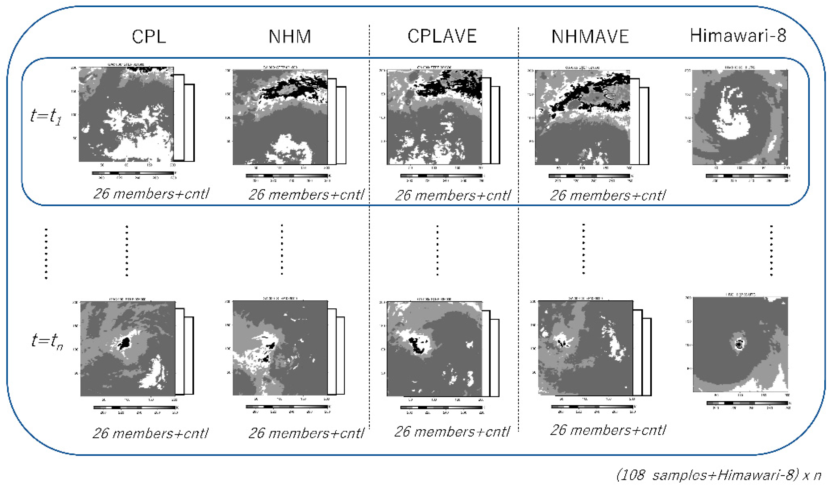
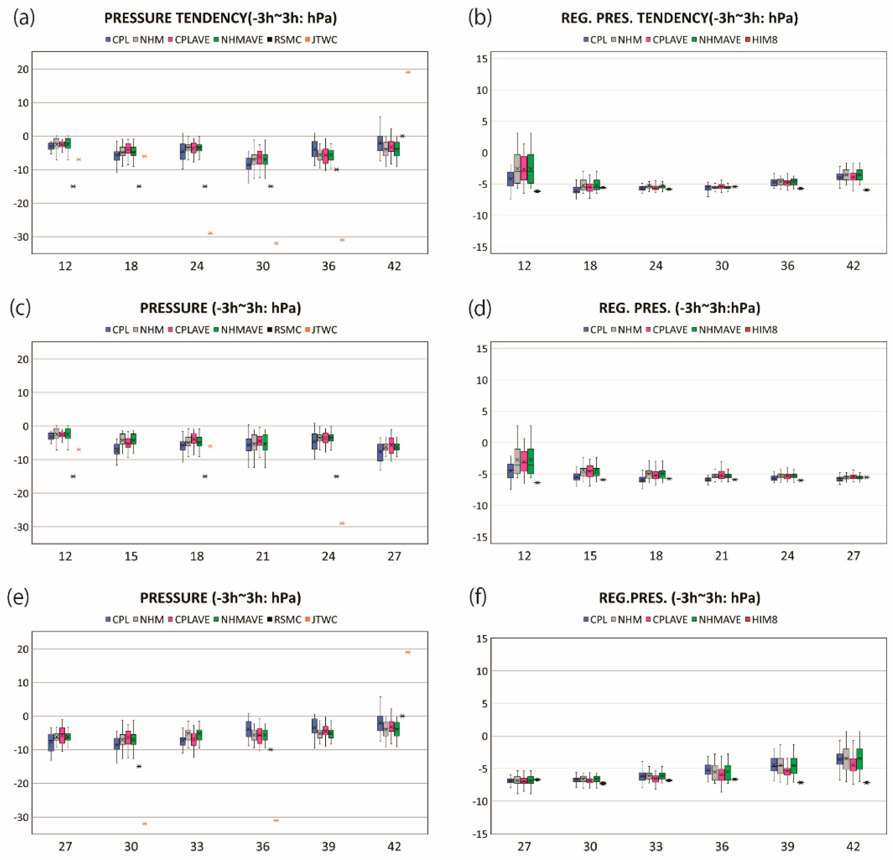
3.1. Results of Ensemble Simulations

Hagibis rapidly enlarged its size from its genesis at 18 UTC on October 5 in 2019 (15.1° N, 157.4° E) to its RI. RI is usually defined as the 95th percentile of all 24 h over–water intensity changes, corresponding to approximately +15 m s−1 or greater [19]. From 00 UTC on 6 October to 00UTC on 8 October, while Hagibis moved west–northwestward, it rapidly intensified and reached the minimum central pressures of 915 hPa (RSMC–Tokyo: Black line in Figure 2a) and 890 hPa (JTWC: Red line in Figure 2a). The west–northwestward movement of Hagibis was reasonably simulated in all ensemble experiments (Figure 2a). In Figure 2a, however, the tracking appears to start from 6 h because the center location of simulated TC from 0 h to 6 h integration time was detected near the TC position at 6 h. The tracking method used in this study was simple: The location of minimum sea–level pressure near the RSMC–Tokyo best–track position was detected at 0 h and then the location at the next output integration time was tracked within an area of 2° × 2° degrees, centered at the previous TC position. Therefore, the period from 0 h to 12 h integration time was not used for the EOF analysis in this study. In addition, the simulated TC was close to the north and western edges of the computational domain after 42 h. This is why the analysis period ranged from 12 h to 42 h integration times.
Figure 2b shows the timeseries of RSMC–Tokyo best–track, JTWC best–track, and simulated central pressures in the NHM, CPL, NHMAVE, and CPLAVE ensemble experiments. It should be mentioned that this study focuses only on the central pressure as an indicator of TC intensity. The timeseries of simulated central pressures is depicted as a box–and–whisker plot for each ensemble experiment. Each box in Figure 2b shows an interquartile range of normalized amplitude from the 25th percentile to 75th percentile, with the lowest and highest data points in each ensemble simulation excluding any outliers. ‘X’ indicates the mean value and ‘−’ indicates the median.
All mean simulated central pressures reached their lowest value within 42 h (Figure 2b). The difference in mean simulated central pressures between the NHM, CPL, NHMAVE, and CPLAVE ensemble experiments was approximately 10 hPa at 42 h. The mean simulated central pressure in the NHM and CPL experiments with the oceanic initial condition created from the daily analysis was a lower mean than that in the CPLAVE and NHMAVE with the climatological mean oceanic initial condition. The mean simulated central pressure in the CPL (CPLAVE) experiment was higher than that in the NHM (NHMAVE) experiment due to the lowering of the simulated SST along the track during the integration [7]. These results were consistent with [31]. It should be noted that the RSMC–Tokyo and JTWC best–track archives showed a large difference in Hagibis’s central pressure, especially at 18 h (18 UTC on 6 October) and 36 h (12 UTC on 7 October). Due to the lack of in situ observations on the central pressure, it is not possible to conclude which is more accurate. Since the two best–track central pressures were based on TC intensity estimates based on the Himawari–8 IR BT data and the Dvorak method [12], it is possible to determine which is more accurate by comparing the simulated and observed IR BTs of b13 by considering the relation of simulated IR BT of b13 to the central pressure of simulated TC through the EOF analysis conducted in this study.
The simulated IR BT of b13 was calculated by RTTOV with the ensemble simulation results. A 200 × 200 grid area with the horizontal resolution of 1 km collocated at the TC center was extracted from each simulation result every 3 h from 12 h to 42 h integration times. Although the area includes the maximum wind speed radius of simulated Hagibis (40~50 km average), it does not necessarily include all the outer band area. Expanding the calculation area possibly reduced the ratio of the variation in the representative modes to the overall variation. Therefore, this study will mainly focus on the representative EOF modes of cloud dense occlusion (CDO) and eye (EYE) types based on the Dvorak method for simulated TC intensity.
Figure 3 shows the distribution of Himawari–8 IR BT of b13 around the TC center (Figure 3a–c) and that simulated by RTTOV with the simulation result conducted as the control run in the CPL experiment (Figure 3d–f) along with the VWS calculated with the global analysis data (Figure 3a–c) and the simulation result (Figure 3d–f) at the corresponding integration time, respectively. The vector of TC motion in Figure 3a–c was calculated by using the JMA early Dvorak positions 3 h before and after the specified time, while that in Figure 3d–f was calculated by using the simulated positions 3 h before and after the specified time in the CPL control experiment. The JMA early Dvorak dataset is a preliminary analysis for operational use before the best track is confirmed [42]. Although it is not definitive and subjective, it contains various information obtained from the Dvorak analysis. According to the JMA early Dvorak analysis, the cloud pattern showed a curved band at 18 UTC on 6 October, a CDO at 00 UTC on 7 October, and an EYE pattern at 06 UTC on 7 October, while the cloud pattern changed from poorly defined circulation to well defined circulation and then to EYE type according to the JTWC ATCF dataset [43].
A previous study [44] classified TCs in the Northwestern Pacific from 1998 to 2008 into 10 clusters by performing a PC analysis for the TCs that were collocated in a box area of 3° × 3° with the Tropical Rainfall Measuring’ Mission’s (TRMM) Microwave Imager (TMI) BT data. When focusing on the distribution within ~2° × 2° (200 km × 200 km), as addressed in Figure 3 with reference to 85 GHz PC results of [44], the results of the EOF analysis showed various patterns, such as monopole, ring–like, and wavenumber one patterns, which did not necessarily correspond one–to–one with the patterns in the Dvorak analysis [12]. The direction of VWS was southwestward in both the objective global analysis and simulation results, albeit with the differences in magnitude. The magnitude ranged approximately 5~8 m s−1, corresponding to the moderate VWS [21,23]. The direction of TC motion in Figure 3a–c was west–northwestward to westward, which was consistent with the direction in Figure 3d–f.
Figure 4 shows the horizontal distribution of the difference in IR BT of b13 between the Himawari–8 and the simulation by RTTOV in the CPL, CPLAVE, NHM, and NHMAVE control experiments at 06 UTC on 7 October. All experiments revealed that the distribution had a wavenumber–1 asymmetric pattern. The differences between Figure 4a,b and those between Figure 4c,d showed the effects of ocean coupling on the value of IR BT of b13. The ocean coupling led to the slight difference in the wavenumber–1 asymmetric pattern of IR BT of b13. The similar difference was caused by the difference in the oceanic initial condition. However, both differences on the asymmetric pattern could not explain the differences in the simulated central pressures shown in Figure 2b, although the curved–band pattern shown in Figure 4 may be affected by the difference in simulated tangential winds (not shown). The result implied that oceanic influences appeared in the simulated central pressure values but were less apparent in the cloud patterns in the upper troposphere at around the TC center.
The EOF analysis was performed for the following three intensification periods by combining the IR BT of b13 by RTTOV with ensemble simulations with the Himawari–8 IR BT of b13. Each calculation was performed 100 times to apply a bootstrap method, allowing for the duplication of ensemble members and substituting combinations.
  • 12−42 h every 6 h: the entire intensification phase.
  • 12−27 h every 3 h: the early intensification phase from poorly defined circulation to well defined circulation.
  • 27−42 h every 3 h: the late intensification phase from well–defined circulation to EYE.

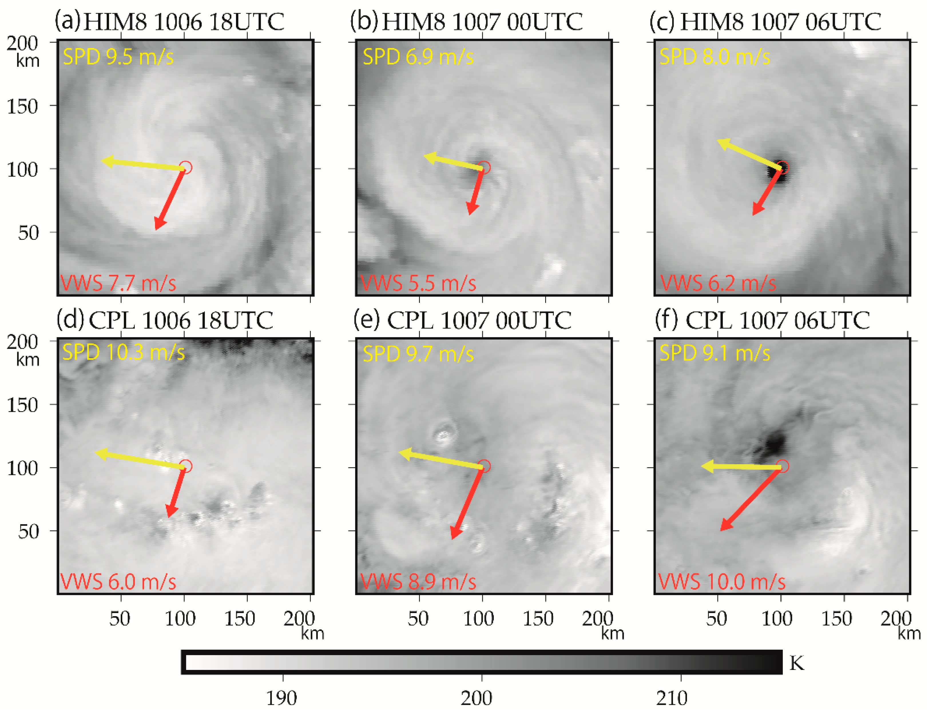
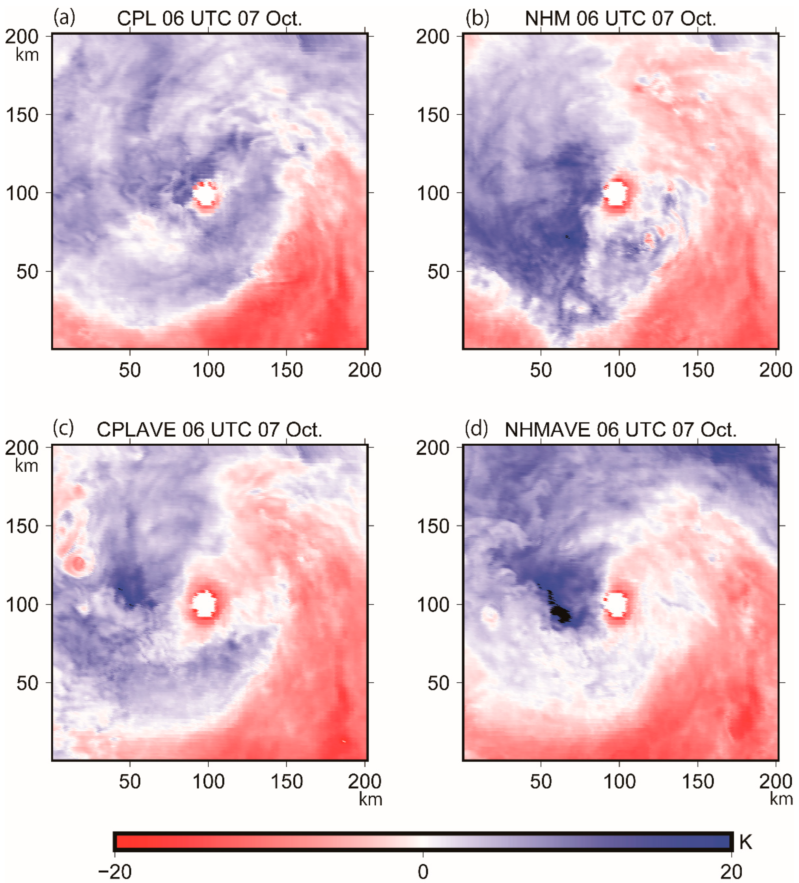
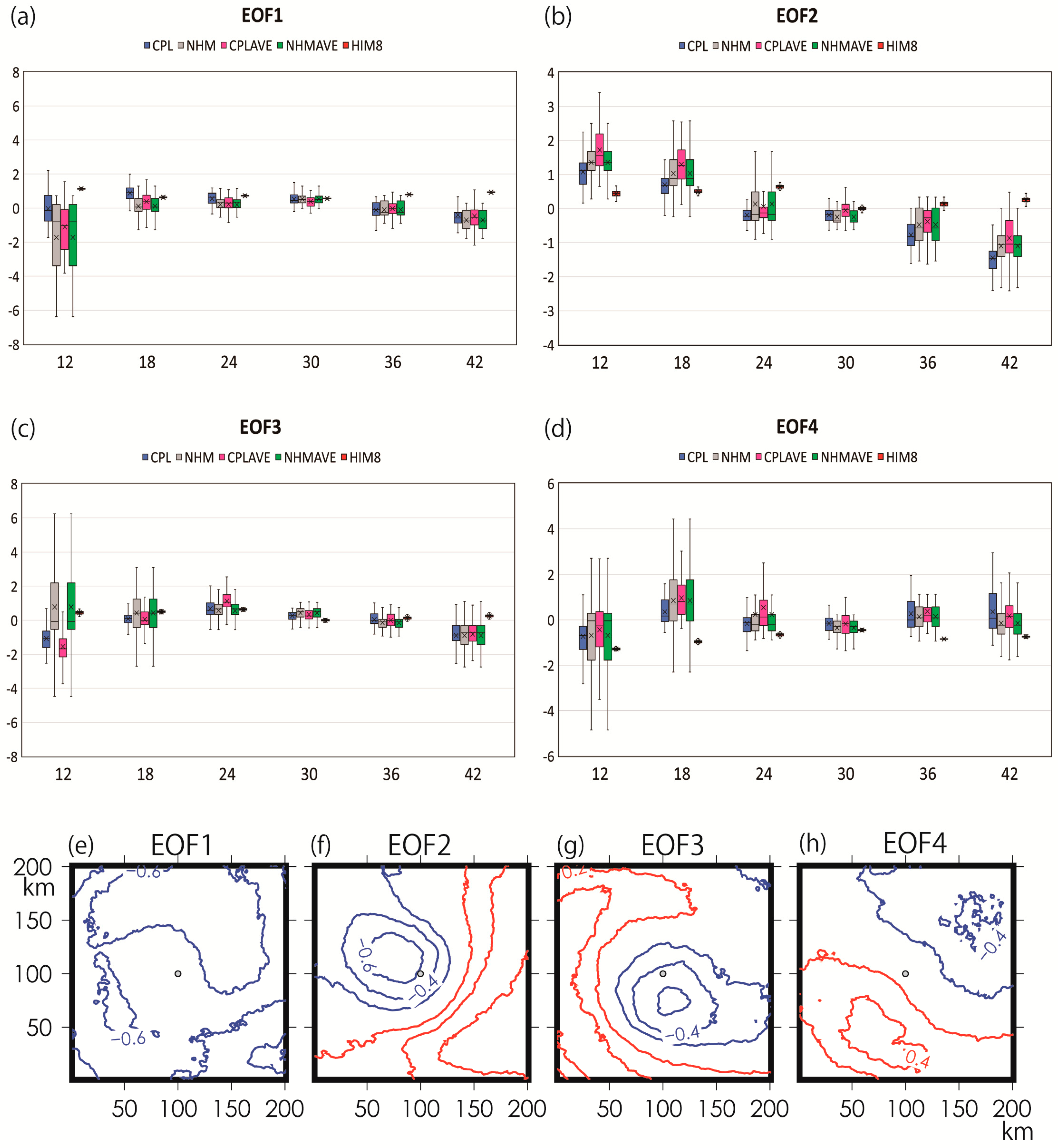
3.2. Entire Intensification Phase

The analysis period corresponds to the period from the poorly defined circulation to the eye formation of Hagibis and the cloud pattern changing from a curved band to EYE. Figure 5a–d show the time series of the normalized amplitude for the first four modes (hereafter, EOF1, EOF2, EOF3, and EOF4, respectively). Figure 5e–h show the mean variational patterns for EOF1, EOF2, EOF3, and EOF4, respectively. Each box shows a range of normalized amplitudes from the 25th percentile to 75th percentile, with the lowest and highest data points in each ensemble simulation excluding any outliers. ‘X’ indicates the mean value and ‘−’ indicates the median. Blue, gray, magenta, and green colors show the results of IR BT of b13 simulated by RTTOV with the CPL, NHM, CPLAVE, and NHMCPL ensemble simulations, respectively. Red color with a black edge shows the results of Himawari–8 IR BT of b13. The normalized amplitude for the results of Himawari–8 IR BT of b13 was almost the same for 100 trials. The first four modes account for 30.1% for EOF1, 18.7% for EOF2, 11.0% for EOF3, and 7.1% for EOF4 of the total variation as an average of 100 times (thus, the number of samples was 16,200 in each experiment and 600 in the Himawari–8 observation), and the total accounts for 66.9% of the total variation. Each mode was not contaminated by adjacent modes based on [45].
Figure 5e shows that EOF1 had a pattern with the same sign in the entire domain, while Figure 5f–h show that EOF2–4 had the wavenumber 1 asymmetric pattern, which was different from each other. At 12 h, the normalized amplitude of Himawari–8 EOF1 was out of the box range in all ensemble simulations, even though any box range of the normalized amplitude was relatively large. The normalized amplitude of Himawari–8 EOF1 remained positive from 12 h to 42 h, but the sign from the 25th percentile to 75th percentile in all ensemble simulations roughly changed from negative to positive values from 12 h to 30 h and then changed to negative values at 42 h. In particular, the sign of the EOF1 normalized amplitude from the 25th percentile to 75th percentile in all ensemble simulations was different from that of Himawari–8 at 12 h and 42 h. The difference at 42 h indicates that TC intensification represented by reduction in Himawari–8 IR BT of b13 could not be simulated in all ensemble simulations. If a very few members can simulate the Himawari–8 EOF1 variation, it may be considered as an outlier for most ensemble simulations.
Figure 5f shows a similar pattern to Figure 5g in that the sign of the EOF2–3 variational patterns at around the TC center differed from that in the outwardly spiraling area. The EOF2 pattern showed negative ahead of the moving direction and positive behind of it. However, the tendency of EOF2 normalized amplitude shown in Figure 5b differed from that of EOF3 in Figure 5c in that the sign of the EOF2 normalized amplitude from the 25th percentile to 75th percentile changed monotonically from positive to negative as the integration time progressed (Figure 5b). This tendency of the EOF2 normalized amplitude also quite differed from that of Himawari–8 at 12 h and 42 h, implying that the TC translation (speed of TC motion and its direction) differed between the best tracks and simulated tracks. In Figure 5c, the time variation of EOF3 normalized amplitude was not so large, except at 12 h. The normalized amplitude in the ensemble simulations showed a clear difference from that of Himawari–8 only at 42 h. At 12 h, the effect of ocean coupling on the variation in the EOF3 normalized amplitude was clearly seen.
Figure 5h showed a pattern with different signs along the moving direction of TC, which was associated with VWS (Figure 3). As shown in Figure 5d, the simulated EOF4 normalized amplitudes at 18 h and 36 h were significantly different from those of Himawari–8. Although the decreases in the simulated IR BT of b13 that appeared on the upshear side were consistent with the previous studies [23,24], the sign of the Himawari–8 normalized amplitude differed from the previous studies [23,24] and remained negative. This suggests that the dynamic and thermodynamic processes obtained from numerical simulations could not always explain the intensification and structural changes of real TC.

3.3. Early Intensification Phase

The early intensification phase corresponds to the period of the strengthening of clear circulation around the TC center. At 27 h, the cloud pattern of real Hagibis became EYE. The first four modes accounted for 33.8% for EOF1, 17.5% for EOF2, 10.5% for EOF3, and 5.6% for EOF4 of the total variation as an average of 100 times, respectively. The total accounted for 67.4% of the total variation without any contamination between the modes [45]. In Figure 6a, the sign of the Himawari–8 EOF1 normalized amplitude remained positive, while the simulation results had an increasing trend of the normalized amplitude going from negative to positive during 12–18 h. At 12 h, the range of normalized amplitude was broader than the range at the other integration times, indicating that the mode pattern was not stable and was still affected by external conditions such as atmospheric and oceanic conditions at 0 h to some extent.
The tendency of the normalized amplitude in Figure 6b quite differed from that in Figure 6a in that it appeared to change the sign from positive to negative particularly in the CPL and CPLAVE experiments, although the sign of the Himawari–8 normalized amplitude remained positive, except at 42 h. At 18 h and 24 h, the value of the EOF2 normalized amplitude in the ensemble simulations became close to that of Himawari–8. In Figure 6c, in contrast, the value of the EOF3 normalized amplitude in the ensemble simulations became abnormally higher than that of Himawari–8 during 18–24 h. In Figure 6d, the normalized amplitude of Himawari–8 was lower than the EOF4 normalized amplitude in the ensemble simulations, except at 15 h.
The effect of ocean coupling, represented by the difference in the normalized amplitude between the CPL and NHM experiments and between the CPLAVE and NHMAVE experiments, was clearly seen only at 12 h in the EOF2 (Figure 6b), EOF3 (Figure 6c), and EOF4 (Figure 6d) modes, which was a little different from that in the EOF3 mode in the entire intensification phase (Figure 5c). However, there is no effect of the oceanic initial condition on the evolution of the normalized amplitude in the ensemble simulations, unlike the result of the idealized numerical experiment [46]. From the idealized numerical experiment, a relatively low water temperature at 0 h and sea surface cooling caused by ocean coupling led to delaying the formation of a ring–like potential vorticity pattern in the inner core, resulting in suppression of RI [46]. In other words, the effect of ocean coupling was robust in the spin–up (early intensification) phase of TC, when the inertial stability in the upper troposphere remained small, the horizontal scale of the TC was relatively large, and the divergence was weakly counterclockwise. Although ocean coupling affected the axisymmetrization process from the asymmetric pattern, it is inferred that it was not essential for the EOF1 variational pattern and its associated TC intensification.
Figure 6e shows a similar EOF1 variational pattern to Figure 5e in that the sign was negative over all of the 200 km × 200 km domain. This indicates that the TC intensification shown in the Himawari–8 EOF1 mode could not be well simulated in the early integration time, particularly at 12 h. When considering the sign of the variance together with the EOF normalized amplitude, Figure 6f was similar to Figure 5f in that the sign of the EOF2 variational pattern showed negative ahead of the moving direction and positive behind of it. However, the difference between Figure 5f and Figure 6f existed near the TC center. Figure 6f showed an asymmetric spiral pattern, which differed from a monopole negative–sign area in Figure 5f. The negative EOF2 normalized amplitude (Figure 6b) with the positive variational pattern (Figure 6f), particularly at 15 h, possibly indicated the northwestward shift of simulated TC tracks. The EOF3 pattern in Figure 6g quite differed from that in Figure 5g. The simulated VWS in the CPL control experiment was 6.0 m s−1 at 18 h, the smallest in Figure 3d–f. The difference in the VWS possibly affected the difference in the EOF4 pattern between Figure 5h and Figure 6h, namely the difference between the entire and early intensification phases. Relatively low VWS at 18 h in the CPL experiment led to a monopole pattern in the vicinity of the TC center (Figure 6h), while relatively high VWS at 30 h in the CPL experiment led to an asymmetric pattern (Figure 5h).

3.4. Late Intensification Phase

The late intensification phase corresponds to the formation period of the TC eye. The first four modes accounted for 33.2% for EOF1, 12.3% for EOF2, 10.1% for EOF3, and 7.8% for EOF4 of the total variation as an average of 100 times, respectively. The total accounted for 63.4% of the total variation without any contamination between the modes [45]. In Figure 7a, the sign of the Himawari–8 EOF1 normalized amplitude remained positive during 27–42 h, while the sign of the EOF1 normalized amplitude in the ensemble simulations changed from positive to negative during 33−39 h. This suggests that TC intensification implied by the Himawari–8 EOF1 normalized amplitude could not be simulated in all ensemble simulations after 36 h, which was consistent with the result shown in Figure 2b in that the simulated TC intensification had been suppressed after 36 h.
In contrast, the Himawari–8 EOF2 normalized amplitude was consistent with that in the ensemble simulations after 39 h (Figure 7b). In addition, the Himawari–8 EOF3 normalized amplitude was roughly consistent with that in the ensemble simulations at 42 h. The results on the normalized amplitude after 39 h in the EOF2 and EOF3 modes was different from that in the EOF1 mode. With respect to Figure 7d, the Himawari–8 EOF4 normalized amplitude was consistent with that in all ensemble simulations, but the box range from the 25th percentile to 75th percentile became wide, particularly at 30 h and 33 h. This suggests that the Himawari–8 EOF4 normalized amplitude at 30 h and 33 h depended on how the ensemble members were selected. In other words, there may be more uncertainty in the EOF4 mode, particularly at 30 h and 33 h, due to atmospheric and oceanic initial conditions than at the other integration times.
In Figure 7e, the EOF1 variational pattern was monopole. The result further emphasized the results of Figure 5e on the fact that the TC intensification, represented by reduction in the Himawari–8 IR BT of b13, could not be simulated in all ensemble simulations. From the comparison between Figure 5f and Figure 6f, the EOF2 variational pattern in Figure 7f clearly showed a north–northwest to south–southeast wavenumber–1 asymmetric pattern. Since the Himawari–8 normalized amplitude alternatively changed the sign, however, the role of the EOF2 mode in TC translation did not become clear in the late intensification phase. In contrast, Figure 7g shows an east–west asymmetric pattern with different signs, being consistent with the direction of TC motion (Figure 3). Figure 7h differed from the previous EOF variational patterns in that the absolute value of the variance was lower than 0.2 over all of the 200 km × 200 km domain, an indication that the variance in the EOF4 mode was not significant, although the contrast of the variance at the eye to that outside of the eye seemed to be clear in Figure 7h. The wide box range of the Himawari–8 IR BT of b13 from the 25th percentile to 75th percentile during 30–33 h (Figure 7d) may be caused by the presence or absence of strong, sporadic convection in the vicinity of the eye which occurred in the late intensification phase. In order to stably extract representative mode for strong sporadic convection, such as convective burst [24,47], it will be necessary to perform EOF calculations for higher time–resolving data than 3 h.

3.5. Prediction by Multiple Linear Regression Analysis

We have described the features of the first four EOF modes at around the TC center obtained from the EOF analysis with the Himawari–8 IR BT of b13 and the IR BT of b13 simulated by RTTOV with the results of the CPL, NHM, CPLAVE, and NHMAVE experiments. In this section, multiple linear regression analysis was conducted for the normalized amplitude of the first four EOF modes and the corresponding 6 h simulated central pressure tendencies. Then, the multiple linear regression equation was applied for the Himawari–8 normalized amplitude to estimate the Himawari–8 6 h central pressure tendency.
Figure 8a shows the timeseries of 6 h central pressure tendency in the CPL, NHM, CPLAVE, and NHMAVE experiments in the entire intensification phase (from 12 h to 42 h). Figure 8b shows the timeseries of 6 h central pressure tendency in the ensemble simulations estimated by the multiple linear regression equation in the same entire intensification phase. In Figure 8a, the RSMC–Tokyo and JTWC best–track central pressure tendencies are shown along with the simulation results, although the 6 h tendency was calculated in the previous 6 h. In Figure 8b, the Himawari–8 6 h central pressure tendency is shown along with the results calculated by the multiple linear regression equation based on the simulated normalized amplitude. Figure 8c,d is the same as Figure 8a,b, except in the early intensification phase (from 12 h to 27 h), and Figure 8e,f is in the late intensification phase (from 27 h to 42 h). It should be noted that the 6 h central pressure tendency in the ensemble simulations was calculated as a difference in simulated central pressures between 3 h before and after the specified integration time, which was different from the two best–track tendencies. The period for calculating the difference in simulated central pressures was set to 3 h before and after the specified integration time because of the removal of the effect of the initial conditions in the early integration phase as much as possible. At 12 h, 24 h, and 42 h, the 6 h central pressure tendency estimated from the Himawari–8 normalized amplitude was below the box range from the 25th percentile to 75th percentile in each ensemble simulation (Figure 8b). This suggests that the Himawari–8 6 h central pressure tendency was not adequately reproduced in all ensemble simulations at 12 h, 24 h, and 42 h, respectively. The box range of the tendency was reduced when the tendency was estimated by the multiple linear regression equation (Figure 8b). The reduction was resulted from the fact that the variation in simulated 6 h tendency among the ensemble simulations was reduced due to a result of the linear approximation by the introduction of the multiple linear regression equation. Nevertheless, the Himawari–8 6 h central pressure tendency at 12 h and 42 h was not adequately reproduced by the multiple linear regression equation with the Himawari–8 normalized amplitude in the first four EOF modes.
When the analysis period was separated into the early and late intensification phases and multiple linear regression analysis was conducted for each phase, the difference in 6 h central pressure tendency between the ensemble simulation and the Himawari–8 estimates by multiple linear regression analysis was more obvious at 12 h in the early intensification phase and at 39 h and 42 h in the late intensification phase. In other words, for the other integration times, the 6 hourly central pressure tendency in the ensemble simulations was consistent with that the Himawari–8 6 h central pressure tendency estimated by the multiple linear regression equation. Using the estimated 6 h central pressure tendency as a reference, in the following, we can discuss the validity of RSMC–Tokyo and JTWC best–track central pressure tendency (Figure 8a).
At 12 h, the central pressure in the ensemble simulations was shallower than that of the two best tracks (Figure 8a,c). However, the RSMC–Tokyo best–track central pressure (−15 hPa/6 h) may be too deep compared to the Himawari–8 estimate (−6.2 hPa/6 h). After 36 h, on the other hand, the JTWC best–track central pressure showed an increasing tendency (+19 hPa/6 h), while the Himawari–8 estimate showed a decreasing tendency (−6.0 hPa/6 h) (Figure 8a,e). Since the RSMC–Tokyo best–track central pressure kept the value of 915 hPa, the Himawari–8 estimate was closer to the RSMC–Tokyo best–track central pressure tendency than the JTWC one. It should be noted that the simulation results may be affected by the initial conditions in the early integration time (at 12 h) and by the lateral boundaries in the late integration time (after 36 h). If the model domain is taken to be broader, the results, especially in the latter integration time, may change.
The difference in the central pressure between RSMC–Tokyo and JTWC (Figure 8a,c,e) may be attributed to the differences in the TC current intensity (CI) number estimated by the Dvorak technique. Alternatively, if the CI number is the same as that of RSMC–Tokyo, the difference may be attributed to the difference of the convert table from the CI number to the central pressure between RSMC–Tokyo and JTWC [42].

4. Discussion

Ensemble TC forecasting, based on weather forecasting models with different atmospheric conditions at the initial time, has been utilized by some operational centers to improve the accuracy of TC track forecasts [8]. However, its application to TC intensity forecasting has been considered premature and challenging, partly due to the poor reproduction of the TC central pressure and maximum surface wind speed (attributed to poor model specifications and its configuration) [11]. Since aircraft in situ observations are not operational in the Northwestern Pacific, TC intensity analysis using geostationary satellite data and the Dvorak technique has been believed to be the most reliable, even now [14]. A deep–learning model using satellite imagery, such as a conventional convolutional neural network [48], has been recently developed to objectively estimate TC intensity. Nevertheless, as shown in Figure 2b, the best–track data based on the Dvorak method sometimes differed from the best–track archives [42]. The Hagibis’s case is exactly that the JTWC tends to estimate faster intensification rates before the mature phase than RSMC–Tokyo [42]. The discrepancies between best–track datasets do affect the validation of TC intensity analysis and forecast.
If TC intensity, such as minimum sea–level pressure and maximum surface wind speed, is directly estimated from the Himawari–8 IR BT of b13 in a more objective manner than the Dvorak technique, the relation between the Dvorak pattern and TC intensity would be understood in a dynamic and thermodynamic sense. The IR BT of b13 calculated by RTTOV with the ensemble simulation is closely associated with various physical components and quantities; therefore, it would be possible to retrieve the quantities of the physical components from the Himawari–8 IR BT of b13 by using the simulation results or by multiple linear regression function equation based on the representative EOF modes without any contamination among the modes. However, the results of this study also indicate that the normalized amplitude of the representative modes on the Himawari–8 IR BT of b13 can occasionally be an outlier among the ensemble simulations. This suggests that, at specified integration times, the numerical model used in this study could not reproduce the real TC structure that is closely associated with TC intensity estimates based on the Himawari–8 IR BT of b13 and the Dvorak technique. Moreover, the differences in simulation results caused by ocean coupling and different oceanic initial conditions have little effect on modifying the representative first EOF modes of IR BT of b13 associated with TC intensity estimates in the intensification phase, except at 12 h. In particular, the oceanic preexisting conditions do not inherently affect the representative EOF mode. Therefore, the role of ocean coupling, and oceanic preexisting condition is only quantitative (Figure 2b), which is explained by the fact that the ocean does affect the TC intensity through TC secondary circulation [31]. The role of ocean coupling and oceanic preexisting condition is not essential with respect to structural changes in the late intensification phase.
The ratio of the explainable variance, from the representative modes to the overall variance, is expected to vary depending on the calculation domain and the spatiotemporal resolution of the IR BT of b13 or the other band channel of Himawari–8, which would affect the interpretation presented in this study. For example, the role of strong convection on TC intensification implied by the EOF4 mode (Figure 7d,h) remained uncertain in this study. In other words, by preparing the Himawari–8 and simulated IR BT of b13 data that match the spatiotemporal resolution of the targeted variability and applying the EOF analysis for a more appropriate domain, it would be possible to determine the representative modes associated with dynamics and thermodynamics around the TC center that are beyond the scope of this study. This will contribute to identifying the weaknesses of the numerical model and its physical processes and thereby develop strategies for improvement.

5. Conclusions

An ensemble simulation has become a mainstream method in stochastic TC forecasting and projecting with the improvement of computer technology [8]. However, due to the extremely large amount of output data, only a fraction of information included in the output has been utilized so far. PC (or EOF) analysis is a method that can extract representative modes from the extremely large data by linear mode expansion so as to explain the largest variance associated with internal variability in the atmosphere and ocean, although the representative modes are not necessarily connected with physical processes and we do not know whether the large ensemble includes the correct answer that is supported by observational evidence, such as the Himawari–8 IR BT of b13 [17], which is usually utilized as TC intensity estimates by the Dvorak technique [12,14].
In the present study, an EOF analysis was performed for the inner core of Hagibis in the intensification phase. The Himawari–8 IR BT collocated at the Hagibis’s center was combined with the IR BT simulated by RTTOV with 1 km ensemble simulations conducted by NHM and CPL, with two different oceanic initial condition under one control atmospheric initial condition and the 26 perturbed ones. The representative first four EOF modes showed symmetric and asymmetric patterns in the inner core, which enabled explanation of the curved band, CDO, and EYE pattern used as classification patterns in the Dvorak technique. This indicates that the ensemble simulation could reproduce the representative cloud patterns observed by the Himawari–8 in the intensification phase of Hagibis, irrespective of ocean warming and ocean coupling. Since the negative sign of the EOF1 variational pattern over all of the 200 km × 200 km domain collocated at the TC center indicates that the IR BT is lowering, the EOF1 mode represents TC intensification. The result of the normalized amplitude of the Himawari–8 IR BT suggests that Hagibis underwent intensification from 6 to 7 October in 2019. In the late intensification phase (at 39 h and 42 h), however, TC intensification represented by the Himawari–8 IR BT of b13 could not be simulated in all ensemble simulations. Nevertheless, the results of ensemble simulations could reproduce the ‘real’ cloud patterns of Himawari–8 in the intensification phase of Hagibis to some extent.
The EOF2 mode showed the wavenumber–1 asymmetric pattern that was related to TC translation, particularly in the early intensification phase. The pattern was characterized by a different sign between the forward and backward side of the TC translation and between the right and left sides of VWS. The EOF3–4 variational patterns showed the similar wavenumber–1 asymmetric pattern, but the different sign seems to appear between the upshear and downshear sides. In the late intensification phase, the EOF3 mode was related to TC translation instead of the EOF2 mode. Although many insights into the wavenumber–1 asymmetric pattern and TC translation have been obtained in this study, the role of the wavenumber–1 asymmetry in TC intensification and structural changes was uncertain due to inconsistency with the previous study [23,24]. The uncertainty is partly attributed to insufficient spatiotemporal resolution of the IR BT of b13 data used in the present study so that the role of strong sporadic convection, such as convective bursts on TC intensification, could not be captured and is beyond the scope of this study. Therefore, the dynamic and thermodynamic processes associated with TC intensification and structural changes of real TC are still not fully explained in this study, except for the role of ocean coupling and oceanic preexisting conditions.
The influence of ocean coupling first appeared at 12 h on the EOF modes associated with the wavenumber–1 asymmetry, but the impact was relatively small compared to the difference between the Himawari–8 observations and ensemble simulations. While ocean coupling and the difference in oceanic preexisting conditions could quantitatively affect the IR BT of b13 in the TC inner core through the secondary circulation [31], the normalized amplitude did not become close to that of the Himawari–8 observation, an indication that the inner–core representative EOF mode could not be essentially affected by altering the oceanic initial condition and using the atmosphere–wave–ocean coupled model. In other words, except for the quantitative effects, the inner–core dynamics and thermodynamics of Hagibis associated with its structural change were not affected by the oceanic preexisting condition and ocean coupling, except at 12 h.
Using the normalized amplitudes in the first four EOF modes, a multiple linear regression analysis was conducted for 6 h simulated central pressure tendencies and the normalized amplitude in all ensemble simulations and the Himawari–8′s normalized amplitude to estimate the Himawari–8 6 h central pressure tendency. The simulated central pressure tendency was characterized by relatively small decreases in the central pressure in the early (at 12 h) and late (after 36 h) intensification phase when compared with the RSMC–Tokyo and JTWC best–track central pressure tendency, as well as the Himawari–8 tendency, estimated from the multiple linear regression equation. This is consistent with the features inferred from the time series of the normalized amplitude and the EOF variational pattern. It should be noted, however, that the simulation results were affected by the lateral boundaries in the late intensification phase, as well as the initial conditions in the early intensification phase, because of the usage of a regional atmosphere model.
The next step is to apply this EOF analysis for the other physical components such as tangential, radial winds, and potential vorticity in the lower troposphere and potential temperature in the upper troposphere and then evaluate the correspondence of the representative modes of Himawari–8 IR BT of b13. In addition, we need to study how the differences in the physical processes in the NHM, particularly cloud microphysics, affect the representative EOF modes of Himawari–8 IR BT of b13, TC intensification, and the structural changes. This will serve as an improvement to the numerical model for TC forecasting.

Author Contributions

Conceptualization, A.W.; data curation, A.W.; formal analysis, A.W.; funding acquisition, A.W., M.H. and W.Y.; investigation, A.W.; methodology, A.W. and M.H.; project administration, A.W. and W.Y.; resources, A.W., M.H. and W.Y.; software, A.W. and M.H.; supervision, A.W.; validation, A.W.; visualization, A.W.; writing—original draft preparation, A.W.; writing—review and editing, A.W., M.H. and W.Y. All authors have read and agreed to the published version of the manuscript.

Funding

This research was funded by Grants–in–Aid for Scientific Research (JP22K03725, JP18K03747, and JP19H05696) from the Japan Society for the Promotion of Science.

Informed Consent Statement

Not applicable.

Data Availability Statement

The RSMC–Tokyo and JTWC best–track data, RTTOV, and remote sensing systems SST were downloaded from the websites listed in ‘References’. Some of the datasets and program codes used in this study are not publicly available due to the management policy of the Japan Meteorological Agency (JMA) (http://pfi.kishou.go.jp/ (accessed on 22 August 2022) (in Japanese)) but may be available from the first author for reasonable usage upon request. All rights remain with the JMA.

Acknowledgments

The author appreciates three anonymous reviewers for their comments which help improve the first manuscript. Generic Mapping Tools software (https://www.soest.hawaii.edu/gmt/ (accessed on 22 August 2022)) was used to draw the figures.

Conflicts of Interest

The authors declare no conflict of interest.

References

  1. Thompson, D.W.J.; Wallace, J.M. The Arctic oscillation signature in the wintertime geopotential height and temperature fields. Geophys. Res. Lett. 1998, 25, 1297–1300. [Google Scholar] [CrossRef]
  2. Kikuchi, K. Extension of the bimodal intraseasonal oscillation index using JRA–55. Clim. Dyn. 2020, 54, 919–933. [Google Scholar] [CrossRef]
  3. Wheeler, M.C.; Hendon, H.H. An all–season real–time multivariate MJO index: Development of an index for monitoring and prediction. Mon. Wea. Rev. 2004, 132, 1917–1932. [Google Scholar] [CrossRef]
  4. Zheng, M.; Chang, E.K.M.; Colle, B.A.; Luo, Y.; Zhu, Y. Applying fuzzy clustering to a multimodel ensemble for U.S. East Coast winter storms: Scenario identification and forecast verification. Wea. Forecast. 2017, 32, 881–903. [Google Scholar] [CrossRef]
  5. Zheng, M.; Chang, E.K.M.; Colle, B.A. Evaluating U.S. East Coast winter storms in a multimodel ensemble using EOF and clustering approaches. Mon. Wea. Rev. 2019, 147, 1967–1987. [Google Scholar] [CrossRef]
  6. Wada, A.; Chan, J.C.L. Increasing TCHP in the western North Pacific and its influence on the intensity of FAXAI and HAGIBIS in 2019. SOLA 2021, 17A, 29–32. [Google Scholar] [CrossRef]
  7. Wada, A. Atmosphere–Wave–Ocean Coupled–Model Ensemble Simulation on Rapid Intensification of Typhoon Hagibis (2019). WGNE Res. Activ. Earth Sys. Modell. 2021, 51, 9–07–9–08. [Google Scholar]
  8. Heming, J.; Prates, F.; Bender, M.A.; Bowyer, R.; Cangialosi, J.; Caroff, P.; Coleman, T.; Doyle, J.D.; Dube, A.; Faure, G.; et al. Review of recent progress in tropical cyclone track forecasting and expression of uncertainties. Trop. Cyclone Res. Rev. 2019, 8, 181–218. [Google Scholar] [CrossRef]
  9. Yamaguchi, M.; Ishida, J.; Sato, H.; Nakagawa, M. WGNE Intercomparison of tropical cyclone forecasts by operational NWP Models: A quarter century and beyond. Bull. Amer. Meteor. Soc. 2017, 98, 2337–2349. [Google Scholar] [CrossRef]
  10. Emanuel, K.; Zhang, F. The role of inner–core moisture in tropical cyclone predictability and practical forecast skill. J. Atmos. Sci. 2017, 74, 2315–2324. [Google Scholar] [CrossRef]
  11. Wang, Y.; Wu, C.C. Current understanding of tropical cyclone structure and intensity changes—A review. Meteorol. Atmos. Phys. 2004, 87, 257–278. [Google Scholar] [CrossRef]
  12. Dvorak, V.F. Tropical cyclone intensity analysis using satellite data. NOAA Tech. Rep. 1984, 11, 45. [Google Scholar]
  13. Olander, T.L.; Velden, C.S. The advanced Dvorak technique (ADT) for estimating tropical cyclone intensity: Update and new capabilities. Wea. Forecast. 2019, 34, 905–922. [Google Scholar] [CrossRef]
  14. Velden, C.; Harper, B.; Wells, F.; Beven, J.L.; Zehr, R.; Olander, T.; Mayfield, M.; Guard, C.; Lander, M.; Edson, R.; et al. The Dvorak tropical cyclone intensity estimation technique: A satellite–based method that has endured for over 30 years. Bull. Amer. Meteor. Soc. 2006, 87, 1195–1210. [Google Scholar] [CrossRef]
  15. Oyama, R.; Nagata, K.; Kawada, H.; Koide, N. Development of a product based on consensus between Dvorak and AMSU tropical cyclone central pressure estimates at JMA. RSMC Tokyo–Typhoon Cent. Tech. Rev. 2016, 18, 1–8. [Google Scholar]
  16. Sasaki, H.; Motoi, T. Accelerated Increase in Tropical Cyclone Heat Potential in the Typhoon Rapidly Intensifying Zone during 1955–2020. SOLA 2022, 18, 65–70. [Google Scholar] [CrossRef]
  17. Bessho, K.; Date, K.; Hayashi, M.; Ikeda, A.; Imai, T.; Inoue, H.; Kumagai, Y.; Miyakawa, T.; Murata, H.; Ohno, T.; et al. An introduction to Himawari–8/9—Japan’s new–generation geostationary meteorological satellites. J. Meteor. Soc. Jpn. 2016, 94, 151–183. [Google Scholar] [CrossRef]
  18. Merrill, R.T. Environmental influences on hurricane intensification. J. Atmos. Sci. 1988, 45, 1678–1687. [Google Scholar] [CrossRef]
  19. Kaplan, J.; DeMaria, M. Large–scale characteristics of rapidly intensifying tropical cyclones in the North Atlantic basin. Wea. Forecast. 2003, 18, 1093–1108. [Google Scholar] [CrossRef]
  20. Hendricks, E.A.; Peng, M.S.; Fu, B.; Li, T. Quantifying environmental control on tropical cyclone intensity change. Mon. Wea. Rev. 2010, 138, 3243–3271. [Google Scholar] [CrossRef]
  21. Rios–Berrios, R.; Torn, R.D. Climatological analysis of tropical cyclone intensity changes under moderate vertical wind shear. Mon. Wea. Rev. 2017, 145, 1717–1738. [Google Scholar] [CrossRef]
  22. Harnos, D.S.; Nesbitt, S.W. Convective structure in rapidly intensifying tropical cyclones as depicted by passive microwave measurements. Geophys. Res. Lett. 2011, 38, L07805. [Google Scholar] [CrossRef]
  23. Shi, D.; Chen, G. The implication of outflow structure for the rapid intensification of tropical cyclones under vertical wind shear. Mon. Wea. Rev. 2021, 149, 4107–4127. [Google Scholar] [CrossRef]
  24. Fischer, M.S.; Tang, B.H.; Corbosiero, K.L.; Rozoff, C.M. Normalized convective characteristics of tropical cyclone rapid intensification events in the North Atlantic and Eastern North Pacific. Mon. Wea. Rev. 2018, 146, 1133–1155. [Google Scholar] [CrossRef]
  25. Rios–Berrios, R.; Davis, C.A.; Torn, R.D. A hypothesis for the intensification of tropical cyclones under moderate vertical wind shear. J. Atmos. Sci. 2018, 75, 4149–4173. [Google Scholar] [CrossRef]
  26. Tao, D.; Zhang, F. Evolution of dynamic and thermodynamic structures before and during rapid intensification of tropical cyclones: Sensitivity to vertical wind shear. Mon. Wea. Rev. 2019, 147, 1171–1191. [Google Scholar] [CrossRef]
  27. Dai, Y.; Majumdar, S.J.; Nolan, D.S. Tropical cyclone resistance to strong environmental shear. J. Atmos. Sci. 2021, 78, 1275–1293. [Google Scholar] [CrossRef]
  28. Hardy, S.; Schwendike, J.; Smith, R.K.; Short, C.J.; Reeder, M.J.; Birch, C.E. Fluctuations in inner–core structure during the rapid intensification of super typhoon Nepartak (2016). Mon. Wea. Rev. 2021, 149, 221–243. [Google Scholar] [CrossRef]
  29. RSMC Tokyo–Typhoon Center Best Track Data. Available online: https://www.jma.go.jp/jma/jma–eng/jma–center/rsmc–hp–pub–eg/trackarchives.html (accessed on 22 August 2022).
  30. Naval Oceanography Portal Tropical Cyclone Support Best Track Archive. Available online: https://www.metoc.navy.mil/jtwc/jtwc.html?best–tracks (accessed on 22 August 2022).
  31. Wada, A.; Kanada, S.; Yamada, H. Effect of air–sea environmental conditions and interfacial processes on extremely intense typhoon Haiyan (2013). J. Geophys. Res. Atmos. 2018, 123, 10379–10405. [Google Scholar] [CrossRef]
  32. Ikawa, M.; Saito, K. Description of a nonhydrostatic model developed at the forecast research department of the MRI. Tech. Rep. MRI 1991, 28, 238. [Google Scholar] [CrossRef]
  33. Lin, Y.L.; Farley, R.D.; Orville, H.D. Bulk parameterization of the snow field in a cloud model. J. Appl. Meteor. Climatol. 1983, 22, 1065–1092. [Google Scholar] [CrossRef]
  34. Kondo, J. Air–sea bulk transfer coefficients in diabatic conditions. Bound. Layer Meteor. 1975, 9, 91–112. [Google Scholar] [CrossRef]
  35. Taylor, P.K.; Yelland, M.J. The dependence of sea surface roughness on the height and steepness of the waves. J. Phys. Oceanogr. 2001, 31, 572–590. [Google Scholar] [CrossRef]
  36. Klemp, J.B.; Wilhelmson, R. The simulation of three–dimensional convective storm dynamics. J. Atmos. Sci. 1978, 35, 1070–1096. [Google Scholar] [CrossRef]
  37. Deardorff, J.W. Stratocumulus–capped mixed layers derived from a three–dimensional model. Bound. Layer Meteor. 1980, 18, 495–527. [Google Scholar] [CrossRef]
  38. Sugi, M.; Kuma, K.; Tada, K.; Tamiya, K.; Hasegawa, N.; Iwasaki, T.; Yamada, S.; Kitade, T. Description and performance of the JMA operational global spectral model (JMA–GSM88). Geophys. Mag. 1990, 43, 105–130. [Google Scholar]
  39. Remote Sensing Systems Measurement Sea Surface Temperature. Available online: https://www.remss.com/measurements/sea–surface–temperature (accessed on 22 August 2022).
  40. Usui, N.; Wakamatsu, T.; Tanaka, Y.; Hirose, N.; Toyoda, T.; Nishikawa, S.; Fujii, Y.; Takatsuki, Y.; Igarashi, H.; Nishikawa, H.; et al. Four–dimensional variational ocean reanalysis: A 30–year high–resolution dataset in the western North Pacific (FORA–WNP30). J. Oceanogr. 2017, 73, 205–233. [Google Scholar] [CrossRef]
  41. Eumetsat NWP SAF RTTOV v13. Available online: https://nwp–saf.eumetsat.int/site/software/rttov/rttov–v13/ (accessed on 22 August 2022).
  42. Nakazawa, T.; Hoshino, S. Intercomparison of Dvorak parameters in the tropical cyclone datasets over the western North Pacific. SOLA 2009, 5, 33–36. [Google Scholar] [CrossRef]
  43. Atcf Tropical Cyclone Database. Available online: https://www.nrlmry.navy.mil/atcf_web/docs/database/new/database.html (accessed on 22 August 2022).
  44. Kitabatake, N.; Hoshino, S.; Sakuragi, T. Estimation of tropical cyclone intensity using TRMM/TMI brightness temperature data with asymmetric components. Pap. Meteor. Geophys. 2014, 65, 57–74. [Google Scholar] [CrossRef]
  45. North, G.R.; Bell, T.L.; Cahalan, R.F.; Moeng, F.J. Sampling errors in the estimation of empirical orthogonal functions. Mon. Wea. Rev. 1982, 110, 699–706. [Google Scholar] [CrossRef]
  46. Wada, A. Idealized numerical experiments associated with the intensity and rapid intensification of stationary tropical–cyclone–like vortex and its relation to initial sea–surface temperature and vortex–induced sea–surface cooling. J. Geophys. Res. Atmos. 2009, 114, D18111. [Google Scholar] [CrossRef]
  47. Horinouchi, T.; Shimada, U.; Wada, A. Convective bursts with gravity waves in tropical cyclones: Case study with the Himawari–8 satellite and idealized numerical study. Geophys. Res. Lett. 2020, 47, e2019GL086295. [Google Scholar] [CrossRef]
  48. Chen, B.; Chen, B.; Lin, H.; Elsberry, R.L. Estimating tropical cyclone intensity by satellite imagery utilizing convolutional neural networks. Wea. Forecast. 2019, 34, 447–465. [Google Scholar] [CrossRef]
Figure 1. Schematic diagram of the dataset for applying EOF analysis. The EOF analysis was conducted for the Himawari–8 IR BT and RTTOV–simulated IR BT in the CPL, NHM, CPLAVE, and NHMAVE experiments. The analysis domain was a square of 200 km × 200 km collocated at the TC Center. t indicates the integration time. n indicates the number of integration times (n = 6 in this study). The total number of data were 654 for each EOF analysis.
Atmosphere 13 01559 g001
Figure 2. (a) RSMC–Tokyo best–track, JTWC best–track, and ensemble mean simulated tracks in the NHM (gray), CPL (blue), NHMAVE (green), and CPLAVE (magenta) experiments together with simulated track in each member. Circles show the position every 3 h with colors indicating their simulated central pressure. (b) RSMC–Tokyo best–track, JTWC best–track, and ensemble mean simulated central–pressure evolution with box–and–whisker plots in the NHM, CPL, NHMAVE, and CPLAVE experiments. ‘X’ indicates the mean value and ‘−’ indicates the median. Circles with a solid line indicate the RSMC–Tokyo (black) and JTWC (red) best–track central pressure.
Atmosphere 13 01559 g002
Figure 3. Upper three panels show the horizontal distribution of Himawari–8 IR BT of b13 collocated at the RSMC–Tokyo best–track position (red open circle) (a) at 18 UTC on 6 October, (b) at 00 UTC on 7 October, and (c) at 06 UTC on 7 October in 2019 with VWS (red arrow and value). Lower three panels show the horizontal distribution of IR BT of b13 simulated with RTTOV and results of the numerical simulation in the CPL control experiment collocated at the simulated center position (d) at 18 UTC on 6 October, (e) at 00 UTC on 7 October, and (f) at 06 UTC on 7 October in 2019 with simulated VWS (red arrow and value). Yellow arrows and values indicate the moving direction and speed of Hagibis between three hours before and after the specified integration time.
Atmosphere 13 01559 g003
Figure 4. Horizontal distribution of the difference in IR BT of b13 between the Himawari–8 and the simulation by RTTOV at 06 UTC on 7 October in the (a) CPL, (b) NHM, (c) CPLAVE, and (d) NHMAVE control experiments. Cold (warm) colors indicate that the Himawari–8 IR BT of b13 was lower (higher) than the simulated IR BT of b13.
Atmosphere 13 01559 g004
Figure 5. The upper and middle box–and–whisker plots show the timeseries of the normalized amplitude from 12 h to 42 h obtained from the EOF analysis for IR BT of b13 obtained from the NHM (gray), CPL (blue), NHMAVE (green), and CPLAVE (magenta) experiments and Himawari–8 (red) in the (a) first (EOF1), (b)second (EOF2), (c) third (EOF3), and (d) fourth (EOF4) modes. The lower panels show the representative pattern of the (e) EOF1, (f) EOF2, (g) EOF2, and (h) EOF4 modes. Red shows the positive value ( 0.2 ) , whereas blue shows the negative value ( 0.2 ) .
Atmosphere 13 01559 g005
Figure 6. The upper and middle box–and–whisker plots show the timeseries of the normalized amplitude from 12 h to 27 h obtained from the EOF analysis for IR BT of b13 obtained from the NHM (gray), CPL (blue), NHMAVE (green), and CPLAVE (magenta) experiments and Himawari–8 (red) in the (a) first (EOF1), (b) second (EOF2), (c) third (EOF3), and (d) fourth (EOF4) modes. The lower panels show the representative pattern of the (e) EOF1, (f) EOF2, (g) EOF2, and (h) EOF4 modes. Red shows the positive value (≥0.2), whereas blue shows the negative value (≤−0.2).
Atmosphere 13 01559 g006
Figure 7. The upper and middle box–and–whisker plots show the timeseries of the normalized amplitude from 27 h to 42 h obtained from the EOF analysis for IR BT of b13 obtained from the NHM (gray), CPL (blue), NHMAVE (green), and CPLAVE (magenta) experiments and Himawari–8 (red) in the (a) first (EOF1), (b) second (EOF2), (c) third (EOF3), and (d) fourth (EOF4) modes. The lower panels show the representative pattern of the (e) EOF1, (f) EOF2, (g) EOF2, and (h) EOF4 modes. Red shows the positive value (≥0.1), whereas blue shows the negative value (≤−0.1).
Atmosphere 13 01559 g007
Figure 8. Timeseries of the 6 hourly simulated central pressure tendency and the tendency estimated by multiple linear regression analysis using the normalized amplitude of EOF1–4: (a) Simulation results from 12 h to 42 h every 6 h with the tendency calculated from RSMC–Tokyo and JTWC best–track archives; (b) regression results from 12 h to 42 h every 6 h; (c) simulation results from 12 h to 27 h every 3 h with the tendency of RSMC–Tokyo and JTWC best–track data every 6 h; (d) regression results from 12 h to 27 h every 3 h; (e) simulation results from 27 h to 42 h every 3 h with the tendency of RSMC–Tokyo and JTWC best–track data every 6 h; (f) regression results from 27 h to 42 h every 3 h. Central pressures of the Himawari–8 in (af) were estimated by the multiple linear analysis.
Atmosphere 13 01559 g008
Table 1. Experiment name and model physics in the atmosphere and air–sea interface.
NHMCPLNHMAVECPLAVE
modelA nonhydrostatic atmosphere modelCoupled atmosphere–wave–ocean modelA nonhydrostatic atmosphere modelCoupled atmosphere–wave–ocean model
MicrophysicsIkawa and Saito (1991) [32], Lin et al. (1983) [33]
Surface fluxKondo (1975) [34]Taylor and Yelland (2001) [35], Wada et al. (2018) [31]Kondo (1975) [34]Taylor and Yelland (2001) [35], Wada et al. (2018) [31]
TurbulenceKlemp and Wilhelmson (1978) [36], Deardorff (1980) [37]
RadiationSugi et al. (1990) [38]
Table 2. Configuration in each ensemble experiment.
NHMCPLNHMAVECPLAVE
Simulation periodFrom 00 UTC on 6 October (initial time) to 18 UTC on 7 October in 2019
Time step3 s3 s (Atmosphere), 18 s (Ocean), 6 min (Ocean wave)3 s3 s (Atmosphere), 18 s (Ocean), 6 min (Ocean wave)
Computational domain and map system1620 km x 990 km centered at 15° N, 150° E, Lambert Conformal Conic projection
Horizontal resolution and vertical layer1 km and 55 levels in vertical coordinates with intervals ranging from 40 m for the near–surface layer to 1180 m for the uppermost layer (top height is 27,440 m)
SSTMicrowave SST on 5 OctoberMicrowave SST on 5 OctoberClimatological mean microwave SST on 5 October during 1999–2018Climatological mean microwave SST on 5 October during 1999–2018
Ocean data (temperature, salinity, and current velocities)JMA mean North Pacific oceanic daily analysis on 5 OctoberClimatological mean North Pacific Ocean daily reanalysis [36] on 5 October during 1993–2018 (including JMA analysis during 2016–2018)
Atmospheric dataJMA 6 hourly global atmospheric analysis data with a horizontal grid spacing of approximately 20 km
PerturbationJMA global atmospheric ensemble prediction data with a horizontal grid spacing of 1.25° at 00 UTC on 6 October
The number of ensemble simulation1 control experiment and 26 experiments with perturbation
Publisher’s Note: MDPI stays neutral with regard to jurisdictional claims in published maps and institutional affiliations.

