Communication

Global Distribution of Clouds over Six Years: A Review Using Multiple Sensors and Reanalysis Data

by
Lerato Shikwambana
1,2
1
Earth Observation Directorate, South African National Space Agency, Pretoria 0001, South Africa
2
School of Geography, Archaeology and Environmental Studies, University of the Witwatersrand, Johannesburg 2050, South Africa
Atmosphere 2022, 13(9), 1514; https://doi.org/10.3390/atmos13091514
Submission received: 12 August 2022 / Revised: 12 September 2022 / Accepted: 15 September 2022 / Published: 16 September 2022
(This article belongs to the Special Issue Feature Papers in Meteorological Science)

Abstract

:
A six-year global study of cloud distribution and cloud properties obtained from observations of the Cloud-Aerosol Lidar and Infrared Pathfinder Satellite Observations (CALIPSO), the Atmospheric Infrared Sounder (AIRS), and the Modern-Era Retrospective analysis for Research and Applications, Version 2 (MERRA-2) data is presented in this study. From the CALIPSO observations, the highest clouds for both daytime and night-time were found in the Inter Tropical Convergence Zone (ITCZ) region. The lowest cloud heights were found towards the poles due to the decrease in the tropopause height. Seasonal studies also revealed a high dominance of clouds in the 70° S–80° S (Antarctic) region in the June–July–August (JJA) season and a high dominance of Arctic clouds in the December–January–February (DJF) and September–October–November (SON) seasons. The coldest cloud top temperatures (CTT) were mostly observed over land in the ITCZ and the polar regions, while the warmest CTTs were mostly observed in the mid-latitudes and over the oceans. Regions with CTTs greater than 0 °C experienced less precipitation than regions with CTTs less than 0 °C.

1. Introduction

Atmospheric aerosols play a key role in the climate system as they act as cloud condensation nuclei (CCN) and impact cloud formation. Therefore, without atmospheric aerosols, clouds could not exist. McFiggans et al. [1] showed that the major factors controlling the activation of CCN include particle solubility and hygroscopicity, which are functions of chemical composition. Thus, evaluating aerosol composition is crucial for improving our understanding of aerosol–cloud processes, which are still poorly understood.
Clouds are composed of hydrometeors that differ in phase, size, and shape. Hydrometeors in the atmosphere are mainly water droplets, ice crystals, raindrops, graupel, hail, and snowflakes [2]. Depending on the vertical temperature profile, the different hydrometeors can be present in all clouds in a more or less distinct number concentration.
Clouds cover more than two-thirds of Earth’s surface and play a dominant role in the energy budget and water cycle of our planet [3]. The net cloud radiative effect on the climate system depends on the amount, height, and optical depth of clouds. Low-level clouds tend to be relatively thick optically and are typically composed of spherical water droplets, and their overall impact is to cool the planet. On the other hand, high-level clouds are optically thin and are composed mostly of ice crystals, with a wide variety of shapes and sizes, and their overall impact is to warm the planet.
Clouds are also an essential variable in the climate system because they are directly associated with precipitation through microphysical processes and with aerosol loading through the aerosol aqueous-phase chemistry and wet removal process [4]. Physically, cloud-radiation interactions depend largely on the cloud macro-physical (e.g., cloud fraction, liquid, and ice water path) and microphysical (e.g., cloud droplet number, size, and ice particle habit) properties. Cloud fraction (CF) is the fraction of the atmosphere volume or projected area occupied by clouds. Parameterization of the CF is of particular importance in calculating a radiation budget [5,6]. For example, a 4% increase in the area of the globe covered by marine stratocumulus clouds would offset the predicted 2–3 K rise in global temperature due to a doubling of atmospheric carbon dioxide [7]. Satellites can provide a global or near-global view of cloud observations. However, satellite remote sensing of CF is known to involve uncertainties due to spatial resolution, measurement geometry, detection sensitivity, unknown background surface influences on the measured radiance, and other factors [8,9].
Several different satellite sensors, such as the Moderate Resolution Imaging Spectroradiometer (MODIS), the Atmospheric Infrared Sounder (AIRS), and the Cloud-Aerosol Lidar and Infrared Pathfinder Satellite Observations (CALIPSO), have been used to study the global spatial distributions and heights of clouds. Stubenrauch et al. [9] showed that polar-orbiting cross-track scanning sensors (which provide daily global coverage at particular local times of day), weather satellite sensors (which provide extended data of more than 30 years) and geostationary satellites (which are placed at particular longitudes along the equator and permit higher-frequency temporal sampling: 15-min to 3-h intervals), have been used to study global clouds distribution. Since the launch of CALIPSO on 28 April 2006, a few studies on the global distribution of clouds have been reported [10,11,12,13,14,15,16]. The main advantage of CALIPSO is its capability to measure the vertical distribution of clouds in the atmosphere both during the day and night. However, the main disadvantage is the day and night signal differences. The solar background signal is higher during the day than at night, which leads to more background noise during the day [17].
In the present paper, we report on the global and seasonal distributions of clouds over the period of 2011 to 2016, using datasets from satellites and model data. The paper affirms and highlights the importance of cloud studies by re-analyzing past datasets. The manuscript does, however, introduce the discussion of the seasonal averaged distribution of cloud fraction for low, middle, and high clouds, which has not often been discussed by previous research. Lastly, the study also tries to show a link between the cloud top temperatures (CTT) and precipitation rate over land. The study presented here is organized as follows: an overview of clouds is given in Section 2. Details of the dataset used are discussed in Section 3. Section 4 contains an analysis and discussion of the results. Conclusions of the main findings are found in Section 5.

2. Cloud Overview

2.1. Cloud Types

Clouds can be classified according to their heights above ground level. High-level clouds usually have bases higher than 6 km in the tropics and 3 km in the polar regions. Cirrus, cirrocumulus, and cirrostratus clouds are all types of high-level clouds. Middle-level clouds have bases that lie between 2 and 8 km in the tropics and 2 and 4 km in the polar regions. Altocumulus, altostratus, and nimbostratus clouds are some types of middle-level clouds. Low-level clouds have bases below 2 km in both the tropics and the polar regions. Stratus and cumulus are some types of low-level clouds. However, compared to other types of clouds, cirrus clouds play a pivotal role in shaping climate and climate change on Earth and the atmosphere system in connection with the solar-albedo and infrared-greenhouse effects. Therefore, it is important to understand their characteristics, formation, and micro-physics.

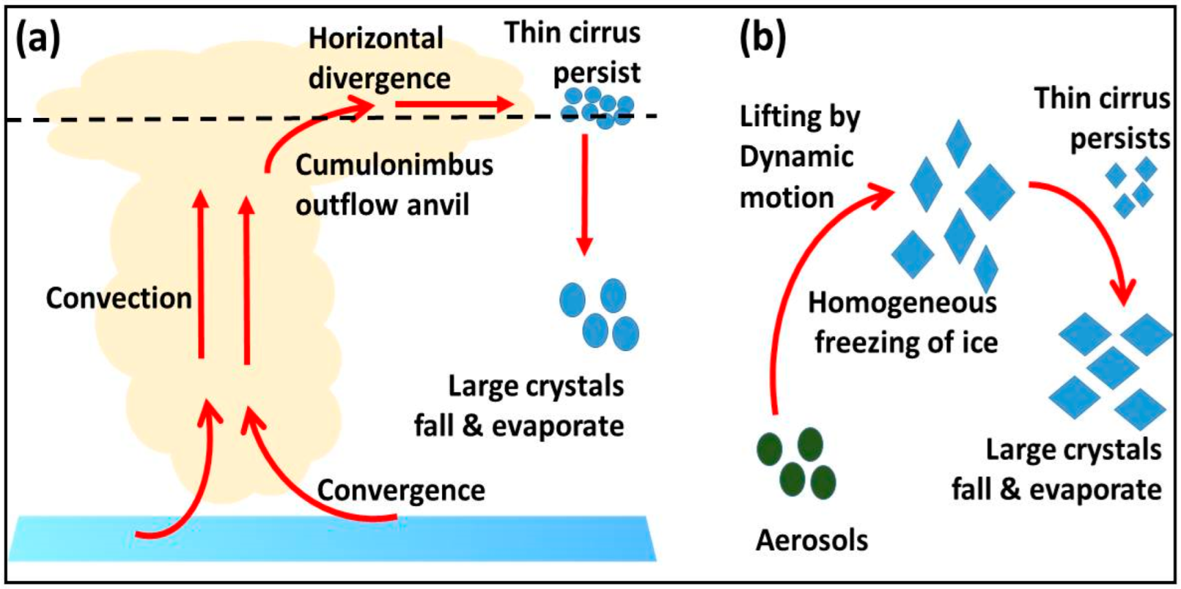
2.2. General Description of Cirrus Cloud Formation

Cirrus clouds are composed entirely of ice crystals instead of liquid moisture. They form at temperatures below −40 °C [18] and cover approximately 20–35% of the globe [19]. They affect Earth’s radiation allocation mainly by absorbing outgoing longwave radiation and by reflecting solar radiation. Two mechanisms (see Figure 1a,b) have been proposed for the formation of the cirrus clouds near the tropopause [20]. These mechanisms are (1) dissipation of optically thick cumulonimbus outflow anvils leaving behind an optically thin layer of small ice clouds (see Figure 1a), and (2) in situ nucleation of the ice crystals near the tropopause due to homogeneous freezing of high-altitude aerosols (see Figure 1b). In Figure 1a, the water and aerosols spread in the form of thick cirrus and cirrostratus clouds, generally below the tropopause level but seldom breaking through the tropopause into the lower stratosphere. At very low temperatures (~−70 °C) prevailing near the tropical tropopause, aerosols and water vapor coagulate or are frozen into ice-cloud particles. When the cirrus clouds melt, water vapor and aerosols separate out, leaving large relative humidity and high aerosol content in the upper troposphere, tropopause [20]. In Figure 1b, cirrus clouds form naturally in the upper troposphere when highly dilute aerosols cool and become supersaturated with respect to ice. Cloud particles freeze homogeneously when water vapor reaches ice supersaturations. This supersaturation required for ice nucleation may be generated by either slow, synoptic scale uplift or shear-driven turbulent mixing [20].

3. Data

3.1. CALIPSO

The CALIPSO satellite was launched on 28 April 2006 and is an integral part of NASA’s A-Train satellite constellation [21]. Its main objective is to study the role that clouds and aerosols play in regulating Earth’s weather, climate, and air quality. The main objectives of the CALIPSO are to (1) provide statistics on the vertical structure of clouds around the globe, (2) detect sub-visible clouds in the upper troposphere and Polar Stratospheric Clouds (PSC), and (3) provide statistics on the geographic and vertical distribution of aerosols and clouds around the globe. The primary instrument aboard CALIPSO is the Cloud-Aerosol Lidar with Orthogonal Polarization (CALIOP), a two-wavelength laser (532 nm and 1064 nm) operating at a pulse repetition rate of 20.16 Hz [22]. More information on the technical specifications of CALIPSO can be found in Winker et al. [23] and Winker et al. [24]. Furthermore, Winker et al. [24] give a detailed discussion on the algorithm that was developed to identify aerosol and cloud layers and to retrieve a variety of optical and microphysical properties.
Shikwambana and Sivakumar [25], Winker et al. [26], and Papagiannopoulos et al. [27], to name a few, have shown that Level 3 CALIPSO data products could be used for global studies. In this study, Level 3 cloud detection data were used for global retrievals of clouds for the period 2011–2016.

3.2. AIRS

AIRS (Atmospheric Infrared Sounder) on the EOS/Aqua satellite was launched in a polar orbit in May 2002. AIRS is a high spectral resolution spectrometer with 2378 IR channels between 3.74 and 4.61, 6.20–8.22, and 8.8–15.5 μm [28,29], which is essential for atmospheric temperature and relative humidity soundings. AIRS also has four visible and near-IR channels between 0.40 and 0.94 μm, which are mainly used for the detection of clouds in the IR Field of View (FOV). The AIRS retrieval algorithm has been developed and validated gradually with clear sky and clear/cloudy conditions over a non-frozen ocean and then the non-polar land and polar cases [30]. Retrievals yield cloud fraction, cloud top pressure and temperature, surface temperature, and vertical profiles of temperature and water vapor. The measurements’ vertical resolution and uncertainties are described by Aumann et al. [29]. In this study, cloud top temperature was used.

3.3. MERRA-2

The Modern-Era Retrospective analysis for Research and Applications, Version 2 (MERRA-2) is a reanalysis product generated by the NASA Global Modeling and Assimilation Office (GMAO) using the GEOS-5.12.4 system [31]. It replaces the original MERRA reanalysis [32] and includes updates to the AGCM [33] and the Global Statistical Interpolation atmospheric analysis scheme of Wu et al. [34]. MERRA-2 is produced using version 5.12.4 of the Goddard Earth Observing System Data Assimilation System (GEOS DAS). Gridded data are released at a 0.625° longitude × 0.5° latitude resolution on 72 sigma–pressure hybrid layers between the surface and 0.01 hPa. MERRA-2 assimilates bias-corrected aerosol optical depth (AOD) from the Moderate Resolution Imaging Spectroradiometer (MODIS) and the Advanced Very High-Resolution Radiometer instruments [35,36]. Buchard et al. [36] showed that the assimilated AOD observations do not constrain aerosol speciation, absorption properties, or aerosol vertical structure; the data assimilation system does produce diagnostics of these unconstrained quantities. They further showed that the accuracy of MERRA-2 aerosol diagnostics depends not only on the quality of AOD observed and the data assimilation algorithm but also on the quality of the background or forecast model. In this work, MERRA-2 is used to produce three-dimensional fields of cloud heights, total water vapor, and total precipitation land.

4. Results and Discussion

4.1. CALIPSO Cloud Occurrence

The daytime and night-time distribution of cloud height detection over latitude for 2011–2016 is shown in Figure 2. The color bar represents the heights of the clouds detected. The highest clouds for both daytime (left panels) and night-time (right panels) are found in the region of the Inter Tropical Convergence Zone (ITCZ), between 10° S and 10° N. The cloud height decreases gradually from the ITCZ due to the downward air streams in the Hadley cell. The lowest cloud heights are found towards both poles, which is due to the decrease in tropopause height [37]. Slight differences in cloud detections for daytime and night-time measurements are also observed. There is a greater occurrence of clouds during the night-time than during the daytime, especially in the lower altitudes (>2 km) in the region 40° S–80° S. One of the reasons for the greater cloud detection at night could be the formation of more low-level clouds. It is known that during the night, the heat stored during the daytime radiates back into space as infrared. The surface gets colder than the air, and that causes a thermal inversion. If there is enough moisture in the air, it may cause clouds to form in the lower altitudes. The yearly comparison of the latitudinal distribution of cloud detection from 2011 to 2016 further showed no major differences except in the 40° S–80° S region. In this region, cloud detection varied yearly, with the highest cloud detection observed in 2016. There are several factors such as surfacing heating, frontal, increase in the amount of water in the air, convergence, and turbulence that might have contributed to the increase in cloud formation in this region. Seasonal studies revealed a high dominance of clouds in the 70° S–80° S (Antarctic) region in the June–July–August (JJA) season (see Figure 3). The high cloud dominance could be attributed to the advection of the moist, maritime air caused by the cyclonic circulations over the Ross Sea and Amundsen Sea regions [38]. Moderate and low cloud detection is observed in the September–October–November (SON) and December–January–February (DJF) seasons, respectively, for the Antarctic region. A sudden decrease in the formation of clouds in the DJF season suggests that moisture transport and precipitation in the Antarctic region are primarily controlled by cyclonic activity rather than by air temperature [38]. On the other hand, Arctic clouds are dominant in the DJF and SON seasons and less dominant in the March–April–May (MAM) and JJA seasons. The formation of Arctic clouds is improved by enhanced turbulent heat fluxes from the surface and subsequent horizontal and vertical convergence of moisture and energy, suggesting a positive feedback effect on the surface temperature [39]. This might be one of the reasons for the dominance of Arctic clouds in the DJF and SON seasons.

4.2. Cloud Fraction Distribution for Low, Middle, and High Clouds

A 6-year global seasonal cloud fraction (CF) for low (left panel), middle (middle panel), and high (right panel) clouds is shown in Figure 4. The color bar represents the cloud fraction, which is the portion of each pixel that is covered by clouds. Throughout the seasons, low-level clouds are dominant (CF~0.8) in the polar regions. They are also dominant (CF~0.8) in the SON season in the Pacific and Atlantic Oceans and less dominant (CF > 0.01) over the land of the equatorial region. During this season, there is a release of large quantities of aerosols into the atmosphere as a result of biomass burning. Aerosols serve as CCN [40], which aid in cloud formation. Albrecht [41] further showed that an increase in aerosol concentrations tends to decrease the size of cloud droplets and makes the precipitation formation less efficient and increases cloud lifetime. Therefore, the dominance of clouds in the SON season in the equatorial region might be caused by aerosols from biomass burning. Middle-level clouds, on the other hand, are still observed in the polar regions but have a moderate cloud fraction of CF~0.5. The polar regions show the presence of middle-level clouds (CF~0.5) in every season, except for the JJA season, where the Arctic region shows a low CF~0.3. Middle clouds (with a low CF~0.2) are also observed every season over land and oceans in the equatorial region. High-level clouds with CF~0.8 are more distributed over the ITCZ region, which is correlated to deep convective clouds (DCC) [42]. DCC at high altitudes are able to penetrate the tropopause and play an important role in water vapor regulation in the lower stratosphere. The equatorial region of South America has a high CF value (~0.8) and a large latitude–longitude distribution in the SON, DJF, and MAM seasons. A lesser latitude–longitude distribution and a lower CF value (~0.6) are observed in the JJA season, which is the driest season. This could be attributed to a decline in rainfall as a consequence of climate change [43].

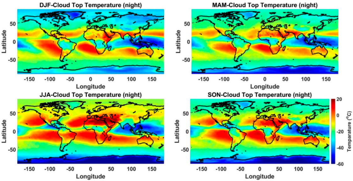
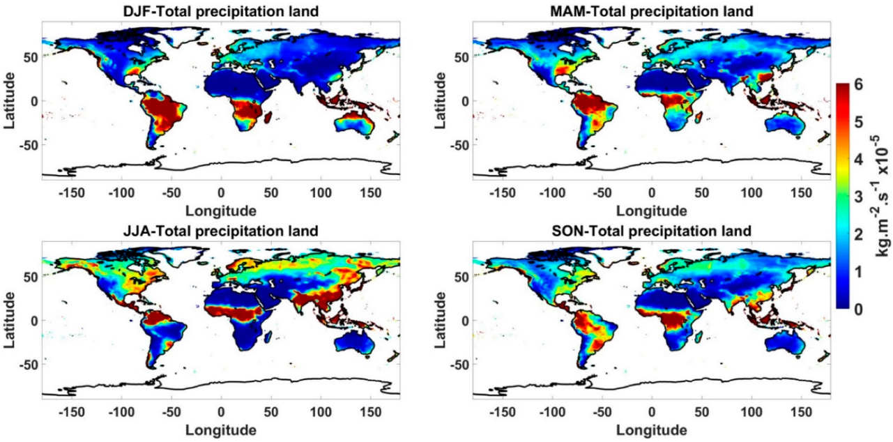
4.3. Cloud Top Temperature and Precipitation over Land

Temperatures inside a cloud can be important in modulating the cloud microphysics to produce precipitation [44]. The global seasonal averaged cloud top temperatures (CTT) color bar maps are shown in Figure 5. The coldest CTTs are mostly observed over land in the ITCZ and the polar regions, while the warmest CTTs are mostly observed in the mid-latitudes and over the oceans. JJA is the only season in South America that has CTT of 20 °C compared to CTT of ~−30 °C for the DJF, MAM, and SON seasons. This is also the season with the highest CTT (20 °C) in southern and northern Africa. This also correlates to low precipitation over land in those regions (see Figure 6). The color bar map in Figure 6 describes the rate at which precipitation falls to the ground. Generally, it is observed that regions with CTT greater than 0 °C experience less precipitation than regions with CTT less than 0 °C. As a way of example, in every season, central Africa has CTT (~−10 °C) and has consistent seasonal precipitation over the land of ~6 × 10⁻⁵ kg·m−2s−1. On the other hand, northern Africa has CTT (~20 °C) seasonally with seasonal precipitation over the land of ~>0.5 × 10⁻⁵ kg·m−2s−1. Legates and Illmott [45] inferred that two-thirds of the global precipitation falls in tropical regions of the earth between 30° N and 30° S. This was also observed in this work for the DJF, MAM, and SON seasons. However, in the JJA season, an increase in precipitation (between 3 − 6 × 10⁻⁵ kg·m−2s−1) was observed above 30° N latitude in the Eurasia region. Precipitation in this region increases due to convective precipitation and an increase in cyclone activities [46].

5. Conclusions

Clouds are important for global climate since they have a strong impact on solar and terrestrial radiation as well as on the formation of precipitation. The present paper uses various satellite and model data to study the global distribution of clouds for the period 2011–2016. The result from the study further shows that understanding clouds is critical for forecasting weather conditions, modeling the impacts of future climate change, and predicting the availability of water resources. The following are the important outcomes of the study.
(I)
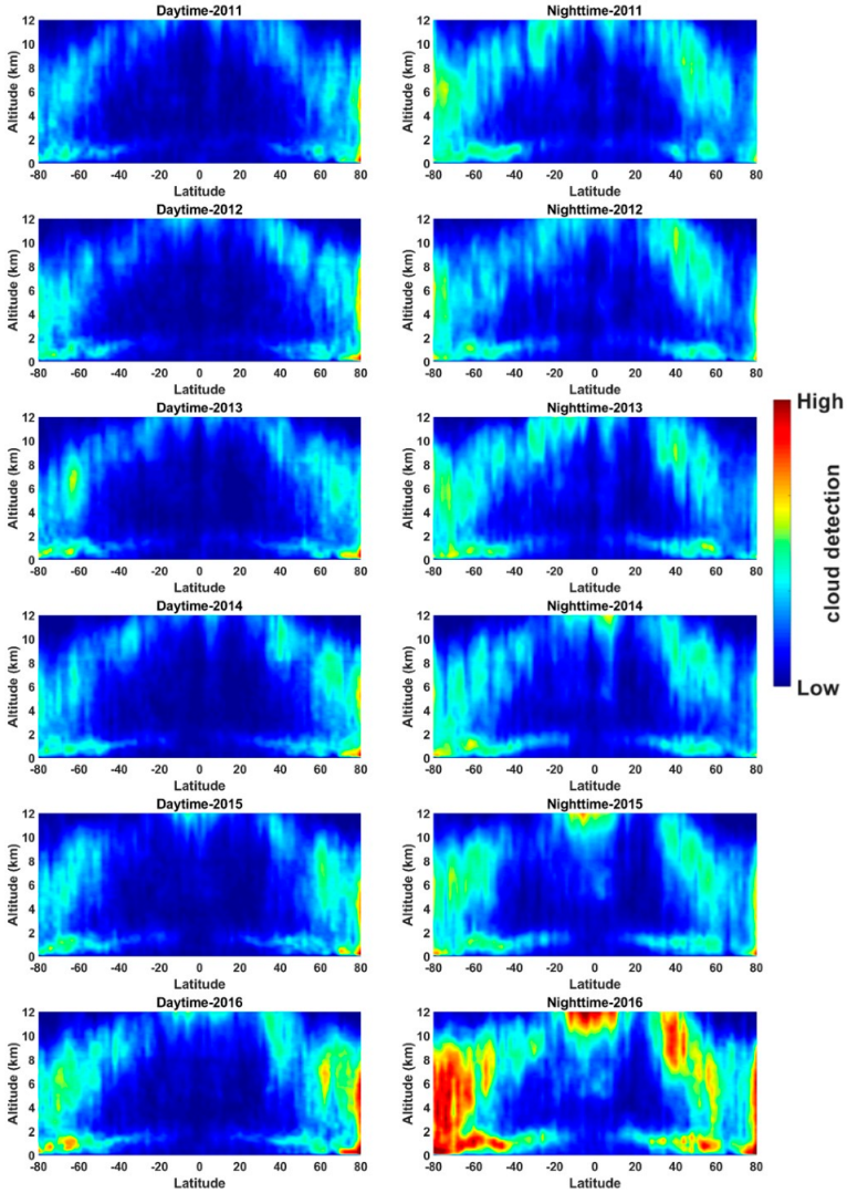
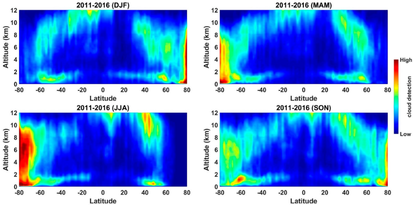
From CALIPSO observations, the highest clouds for both daytime and night-time are found in the ITCZ region. The lowest cloud heights are found towards the poles, which is due to the decrease in the tropopause height. There is a greater occurrence of clouds during the night-time, which is due to favorable conditions for the formation of low-level clouds. Seasonal studies revealed a high dominance of clouds in the 70° S–80° S (Antarctic) region in the JJA season and a high dominance of Arctic clouds in the DJF and SON seasons.
(II)
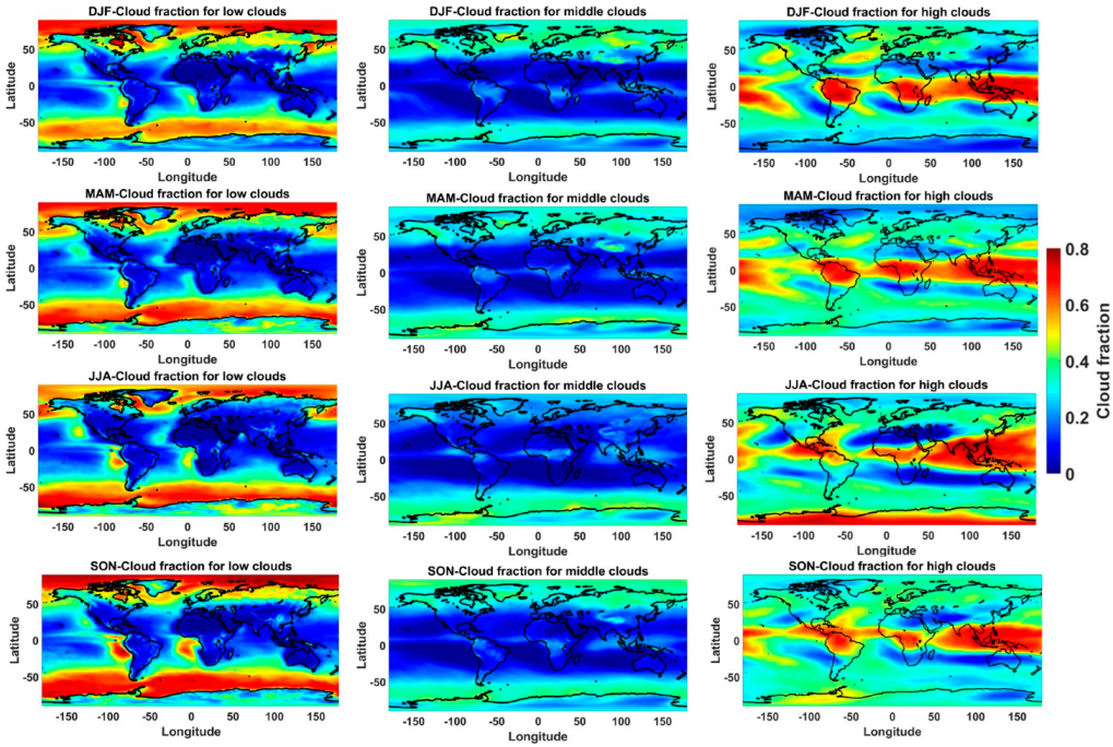
Using the MERRA-2 model data, it was observed that low-level clouds are dominant in the polar regions. Middle-level clouds are observed both in the polar regions and over land and oceans. High-level clouds are distributed over the ITCZ region. Most of the precipitation over land was observed between 30° N and 30° S in the DJF, MAM, and SON seasons. In the JJA season, precipitation was dominant above 30° N latitude in the Eurasia region.
(III)
The coldest CTTs are mostly observed over land in the ITCZ and the polar regions, while the warmest CTTs are mostly observed in the mid-latitudes and over the oceans. Regions with CTT greater than 0 °C experience less precipitation than regions with CTT less than 0 °C.

Funding

This research received no external funding. The APC was funded by the South African National Space Agency.

Institutional Review Board Statement

Not applicable.

Informed Consent Statement

Not applicable.

Data Availability Statement

The datasets generated during and/or analyzed during the current study are available from the corresponding author upon reasonable request. CALIPSO dataset can be accessed on https://search.earthdata.nasa.gov (accessed on 7 May 2022). MERRA-2 and AIRS dataset can be accessed on https://giovanni.gsfc.nasa.gov/giovanni.

Acknowledgments

We thank the Atmospheric Science Data Center at NASA Langley Research Center for archiving and hosting CALIPSO data. The MERRA-2 data used in this study have been provided by the Global Modeling and Assimilation Office (GMAO) at NASA Goddard Space Flight Center. We also like to thank the NASA Goddard Earth Sciences Data Information and Services Center (GESDISC) for the distribution of the AIRS data.

Conflicts of Interest

The author declares no conflict of interest.

References

  1. McFiggans, G.; Artaxo, P.; Baltensperger, U.; Coe, H.; Facchini, M.C.; Feingold, G.; Fuzzi, S.; Gysel, M.; Laaksonen, A.; Lohmann, U.; et al. The effect of physical and chemical aerosol properties on warm cloud droplet activation. Atmos. Chem. Phys. 2006, 6, 2593–2649. [Google Scholar] [CrossRef]
  2. Quante, M. The role of clouds in the climate system. J. Phys. IV 2004, 121, 61–86. [Google Scholar] [CrossRef]
  3. Zhou, C.; Zelinka, M.D.; Klein, S.A. Analyzing the dependence of global cloud feedback on the spatial pattern of sea surface temperature change with a Green’s function approach. J. Adv. Model. Earth Syst. 2017, 9, 2174–2189. [Google Scholar] [CrossRef]
  4. Qian, Y.; Long, C.N.; Wang, H.; Comstock, J.M.; McFarlane, S.A.; Xie, S. Evaluation of cloud fraction and its radiative effect simulated by IPCC AR4 global models against ARM surface observations. Atmos. Chem. Phys. 2012, 12, 1785–1810. [Google Scholar] [CrossRef]
  5. Kassianov, E.; Long, C.N.; Ovtchinnikov, M. Cloud Sky Cover versus Cloud Fraction: Whole-Sky Simulations and Observations. J. Appl. Meteorol. 2005, 44, 86–98. [Google Scholar] [CrossRef]
  6. Chen, L.; Yan, G.; Wang, T.; Ren, H.; Calbó, J.; Zhao, J.; McKenzie, R. Estimation of surface shortwave radiation components under all sky conditions: Modeling and sensitivity analysis. Remote Sens. Environ. 2012, 123, 457–469. [Google Scholar] [CrossRef]
  7. Randall, D.; Coakley, J., Jr.; Fairall, C.; Kropfli, R.; Lenschow, D. Outlook for research on subtropical marine stratiform clouds. Bull. Am. Meteorol. Soc. 1984, 65, 1290–1301. [Google Scholar] [CrossRef]
  8. Long, C.N.; Sabburg, J.; Calbó, J.; Pagès, D. Retrieving cloud characteristics from ground-based daytime color all-sky images. J. Atmos. Ocean. Technol. 2006, 23, 633–652. [Google Scholar] [CrossRef]
  9. Stubenrauch, C.J.; Rossow, W.B.; Kinne, S.; Ackerman, S.; Cesana, G.; Chepfer, H.; Di Girolamo, L.; Getzewich, B.; Guignard, A.; Heidinger, A.; et al. Assessment of Global Cloud Datasets from Satellites: Project and Database Initiated by the GEWEX Radiation Panel. Bull. Am. Meteorol. Soc. 2013, 94, 1031–1049. [Google Scholar] [CrossRef]
  10. Kim, S.-W.; Chung, E.-S.; Yoon, S.-C.; Sohn, B.-J.; Sugimoto, N. Intercomparisons of cloud-top and cloud-base heights from ground-based Lidar, CloudSat and CALIPSO measurements. Int. J. Remote Sens. 2011, 32, 1179–1197. [Google Scholar] [CrossRef]
  11. Hagihara, Y.; Okamoto, H.; Yoshida, R. Development of a combined CloudSat-CALIPSO cloud mask to show global cloud distribution. J. Geophys. Res. 2010, 115, D00H33. [Google Scholar] [CrossRef]
  12. Sassen, K.; Wang, Z.; Liu, D. Global distribution of cirrus clouds from CloudSat/Cloud-Aerosol Lidar and Infrared Pathfinder Satellite Observations (CALIPSO) measurements. J. Geophys. Res. 2008, 113, D00A12. [Google Scholar] [CrossRef]
  13. Sassen, K.; Wang, Z.; Liu, D. Cirrus clouds and deep convection in the tropics: Insights from CALIPSO and CloudSat. J. Geophys. Res. 2009, 114, D00H06. [Google Scholar] [CrossRef]
  14. Noel, V.; Hertzog, A.; Chepfer, H.; Winker, D.M. Polar stratospheric clouds over Antarctica from the CALIPSO spaceborne lidar. J. Geophys. Res. 2008, 113, D02205. [Google Scholar] [CrossRef]
  15. Fu, Y.; Chen, Y.; Li, R.; Qin, F.; Xian, T.; Yu, L.; Zhang, A.; Liu, G.; Zhang, X. Lateral Boundary of Cirrus Cloud from CALIPSO Observations. Sci. Rep. 2017, 7, 14221. [Google Scholar] [CrossRef]
  16. Pitts, M.C.; Poole, L.R.; Gonzalez, R. Polar stratospheric cloud climatology based on CALIPSO spaceborne lidar measurements from 2006 to 2017. Atmos. Chem. Phys. 2018, 18, 10881–10913. [Google Scholar] [CrossRef]
  17. Naeger, A.R.; Christopher, S.A.; Ferrare, R.; Liu, Z. A New Technique Using Infrared Satellite Measurements to Improve the Accuracy of the CALIPSO Cloud-Aerosol Discrimination Method. IEEE Trans. Geosci. Remote Sens. 2013, 51, 642–653. [Google Scholar] [CrossRef]
  18. Lynch, D.K.; Sassen, K.; Starr, D.; Stephens, G. Cirrus; Oxford University Press: New York, NY, USA, 2002. [Google Scholar]
  19. Liou, K.N. Influence of cirrus clouds on weather and climate processes: A global perspective. Mon. Weather Rev. 1986, 114, 1167–1199. [Google Scholar] [CrossRef]
  20. Veerabuthiran, S. High-altitude cirrus clouds and climate. Resonance 2004, 9, 23–32. [Google Scholar] [CrossRef]
  21. Stephens, G.L.; Vane, D.G.; Boain, R.J.; Mace, G.G.; Sassen, K.; Wang, Z.; Illingworth, A.J.; CloudSat Science Team. The CloudSat mission and the A-Train: A new dimension of space-based observations of clouds and precipitation. Bull. Am. Meteorol. Soc. 2002, 83, 1771–1790. [Google Scholar] [CrossRef] [Green Version]
  22. Hunt, W.H.; Winker, D.M.; Vaughan, M.A.; Powell, K.A.; Lucker, P.L.; Weimer, C. CALIPSO Lidar Description and Performance Assessment. J. Atmos. Ocean. Technol. 2009, 26, 1214–1228. [Google Scholar] [CrossRef]
  23. Winker, D.M.; Pelon, J.; McCormick, M.P. The CALIPSO mission: Spaceborne lidar for observation of aerosols and clouds. In Proceedings of the SPIE 4893, Lidar Remote Sensing for Industry and Environment Monitoring III, Hangzhou, China, 8 May 2003. [Google Scholar]
  24. Winker, D.M.; Vaughan, M.A.; Omar, A.; Hu, Y.; Powell, K.A. Overview of the CALIPSO Mission and CALIOP Data Processing Algorithms. J. Atmos. Ocean. Technol. 2009, 26, 2310–2323. [Google Scholar] [CrossRef]
  25. Shikwambana, L.; Sivakumar, V. Global distribution of aerosol optical depth in 2015 using CALIPSO level 3 data. J. Atmos. Sol.-Terr. Phys. 2018, 173, 150–159. [Google Scholar] [CrossRef]
  26. Winker, D.M.; Tackett, J.L.; Getzewich, B.J.; Liu, Z.; Vaughan, M.A.; Rogers, R.R. The global 3-D distribution of tropospheric aerosols as characterized by CALIOP. Atmos. Chem. Phys. 2013, 13, 3345–3361. [Google Scholar] [CrossRef]
  27. Papagiannopoulos, N.; Mona, L.; Alados-Arboledas, L.; Amiridis, V.; Baars, H.; Binietoglou, I.; Bortoli, D.; D’Amico, G.; Giunta, A.; Guerrero-Rascado, J.L.; et al. CALIPSO climatological products: Evaluation and suggestions from EARLINET. Atmos. Chem. Phys. 2016, 16, 2341–2357. [Google Scholar] [CrossRef]
  28. Morse, P.G.; Bates, J.C.; Miller, C.R.; Chahine, M.T.; O’Callaghan, F.; Aumann, H.H.; Karnik, A.R. Development and test of the Atmospheric Infrared Sounder (AIRS) for the NASA Earth Observing System (EOS). In Proceedings of the SPIE 3870, Sensors, Systems, and Next-Generation Satellites III, Florence, Italy, 28 December 1999. [Google Scholar]
  29. Aumann, H.H.; Chahine, M.T.; Gautier, C.; Goldberg, M.D.; Kalnay, E.; McMillin, L.M.; Revercomb, H.; Rosenkranz, P.W.; Smith, W.L.; Staelin, D.H.; et al. AIRS/AMSU/HSB on the Aqua mission: Design, science objectives, data products, and processing systems. IEEE Trans. Geosci. Remote Sens. 2003, 41, 253–264. [Google Scholar] [CrossRef]
  30. Tobin, D.C.; Revercomb, H.; Knuteson, R.O.; Lesht, B.M.; Strow, L.L.; Hannon, S.E.; Feltz, W.F.; Moy, L.A.; Fetzer, E.J.; Cress, T.S. Atmospheric radiation measurement site atmospheric state best estimates for atmospheric infrared sounder temperature and water vapor retrieval validation. J. Geophys. Res. 2006, 111, D09S14. [Google Scholar] [CrossRef]
  31. Bosilovich, M.G.; Santha, A.; Coy, L.; Cullather, R.; Draper, C.; Geloro, R.; Kovach, R.; Liu, Q.; Molod, A.; Norris, P.; et al. MERRA-2: Initial Evaluation of the Climate; NASA/TM-2015-104606, Technical Report Series on Global Modeling and Data Assimilation; NASA: Greenbelt, MD, USA, 2015; Volume 43.
  32. Rienecker, M.M.; Suarez, M.J.; Gelaro, R.; Todling, R.; Bacmeister, J.; Liu, E.; Bosilovich, M.G.; Schubert, S.D.; Takacs, L.; Kim, G.; et al. MERRA: NASA’s Modern-Era Retrospective Analysis for Research and Applications. J. Clim. 2011, 24, 3624–3648. [Google Scholar] [CrossRef]
  33. Molod, A.; Takacs, L.; Suarez, M.; Bacmeister, J. Development of the GEOS-5 atmospheric general circulation model: Evolution from MERRA to MERRA-2. Geosci. Model Dev. 2015, 8, 1339–1356. [Google Scholar] [CrossRef]
  34. Wu, W.-S.; Purser, R.J.; Parrish, D.F. Three-dimensional variational analysis with spatially inhomogeneous covariances. Mon. Weather Rev. 2002, 130, 2905–2916. [Google Scholar] [CrossRef]
  35. Buchard, V.; Randles, C.A.; da Silva, A.M.; Darmenov, A.; Colarco, P.R.; Govindaraju, R.; Ferrare, R.; Hair, J.; Beyersdorf, A.J.; Ziemba, L.D.; et al. The MERRA-2 Aerosol Reanalysis, 1980 Onward. Part II: Evaluation and Case Studies. J. Clim. 2017, 30, 6851–6872. [Google Scholar] [CrossRef]
  36. Randles, C.A.; da Silva, A.M.; Buchard, V.; Colarco, P.R.; Darmenov, A.; Govindaraju, R.; Smirnov, A.; Holben, B.; Ferrare, R.; Hair, J.; et al. The MERRA-2 Aerosol Reanalysis, 1980 Onward. Part I: System Description and Data Assimilation Evaluation. J. Clim. 2017, 30, 6823–6850. [Google Scholar] [CrossRef]
  37. Kokhanovsky, A.; Vountas, M.; Burrows, J.P. Global Distribution of Cloud Top Height as Retrieved from SCIAMACHY Onboard ENVISAT Spaceborne Observations. Remote Sens. 2011, 3, 836–844. [Google Scholar] [CrossRef]
  38. Nicolas, J.P.; Bromwich, D.H. Climate of West Antarctica and influence of marine air intrusions. J. Clim. 2011, 24, 49–67. [Google Scholar] [CrossRef]
  39. Curry, J.A.; Rossow, W.B.; Randall, D.; Schramm, J.L. Overview of Arctic cloud and radiation characteristics. J. Clim. 1996, 9, 1731–1764. [Google Scholar] [CrossRef]
  40. Warner, J.; Twomey, S. The production of cloud nuclei by cane fires and the effect on cloud droplet concentration. J. Atmos. Sci. 1967, 24, 704–706. [Google Scholar] [CrossRef]
  41. Albrecht, B.A. Aerosols, cloud microphysics and fractional cloudiness. Science 1989, 245, 1227–1230. [Google Scholar] [CrossRef]
  42. Schiffer, R.A.; Rossow, W.B. The International Satellite Cloud Climatology Project (ISCCP): The First Project of the World Climate Research Programme. Bull. Am. Meteorol. Soc. 1983, 64, 779–784. [Google Scholar] [CrossRef]
  43. Malhi, Y.; Roberts, T.J.; Betts, R.A.; Killeen, T.J.; Li, W.; Nobre, C.A. Climate change, deforestation and the fate of the Amazon. Science 2008, 319, 169–172. [Google Scholar] [CrossRef]
  44. Hanna, J.W.; Schultz, D.M.; Irving, A.R. Cloud-Top Temperatures for Precipitating Winter Clouds. J. Appl. Meteor. Climatol. 2008, 47, 351–359. [Google Scholar] [CrossRef] [Green Version]
  45. Legates, D.R.; Willmott, C.J. Mean seasonal and spatial variability in gauge-corrected, global precipitation. Int. J. Climatol. 1990, 10, 111–127. [Google Scholar] [CrossRef]
  46. Serreze, M.C.; Barrett, A.P.; Lo, F. Northern High-Latitude Precipitation as Depicted by Atmospheric Reanalyses and Satellite Retrievals. Mon. Weather Rev. 2005, 133, 3407–3430. [Google Scholar] [CrossRef]
Figure 1. Schematic illustration of the formation of cirrus clouds by two mechanisms. (a) Dissipation of cumulonimbus outflow anvils and (b) in situ nucleation.
Atmosphere 13 01514 g001
Figure 2. Daytime (left panels) and night-time (right panels) latitudinal distribution of cloud heights for the period of 2011–2016 using CALIPSO.
Atmosphere 13 01514 g002
Figure 3. Seasonal averaged (2011–2016) latitudinal distribution cloud detection using CALIPSO.
Atmosphere 13 01514 g003
Figure 4. Seasonal averaged distribution of cloud fraction for low (left panel), middle (middle panel), and high (right panel) clouds using the MERRA-2 model data.
Atmosphere 13 01514 g004
Figure 5. S Seasonal averaged AIRS cloud top temperature for the period 2011–2016.
Atmosphere 13 01514 g005
Figure 6. Seasonal averaged total precipitation land for the period 2011–2016.
Atmosphere 13 01514 g006
Publisher’s Note: MDPI stays neutral with regard to jurisdictional claims in published maps and institutional affiliations.

