Article

Propagation of a Meteotsunami from the Yellow Sea to the Korea Strait in April 2019

1
Jeju Marine Research Center, Korea Institute of Ocean Science & Technology, Jeju 63349, Korea
2
Department of Oceanography, Chonnam National University, Gwangju 61186, Korea
*
Author to whom correspondence should be addressed.
Atmosphere 2021, 12(8), 1083; https://doi.org/10.3390/atmos12081083
Submission received: 25 June 2021 / Revised: 13 August 2021 / Accepted: 20 August 2021 / Published: 23 August 2021

Abstract

:
A meteotsunami with a wave height of 0.1–0.9 m and a period of 60 min was observed at tide gauges along the Korea Strait on 7 April 2019, while a train of two to four atmospheric pressure disturbances with disturbance heights of 1.5–3.9 hPa moved eastward from the Yellow Sea to the Korea Strait. Analysis of observational data indicated that isobar lines of the atmospheric pressure disturbances had angles of 75–83° counterclockwise due east and propagated with a velocity of 26.5–31.0 m/s. The generation and propagation process of the meteotsunami was investigated using the Regional Ocean Modeling System. The long ocean waves were amplified due to Proudman resonance in the southwestern Yellow Sea, where the water is deeper than 75 m; here, the long ocean waves were refracted toward the coast on the shallow coastal region of the northern Korea Strait. Refraction and reflection by offshore islands significantly affect the wave heights at the coast. To investigate the effects of an eastward-moving velocity and angle of atmospheric pressure disturbance on the height of a long ocean wave, sensitivity simulations were performed. This result will be useful for the real-time prediction system of meteotsunamis in the Korea Strait.

1. Introduction

A meteotsunami, a tsunami-like long ocean wave, is generated by atmospheric pressure disturbances, atmospheric gravity waves, and squalls propagating over the ocean surface [1,2]. Long ocean waves are induced in the process of rapid change and restoration of sea level by this atmospheric forcing. The long ocean waves are amplified by Proudman [3], Greenspan [4], shelf, and harbor resonances depending on the region, and it has been suggested that Proudman resonance is the main cause of meteotsunami amplification worldwide [5]. Proudman resonance occurs when the propagation speed ( C ) of the generated ocean wave is close to the movement speed ( U ) of pressure perturbations [1,6,7,8,9]:
C = g H
where g is gravitational acceleration and H is the water depth. When the Froude number ( Fr = U / C ) is close to 1.0, a strong amplification of the long ocean wave occurs by absorbing the energy of moving atmospheric pressure disturbances (i.e., Proudman resonance) [10]. The long ocean waves propagating along the coast are also amplified due to Greenspan resonance; the amplification depends on the wave period and bottom topographic slope [4]. However, these external resonances alone do not make a destructive meteotsunami. The long ocean waves generated by external resonance are amplified as they propagate into semienclosed bays, and water depth becomes shallower; the amplification strength of the waves varies depending on the size, shape, and depth of the water body. The long ocean is further amplified due to harbor resonance in a long narrow bay when the period of the long ocean wave is close to the natural resonant periods of a bay [11,12,13,14]. If these long ocean waves reach the shore during high tide, even in calm weather, they can cause coastal flooding by high sea level oscillations and become a devastating natural disaster [15,16].
The causes and damage conditions of meteotsunami events known around the world are summarized in [2]. There have been several reports of disasters caused by meteotsunamis in the Yellow Sea and East China Sea [2,17]. On 31 March 1979, a meteotsunami occurred in Nagasaki Bay, Japan, with a maximum sea level anomaly of 4.8 m [1,18]. Meteotsunamis induced a strong current, making severe damage to cargo vessels and fishing boats by tearing their mooring lines in Nagasaki Bay. Due to the meteotsunami on 25 February 2009, with a maximum wave height of 2.9 m, 30 vessels were capsized and damaged in western Kyushu, and eight residences were inundated below floor level [19]. A meteotsunami caused by a pressure disturbance moving southeast from the eastern Yellow Sea resulted in the death of three people along the west coast of Korea on 31 March 2007 [15,20]. The meteotsunami overlapped with high tide, causing severe inundation along the coast and capsizing more than 90 vessels along the west coast of Korea [15]. Recently, a real-time pressure disturbance monitoring system was developed for the prevention of meteotsunami disasters based on the available atmospheric pressure data from 89 automatic weather stations (AWS) along the Korean coastline [21].
There were 42 events of sea level oscillations due to the arrival of long ocean waves with wave heights higher than 40 cm in Jinhae-Masan Bay (128.4–128.8° E, 34.9–35.3° N) in the Korea Strait from 2013 to 2017, and the periods of the long ocean waves were 48–125 min [22]. The abnormal sea level rise observed at MS in the past resulted in wave heights of up to 80 cm, and when it overlaps with high tides, flooding of low-lying regions may occur [22]. On 7 April 2019, long ocean waves with a wave height of 0.9 m arrived at MS in the Korea Strait, and there was a flood threat due to the high sea level oscillations in Jinhae-Masan Bay. However, there is no explanation for the generation mechanism of the long ocean waves that were observed in the Korea Strait on 7 April 2019. In this study, the generation mechanism and propagation process of the long ocean waves that were observed on 7 April 2019, in the Korea Strait were investigated using observational data and numerical simulations.
Observational data and two-dimensional numerical simulations are introduced in Section 2. In Section 3, the time series of the observed atmospheric pressure and sea level data in the Korea Strait are analyzed, and two-dimensional numerical simulations are performed to determine the generation and propagation processes of the long ocean waves that occurred on 7 April 2019. In Section 4, possible amplification mechanisms for long ocean waves in the Korea Strait are discussed, the role of offshore islands on the refraction and reflection of long ocean waves toward Jinhae-Masan Bay is examined, the resonance effects due to local features are explained, and numerical model simulations are performed to find the angle and speed at which Proudman resonance can occur most effectively. Finally, conclusions are drawn in Section 5.

2. Materials and Methods

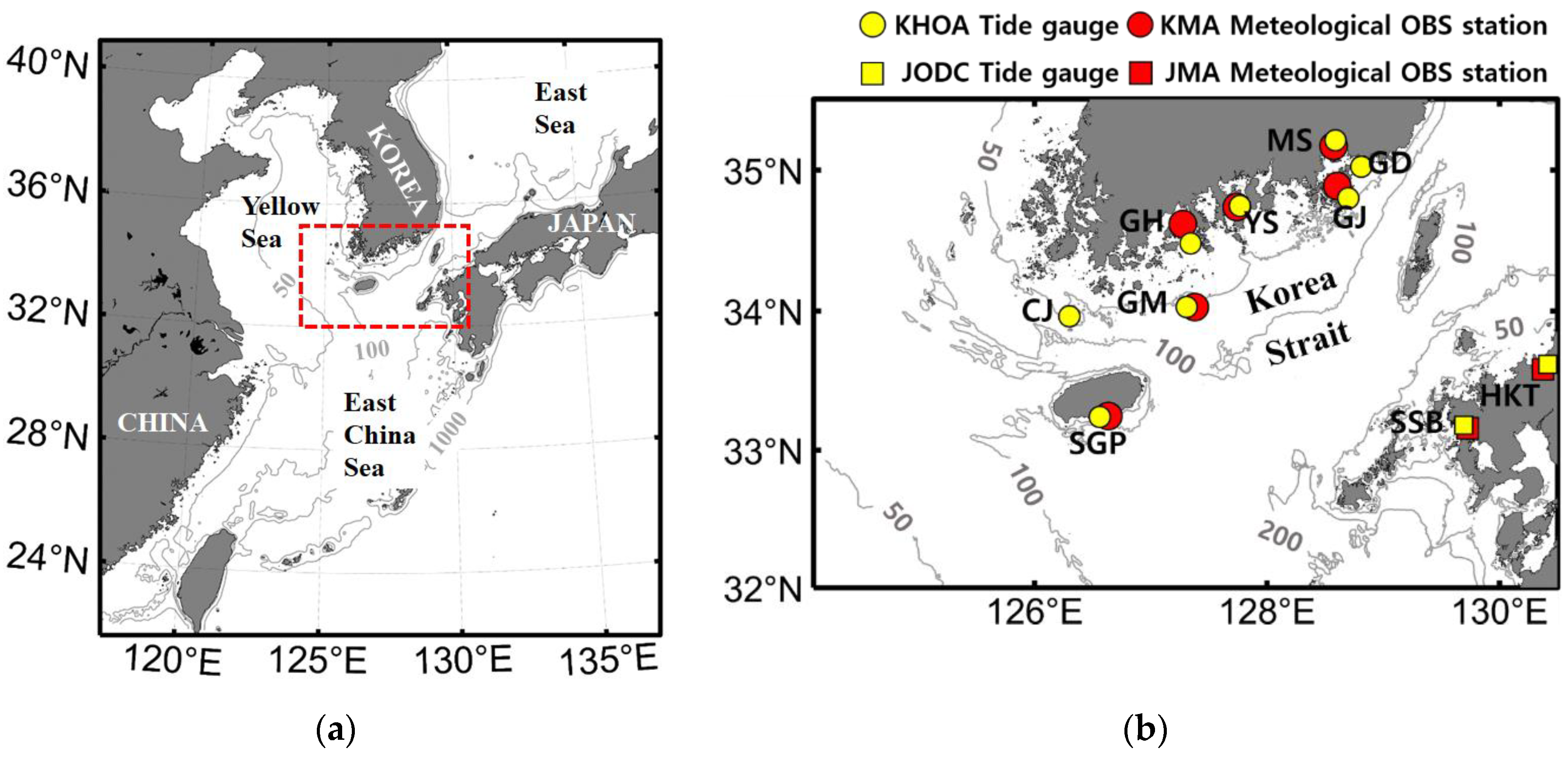
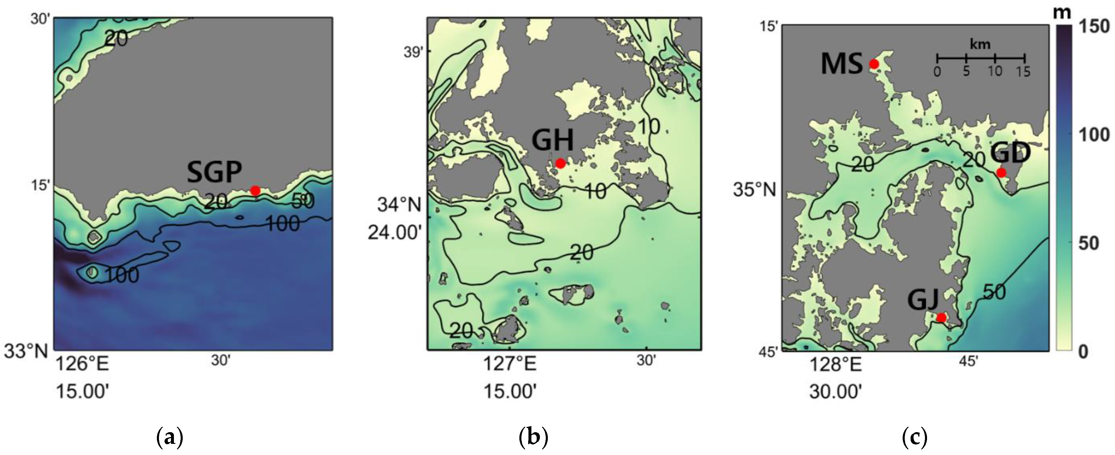
2.1. Observational Data

To understand the generation and propagation of meteotsunamis in the Korea Strait, the time series of atmospheric pressure and sea level data observed at meteorological stations and tide gauge stations were used. Data were obtained from a total of 10 stations: CJ, SGP, GM, GH, YS, GJ, GD, MS, SSB, and HKT (Figure 1b). In this study, atmospheric pressure and sea level data from 7 to 8 April 2019 were analyzed, and local standard time (UTC + 9 h) was used. Atmospheric pressure data were supplied by the Korea Meteorological Administration (KMA) and Japan Meteorological Agency (JMA), and the data intervals were 1 and 10 min, respectively. Sea level data were provided by the Korea Hydrographic and Oceanographic Agency (KHOA) and Japan Oceanographic Data Center (JODC), and the data intervals were 1 and 10 min, respectively. Atmospheric pressure data were obtained with automatic weather station (AWS) and automated surface observing systems (ASOS), and sea level was measured using float-type tide gauges.
By analyzing the time series of atmospheric pressure and sea level data in the Korea Strait, the movement direction and speed of atmospheric pressure disturbances and long ocean waves (meteotsunami) were estimated. The horizontal movement of squall lines was traced from the rainfall intensity radar images provided by the KMA. A high-pass filter with a cutoff period of 180 min was used to remove tide signals in the sea level data and low-frequency variability in the atmospheric pressure data. Wavelet analysis was performed on the time series of atmospheric pressure and sea level data to find peak energy periods and event durations in the data.

2.2. Numerical Model Simulation

To reproduce the generation of a meteotsunami in the Korea Strait and analyze the propagation process, two-dimensional numerical modeling experiments were conducted using the Regional Ocean Modeling System (ROMS) [23,24]. The model domain encompassed the shelf sea region of 32.0–35.3° N, 122.4–129.6° E, including the Korea Strait, which is located between the Yellow Sea, East China Sea, and East Sea (Figure 1b). The horizontal grid spacing of the model was approximately 300 m. The bottom topography data were obtained from the Korbathy 30s bathymetry dataset [25], and the minimum water depth was 0.1 m.
The numerical model was forced only by a train of moving atmospheric pressure disturbances. The movement direction, speed, angle, and wave period of the atmospheric pressure forcing were estimated based on the analysis results of the KMA and JMA observation data. The initial temperature, salinity, and sea level in the numerical model were uniform, set as 15 °C, 30 psu, and 0 m, respectively. Wind forcing was not considered because the wind speed at the time of the meteotsunami event was weak (<3 m/s). For the open boundaries of the numerical model, Chapman [26] and Flather [27] conditions were used for sea level and velocity, respectively. The time step of the model was 3 s, and the simulation was performed for 24 h. The numerical simulations in this study were performed with an analytical forcing and initial condition. In order to quantify the role of offshore islands on the refraction and reflection of long ocean waves and the amplitude of sea level oscillations at the coastal tide gauge stations, an additional numerical experiment was performed without the offshore islands. To find the critical movement speed and angle of atmospheric pressure disturbances that are optimal to induce the largest sea level oscillations by Proudman resonance in the Korea Strait, a range of movement speeds of 20–40 m/s and angles of 60–120° were applied in sensitivity experiments.

3. Results

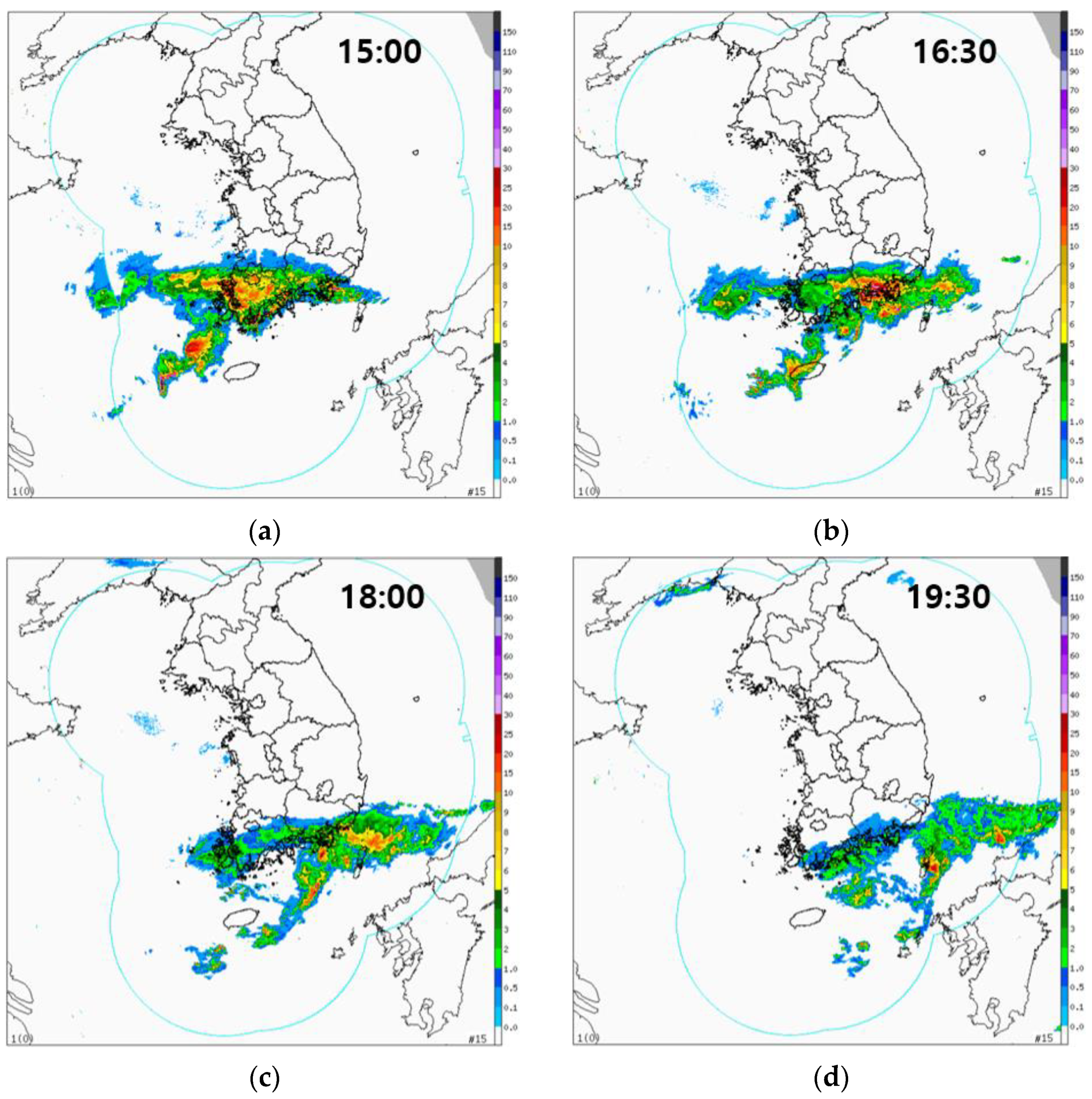
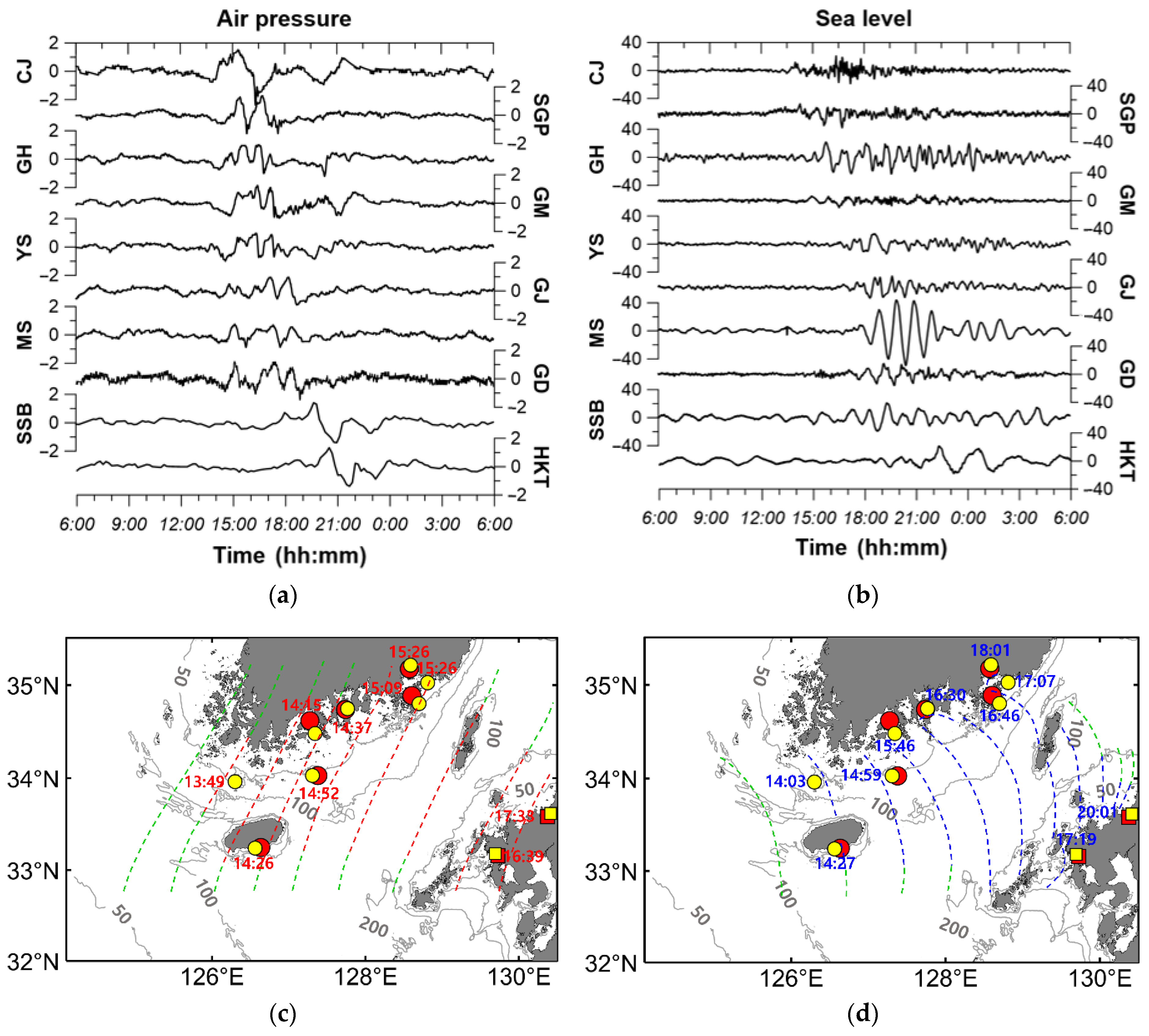
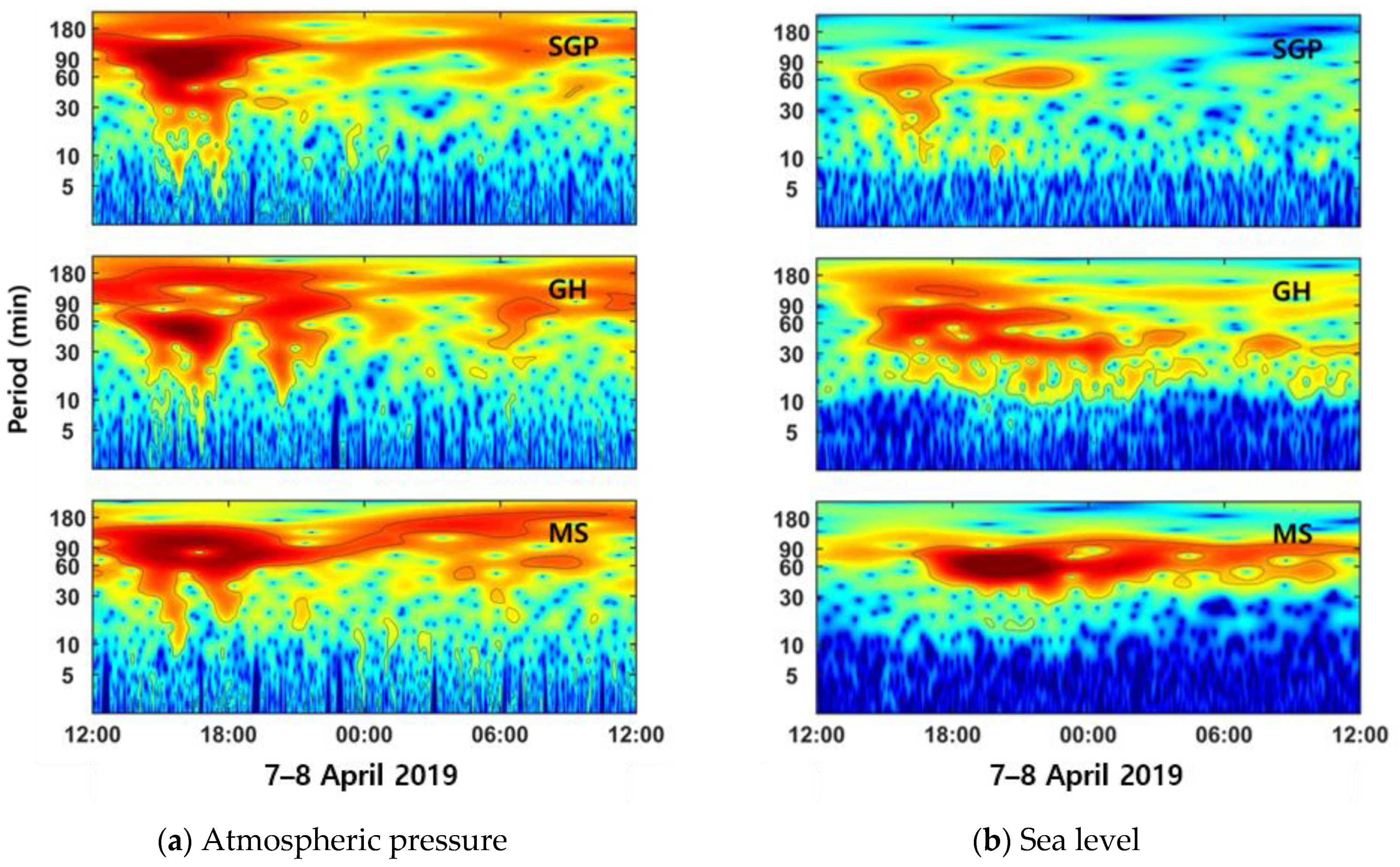
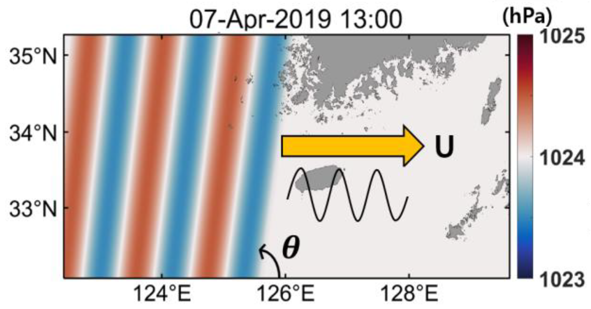
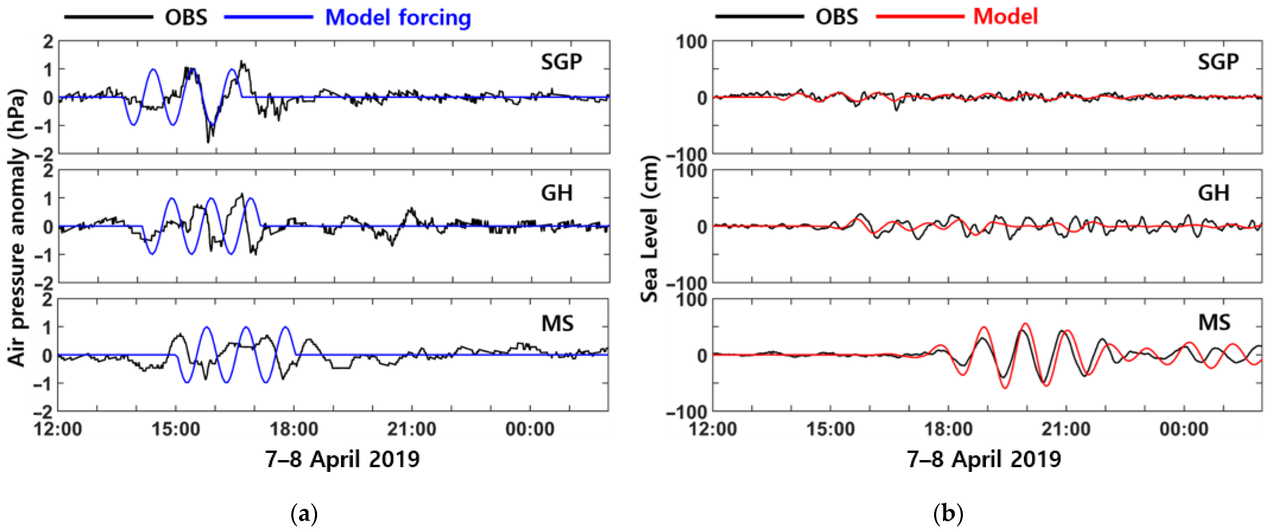
3.1. Atmospheric and Ocean Observation

On 7 April 2019, convective rain clouds were observed moving from west to east in the Korea Strait (Figure 2). A zonal band of rain clouds moved eastward along the northern coast of the Korea Strait, and a southern branch of rain clouds to the west of Jeju Island headed toward the island at 15:00 on 7 April. Atmospheric pressure disturbances propagated ahead of the southern branch of rain clouds (Figure 2 and Figure 3). It could be observed that the atmospheric pressure jumps were tilted spatially, and the titling angle was approximately 80° counterclockwise due east (Figure 3). The trains of atmospheric pressure disturbances arrived at CJ at 13:49 on 7 April, and moved over SGP, GM, and MS at 14:29, 14:50, and 15:46, respectively (Figure 3a,c and Table 1). The arrival times of the atmospheric pressure disturbances were defined as the time of the lowest elevation point of the first anomaly peak. The movement angle and time were spatially inferred using the arrival time of the atmospheric pressure disturbances at each station (red dashed line in Figure 3c). The line of atmospheric pressure jumps was inclined at approximately 75–83° counterclockwise due east in the Korea Strait. The angle gradually increased as it moved from west to east, because the eastward-moving speed of atmospheric pressure disturbances was faster in the south than the north from 13:30 to 14:30 on 7 April (Figure 2 and Figure 3c). Once the disturbances passed the GH and GM stations, the angle was maintained at 75–80°. The speeds of the atmospheric pressure disturbances were calculated using differences in the arrival times and distances between each station in the east–west direction based on the observed data. The speeds of the atmospheric pressure disturbances along the northern coastal stations (GH–GD), central stations (CJ–GM), and southern stations (SGP–HKT) of the Korea Strait were approximately 31.0, 26.5, and 30.4 m/s, respectively (Figure 3c and Table 1). The height of atmospheric pressure disturbances from trough to crest was approximately 1.5–3.9 hPa (Table 1). Atmospheric pressure disturbances consisting of two to four waves moved eastward along the Korea Strait (Figure 3a).
During the passage of atmospheric pressure disturbances, the sea level oscillations were observed along the Korea Strait (Figure 3b). The sea level oscillation started at 13:59 at CJ and arrived at GH and MS at 15:07 and 17:48, and the maximum wave heights from trough to crest were 38.1, 42.5, and 91.9 cm, respectively (Figure 3b and Table 2). The highest wave height was observed at MS. The tidal range of sea level at the MS tide observation station is from 120 cm during the neap tide to 240 cm during the spring tide. The tidal range at MS was 188 cm on 7 April 2019. The start time of sea level oscillation was defined as the time of the highest point of the first peak in sea level variations. The wave height at the offshore stations in the western Korea Strait, such as CJ, SGP, and GM, was relatively small, from 16.3 to 38.1 cm, and the sea level oscillations started 8–15 min after the passage of an atmospheric pressure disturbance. However, at the GH, YS, GJ, MS, GD, SSB, and HKT stations, located on the coast or in a bay of the eastern Korea Strait, the wave height in sea level oscillations was relatively large, but the sea level oscillations started approximately 40–115 min after the passage of atmospheric pressure disturbances. The spatial propagation patterns of the waves were inferred using the arrival times of the long ocean waves at each station (blue dashed lines in Figure 3d). Propagation analysis of the observed sea level data revealed that the long ocean waves propagate from the southwest to the northeast of the Korea Strait.
To determine the dominant periods and duration of atmospheric pressure and the sea level oscillations, wavelet spectrum analysis was performed on the time series of atmospheric pressure and sea level data at SGP, GH, and MS. The SGP, GH, and MS stations are located in the southwest, north, and northeast of the Korea Strait, respectively. The dominant periods of atmospheric pressure fluctuations were 40–115 min and lasted for 7–19 h (Figure 4a). The sea level oscillations at SGP and GH had relatively large energy in the periods of 10–90 and 10–160 min and lasted for approximately 7 and 12 h, respectively. The sea level oscillations at MS had relatively distinct periods of 35–90 min. The sea level oscillation was relatively strong for the first 5 h, and it lasted approximately 14 h. The durations of sea level oscillation were longer at the GH and MS stations, which are located in shallow and coastal regions, than at the SGP station, which is in an offshore area.

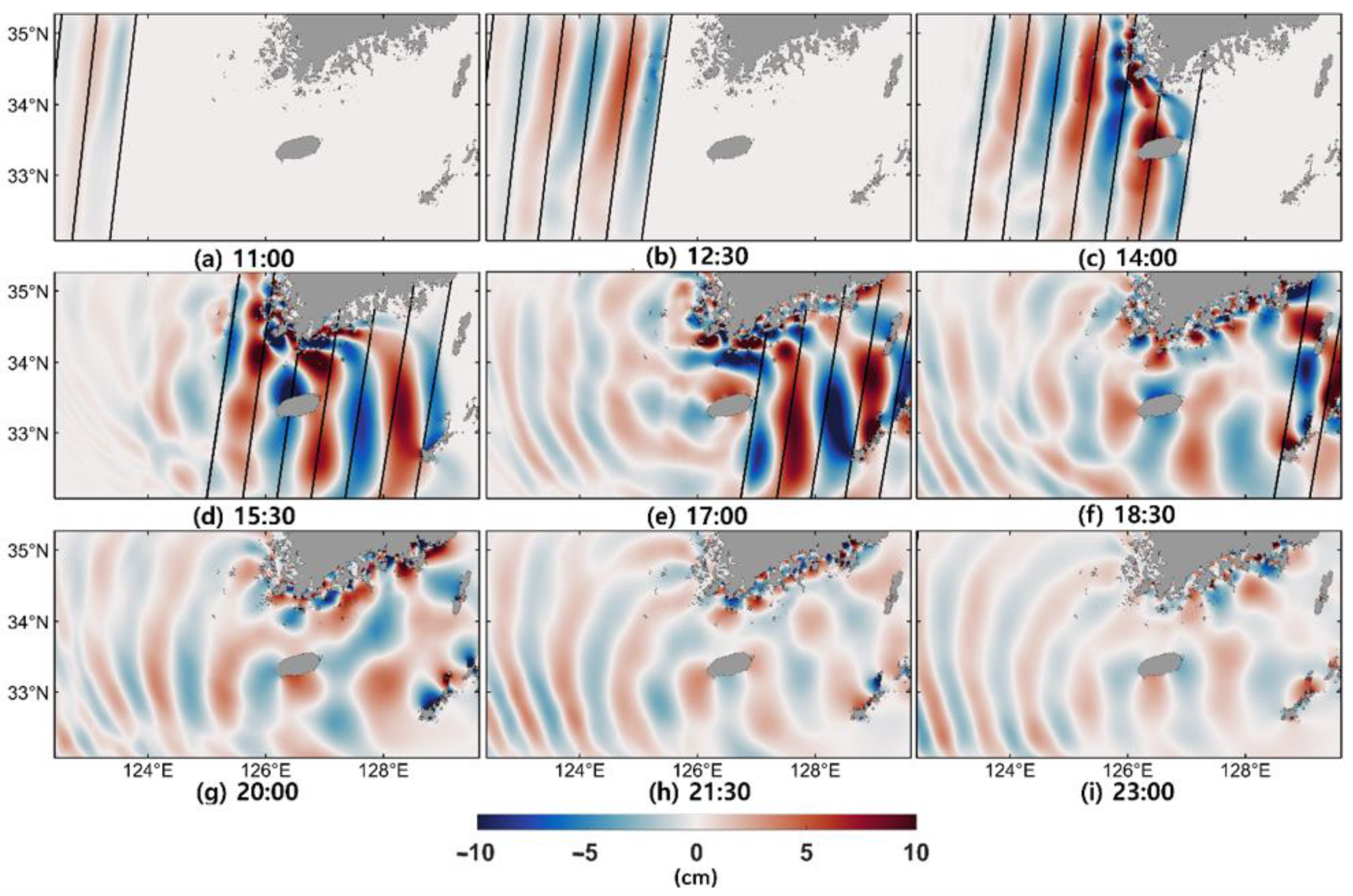
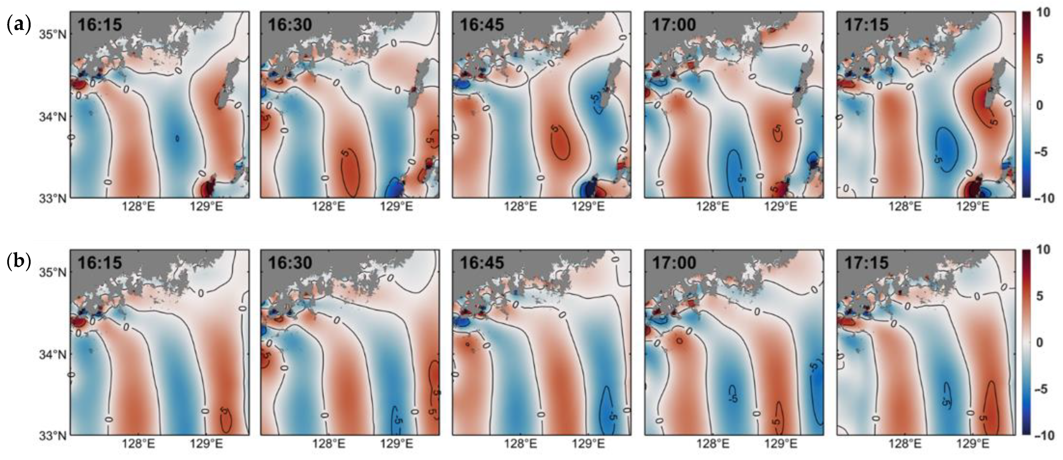
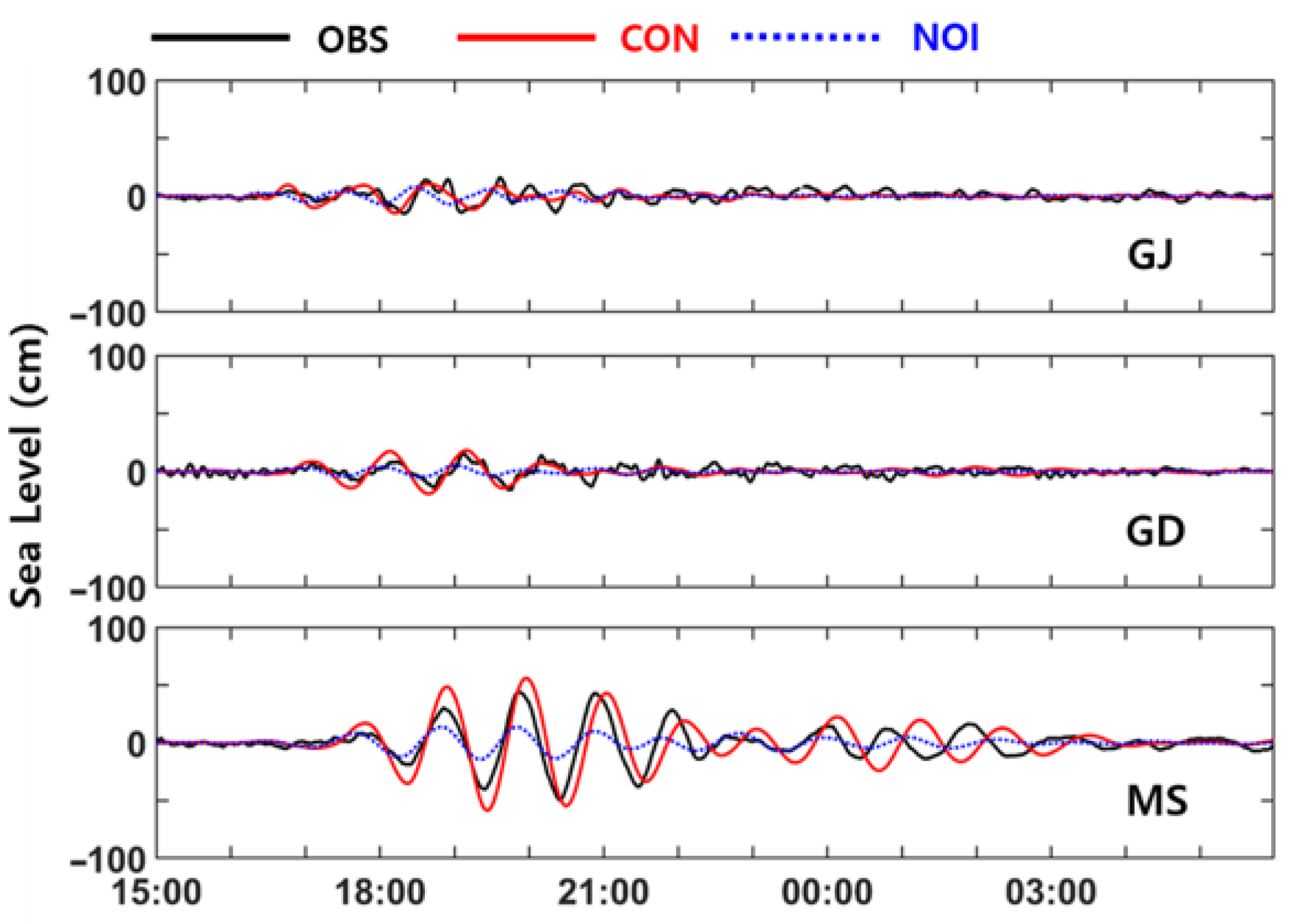
3.2. Numerical Simulations

The generation and propagation process of long ocean waves in the Korea Strait was investigated using a two-dimensional numerical model. A simple form of atmospheric pressure forcing was constructed based on the observational data for the numerical simulations. An ensemble of atmospheric pressure disturbances with different amplitudes, moving speeds, angles, shapes, and periods was tested to reproduce the observed sea level oscillations along the coast in the Korea Strait. In this study, a single realization, which fitted the sea level oscillations along the Korea Strait on 7 April 2019, is presented. Atmospheric pressure disturbances propagated eastward along the Korea Strait and consisted of three sinusoidal plane waves based on the observation data (Figure 5). The amplitude, period, movement speed ( U ), and angle (θ) of the atmospheric pressure disturbances were assumed to be 1 hPa, 60 min, 30 m/s, and 80° counterclockwise due east, respectively. The shape of atmospheric disturbances changes in time and space, and idealized sinusoidal waves were used in the numerical experiment (Figure 2 and Figure 3a,c). Most of other previous studies also used approximate disturbances (i.e., idealized shapes, such as step function, triangle, and sinusoidal wave) [15,18,28,29]. Their shape and moving speed do not change in time like in our study. However, they are localized disturbances moving in time. When one or two sinusoidal waves of atmospheric disturbances were propagated eastward, the duration of the long ocean wave event was shorter, and the number of long ocean waves was smaller than the observation data. When four sinusoidal waves of atmospheric disturbances were moving, the duration of the long ocean wave event was longer than the observation. The period of the long ocean waves increased with the period of the sinusoidal atmospheric disturbances, whereas the amplitude of the long ocean waves was nearly invariant except at the MS tide observation station. The numerical simulations in this study are idealized ones in terms of atmospheric forcing and initial conditions.
The time series of the atmospheric pressure forcing used for the numerical simulations and those of the observed atmospheric pressure data were compared at SGP, GH, and MS (Figure 6a). The atmospheric pressure forcing at SGP and GH, which are located to the southwest and north of the Korea Strait, respectively, had two and three peaks from 13:50 to 17:10 on 7 April. The amplitude and phase of the first peaks were different at SGP, although the second and third peaks had a similar amplitude and phase. At GH, the phases of the first peak were coincident but the amplitudes were different, and the amplitudes of the second and third waves were similar but the model forcing lagged behind the observed atmospheric pressure variation. The atmospheric pressure anomaly had similar wave amplitudes at MS but was out of phase between the model forcing and the observation. The atmospheric pressure disturbances from the observation kept changing in time and space (Figure 3a); therefore, the simple sinusoidal form of model atmospheric pressure forcing could not match the irregular observed atmospheric pressure disturbances. However, the packets or trains of atmospheric pressure disturbances were relatively similar at SGP, GH, and MS in terms of beginning time, end time, and amplitude (Figure 6a).
The simulated sea level variations were compared with sea level observation data that were high-pass-filtered with a cutoff period of 180 min (Figure 6b). The numerical model reproduced the amplitude and phase of sea level oscillations similar to the observation at SGP, GH, and MS. There were time lags between the simulated and the observed sea level anomalies. The lags of simulated sea level variations were −1, −4, and +3 min compared with the observations at SGP, GH, and MS, respectively. The time-lagged correlation coefficients over 6 h were 0.53, 0.37, and 0.89 at SGP, GH, and MS, respectively, and the RMSEs were 5.38, 10.78, and 19.70 cm at SGP, GH, and MS, respectively. As the pressure disturbances moved to the east (black solid lines in Figure 7), long ocean waves were generated due to Proudman resonance in the southwestern Yellow Sea. The amplitude of the long ocean waves kept growing while they propagated, in addition to pressure disturbances in the relatively deep region of 122.5–126.0° E and 33.5–35.0° N (Figure 7a,c). The long ocean waves were refracted due to the bottom topography, where the water depth was less than about 75 m ( Fr ≤ 0.9), and lagged behind the pressure disturbances (Figure 7c,d). However, the long ocean waves propagated ahead of the atmospheric pressure disturbances where the water depth was deeper than 108 m ( Fr ≥ 1.1) (Figure 7d). Reflected waves were generated and propagated westward, while the forced long ocean waves (meteotsunami) propagated eastward (Figure 7d,e). As the long ocean waves reached the shallow coastal region or islands, they refracted and reflected (Figure 7c,e). Even after the pressure disturbances moved out of the model domain, the sea level continued to oscillate due to the waves reflecting from the coast (Figure 7g,i). The start times of sea level oscillations at SGP were similar to the arrival times of the trains of atmospheric pressure disturbances, whereas sea level oscillations started 1–3 h after the arrival times of atmospheric pressure disturbances at GH and MS (Figure 6). The reason the arrival of long ocean waves was delayed at GH and MS is that the propagation of long ocean waves is slowed down as they refract in the coastal region due to the shallow water (Figure 7c,d).

4. Discussion

4.1. Proudman and Greenspan Resonances

Long ocean waves are amplified by three resonance processes in the shallow coastal ocean: Proudman, Greenspan, and shelf resonances [3,4]. When a long ocean wave enters a bay or an estuary, its wave height may be amplified due to shoaling and harbor resonance. As atmospheric disturbances move eastward with speeds of 20.0–31.0 m/s over the southern Yellow Sea toward the Korea Strait (Figure 2 and Table 1), Proudman resonance amplifies long ocean waves, where the bottom depth is between 40.1 and 91.7 m (Figure 1 and Figure 7). These eastward-moving atmospheric pressure disturbances amplify long ocean waves by Proudman resonance in an offshore region deeper than 45 m in the southern Yellow Sea (Figure 7). As the long ocean waves cross 126° E and enter the Korea Strait, they lag behind the atmospheric pressure disturbances, moving eastward in the shallow region near the coast, and the wave crests tend to become parallel to the coast due to refraction (Figure 7 and Figure 8). However, the long ocean waves offshore and deeper than 100 m keep accompanying the moving atmospheric pressure disturbances and grow in amplitude.
Greenspan resonance occurs when the propagation speed of an atmospheric disturbance is close to that of edge waves, coastal trapped waves over a sloping shelf that propagate along the coast [30]. The speed of an edge wave ( C e w ) is given as:
C e w = g T tan [ ( 2 n + 1 ) β ] / 2 π
where g is the acceleration due to gravity, n is an integer for each mode, β is the bottom slope, and T is the wave period [31]. Based on the bottom slope ( β ) of 0.00103–0.00224 from CJ to GD along the 50 m isobath in the northern Korea Strait and the observed wave period of 60 min, the estimated edge wave speeds are 6–13 m/s for n = 0 and 17.0–38.0 m/s for n = 1. It may be possible that the eastward propagation speed (21–31 m/s) of the atmospheric pressure disturbances is close to the trapped edge wave speeds, and the long waves grow by Greenspan resonance [4,28].

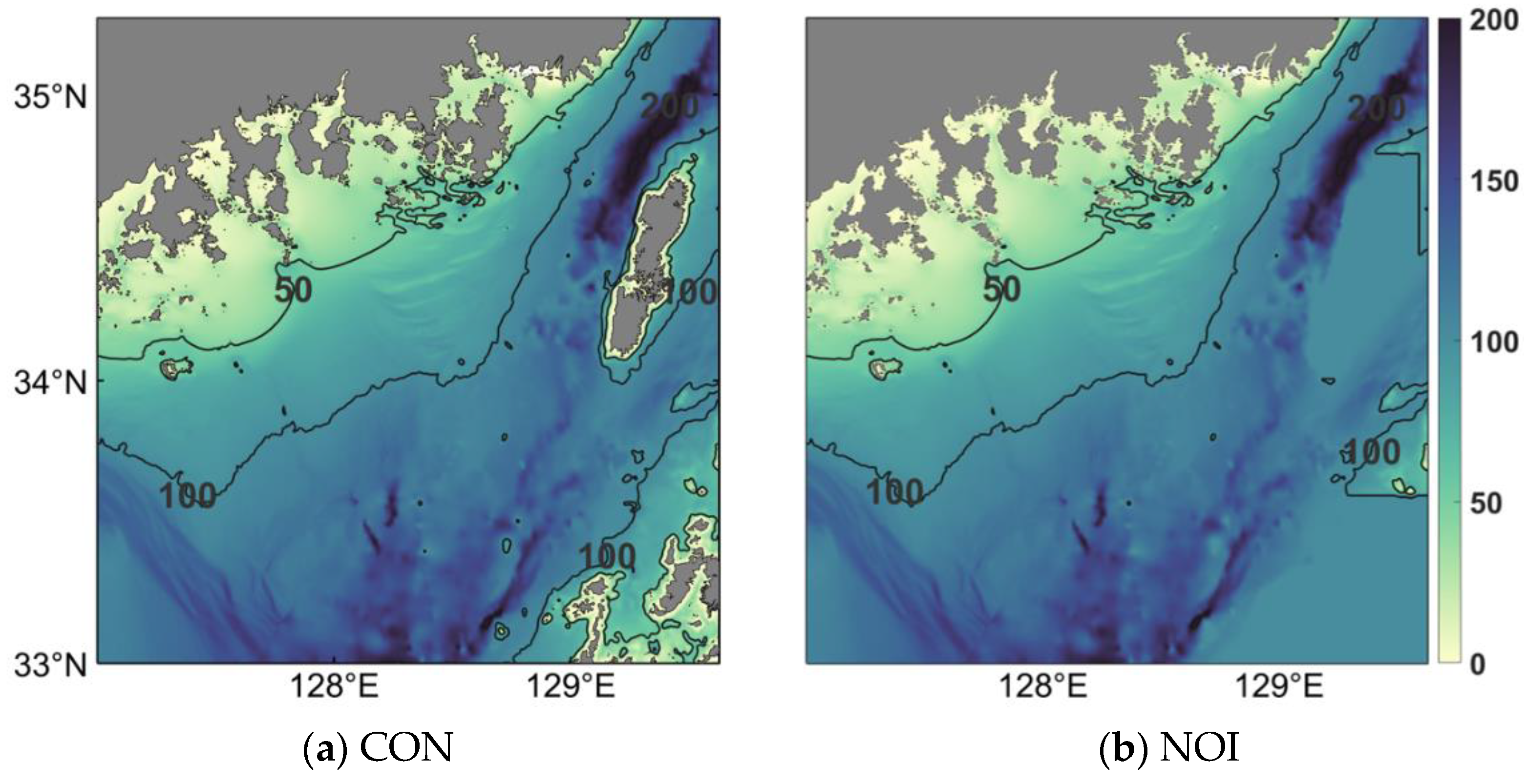
4.2. Refraction and Reflection by Offshore Islands

The sea level oscillations at MS in Jinhae-Masan Bay had relatively large amplitudes from both observations and numerical simulations among the tide gauge stations in the Korea Strait (Figure 3 and Figure 7 and Table 2). The superposition of waves propagating northeastward along the coast of the Korea Strait and waves refracted and reflected by bottom topography and Tsushima Island increased the wave energy entering Jinhae-Masan Bay (Figure 7e,g). To examine the effects of refraction and reflection due to bottom topography and Tsushima Island on the waves entering Jinhae-Masan Bay, a numerical model simulation was performed without the islands under the same atmospheric pressure forcing (NOI experiment). After removing the islands from the model domain, the bottom topography where the islands had been was made similar to the surrounding region (Figure 8).
The distribution of the sea level at 16:30 indicated that wave heights between GJ and Tsushima Island were higher in the control (CON) experiment than in the NOI experiment (Figure 9b). A trough of long ocean waves propagated through the mouth of Jinhae-Masan Bay at 16:30. The long ocean wave refracted and reflected by the islands formed a wave crest parallel to the coast in the CON experiment at 16:45, whereas the wave crest was perpendicular to the coast in the NOI experiment (Figure 9b). Then, the crest of the long ocean wave entered the mouth of Jinhae-Masan Bay at 17:00 (Figure 7e and Figure 9) and propagated toward MS at 17:15. The distribution of sea level at 16:15 was similar to that at 17:15, but had an opposite phase to that at 16:45 in both numerical simulations. In the NOI experiment, most of the long ocean wave energy propagated to the east along the coast instead of entering Jinhae-Masan Bay (Figure 9b).
To examine the role of the refracted and reflected waves on sea level variation in Jinhae-Masan Bay, sea level variations from the numerical simulations were compared with the observed sea level variations at GJ, GD, and MS (Figure 10). The sea level oscillations in the CON experiment started at 16:46, 17:05, and 17:48 at GJ, GD, and MS, respectively. The sea level oscillations in the NOI experiment started at 16:38, 16:57, and 17:40, respectively, which were 8 min earlier than those in the CON experiment. When the amplitudes of sea level oscillations were compared over 6 h from the beginning of the long wave event, the wave amplitudes at GJ, GD, and MS were 34.2%, 67.8%, and 72.7% larger in the CON experiment than those in the NOI experiment, respectively. The numerical experiments revealed that the refraction and reflection of waves by the offshore island and bottom topography affect amplitudes and arrival times of the long wave in Jinhae-Masan Bay. In [15], it is suggested that the interaction between long waves and tides in the Yellow Sea affects the arrival time and amplitude of long ocean waves. Therefore, the interaction between long waves and tides may need to be considered to increase the accuracy in the prediction of amplitudes and arrival times of long ocean waves in the Korea Strait.

4.3. Local Topographic Effects

As a long ocean wave generated by Proudman resonance propagate in the ocean, it can be amplified by Greenspan, shelf, and harbor resonances due to local bathymetric characteristics [5]. SGP and GH are located in the west, and MS is in the east of the Korea Strait (Figure 1). The long waves arriving at SGP and GH were amplified in the southeastern Yellow Sea, whereas the long ocean waves arriving at MS propagated through the Korea Strait and entered Jinhae-Masan Bay (Figure 3 and Figure 11). The tide observation stations at SGP and GH are located at an open coast. However, the MS tide observation station is located in an elongated bay, Jinhae-Masan Bay. Before the long ocean waves entered Jinhae-Masan Bay, they were amplified and refracted in the Korea Strait. After the long waves entered Jinhae-Masan Bay, their amplitudes were increased by shoaling and harbor resonance [18,22]. MS is almost in the innermost part of the elongated narrow bay (Figure 11). The distance and average depth from the 40 m isobath offshore to the MS tide observation station are approximately 40 km and 24 m, respectively. The periods of natural harbor resonance for a semienclosed bay are given as:
T n =   4 l ( 2 n 1 )   g h                   n = 1 ,   2 ,   3 ,  
where T n is the resonant harbor oscillation period of the n-th mode for a semienclosed bay. l and h are the length and average depth of a bay, respectively. g is gravitational acceleration. The resonance periods ( T n ) in Jinhae-Masan Bay are 174, 58, and 35 min for n = 1, 2, and 3, respectively. The theoretical periods of the second and third modes ( n = 2 and 3) in sea level oscillations are within the observed periods of 35–90 min at the MS tide observation station (Figure 4). In [22], it is assumed that the length and averaged depth of the inner bay from 35.08° N to the MS tidal station are 13.1 km and 10.6 m, respectively (Figure 11c). They suggested that the natural resonance periods of the inner bay are 85.6 and 28.5 min for n = 1 and 2.

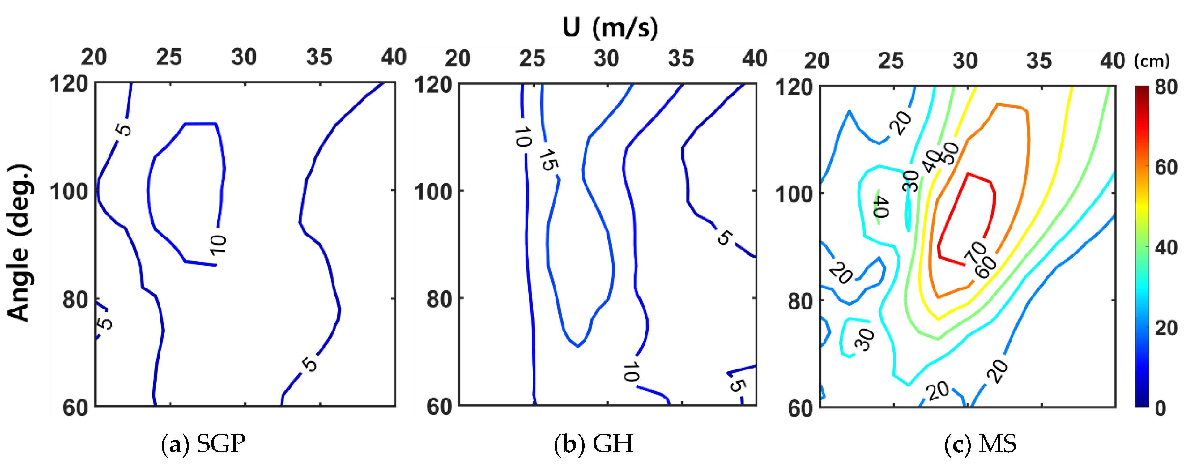
4.4. Effects of Speed and Angle of the Atmospheric Pressure Disturbances

Even if the amplitude of atmospheric pressure disturbance is the same, the amplitude of a long ocean wave generated by the moving atmospheric pressure disturbance depends on the propagating speed and angle of atmospheric pressure jumps in a coastal region [15,28,29]. Changes in long ocean wave amplitude are caused by the refraction, reflection, and shoaling of propagating long ocean waves due to variations in bottom topography and the coastline. To estimate changes in the amplitude of long ocean waves with respect to the propagation speed and angle of atmospheric pressure disturbances in the Korea Strait (Figure 5), numerical experiments forced by atmospheric pressure disturbances moving with speeds of 20–40 m/s and angles of 60–120° were performed (Figure 12). In these experiments, atmospheric disturbance was assumed as an idealized sine wave propagating eastward with an amplitude of 1 hPa and a period of 60 min. When such air pressure jumps move from the west to the east along the Korea Strait, the ranges of long ocean wave amplitudes at SGP, GH, and MS are 3–12, 4–19, and 17–76 cm, respectively. The eastward-moving atmospheric pressure jumps with velocities of 27–34 m/s and angles of 80°–118° make the amplitude of the long ocean wave higher than other atmospheric pressure jumps. The amplitude of long ocean waves arriving at SGP and GH is less sensitive to the moving speed and angle of atmospheric pressure disturbances than that at MS. When the speed of eastward-moving atmospheric pressure disturbances is between 24 and 30 m/s, Proudman resonance effectively enhances the long wave amplitude in the southwestern Yellow Sea and East China Sea, and the amplitude of long waves observed at SGP and GH increases. However, the amplitude of long waves observed at MS would reach a maximum when the eastward-moving speed and angle of atmospheric pressure disturbance are 30 m/s and 85–100°, respectively. Such selective and sensitive responses of the sea level at MS may be related to the bottom topography of the Korea Strait and harbor resonance within Jinhae-Masan Bay.
The expected amplitude of long waves at each station in Figure 12 can be used to predict the amplitude of long ocean waves when the eastward-moving speed and direction of atmospheric pressure isobars are detected in the real-time monitoring system. For future study, it will be necessary to investigate the generation of meteotsunamis in the Korea Strait when atmospheric pressure disturbances propagate from south to north across the strait, such as in a long ocean wave event in March 2014 [22], using observation data and numerical experiments.

5. Conclusions

In this work, long ocean waves (meteotsunami) propagating from southwest to northeast along the Korea Strait were observed, while atmospheric pressure disturbances moved from west to east on 7 April 2019. The amplification of long ocean waves by Proudman resonance in the Korea Strait was demonstrated in this study for the first time. The moving speed of atmospheric pressure disturbances was 26.5–31.0 m/s with an inclination of 75–83° in the counterclockwise direction. The average height of the atmospheric pressure disturbance was 2.4 hPa, and two to four waves passed in succession.
The two-dimensional numerical simulation reproduced the propagation of long ocean waves in the Korea Strait. The arrival time, phase, and period of the simulated long ocean waves were appropriately estimated to within a few minutes. The long ocean waves were generated due to Proudman resonance as the atmospheric pressure disturbances moved over the Yellow Sea and East China Sea. The maximum amplitude of sea level fluctuation was 16.3–91.9 cm. The amplification of sea level oscillations was highest at Masan (MS) due to reflection from an island and the shoaling effect. After the long wave hit the coast of the Korea Strait, the sea level oscillated continuously for 7–19 h with 10–160 min periods. The long ocean waves responded immediately to atmospheric pressure disturbances in the open sea, but they reacted 1–3 h later in the coasts and bays of the Korea Strait. The propagation speed of a long ocean wave was slowed down by shallow topography in the coast, and refraction was caused by complex topography, coastlines, and islands. The reason for the small amplitude of sea level oscillations in coastal areas except for MS was that a long ocean wave propagated parallel to the isobath; thus, the shoaling effect was small. At MS, the amplitude of sea level fluctuation was largest due to the combination of the refraction, the reflection by the islands, harbor resonance, and the shoaling effect as energy entered the bay. The contribution of reflected waves by islands was 72.7% for sea level oscillations of MS. We could determine the high sea level oscillation conditions in the Korea Strait through sensitivity experiments with different moving velocities and angles. These results will be useful for the development of real-time monitoring and prediction systems for meteotsunami.

Author Contributions

Conceptualization, B.-J.C. and K.K.; methodology, B.-J.C. and S.-G.M.; validation, K.K., S.-G.M., and H.-S.S.; formal analysis, B.-J.C. and S.-G.M.; data curation, H.-S.S.; writing—original draft preparation, K.K.; writing—review and editing, B.-J.C. and K.K.; visualization, S.-G.M. and H.-S.S.; supervision, B.-J.C. All authors have read and agreed to the published version of the manuscript.

Funding

This research was part of a project titled “Improvements of ocean prediction accuracy using numerical modeling and artificial intelligence technology” funded by the Ministry of Oceans and Fisheries, Korea, and supported by the Basic Science Research Program through the National Research Foundation of Korea (NRF) funded by the Ministry of Education (NRF-2020R1A2C1014678).

Institutional Review Board Statement

Not applicable.

Informed Consent Statement

Not applicable.

Data Availability Statement

Not applicable.

Acknowledgments

The authors would like to thank the Korea Meteorological Administration (KMA) and the Korea Hydrographic and Oceanographic Agency (KHOA) for the dataset.

Conflicts of Interest

The authors declare no conflict of interest.

References

  1. Monserrat, S.; Vilibić, I.; Rabinovich, A.B. Meteotsunamis: Atmospherically induced destructive ocean waves in the tsunami frequency band. Nat. Hazards Earth Syst. Sci. 2006, 6, 1035–1051. [Google Scholar] [CrossRef]
  2. Rabinovich, A.B. Twenty-Seven Years of Progress in the Science of Meteorological Tsunamis Following the 1992 Daytona Beach Event. Pure Appl. Geophys. 2020, 177, 1193–1230. [Google Scholar] [CrossRef]
  3. Proudman, J. The effects on the sea of changes in atmospheric pressure. Geophys. Suppl. Mon. Not. R. Astron. Soc. 1929, 2, 197–209. [Google Scholar] [CrossRef]
  4. Greenspan, H.P. The generation of edge waves by moving pressure distributions. J. Fluid Mech. 1956, 1, 574–592. [Google Scholar] [CrossRef]
  5. Pattiaratchi, C.B.; Wijeratne, E.M.S. Are meteotsunamis an underrated hazard? Philos. Trans. R. Soc. A Math. Phys. Eng. Sci. 2015, 20140377. [Google Scholar] [CrossRef] [PubMed] [Green Version]
  6. Renault, L.; Vizoso, G.; Jansá, A.; Wilkin, J.; Tintoré, J. Toward the predictability of meteotsunamis in the Balearic Sea using regional nested atmosphere and ocean models. Geophys. Res. Lett. 2011, 38, L10601. [Google Scholar] [CrossRef] [Green Version]
  7. Vilibic, I. Numerical simulations of the Proudman resonance. Cont. Shelf. Res. 2008, 28, 574–581. [Google Scholar] [CrossRef]
  8. Vilibić, I.; Šepić, J.; Rabinovich, A.B.; Monserrat, S. Modern Approaches in Meteotsunami Research and Early Warning. Front. Mar. Sci. 2016, 3, 57. [Google Scholar] [CrossRef] [Green Version]
  9. Bailey, K.; DiVeglio, C.; Welty, A. An Examination of the June 2013 East Coast Meteotsunami Captured by NOAA Observing Systems. NOAA Technical Report; 2014; pp. 1–42. Available online: https://repository.library.noaa.gov/view/noaa/14435 (accessed on 20 August 2021).
  10. Šepić, J.; Vilibić, I.; Rabinovich, A.B.; Monserrat, S. Widespread tsunami-like waves of 23-27 June in the Mediterranean and Black Seas generated by high-altitude atmospheric forcing. Sci. Rep. 2015, 5, 11682. [Google Scholar] [CrossRef] [Green Version]
  11. Raichlen, F. Harbor resonance. In Estuary and Coastline Hydrodynamics, 1st ed.; Eagleson, P.S., Ippen, A.T., Eds.; McGraw Hill Book Co.: New York, NY, USA, 1966; pp. 281–340. [Google Scholar]
  12. Mei, C.C. The Applied Dynamics of Ocean Surface Waves, 2nd ed.; World Scientific: London, UK, 1992; p. 740. [Google Scholar]
  13. Wilson, B. Seiches. Adv. Hydrosci. 1972, 8, 1–94. [Google Scholar] [CrossRef]
  14. Miles, J.W. Harbor seiching. Ann. Rev. Fluid Mech. 1974, 6, 17–36. [Google Scholar] [CrossRef]
  15. Choi, B.-J.; Hwang, C.; Lee, S.-H. Meteotsunami-tide interactions and high-frequency sea level oscillations in the eastern Yellow Sea. J. Geophys. Res. Ocean. 2014, 119, 6725–6742. [Google Scholar] [CrossRef]
  16. Ozsoy, O.; Haigh, I.D.; Wadey, M.P.; Nicholls, R.J.; Wells, N.C. High-frequency sea level variations and implications for coastal flooding: A case study of the Solent, UK. Cont. Shelf Res. 2016, 122, 1–13. [Google Scholar] [CrossRef] [Green Version]
  17. Vilibić, I.; Rabinovich, A.B.; Anderson, E.J. Special issue on the global perspective on meteotsunami science: Editorial. Nat. Hazards 2021, 106, 1087–1104. [Google Scholar] [CrossRef]
  18. Hibiya, T.; Kajiura, K. Origin of the Abiki phenomenon (a kind of seiche) in Nagasaki Bay. J. Oceanogr. Soc. Jpn. 1982, 38, 172–182. [Google Scholar] [CrossRef]
  19. Tanaka, K. Atmospheric pressure-wave bands around a cold front resulted in a meteotsunami in the East China Sea in February 2009. Nat. Hazards Earth Syst. Sci. 2010, 10, 2599–2610. [Google Scholar] [CrossRef] [Green Version]
  20. Heo, K.-Y.; Yoon, J.-S.; Bae, J.-S.; Ha, T. Numerical Modeling of Meteotsunami-Tide Interaction in the Eastern Yellow Sea. Atmosphere 2019, 10, 369. [Google Scholar] [CrossRef] [Green Version]
  21. Kim, M.-S.; Eom, H.; You, S.H.; Woo, S.-B. Real-time pressure disturbance monitoring system in the Yellow Sea: Pilot test during the period of March to April 2018. Nat. Hazards 2021, 106, 1703–1728. [Google Scholar] [CrossRef]
  22. Park, S.J.; Choi, B.-J.; Sim, H.S.; Byun, D.-S. Arrival of Long Ocean Waves and Hourly Sea Level Oscillations in Masan Bay, Korea on 19–22 March 2014. J. Coast. Res. 2020, 95, 1510–1514. [Google Scholar] [CrossRef]
  23. Haidvogel, D.B.; Arango, H.G.; Hedstrom, K. Model evaluation experiments in the North Atlantic Basin: Simulations in nonlinear terrain-following coordinates. Dynam. Atmos. Oceans 2000, 32, 239–281. [Google Scholar] [CrossRef]
  24. Shchepetkin, A.F.; McWilliams, J.C. The regional oceanic modeling system (ROMS): A split-explicit, free-surface, topography-following-coordinate oceanic model. Ocean Model. 2005, 9, 347–404. [Google Scholar] [CrossRef]
  25. Seo, S.-N. Digital 30sec gridded bathymetric data of Korea marginal seas—KorBathy30s. J. Korean Soc. Coast. Ocean. Eng. 2008, 20, 110–120. (In Korean) [Google Scholar]
  26. Chapman, D.C. Numerical treatment of cross-shelf open boundaries in a barotropic coastal ocean model. J. Phys. Oceanogr. 1985, 15, 1060–1075. [Google Scholar] [CrossRef] [Green Version]
  27. Flather, R.A. A tidal model of the northwest European continental shelf. Mem. Soc. R. Sci. Liege. 1976, 6, 141–164. [Google Scholar]
  28. Bechle, A.J.; Wu, C.H. The Lake Michigan meteotsunamis of 1954 revisited. Nat. Hazards 2014, 74, 155–177. [Google Scholar] [CrossRef]
  29. Williams, D.A.; Horsburgh, K.J.; Schultz, D.M.; Hughes, C.W. Examination of Generation Mechanisms for an English Channel Meteotsunami: Combining Observations and Modeling. J. Phys. Oceanogr. 2019, 49, 103–120. [Google Scholar] [CrossRef]
  30. Donn, W.L.; Ewing, M. Stokes’ edge waves in Lake Michigan. Science 1956, 124, 1238–1242. [Google Scholar] [CrossRef]
  31. Ursell, F. Edge waves on a sloping beach. Proc. R. Soc. Lond. Ser. A Math. Phys. Sci. 1952, 214, 79–98. [Google Scholar] [CrossRef]
Figure 1. (a) The red dashed rectangle represents the study area covering the Korea Strait between the Yellow Sea, East China Sea, and East Sea. (b) Observation stations for atmospheric pressure (red) and sea level (yellow) in the Korea Strait. CJ, SGP, GM, GH, YS, GJ, GD, MS, SSB, and HKT stand for Chujakdo, Seogwipo, Geomundo, Goheung, Yeosu, Geojedo, Gadeokdo, Masan, Sasebo, and Hakata, respectively. Contours represent the bottom topography (m). Jeju Island and Tsushima Island are located at 126.8° E, 33.4° N and 129.5° E, 34.5° N, respectively, in the Korea Strait. MS is located in Jinhae-Masan Bay (128.4–128.8° E, 34.9–35.3° N).
Atmosphere 12 01083 g001
Figure 2. Rainfall intensity (mm/h) estimated from rainfall radar at (a) 15:00, (b) 16:30, (c) 18:00, and (d) 19:30 on 7 April 2019.
Atmosphere 12 01083 g002
Figure 3. Variations of (a) atmospheric pressure (hPa) and (b) sea levels (cm), which were high-pass-filtered with a cutoff period of 180 min. (c) Arrival times (hour:minute) of atmospheric pressure disturbances and (d) the long ocean waves (meteotsunami) along the Korea Strait on 7 April 2019. The contour intervals are 30 min. The dashed green contour lines in (c,d) are the extrapolated locations of atmospheric pressure disturbance and long ocean wave, respectively, based on the patterns of nearby observation data.
Atmosphere 12 01083 g003
Figure 4. Wavelet spectrum of (a) atmospheric pressure and (b) sea level time series at the SGP, GH, and MS stations from 12:00 on 7 April to 12:00 on 8 April 2019.
Atmosphere 12 01083 g004
Figure 5. Eastward propagation of atmospheric pressure disturbances with a moving speed ( U ) and angle (θ) at 13:00 on 7 April 2019. The angle of a moving isobar was measured counterclockwise due east. The arrow represents the moving direction of the atmospheric pressure disturbances. The waves under the arrow represent a schematic sinusoidal form of the atmospheric pressure disturbances.
Atmosphere 12 01083 g005
Figure 6. Comparison of (a) atmospheric pressure anomalies and (b) sea level variations from observations and numerical simulations at SGP, GH, and MS from 12:00 on 7 April to 06:00 on 8 April 2019.
Atmosphere 12 01083 g006
Figure 7. Spatial distribution of modeled sea level elevation (colors) in the Yellow Sea and Korea Strait every 1.5 h from 11:00 to 23:00 on 7 April 2019. Colors represent sea level anomalies. Black straight lines represent 1024 hPa isobars in atmospheric pressure that propagate eastward (Figure 5).
Atmosphere 12 01083 g007
Figure 8. Spatial distributions of bottom depth (m) for (a) the control (CON) experiment and (b) no offshore islands (NOI) experiment. The contour intervals of the isobaths are 50 m.
Atmosphere 12 01083 g008
Figure 9. Spatial distributions of surface elevation every 15 min from 16:15 to 17:15 on 7 April 2019. The upper and lower panels are (a) surface elevation from the original topography (CON) and (b) no offshore island (NOI) models, respectively. The contour intervals of surface elevation are 5 cm.
Atmosphere 12 01083 g009
Figure 10. Sea level variations from the observation (black line), original topography model (CON; red line), and no offshore island model (NOI; blue dotted line) at GJ, GD, and MS from 15:00 on 7 April to 06:00 on 8 April 2019.
Atmosphere 12 01083 g010
Figure 11. Enlarged topographic maps of the (a) SGP, (b) GH, and (c) MS tide observation stations. Colors represent bottom depths in meter. The bottom topography is contoured at depths of 10, 20, 50 and 100 m.
Atmosphere 12 01083 g011
Figure 12. Expected amplitudes (cm) of the long ocean waves at (a) SGP, (b) GH, and (c) MS in the Korea Strait if an atmospheric pressure disturbance propagated eastward with various isobar angles (θ in Figure 5) and traveling speeds ( U ) from 20 to 40 m/s.
Atmosphere 12 01083 g012
Table 1. Start time and maximum height (ΔP) of atmospheric pressure disturbances at the coastal stations on 7 April 2019. Δt is the corresponding elapsed time in the change of atmospheric pressure (ΔP). Intervals of atmospheric pressure data at SSB and HKT are 10 min and their station name, arrival time, Δt, and ΔP are in italics.
StationArrival Times (Hour:Minute)Δt (Minutes)ΔP (hPa)
CJ13:49593.9
SGP14:29342.6
GH14:15172.1
GM14:50172.0
YS14:33122.1
GJ15:58291.9
MS15:46261.5
GD16:21332.5
SSB17:35712.7
HKT18:15662.7
Table 2. Arrival times and maximum wave heights of long ocean waves at the tide gauge stations in the Korea Strait.
StationArrival Time (Hour:Minute)Maximum Wave Height (cm)
CJ13:5938.1
SGP14:1426.6
GH15:0742.5
GM14:5616.3
YS15:4829.7
GJ16:4730.1
MS17:4891.9
GD17:0530.1
SSB17:1838.6
HKT20:0839.0
Publisher’s Note: MDPI stays neutral with regard to jurisdictional claims in published maps and institutional affiliations.

