Research on Monthly Precipitation Prediction Based on the Least Square Support Vector Machine with Multi-Factor Integration

Abstract

Accurate precipitation prediction is of great significance for regional flood control and disaster mitigation. This study introduced a prediction model based on the least square support vector machine (LSSVM) optimized by the genetic algorithm (GA). The model was used to estimate the precipitation of each meteorological station over the source region of the Yellow River (SRYE) in China for 12 months. The Ensemble empirical mode decomposition (EEMD) method was used to select meteorological factors and realize precipitation prediction, without dependence on historical data as a training set. The prediction results were compared with each other, according to the determination coefficient (R²), mean absolute errors (MAE), and root mean square error (RMSE). The results show that sea surface temperature (SST) in the Niño 1 + 2 region exerts the largest influence on accuracy of the prediction model for precipitation in the SRYE (${\mathrm{R}}_{\mathrm{SST}}^2=$ 0.856, ${\mathrm{RMSE}}_{\mathrm{SST}}=$ 19.648, ${\mathrm{MAE}}_{\mathrm{SST}}=$ 14.363). It is followed by the potential energy of gravity waves (Ep) and temperature (T) that have similar effects on precipitation prediction. The prediction accuracy is sensitive to altitude influences and accurate prediction results are easily obtained at high altitudes. This model provides a new and reliable research method for precipitation prediction in regions without historical data.

1. Introduction

The source region of the Yellow River (SRYE), located in the northeast of the Qinghai-Tibet Plateau, China, is a key region closely related to adverse weather events in the eastern, southern, and northern regions of China. The SRYE contributes a considerable amount of water to the lower reaches of the Yellow River, with an average annual water supply of 2 × 10¹⁰ m³. The source region of the Yellow River is located on the edge of the East Asian monsoon; the inhomogeneity of the temporal and spatial distribution of precipitation has caused frequent occurrences of droughts and floods in the middle and lower reaches of the Yellow River. Accurate precipitation prediction is of great significance for flood control and disaster mitigation. However, precipitation has a high degree of nonlinearity, randomness, and complexity, and is affected by environmental factors, such as terrain, air pressure, circulation, etc., which lowers the accuracy of precipitation prediction. In recent years, with the rapid development of artificial intelligence technology, artificial intelligence methods have greatly improved the accuracy of precipitation forecasts. The main task of this research was to predict precipitation at 18 ground-based meteorological stations in the SRYE and quantify the influences of different driving forces of precipitation.

In recent years, data-driven methods based on artificial intelligence technology have been widely used to estimate and predict global precipitation. The support vector machine (SVM) learning algorithm, based on the statistical learning theory and the mapping theory of kernel function, is a typical machine-learning algorithm for small samples. It has been widely applied in the field of hydrology and water resources, such as runoff prediction and evaluation on water quality [1,2]. However, these models need (a lot of) accurate data for parameter calibration; it is difficult to quantify a temporal-spatial structure of rich precipitation with a long-term dependence. In fact, it is hard to obtain sufficient and accurate data in some regions not investigated, which leads to poor performance and high uncertainty of the models [3]. Other relatively mature methods, such as the least square support vector machine regression (LSSVR), are often used in hydrology and climate research [4,5,6,7]. They perform excellently in modeling complex processes and make up for the shortage of excessive noise in short data sets [8,9]. These advantages, of data-driven methods, make them suitable for modeling hydrological and climatic processes. Many studies have reported the successful application of data-driven methods in the modeling of hydrological and climatic processes, such as precipitation, rainfall runoff, runoff, evapotranspiration, water quality, and drought, revealing the capacity of these methods in modeling complex processes [10,11,12,13,14,15,16,17]. However, such methods do not usually involve the physical mechanisms and laws behind the data, so it is difficult to deeply analyze the hydrological and climatic processes [18]. To date, many studies have been carried out to compare the performances of different types of data-driven methods in modeling and forecasting of hydrometeorological variables [19,20]. The atmospheric circulation has a significant impact on precipitation, and the persistent circulation system will cause long-term precipitation events [21]. Previous research shows that the increase of carbon dioxide concentration and the atmospheric circulation affect the spatial pattern of precipitation over the tropical Pacific [22]. Using climate model projections in the 21st century, tropical circulation slows down [23], which leads to an increase in the growth rate of global average rainfall (every 2–3% temperature rise on the surface of the earth). The study demonstrates that North Atlantic Oscillation (NAO) index and Western Pacific Oscillation (WPO) index are negatively correlated with average precipitation over the Siberia and Central Asia [24]. Many numerical modes and statistical regression analysis methods have proven the role of the topographic effect on precipitation, and its influence on the distribution of precipitation has been researched from geographical and topographical factors [25,26,27,28,29,30,31]. A mountain range is the main cause of atmospheric gravity waves propagating to high altitudes. The waves generating by convection is further mixed in the lower troposphere, which is conducive to transporting water vapors to the upper layer of the Qinghai-Tibet Plateau. In particular, at the altitude of 17–24 km, gravity waves are mostly related to mountain waves [32]. The momentum transfer effect of topographical gravity waves is of great significance for atmospheric change and circulation over the Qinghai-Tibet Plateau, different peak values will produce propagating vertically waves with different wavelengths, and the potential energy of gravity waves mainly depends on wind component. To quantify the possible impacts of topography on precipitation, the potential energy of gravity waves, extracted as a significant factor, is integrated into the prediction model for precipitation to explore its effects on prediction results. In the precipitation prediction, the necessary and sufficient conditions of precipitation are rarely mentioned. Therefore, the precipitation prediction over the SRYE needs further quantitative understanding. Considering these, this study determined factors driving precipitation based on long-term precipitation data (1960–2016) from 18 meteorological stations in the study area. After normalizing the samples, the genetic algorithm (GA) was used to optimize the regularization parameter γ and kernel function σ of the least square support vector machine (LSSVM) to establish a LSSVM model. This model can accurately simulate precipitation. An overview of the study area and main research methods are described in Section 2. In Section 3, the results of the precipitation prediction are presented. Section 4 and Section 5 present the discussion and conclusion, respectively.

2. Materials and Methods

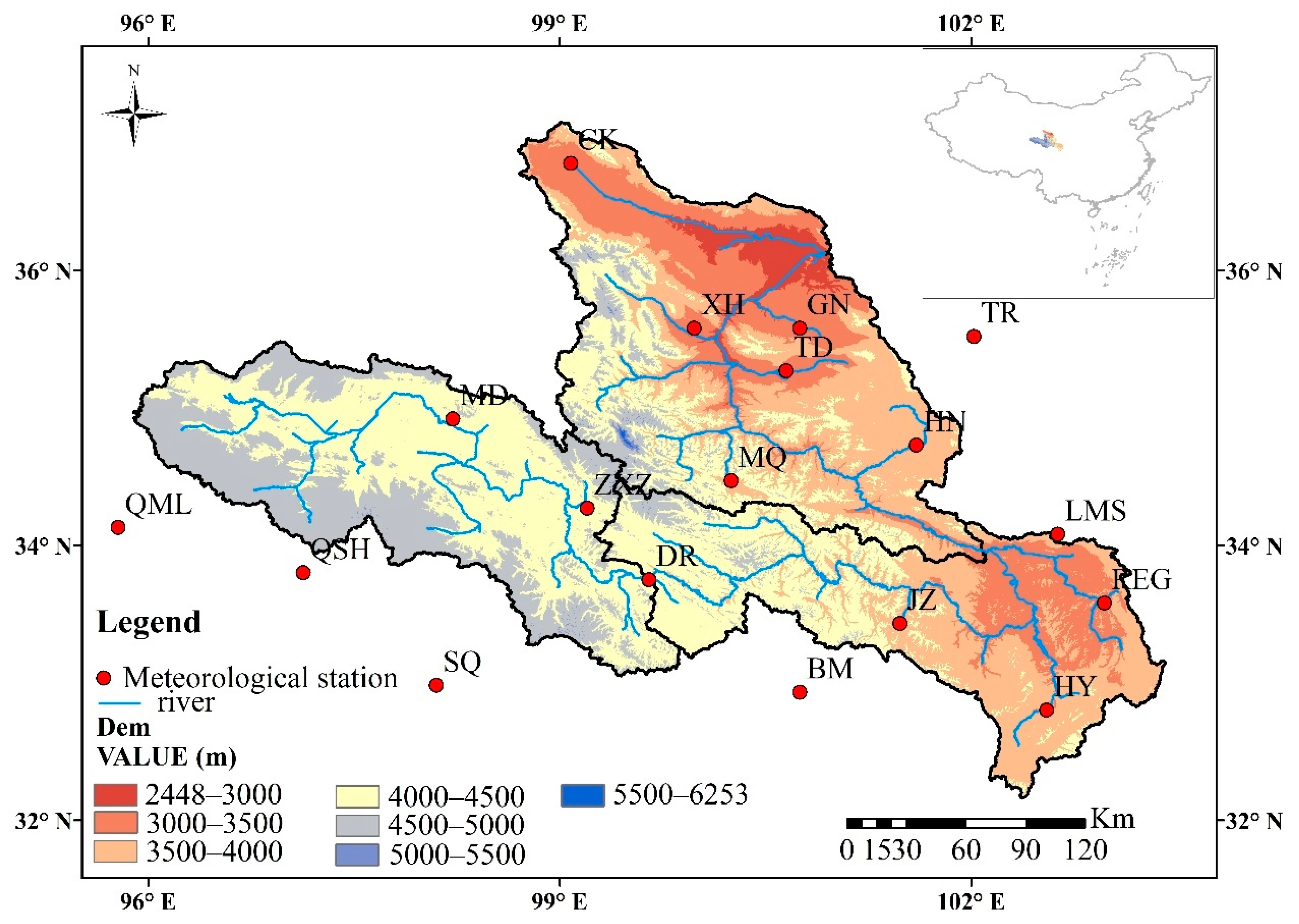
2.1. Study Region and Data Collection

The SRYE, generally defined as the Yellow River basin upstream of Longyangxia reservoir (Qinghai Province, China), is located in the northeast of the Qinghai-Tibet Plateau (32.5°–36.5° N and 95°–103.5° E). It covers 6 prefectures and 18 counties in Qinghai, Sichuan, and the Gansu Provinces, and is deployed with 18 meteorological stations (Figure 1), with a drainage area of 121,972 km². The region has a typical plateau continental climate, with alternate cold and hot seasons, as well as distinct dry and wet seasons, and has a long sunshine duration and strong radiation. The annual average temperature is −4.01 °C and the annual precipitation ranges from 350 to 750 mm, which decreases from the southeast to the northwest. Under the influence of monsoons, in summer and autumn (June to September) when precipitation is concentrated, southwest airflow from the Indian Ocean and warm–wet airflow from the Western Pacific are transported to the SRYE, forming weather with stable precipitation. The precipitation is distributed non-uniformly in time and space and changes largely interannually. The region is high altitude in the west and low altitude in the east, with an average altitude of 4500 m. The highest altitude is 6282 m (located in the Animaqing Mountain in the northwest of Maqin County, Guoluo Prefecture, Qinghai Province, China), and the lowest altitude is 2572 m (at the outlet of Longyangxia Reservoir).

The meteorological data used in this study include (1) data of monthly precipitation and monthly average temperature from 18 meteorological stations in the SRYE over 57 years (1960–2016). The data are from the China Meteorological Administration (http://data.cma.cn/, accessed on 5 July 2021) website, and data quality controls, including missing value inspections and extreme value tests, were strictly implemented. (2) Monthly data from 20 climate indexes, from 1960 to 2016, were downloaded from the website of Climate Prediction Center of the National Oceanic and Atmospheric Administration (NOAA) (http://www.esrl.noaa.gov/, accessed on 5 July 2021). (3) Dry-temperature profile observed from the COSMIC satellite (https://cdaac-www.cosmic.ucar.edu/, accessed on 5 July 2021).

The study shows that the spatial distribution and number of meteorological stations determine accuracy of the prediction model. When there are two few meteorological stations, the performance of the model will be extremely weakened, while too many meteorological stations will not improve the simulation accuracy indefinitely [33]. Therefore, this study removed data from meteorological stations with large deviations and selected meteorological stations distributed around the SRYE, as many as possible, to represent the overall precipitation of the SRYE. Precipitation from 1960 to 2016, from 18 meteorological stations in the SRYE, is closely related to altitude of the stations. With the increase of altitude, precipitation over the SRYE firstly increases and then decreases, overall.

2.2. Research Methods

2.2.1. Ensemble Empirical Mode Decomposition

Ensemble empirical mode decomposition (EEMD) is a new time-series signal processing method proposed by Wu and Huang to overcome the shortcomings of empirical mode decomposition (EMD) [34]. Thus, we implemented this method to extract the in-depth characteristics of the precipitation series. The process of EEMD is shown as follows:

(1) white noise series ${\beta }_i$(t) following normal distribution is added into the original signal x(t), that is,

$$x_i\left(t\right)=x\left(t\right)+{\beta }_i(t)$$

(1)

where, $x_i\left(t\right)$ represents the signal after adding white noise at i times.

(2) By decomposing $x_i\left(t\right)$ with EMD, the j intrinsic mode function (IMF) ${\mathrm{IMF}}_{ij}\left(t\right)$ and trend component $\mathrm{Re}{s}_i\left(t\right)$ are obtained.

(3) The ensemble averaging is performed for IMFs obtained from each decomposition, so that the added white noise offsets each other, thus obtaining the trend component $\mathrm{Re}s\left(t\right)$ extracted by EEMD.

$$\mathrm{Re}s(t)=\frac{1}{M}{\displaystyle \sum _{i=1}^M\mathrm{Re}{s}_i(t)}$$

(2)

The ${\mathrm{IMF}}_j\left(t\right)$ is shown as follows:

$${\mathrm{IMF}}_j(t)=\frac{1}{M}{\displaystyle \sum _{i=1}^M{\mathrm{IMF}}_{ij}(t)}$$

(3)

2.2.2. Extraction of Potential Energy of Gravity Waves

According to the linear theory of gravity waves, when only temperature is measured, the activity intensity of gravity waves can be characterized by potential energy [35]. The background temperature profile and temperature disturbance profile can be separated from the dry temperature profile at the COSMIC level 2. On this basis, the potential energy of gravity waves in the SRYE is calculated. The vertical interpolation, with a resolution of 200 m, is carried out in the range of 10–50 km for each profile at the monthly scale in the SRYE to eliminate temperature profiles exceeding the range of [−100, +10] °C. Through 3-sigma ($3\mathsf{\sigma }$) criteria, the data are preprocessed and the processed temperature profiles are averaged and subjected to a moving average, thus obtaining the background temperature profile $T_B$ of the SRYE. Afterward, the temperature disturbance profile T^′ can be obtained by subtracting the background temperature profile from the original temperature profile, and is detrended by quadratic fitting. By using a sixth-order Butterworth filter with a band-pass width of 2–10 km, other waves, except for gravity waves, are removed [36]. By substituting T^′ and $T_B$ into Formula (5), the potential energy of gravity waves is calculated.

The square of buoyancy frequency and potential energy of gravity waves are separately calculated through Formulas (4) and (5) [37].

$$N^2(z)=\frac{g}{T_B}(\frac{\partial T_B}{\partial Z}+\frac{g}{cp})$$

(4)

$$\mathrm{E}\mathrm{p}=\frac{1}{2}{(\frac{g}{N})}^2{(\frac{T^{\prime }}{T_B})}^2$$

(5)

where, $g=9.8 \mathrm{m}/{\mathrm{s}}^2 \mathrm{and} cp=1.005\times {10}^3 \mathrm{J}/\left(\mathrm{kg}·\mathrm{k}\right)$; z represents the height.

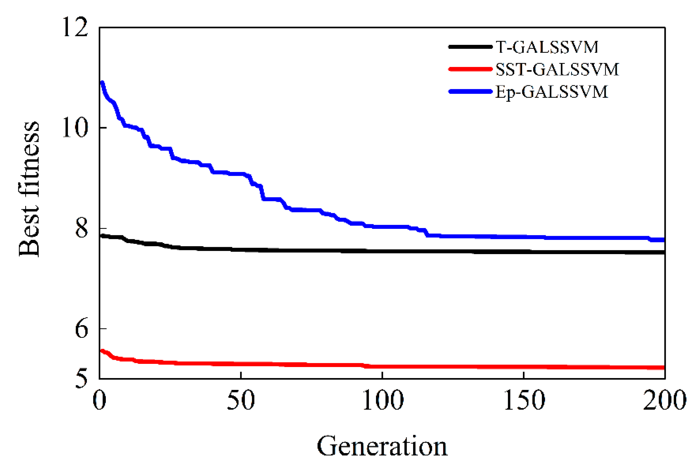
2.2.3. LSSVM Optimized by GA

The SVM, created by Vapnik [38], solves the problems that traditional methods may be trapped in local minimums and requires trial and error with experience; it has been applied in many fields. The LSSVM inherits the basic idea of SVM, replaces the inequality constraints of traditional SVM with equality constraints, and takes the quadratic term in the error as a loss function. It not only solves the problem that the number of hidden layer nodes is difficult to determine, but also has high accuracy and calculation speed.

For a training set $D=\left\{\left(x_{i,}{y}_i\right)|i=1,2,\dots ,n\right\},x\in R^d,y\in R$, the optimal decision-making function is constructed as follows [39]:

$$\mathrm{f}(x)={\omega }^T\phi \left(x\right)+b$$

(6)

where, ${\omega }^T$, $\phi \left(x\right)$ and b indicate the weight vector, linear mapping function and bias, respectively. The formula is transformed into the following regression and optimization problem for smooth approximation by using the structural risk minimization (SRM) criterion.

$$\underset{\omega ,b,e}{\min }J(\omega ,e)={\omega }^T\omega +\frac{1}{2}\gamma {\displaystyle \sum _{k=1}^N{e}_k^2}$$

(7)

$$y_k={\omega }^T\phi \left(x_k\right)+b+e_k$$

(8)

where, J, $\gamma$, and e represent the loss function, regularization parameter, and deviation, respectively. Based on the optimization theory, the Lagrange multiplier is introduced, so the Lagrange function of this problem is converted as follows:

$$L(\omega ,b,e,a)={\omega }^T\omega +\frac{1}{2}\gamma {\displaystyle \sum _{k=1}^N{e}_k^2}-{\displaystyle \sum _{k=1}^N{\alpha }_k}\left\{{\omega }^T\phi \left(x_k\right)+b+e_k-y_k\right\}$$

(9)

where, ${\alpha }_k$ denotes the Lagrange multiplier. Let each partial derivative be zero, the optimization conditions are shown as follows:

$$\frac{\partial L}{\partial \omega }=0\Rightarrow w={\displaystyle \sum _{k=1}^N{\alpha }_k\phi \left(x_k\right)}$$

(10)

$$\frac{\partial L}{\partial b}=0\Rightarrow {\displaystyle \sum _{k=1}^N{\alpha }_k=0}$$

(11)

$$\frac{\partial L}{\partial e_k}=0\Rightarrow {\alpha }_k=\gamma e_k$$

(12)

$$\frac{\partial L}{\partial {\alpha }_k}=0\Rightarrow \omega \cdot \phi (x_k)+b+e_k-y_k=0$$

(13)

By eliminating $e_k$ and $\omega$, the following linear equation set can be obtained.

$$\left[\begin{array}{cc}0& e_L^T\\ e_L& Q+I/Y\end{array}\right]\left[\begin{array}{c}b\\ \alpha \end{array}\right]=\left[\begin{array}{c}0\\ y\end{array}\right]$$

(14)

where, $y=y_1,\dots ,y_n{}^T,e_L=1,\dots ,1,\alpha ={\alpha }_1,\dots ,{\alpha }_N{}^T \mathrm{and} Q=\phi {\left(x_i\right)}^T\phi \left(x_i\right)$; I indicates the unit matrix. Let the kernel function be k($x_i,y_i$)$=\phi {\left(x_i\right)}^T\phi \left(x_i\right)$, a and b can be derived according to Formula (14), so LSSVM regression function is presented as follows:

$$f(x)=\hspace{0.17em}{\displaystyle \sum _{k=1}^N{\alpha }_{k}k\left(x,x_k\right)}+b$$

(15)

GA is a method to search the optimal solution by simulating the natural evolution process [40]. Therefore, this study used GA to optimize the kernel function γ and regularization parameter σ of the LSSVM, thus building the GA-LSSVM model. The radial basis function (RBF) that is widely used was selected as the kernel function. The maximum generation, population size and range of probability of crossover were 200, 20, and 0.7–0.9, respectively.

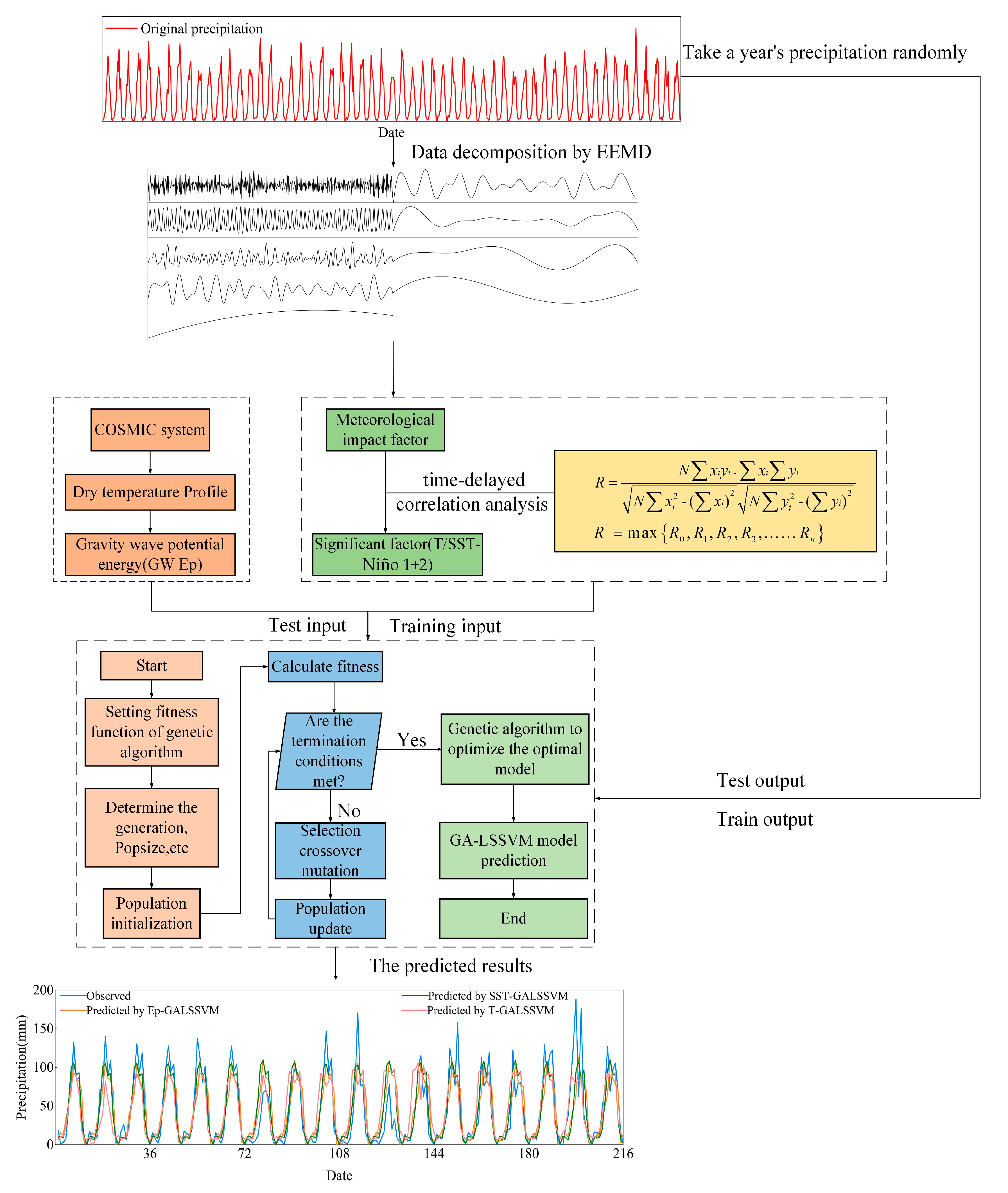
2.2.4. Establishment of the Prediction Model for Precipitation

This study built a basic data model based on monthly precipitation data in 2008 and geographic data of 18 meteorological stations in the SRYE. In order to carry out the simulation under the same standard, the meteorological stations were used as a test set, and the other 17 stations were used as a training set. On this basis, meteorological factors were integrated to seek the effects of driving factors on prediction results at each meteorological station. After repeated calculations, the results obtained by the algorithm did not change with the order of the training set. To establish the LSSVM model for the relationship between precipitation and each factor, it is necessary to select appropriate parameters γ and σ to set the model. However, these parameters are difficult to directly select. This study adopted GA for optimization and the specific steps are shown as follows:

• γ and σ are randomly generated.
• The LSSVM model is trained by the normalized training samples and the fitness function is used as the objective function of GA.
• The samples are separately trained and verified. The global optimal solution is searched and the output is through iteration.
• The LSSVM model is constructed by using the searched global optimal solution (γ, σ).

The prediction scheme for precipitation integrating meteorological factors is summarized in Figure 2.

Step 1: the monthly precipitation data from 18 stations (1960–2016) were subjected to mean processing. In the EEMD model, the amplitude of white noise was set to 0.2 times the standard deviation of the sample data, and the maximum number of sifting iterations was set to 200. Through EEMD on data, eight IMF components and one residual term were obtained, namely IMF1–IMF8, and r.

Step 2: the time-delayed correlation coefficients between 20 meteorological factors (1960–2016) and monthly precipitation series and their decomposed series were calculated and two maximum correlation coefficients were selected as the key factors affecting precipitation.

Step 3: potential energy of gravity waves extracted from the dry-temperature profile at COSMIC level 2 (2006–2014) was regarded as a significant topographic factor influencing precipitation.

Step 4: the LSSVM model was built and the optimal parameter was searched through GA. The selected two key factors and potential energy of gravity waves were taken as input variables of the model, while precipitation was used as output variable.

Step 5: to reveal the influences of each factor on precipitation, the precipitation from each meteorological station was predicted by taking 17 meteorological stations as a training set and one meteorological station as a test set.

Step 6: the accuracy of the model was evaluated by the mean absolute error (MAE), root mean square error (RMSE), and R², and the driving factors for precipitation were analyzed.

3. Results

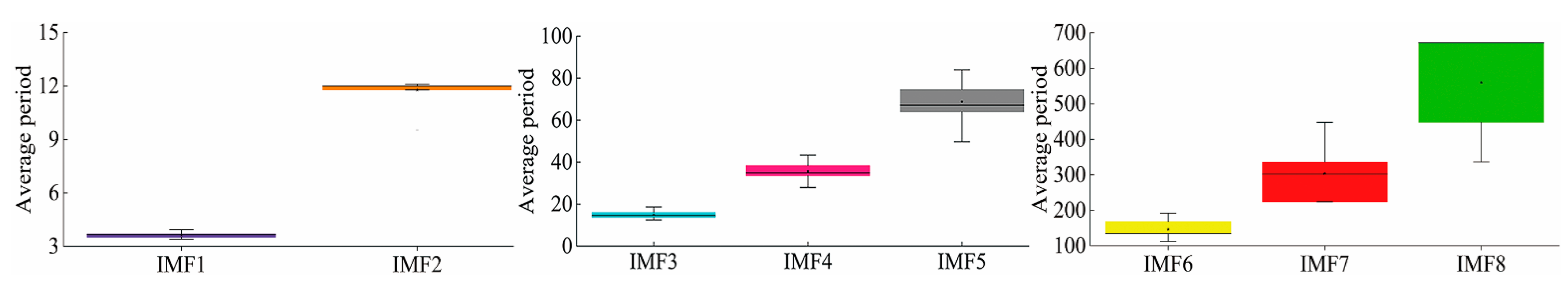
3.1. Analysis on Monthly Precipitation Series in Many Years Based on EEMD

The series of average precipitation in 1960–2016 and measured precipitation in 18 meteorological stations in the SRYE were decomposed, step-by-step, by using the EEMD method, obtaining eight IMFs, and one trend component (residue). To explore the average oscillation period of subseries at different time scales in the series of monthly precipitation, the average period of corresponding components was obtained by dividing the length of the series by the number of extreme points of each IMF component. As shown in Figure 3, at the monthly scale, the precipitation over the SRYE had a quasi-four-month (IMF1) climate variability. According to the statistics of IMF2–IMF6, precipitation presented a long period—an average period of quasi 12–134 months, showing an interannual variation of precipitation. The medians of the average periods of IMF7 and IMF8 are quasi-21 a and quasi-49 a, showing an interdecadal variation of precipitation. These IMFs include the periodic changes of external forcing of the climate system, as well as the nonlinear feedback effect of the climate system. Such periodic changes at different scales are not only affected by the multi-scale complex topography of the region, but also by the local atmospheric circulation system. These periods are the result of multiple influence factors.

3.2. Identification of Significant Meteorological Factors

To identify the significant correlation between monthly precipitation and meteorological factors in the SRYE, the time-delayed correlation analysis was conducted between each series of precipitation decomposed by EEMD and 20 meteorological factors; the 20 factors are shown in

Table 1. Abbreviations and full names of various indices.

Evaluation Indices
RMSE	Root Mean Square Error	R2	Coefficient of Determination
MAE	Mean Absolute Error
Meteorological Indices
Niño 1+2	Sea Surface Temperature (SST) in the Niño 1+2 region	STA	SST in the South Tropical Atlantic
Niño 3	SST in the Niño 3 region	AO	Arctic Oscillation
Niño 4	SST in the Niño 4 region	SOI	Southern Oscillation Index
Niño 3+4	SST in the Niño 3+4 region	PNA	Pacific-North America Index
NP	North Pacific Teleconnection	WP	Western Pacific Teleconnection
NAO	North Atlantic Oscillation	TNI	Trans Niño Index
ONI	Ocean Niño Index	TSA	Tropical South Atlantic Index
MEI	Multivariate ENSO Index	TNA	Tropical North Atlantic Index
NTA	SST in the Northern Tropical Atlantic	EAWR	East Atlantic Western Russia
PDO	Pacific Decadal Oscillation	WHWP	Western Hemisphere Warm Pool
Other Indices
Ep	Potential Energy of Gravity Waves	T	Temperature

. The delayed period was set as 0–11 months, and the two factors with the largest correlation coefficients were selected for each component.

Table 2. Meteorological factors with the highest correlation with the series of monthly precipitation and the EEMD decomposed series in the SRYE and correlation coefficients.

Component	Original Data		IMF1	IMF2	IMF3	IMF4
Time-delayed correlation coefficient (the first two largest)	T 0.887 (0)		NP 0.119 (9)	T 0.933 (0)	T 0.511 (0)	Niño 4 −0.305 (2)
	Niño 1+2 0.802 (4)		NAO 0.097 (9)	Niño 1+2 0.849 (4)	Niño 1+2 0.471 (4)	Niño 4 −0.302 (3)
Component		IMF5	IMF6	IMF7	IMF8	R
Time-delayed correlation coefficient (the first two largest)		ONI −0.228 (2)	NAO −0.194 (6)	NTA 0.122 (0)	NTA −0.331 (0)	NTA 0.552 (0)
		MEI 0.227 (1)	MEI −0.188 (1)	NTA −0.12 (1)	NTA −0.229 (1)	NTA 0.551 (1)

shows the two largest correlation coefficients between components at all stations in the SRYE and corresponding meteorological factors. The number following the correlation coefficient represents the delayed period. All correlation coefficients pass the significance test at the significant level of 1% (except the correlation coefficient of IMF1 and NAO). As demonstrated in Table 2, the correlation coefficient between temperature (T) of the original data and IMF2 and SST in the Niño 1+2 delayed for four months is the largest and passed the significance test at the level of 1%. This indicates that the precipitation in the SRYE is significantly affected by the SST in the Niño 1+2 index, delayed for four months, and temperature (T) in the same period at different time scales. Therefore, SST in the Niño 1+2 index and temperature (T) are the main meteorological factors affecting monthly precipitation in the SRYE.

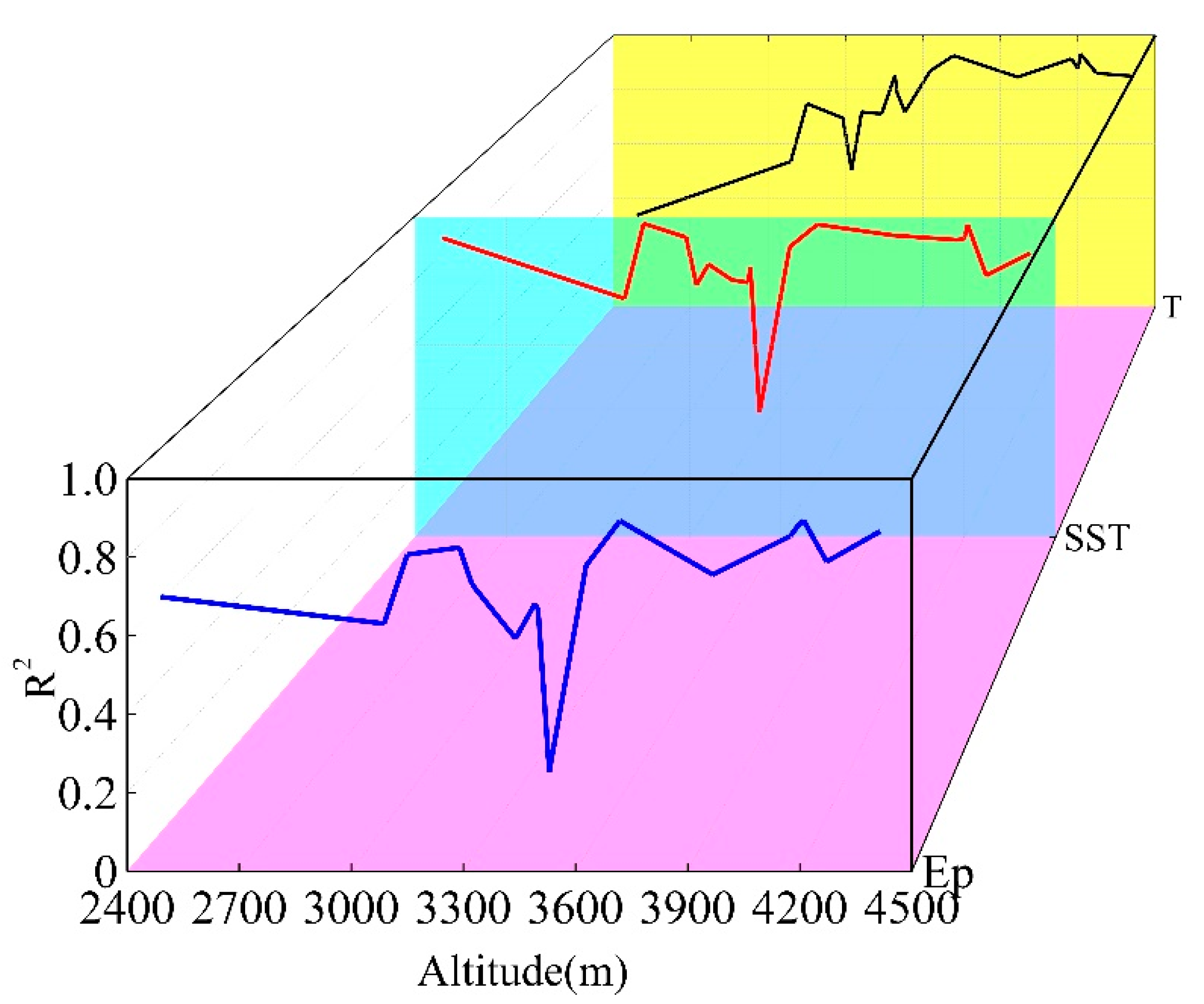
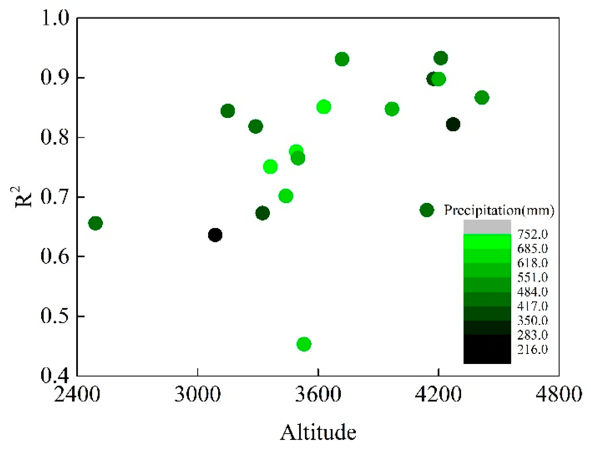
3.3. Analysis on the Correlation between Topographic Driving Factors and Precipitation

Gravity waves are excited by atmospheric convection and atmospheric motion in the Qinghai-Tibet Plateau [41]. In particular, gravity waves in the SRYE in the eastern part of the Qinghai-Tibet Plateau are more easily excited than in the western region. When gravity waves act, there is not (necessarily) a precipitation region, but there is usually at least one arc-shaped rain band or shower band before a wave trough comes. Not all gravity wave-induced events have a related precipitation system, but in the unstable atmosphere, gravity waves are one of the trigger mechanisms of rainstorms [42]. Since the gravity waves at an altitude of 17–24 km are mostly related to mountain waves [32], when processing the data of a gravity wave profile, the parts with elevations of 17–24 km on each profile are selected. The monthly variations of potential energy of gravity waves in the SRYE are obtained by averaging the potential energy of gravity waves at the elevation of 17–24 km after eliminating the value that the potential energy of gravity waves is too large (or smaller than zero). According to the calculation, the Pearson |r| between the potential energy of gravity waves and precipitation is 0.688, which shows a moderate correlation. In conclusion, the potential energy of gravity waves may have a certain correlation with precipitation. The weakest correlation is found between them, which is weaker than the correlations of SST in the Niño 1 + 2 region (r = 0.849) and surface temperature (r = 0.933) with precipitation.

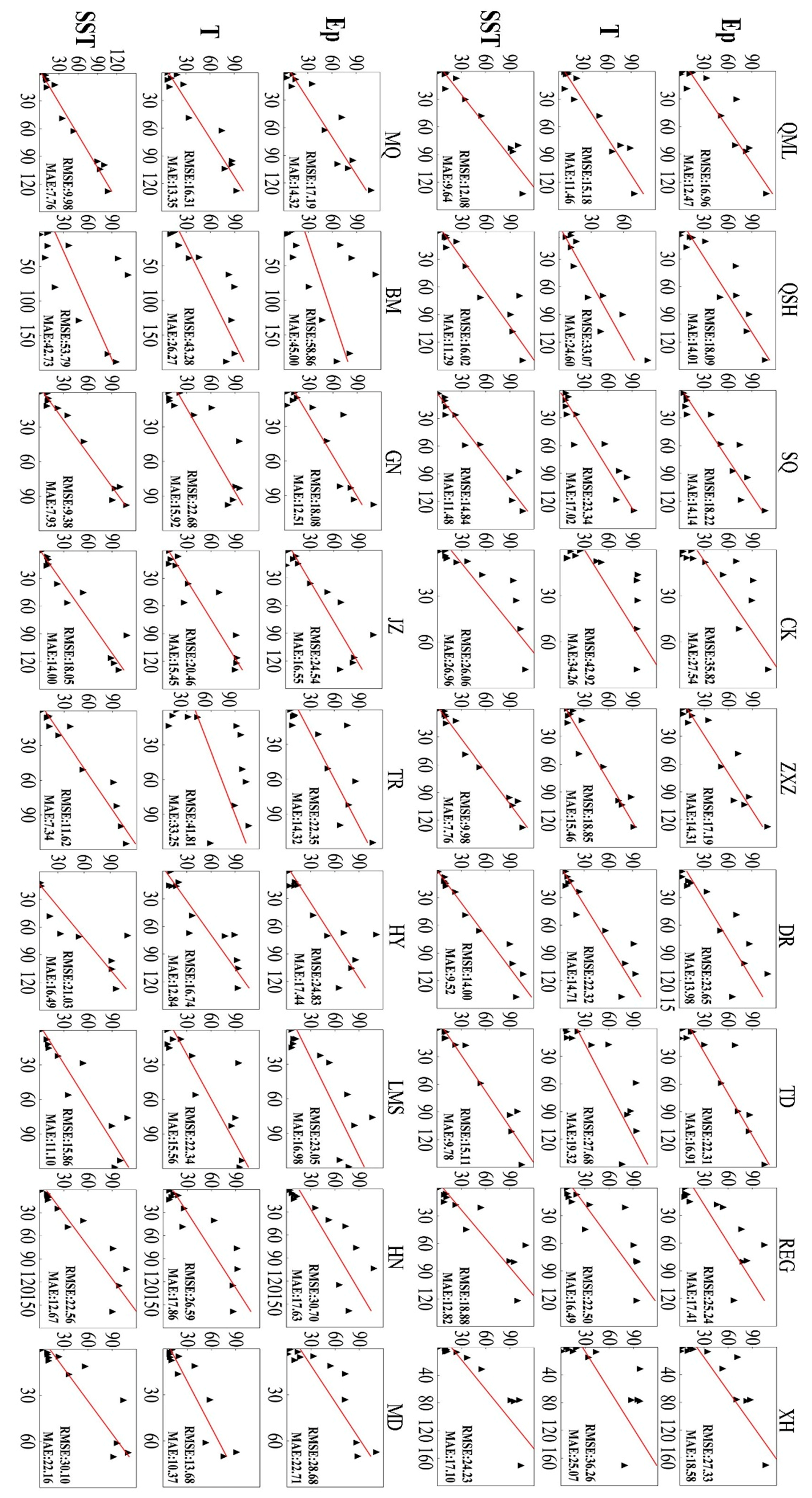
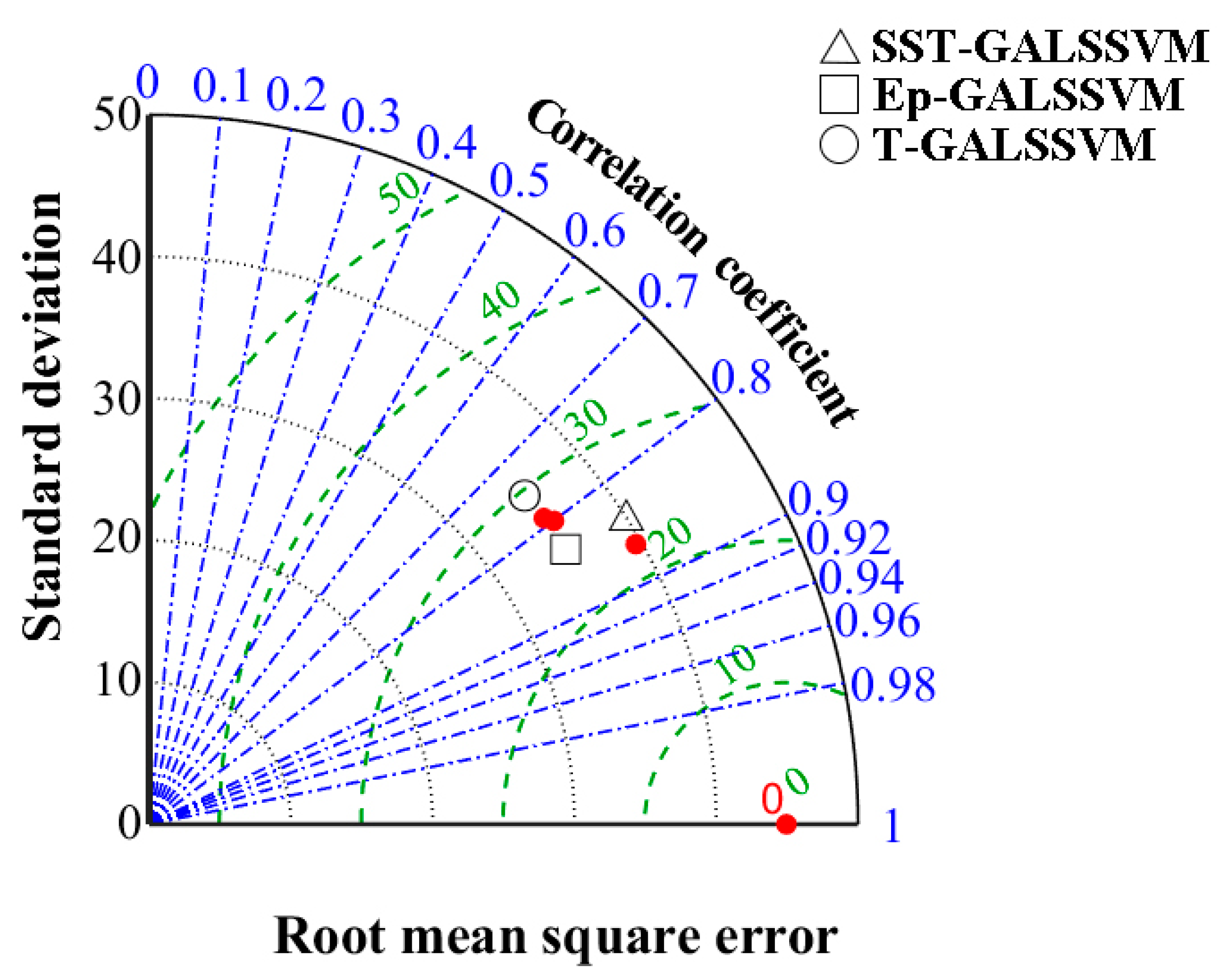
3.4. Analysis on Simulation Results of Precipitation

SST in the Niño 1+2 (Hereinafter referred to as SST), temperature (T), and potential energy of gravity waves (Ep) have strong correlations with precipitation in physical mechanisms and correlation analysis. For this reason, the above three highly correlated factors are integrated into the prediction model for precipitation to explore their influences on the accuracy of the model. The test results of the GA-LSSVM model are displayed in Figure 4. The horizontal and vertical axes separately represent the measured and predicted data. For Ep-GA-LSSVM, SST-GA-LSSVM, and T-GA-LSSVM, the ranges of RMSEs are 16.96–59.86 mm, 9.98–53.79 mm, and 15.18–43.28 mm, while those of MAEs are 12.47–45.00 mm, 7.76–42.43 mm, and 11.46–34.26 mm, respectively. The Ep-GA-LSSVM (R² = 0.254) and SST-GA-LSSVM (R² = 0.389) models exhibit the worst performance in BM Station in terms of the simulation results of long-term rainfall. For TR Station, T-GA-LSSVM model performs the worst in the prediction results (R² = 0.336), but Ep-GA-LSSVM (R² = 0.699) and SST-GA-LSSVM (R² = 0.933) models have high simulation accuracy. In the three models, the meteorological station with the highest test accuracy is the ZXZ station, with Ep-GA-LSSVM (R² = 0.893), SST-GA-LSSVM (R² = 0.975), and T-GA-LSSVM (R² = 0.931). According to statistics, 55% of the 54 prediction results show R² of the models above 80%.

Mirabbasi et al. [43] predicted monthly precipitations using the M5Tree model (MTM), multivariate adaptive regression spline (MARS), least square support vector regression (LSSVR), gene expressing programming (GEP), and artificial neural networks methods (ANNs). They used geographical information and rainfall data from 61 rain gauge stations in India. They divided the data into three sets, training, validation, and test. The test results show that for MTM, MARS, LSSVR, ANN, and GEP models, The RMSE ranges were 6.10–40.91 mm, 12.61–43.69 mm, 5.53–31.8 mm, 8.72–34.08 mm, and 26.07–58.91mm, respectively. The LSSVR model is better than other methods in the test stage. Kisi and Sanikhani [8] used adaptive neuro-fuzzy inference system (ANFIS), artificial neural networks (ANN), and support vector regression (SVR) models to predict long-term monthly precipitation in Iran. They found the lowest correlations as 0.696 (Sari station), 0.661 (Urmia station), and 0.785 (Bandar Lengeh station), and maximum correlations as 0.964 (Bam station), 0.944 (Fasa station), and 0.977 (Zabol and Tabas stations) for the ANFIS, SVM, and ANN models in the test stage, respectively. As can be seen from the above results, the applied models in this study provided relatively accurate results in modeling the precipitation of the SRYE.

The prediction indexes in each station are subjected to mean processing, and the results can be regarded as the simulation accuracy of precipitation over the whole SRYE. Overall, the accuracy grades of each model in long-term rainfall prediction are SST-GA-LSSVM (${\mathrm{R}}_{\mathrm{SST}}^2$ = 0.856, ${\mathrm{RMSE}}_{\mathrm{SST}}$ = 19.648, ${\mathrm{MAE}}_{\mathrm{SST}}$ = 14.363) > T-GA-LSSVM (${\mathrm{R}}_{\mathrm{T}}^2$ = 0.759, ${\mathrm{RMS}}_{\mathrm{ET}}$ = 25.889, ${\mathrm{MA}}_{\mathrm{ET}}$ = 18.848) ≈ Ep-GA-LSSVM (${\mathrm{R}}_{\mathrm{EP}}^2$ = 0.738, ${\mathrm{RMSE}}_{\mathrm{EP}}$ = 25.172, ${\mathrm{MAE}}_{\mathrm{EP}}$ = 18.156). Compared with other models, the SST-GA-LSSVM model is closer to the measured value.

The prediction results of the Ep-GA-LSSVM, SST-GA-LSSVM, and T-GA-LSSVM models for the test set in the SRYE are described in the form of the Taylor diagram (Figure 5). It can be seen that the prediction results of the SST-GA-LSSVM model are superior to those of the other two models, proving the superiority of the SST-GA-LSSVM model in precipitation prediction in the SRYE. The results obtained by the Ep-GA-LSSVM and T-GA-LSSVM models are similar. To be specific, compared with the SST-GA-LSSVM model, R² increases by 16%, while RMSE and MAE separately decrease by about 24% and 23% for the other two models.

3.5. Model Verification

In this research, the average curves of the best fitness and iterations of the GA-LSSVM model integrating three factors are shown in Figure 6. Each curve in the figure represents the optimization process under different conditions. It can be obtained that the optimal fitness of the three models obviously decreases and will not change after several evolutions, and the optimization results tend to converge. When the Ep-GA-LSSVM model evolves to the 120th generation, the optimal fitness function for optimization results gradually tends to be stable, at about 7.8, indicating that individuals are found near the optimal solution. The values of the optimal fitness functions of the T-GA-LSSVM and SST-GA-LSSVM models gradually stabilize at about 7.8 and 5.6 after 45 and 90 generations. When GA is used for optimization and training, the smaller the optimal fitness of individuals is, the higher the prediction accuracy. This suggests that the SST-GA-LSSVM model is better than the other two models in optimizing network parameters.

4. Discussions

There is an obvious non-linear relationship between precipitation and altitude, but few people have studied the relationship between precipitation prediction accuracy and altitude. Data-driven methods can be used to reasonably evaluate the information behind the data. Therefore, this study drew the schematic diagram for the relationship between the elevation of meteorological stations and prediction accuracy R² of each model (Figure 7). After integrating T, the prediction accuracy is improved most significantly. The accuracy of the prediction model for precipitation, integrating the three driving factors, increases with elevation overall. However, the prediction accuracy at the altitude of 3500 m does not confirm the overall trend. Such a law is reflected in the results of the three simulation methods. As shown in the figure, such a phenomenon may be correlated with distribution laws of precipitation with vertical gradients in this region.

To reveal the possible relationship between precipitation and prediction accuracy of the model, this study established a scatter diagram for the relationship of precipitation with altitude and accuracy, R². The relationship between precipitation and altitude of meteorological stations in the study area is shown in Figure 8. It can be observed that the regions with abundant precipitation (average annual precipitation > 600 mm) are concentrated near the altitude of 3500 m, where the prediction accuracy of precipitation is at a low level ($\overline{{\mathrm{R}}^2}=0.70$). The regions with less precipitation (average annual precipitation < 400 mm) are concentrated in high- and low-altitude regions, which is consistent with the regions with abundant precipitation, showing low prediction accuracy ($\overline{{\mathrm{R}}^2}=0.71$). However, the prediction accuracy is higher in the regions where the annual average precipitation is more than 400 mm and less than 600 mm ($\overline{{\mathrm{R}}^2}=0.86$). Therefore, compared with the regions with high and low annual average precipitation, this study has a better applicability to the SRYE with moderate precipitation.

5. Conclusions

By integrating meteorological factors selected by EEMD and the potential energy of gravity waves representing topographic factors in the SRYE into the GA-LSSVM model for precipitation prediction, this study discussed the prediction effects of different factors in the estimation of long-term precipitation. The results demonstrate that the SST-GA-LSSVM model is the optimal model (${\mathrm{R}}_{\mathrm{SST}}^2$ = 0.856, ${\mathrm{RMSE}}_{\mathrm{SST}}$ = 19.648, ${\mathrm{MAE}}_{\mathrm{SST}}$ = 14.363) in the test stage and the simulation results of the Ep-GA-LSSVM model are similar to those of the T-GA-LSSVM model. From the perspectives of RMSE and MAE, in terms of accuracy, the SST-GA-LSSVM model improves by 24% and 23% compared with the other two models. According to the statistics of prediction results, R² of the three models, more than a half of meteorological stations exhibit R² over 80%.

Furthermore, this research analyzed the possible relationship of prediction accuracy R² of the model with altitude and annual average precipitation. The accuracy is sensitive to influences of altitude and accurate prediction results are easily obtained at high altitude. The SST-GA-LSSVM model can “fill the gap” of low prediction accuracy of other models at low altitudes. Using the altitude of 3500 m as the boundary, the prediction accuracy R² in the region with annual precipitation of 400–600 mm is about 10% higher than that in the regions with different precipitation.

In conclusion, this study proposes a prediction model for precipitation, combined with physical mechanisms, while being independent of historical precipitation data in the field of precipitation prediction. By integrating key factors driving precipitation, this study achieved high accuracy of prediction results, which is conducive toward understanding precipitation prediction. The relevant research results are favorable for flood prevention and risk management of water resources. It is worth noting that the framework and methods in this study can be popularized to regions without data.

References

1. Quan, Q.; Hao, Z.; Xifeng, H.; Jingchun, L. Research on water temperature prediction based on improved support vector regression. Neural Comput. Appl. 2020, 1–10. [Google Scholar] [CrossRef]
2. Feng, Z.; Niu, W.; Tang, Z.; Jiang, Z.; Xu, Y.; Liu, Y.; Zhang, H. Monthly runoff time series prediction by variational mode decomposition and support vector machine based on quantum-behaved particle swarm optimization. J. Hydrol. 2020, 583, 124627. [Google Scholar] [CrossRef]
3. Yoon, H.; Jun, S.-C.; Hyun, Y.; Bae, G.-O.; Lee, K.-K. A comparative study of artificial neural networks and support vector machines for predicting groundwater levels in a coastal aquifer. J. Hydrol. 2011, 396, 128–138. [Google Scholar] [CrossRef]
4. Abdulelah Al-Sudani, Z.; Salih, S.Q.; Sharafati, A.; Yaseen, Z.M. Development of multivariate adaptive regression spline integrated with differential evolution model for streamflow simulation. J. Hydrol. 2019, 573, 1–12. [Google Scholar] [CrossRef]
5. Kisi, O. Modeling reference evapotranspiration using three different heuristic regression approaches. Agric. Water Manag. 2016, 169, 162–172. [Google Scholar] [CrossRef]
6. Mouatadid, S.; Adamowski, J.F.; Tiwari, M.K.; Quilty, J.M. Coupling the maximum overlap discrete wavelet transform and long short-term memory networks for irrigation flow forecasting. Agric. Water Manag. 2019, 219, 72–85. [Google Scholar] [CrossRef]
7. Kumar, D.; Pandey, A.; Sharma, N.; Flügel, W.-A. Daily suspended sediment simulation using machine learning approach. CATENA 2016, 138, 77–90. [Google Scholar] [CrossRef]
8. Kisi, O.; Sanikhani, H. Prediction of long-term monthly precipitation using several soft computing methods without climatic data. Int. J. Climatol. 2015, 35, 4139–4150. [Google Scholar] [CrossRef]
9. Liu, X.; Bo, L.; Luo, H. Bearing faults diagnostics based on hybrid LS-SVM and EMD method. Measurement 2015, 59, 145–166. [Google Scholar] [CrossRef]
10. Chisola, M.N.; van der Laan, M.; Bristow, K.L. A landscape hydrology approach to inform sustainable water resource management under a changing environment. A case study for the Kaleya River Catchment, Zambia. J. Hydrol. Reg. Stud. 2020, 32, 100762. [Google Scholar] [CrossRef]
11. Safari, M.J.S.; Mohammadi, B.; Kargar, K. Invasive weed optimization-based adaptive neuro-fuzzy inference system hybrid model for sediment transport with a bed deposit. J. Clean. Prod. 2020, 276, 124267. [Google Scholar] [CrossRef]
12. Ahmed, K.; Sachindra, D.A.; Shahid, S.; Iqbal, Z.; Nawaz, N.; Khan, N. Multi-model ensemble predictions of precipitation and temperature using machine learning algorithms. Atmos. Res. 2020, 236, 104806. [Google Scholar] [CrossRef]
13. Chang, F.-J.; Liang, J.-M.; Chen, Y.-C. Flood forecasting using radial basis function neural networks. Syst. Man Cybern. Part C Appl. Rev. IEEE Trans. 2001, 31, 530–535. [Google Scholar] [CrossRef]
14. Yang, T.; Liu, J.; Chen, Q. Assessment of plain river ecosystem function based on improved gray system model and analytic hierarchy process for the Fuyang River, Haihe River Basin, China. Ecol. Modell. 2013, 268, 37–47. [Google Scholar] [CrossRef]
15. Zheng, H.; Chen, L.; Han, X.; Zhao, X.; Ma, Y. Classification and regression tree (CART) for analysis of soybean yield variability among fields in Northeast China: The importance of phosphorus application rates under drought conditions. Agric. Ecosyst. Environ. 2009, 132, 98–105. [Google Scholar] [CrossRef]
16. de Lavôr Paes Barreto, M.; Netto, A.M.; da Silva, J.P.S.; Amaral, A.; Borges, E.; de França, E.J.; Vale, R.L. Gray water footprint assessment for pesticide mixtures applied to a sugarcane crop in Brazil: A comparison between two models. J. Clean. Prod. 2020, 276, 124254. [Google Scholar] [CrossRef]
17. Wang, L.; Xie, Y.; Wang, X.; Xu, J.; Zhang, H.; Yu, J.; Sun, Q.; Zhao, Z. Meteorological sequence prediction based on multivariate space-time auto regression model and fractional calculus grey model. Chaos Solitons Fractals 2019, 128, 203–209. [Google Scholar] [CrossRef]
18. Corchado, J.M.; Lees, B. A hybrid case-based model for forecasting. Appl. Artif. Intell. 2001, 15, 105–127. [Google Scholar] [CrossRef]
19. Liang, J.; Li, W.; Bradford, S.A.; Šimůnek, J. Physics-Informed Data-Driven Models to Predict Surface Runoff Water Quantity and Quality in Agricultural Fields. Water 2019, 11, 200. [Google Scholar] [CrossRef] [Green Version]
20. Qian, K.; Mohamed, A.; Claudel, C. Physics Informed Data Driven Model for Flood Prediction: Application of Deep Learning in Prediction of Urban Flood Development. arXiv 2019, arXiv:1908.10312. Available online: https://arxiv.org/abs/1908.10312 (accessed on 20 August 2021).
21. Liu, G.; Wu, R. Spatial and temporal characteristics of summer precipitation events spanning different numbers of days over Asia. J. Climatol. 2016, 36, 2288–2302. [Google Scholar] [CrossRef]
22. Sohn, B.J.; Yeh, S.W.; Lee, A.; Lau, W.K.M. Regulation of atmospheric circulation controlling the tropical Pacific precipitation change in response to CO2 increases. Nat. Commun. 2019, 10, 1108. [Google Scholar] [CrossRef] [Green Version]
23. Vecchi, G.A.; Soden, B.J.J. Global Warming and the Weakening of the Tropical Circulation. J. Clim. 2007, 20, 4316–4340. [Google Scholar] [CrossRef] [Green Version]
24. Aizen, E.M.; Aizen, V.B.; Melack, J.M.; Nakamura, T.; Ohta, T. Precipitation and atmospheric circulation patterns at mid-latitudes of Asia. Int. J. Climatol. 2001, 21, 535–556. [Google Scholar] [CrossRef]
25. Prein, A.F.; Gobiet, A.; Truhetz, H.; Keuler, K.; Goergen, K.; Teichmann, C.; Fox Maule, C.; van Meijgaard, E.; Déqué, M.; Nikulin, G.; et al. Precipitation in the EURO-CORDEX 0.11° and 0.44° simulations: High resolution, high benefits? Clim. Dyn. 2016, 46, 383–412. [Google Scholar] [CrossRef] [Green Version]
26. Cox, J.; Steenburgh, W.; Kingsmill, D.; Shafer, J.; Colle, B.; Bousquet, O.; Smull, B.; Cai, H. The kinematic structure of a Wasatch Mountain winter storm during IPEX IOP3. Mon. Weather Rev.-MON Weather REV 2005, 133, 521–542. [Google Scholar] [CrossRef]
27. Lorente-Plazas, R.; Mitchell, T.; Mauger, G.; Salathé, E. Local Enhancement of Extreme Precipitation during Atmospheric Rivers as Simulated in a Regional Climate Model. J. Hydrometeorol. 2018, 19, 1429–1446. [Google Scholar] [CrossRef]
28. James, C.N.; Houze, R.A. Modification of precipitation by coastal orography in storms crossing northern California. Mon. Weather Rev. 2005, 133, 3110–3131. [Google Scholar] [CrossRef]
29. Colle, B.A.; Wolfe, J.B.; Steenburgh, W.J.; Kingsmill, D.E.; Cox, J.A.W.; Shafer, J.C. High-resolution simulations and microphysical validation of an orographic precipitation event over the Wasatch Mountains during IPEX IOP3. Mon. Weather Rev. 2005, 133, 2947–2971. [Google Scholar] [CrossRef] [Green Version]
30. Neiman, P.; Ralph, F.; White, A.; Kingsmill, D.; Persson, O. The Statistical Relationship between Upslope Flow and Rainfall in California’s Coastal Mountains: Observations during CALJET. Mon. Weather Rev.-MON Weather REV 2002, 130, 1468–1492. [Google Scholar] [CrossRef]
31. Lin, Y.-L.; Chiao, S.; Wang, T.-A.; Kaplan, M.; Weglarz, R. Some Common Ingredients for Heavy Orographic Rainfall. Weather Forecast.-Weather Forecast 2001, 16, 633–660. [Google Scholar] [CrossRef]
32. Khan, A.; Jin, S. Gravity wave activities in Tibet observed by COSMIC GPS radio occultation. Geod. Geodyn. 2018, 9, 504–511. [Google Scholar] [CrossRef]
33. Bárdossy, A.; Das, T. Influence of rainfall observation network on model calibration and application. Hydrol. Earth Syst. Sci. 2008, 12, 77–89. [Google Scholar] [CrossRef] [Green Version]
34. Wu, Z.; Huang, N. Ensemble Empirical Mode Decomposition: A Noise-Assisted Data Analysis Method. Adv. Adapt. Data Anal. 2009, 1, 1–41. [Google Scholar] [CrossRef]
35. Liang, C.; Xue, X.; Chen, T.-D. An investigation of the global morphology of stratosphere gravity waves based on COSMIC observations. Chin. J. Geophys. Acta Geophys. Sin. 2014, 57, 3668–3678. [Google Scholar] [CrossRef]
36. Tsuda, T.; Nishida, M.; Rocken, C.; Ware, R. A Global Morphology of Gravity Wave Activity in the Stratosphere Revealed by the GPS Occultation Data (GPS/MET). J. Geophys. Res. 2000, 105, 7257–7274. [Google Scholar] [CrossRef]
37. Yang, S.-S.; Pan, C.J.; Das, U.; Lai, H.C. Analysis of synoptic scale controlling factors in the distribution of gravity wave potential energy. J. Atmos. Solar-Terr. Phys. 2015, 135, 126–135. [Google Scholar] [CrossRef]
38. Cortes, C.; Vapnik, V. Support-vector networks. Mach. Learn. 1995, 20, 273–297. [Google Scholar] [CrossRef]
39. Pan, X.; Xing, Z.; Tian, C.; Wang, H.; Liu, H. A method based on GA-LSSVM for COP prediction and load regulation in the water chiller system. Energy Build. 2021, 230, 110604. [Google Scholar] [CrossRef]
40. Chen, L.; Mcphee, J.; Yeh, W. A Diversified Multiobjective GA for Optimizing Reservoir Rule Curves. Adv. Water Resour. 2007, 30, 1082–1093. [Google Scholar] [CrossRef]
41. Hoffmann, L.; Xue, X.; Alexander, M.J. A global view of stratospheric gravity wave hotspots located with atmospheric infrared sounder observations. J. Geophys. Res. Atmos. 2013, 118, 416–434. [Google Scholar] [CrossRef] [Green Version]
42. Li, M. Studies on the gravity wave initiation of the excessively heavy rainfall. Chin. J. Atmos. Sci. 1978, 2, 201–209. [Google Scholar] [CrossRef]
43. Mirabbasi, R.; Kisi, O.; Sanikhani, H.; Gajbhiye Meshram, S. Monthly long-term rainfall estimation in Central India using M5Tree, MARS, LSSVR, ANN and GEP models. Neural Comput. Appl. 2019, 31, 6843–6862. [Google Scholar] [CrossRef]
Figure 1. Location of the SRYE and the meteorological stations.
Atmosphere 12 01076 g001
Figure 2. Prediction scheme for precipitation combining with meteorological factors.
Atmosphere 12 01076 g002
Figure 3. Boxplot of average periods of IMFs in the series of monthly precipitation in 18 meteorological stations.
Atmosphere 12 01076 g003
Figure 4. Prediction results of precipitation integrating SST, T, and Ep.
Atmosphere 12 01076 g004
Figure 5. Taylor diagram of precipitation prediction integrating meteorological factors. The blue contours represent Pearson’s correlation coefficient; the green contours indicate RMSE; the black contours denote standard deviation of simulated diagram.
Atmosphere 12 01076 g005
Figure 6. Parameter optimization based on GA.
Atmosphere 12 01076 g006
Figure 7. The relationship between prediction accuracy R2 of the model integrating factors and altitude. The blue, red, and black polylines represent the factors Ep, SST, and T, respectively.
Atmosphere 12 01076 g007
Figure 8. Scatter diagram for the relationship of precipitation with altitude and prediction accuracy R2.
Atmosphere 12 01076 g008