Article

Enhancing the Output of Climate Models: A Weather Generator for Climate Change Impact Studies

Department of Civil and Industrial Engineering-Structural Division, University of Pisa, Largo Lucio Lazzarino 1, 56122 Pisa, Italy
*
Author to whom correspondence should be addressed.
Atmosphere 2021, 12(8), 1074; https://doi.org/10.3390/atmos12081074
Submission received: 31 July 2021 / Revised: 17 August 2021 / Accepted: 18 August 2021 / Published: 21 August 2021
(This article belongs to the Topic Climate Change and Environmental Sustainability)

Abstract

:
Evaluation of effects of climate change on climate variable extremes is a key topic in civil and structural engineering, strongly affecting adaptation strategy for resilience. Appropriate procedures to assess the evolution over time of climatic actions are needed to deal with the inherent uncertainty of climate projections, also in view of providing more sound and robust predictions at the local scale. In this paper, an ad hoc weather generator is presented that is able to provide a quantification of climate model inherent uncertainties. Similar to other weather generators, the proposed algorithm allows the virtualization of the climatic data projection process, overcoming the usual limitations due to the restricted number of available climate model runs, requiring huge computational time. However, differently from other weather generation procedures, this new tool directly samples from the output of Regional Climate Models (RCMs), avoiding the introduction of additional hypotheses about the stochastic properties of the distributions of climate variables. Analyzing the ensemble of so-generated series, future changes of climatic actions can be assessed, and the associated uncertainties duly estimated, as a function of considered greenhouse gases emission scenarios. The efficiency of the proposed weather generator is discussed evaluating performance metrics and referring to a relevant case study: the evaluation of extremes of minimum and maximum temperature, precipitation, and ground snow load in a central Eastern region of Italy, which is part of the Mediterranean climatic zone. Starting from the model ensemble of six RCMs, factors of change uncertainty maps for the investigated region are derived concerning extreme daily temperatures, daily precipitation, and ground snow loads, underlying the potentialities of the proposed approach.

1. Introduction

Climate change is becoming more and more relevant in many sciences and engineering disciplines, including civil and structural engineering. Thus, its implications and potential future risks are increasingly debated [1,2,3,4]. The potential increase in frequency and intensity of natural hazards significantly influences not only the design and the service level of new structures and infrastructures but also the structural safety and the assessment of existing ones, with relevant consequences in terms of direct and indirect costs [5], and in planning of maintenance or strengthening interventions [4,6,7,8]. It must be remarked that especially for critical infrastructures, huge indirect costs can derive from the increase of out of service time [9,10]. In assessing the influences of climate changes on the performances of engineering works, attention should be devoted both to the peculiarities of the investigated structures and to the objectives of the study. In fact, while in many works, the most pertinent information is the evolution over time of the mean value of the relevant climatic variables [11], in other works, the focus is on the extremes [5]. A number of cases are typically governed by mean values: for example, estimates of electrical power productivity of wind turbines [12] or hydroelectric power plants [13], assessment of navigability of rivers and channels [14], evaluation of water table level, availability of fresh water resources [15], estimation of sea level rise [11], agricultural and zootechnics production [16], and deterioration effects on structures and finishes [17,18]. Other cases are mainly governed by extreme values: for example, design of civil engineering and geotechnical works [4,6,7,8], assessment of minimum vital outflow of rivers and torrents, structural design of wind turbines [19], evaluation of minimum height of embankments [20], out of service time of navigable channels [14], icing effects on cables and electrical power lines [21,22], flooding [23], and scour of bridge piles [4].
In modern codes, such as the Eurocodes [24,25,26,27], design values of effects of climatic variables, snow and rain precipitations, shade air temperature, wind velocity, etc., are evaluated starting from the so-called representative values of climatic variables themselves, which are characterized by a given probability of exceedance, p , in a reference time interval [24,28]. In the Eurocodes [24,25,26,27], four main representative values are usually defined [24]:
  • The characteristic value, for which p = 2 % in one year;
  • The combination value, leading, together with the characteristic value of another variable action of different nature, to a combined effect characterized by p = 2 % in one year;
  • The frequent value, roughly exceeded from 100 to 300 times in one year;
  • The quasi permanent value, exceeded for more than 50% of the design working life of the construction.
Assuming suitable extreme value distributions, the aforementioned representative values are commonly evaluated under the hypothesis of climate being stationary over time [4,29]. As this assumption is clearly violated when climate change effects occur, relevant assessment of representative values should duly take into account non-stationarity, also in view of the definition of suitable adaptation strategies for the design of resilient buildings and infrastructures [30,31].
The evolution over time of climatic variables and climatic actions is usually assessed on the basis of the outputs of General (or Global) Climate Models (GCMs) or Regional Climate Models (RCMs). In comparison with GCMs, the RCMs are associated to more refined grid resolution, typically ranging from 10 to 20 km, so allowing more detailed local estimates. In any case, owing to the complexity of the problem and the computational time needed for a single run (simulation), independently on the scale of the model, i.e., the typical dimensions of individual cells, the number of reliable climatic models and the total number of available runs are so limited that further elaborations are needed, aiming to increase the representativeness of the outcomes of climate models. A promising method to enhance the significance of the outputs of the climate models is based on the implementation of suitable weather generators. The basic idea of the method is the artificial generation of additional outputs of climatic models, via random extraction of daily values of relevant climatic variables from appropriate homogenous populations of climatic variables, whose statistical properties are suitably assessed from the available runs of various climatic models. In this way, it is also possible to evaluate model uncertainties due to the inherent climate variability, which is fundamental information for the interpretation of climate projection, especially at smaller scales [32]. Weather generators, which have been proposed and largely developed in the water and hydraulic engineering field [33], are nowadays largely adopted for statistical downscaling in climate change investigations [34,35,36,37].
Evidently, the assembly of the homogenous populations to be randomly sampled is the core of the procedure, potentially impacting the outcomes. More specifically, assumptions about the probabilistic description of such populations determine post-sample resulting populations complying with the starting hypotheses, so that uncertainties associated with probabilistic models cannot be directly considered. To overcome this issue, a novel weather generation technique is proposed, making direct use of the outputs of climate models. The proposed procedure is particularly suitable for studying the evolution of climatic variables over time as a function of climate change, starting from the output of Regional Climate Models (RCMs). The procedure allows evaluating the dependence of climate projections on most relevant sources of uncertainty, i.e., emission scenarios, climate models, and internal variability [38].
Nonparametric resampling techniques were already proposed for generating daily temperature and precipitation from historical data [39,40]. In these methods, resampling was carried out considering the nearest neighbors for the simulated day in terms of a weighted Euclidean distance [39] or conditioning on indices of atmospheric circulation [40].
In the present study, the generation is elaborated on the basis of climate model outputs according to an original and simplified procedure, with the aim of reproducing the internal variability of climate model runs, in such a way to estimate the uncertainty in the expected changes of climate statistics.
The efficiency and performances of the proposed weather generator are demonstrated discussing a relevant case study: the variation over time, until the year 2100, of characteristic values of significant climatic actions, daily maximum and minimum temperature, precipitations, and ground snow load, in the central Eastern part of Italy, which is located in the Mediterranean climatic area. In the study, the weather generated series are analyzed in terms of factor of changes (FC) [41], described in the following section, which are a very effective way to describe the relative variations of the considered variable.
The aim of the case study is to illustrate the suitability of the proposed methodology for the treatment of climate model outputs and is not intended to provide detailed guidance for adaptation strategies in the field of climatic actions on structures. In fact, a discussion is currently ongoing on the use of IPCC baseline scenarios, which are central to climate science and adaptation policy [42]. Scenarios are affected by deep uncertainties that are inherent in assumptions about significant factors: future technology developments, lifestyle changes, policy formulations, economic and demographic trends, and so on [43]. Notwithstanding this deep uncertainty, no equal probabilities are generally assigned by expert to the total range of future emissions. A discussion about this relevant issue can be found in [43]. In the present study, to assess the potentialities of the method, a sensitivity analysis is performed considering two possible scenarios belonging to the Representative Concentration Pathways (RCPs) set [44]: RCP4.5 and RCP8.5. Of course, the definition of the most “realistic” RCP is out of the scope of the present work.

2. Methodology

2.1. Weather Generators

As already mentioned, stochastic weather generators are suitable random extraction algorithms for the automatic generation of time-series of climatic variables. The main feature of these algorithms is their ability to generate day-by-day data series of climatic variables, starting from suitable populations of input data, based on observations, if any, and projections provided by climate models. Of course, weather generators cannot be confused with weather prediction algorithms: in fact, while weather projections are based on numerical methods for the solution of the physical equations describing the earth climate and its dependency on time, weather generators are implements for the origination of additional and virtual time-dependent results or forecasts, based on synthetic representations of available information, regardless of whether the information itself is obtained from observation or simulations [34].
Weather generators were firstly proposed and applied for risk assessment purposes in hydrological and agricultural fields [33,45]. Their main intended use was the simulation of series of climatic data sufficiently extended over time, allowing to fill the lack of reliable meteorological data, and to extend the available information to unmonitored sites, by resorting to artificial measurements. More recently, the field of application of weather generators has been considerably enlarged. In fact, starting from the outputs of individual runs of the climate models and taking into account the relevant statistical parameters of each climatic variable, they are more and more adopted to obtain supplementary virtual runs of the models. Although a sensible difference is still present between the predictions of regional climate models and local observations [46], weather generators can be very useful tools to enhance the climate projections and to achieve more sound information about the influence of climate changes. More precisely, once the evolution of the governing climatic parameters is derived from the climate model outputs, site-specific climate change scenarios can be assessed applying suitable weather generation algorithms. Truly, distinctive features of weather generators are much wider: for example, they can be efficiently applied to evaluate how the uncertainties on the projections of effects of climate change influence climate variable statistics and calculate the prediction intervals associated with the available climate model outputs. To obtain this information, two different approaches can be envisaged, depending on the way the changes over time are described: the variations over time of featuring statistical parameters of relevant climatic variables can be studied considering trends in the weather series, or, alternatively, by means of the already recalled factor of change approach, considering the variations of the statistical properties of the climate variables. The latter approach is based on the assumption, corroborated by numerical and experimental evidence, that influences of climate change are more soundly evaluated considering the variation of statistical parameters, rather than the whole weather series, which are very sensitive to the “natural variability” of climate.
The factors of change, F C r e p t , express the relationship between a representative value of the considered variable at the time t ,   F r e p t , and the corresponding representative value, F r e p t = 0 , at the time t = 0 . Factors of changes are generally expressed in terms of quotients, in the non-dimensional form:
F C r e p t   =   F r e p t F r e p t = 0   .
However, when the observed climate variables are measured on interval scales, such as for temperature, they are expressed in terms of differences, in the dimensional form:
F C r e p t = F r e p t F r e p t = 0 .  
The factor of change approach consists of the following:
  • Evaluation of factors of change (FCs): climate model outputs and associated climate variable statistics concerning a future time interval are compared with those obtained for the control period t = 0 ;
  • Implementation of a suitable weather generator (WG): random samples are generated modifying the relevant statistical properties of the parameters, which are used by the WG algorithm, according to the previously detected FCs. As discussed before, the scale of local observations is different from that of climate model outputs; therefore, the WG cannot be run directly using the statistics of climate model outputs. Adopting the FC approach, the discrepancy between RCM outputs and observations is by-passed [37];
  • Assessment of climate change effects on representative values: the assessment is done directly using the generated future weather series, or deriving their influence on statistical properties of their distributions.
It must be underlined that to be effective, weather generators require the preliminary parametrization of complex climate processes, which depend on many climatic variables, whose variations cannot be directly estimated from the climate model outputs. In fact, climate projections may not be available for all the components of the WG. Moreover, the factors of change so derived largely ignore the inherent uncertainty of the climate model itself. Aiming to enhance the output of climate models, improving the predictions of the climate change effects, an innovative and easy to apply weather generator has been developed. The proposed generator allows not only to simulate additional runs of climatic models directly sampling from the available outputs but also to evaluate the factors of change of the considered climatic variable and the variation over time of the main stochastic properties of extreme statistics.

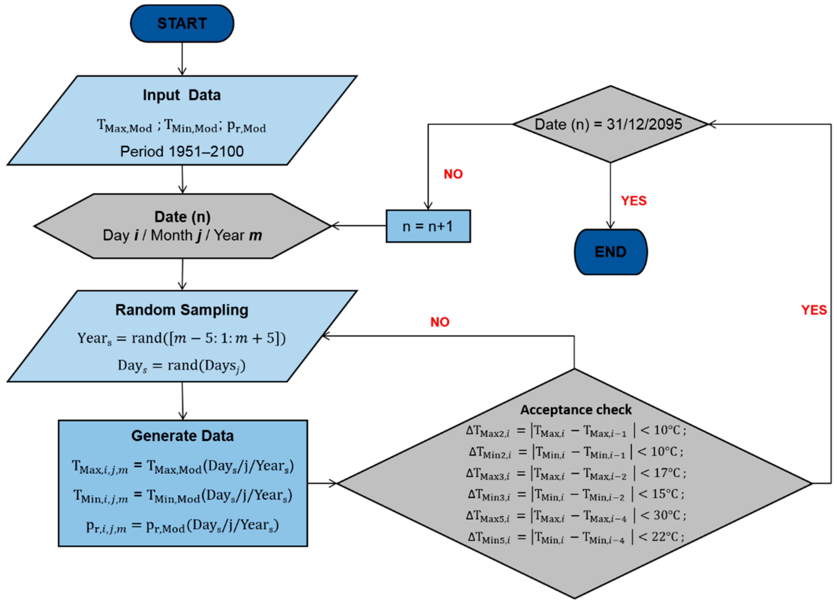
2.2. A Weather Generator for the Virtualization of the Outputs of Regional Climate Model

The innovative implementation of the weather generator algorithm proposed here aims to virtualize the outputs of Regional Climate Models. In “traditional” weather generation, random data are extracted from appropriate reference probability distribution functions (pdfs) or cumulative distribution functions (CDFs), whose relevant statistical parameters are derived fitting the statistics of climate variables derived from the climate model outputs. As anticipated, this kind of generation is sensitive to the assumptions, so that “errors” or “misinterpretations” of available information cannot be corrected in the subsequent phases. For this reason, the key feature of the proposed method is that data are generated directly sampling from the climate model outputs. The scheme of implementation of the algorithm and the fundamental steps of the procedure are summarized in the block diagram reported in Figure 1.
The basic information needed to start the generation algorithm is the output of the considered climate model. The typical climate model output is a series of climatic data, e.g., daily maximum and minimum shade air temperatures ( T Max , Mod and T Min , Mod ) and daily precipitation ( p r , Mod ), as those provided by high-resolution RCMs, selected among those included in EURO-CORDEX [47,48].
The procedure described in Figure 1 is applied for each considered model, to avoid inconsistencies in the generation, which could arise by mixing models characterized by different biases.
The generation of the daily information about the i -th day of the j -th month of the m -th year ( T Max , i , j , m , T Min , i , j , m and p r , i , j , m ) is performed randomly extracting the data from the output of the climate model concerning whichever day of the j -th months belonging to the considered year, and to the five consecutive years preceding or following the considered year, so that the time interval considered is 11 years long, from year m 5 to year m + 5 . This sampling period of 11 years has been chosen in such a way to properly modulate the contrasting needs of having a period, at the same time, long enough to assure adequately numerous data in the population, and short enough to exclude significant influence of climate change on climatic variables. Differently from [39,40], no specific probability is assigned to the set of days of the identified sampling period: in fact, a uniformly distributed sampling is performed.
To avoid the generation of unrealistic data, six additional constraints have been imposed for the acceptance of randomly generated daily data, as summarized in Equations (3)–(8); obviously, data not fulfilling the constraints are discarded and newly generated. Constraints refer to maximum and minimum temperatures variations in two consecutive days (Equations (3) and (4)), in three consecutive days (Equations (5) and (6)), and in five consecutive days (Equations (7) and (8)). The values, which are obviously depending on the country, or the geographical area considered in the study, need to be assessed analyzing actual data. For the relevant case study considered later in the paper, the following inequalities to be simultaneously fulfilled by the generated data in the i -th day have been established:
Δ T Max 2 , i , j , m =   T Max , i , j , m T Max , i 1 , j , m   < 10   ° C ,
Δ T Min 2 , i , j , m =   T Min , i , j , m T Min , i 1 , j , m   < 10   ° C ,
Δ T Max 3 , i , j , m =   T Max , i , j , m T Max , i 2 , j , m   < 17   ° C ,
Δ T Min 3 , i , j , m =   T Min , i , j , m T Min , i 2 , j , m   < 15   ° C ,
Δ T Max 5 , i , j , m =   T Max , i , j , m T Max , i 4 , j , m   < 30   ° C ,
Δ T Min 5 , i , j , m =   T Min , i , j , m T Min , i 4 , j , m   < 22   ° C .
The generation is carried out at each cell disregarding spatial correlation with the neighboring ones as the analysis of the extremes for the definition of climatic actions in structural design is not affected by their spatial behavior. Anyhow, in view of studies focusing on variables that are sensitive to spatial correlation, such as for example the total precipitation on large river basins, the procedure can be easily modified by implementing iterative steps to satisfy additional constraints between neighboring cells. With this aim, several suitable procedures can be envisaged, for example based on empirical limitations or on more refined analytical approaches. Empirical limitations could be defined considering recorded daily variations of climatic variables between adjacent cells. In this way, generated values are accepted only if the limitations are satisfied; if not, the sampling is iterated. A more refined approach could be based on the checking of the correlation length; in implementing the weather generation algorithm, the correlation length of the generated data series is checked against the correlation length of the original climate model output. Estimates of correlation functions and correlation lengths can be obtained from the experimental semi-variograms [49,50,51] of the original RCM output and of the generated series. When the estimated correlation length of the generated series is outside the confidence interval [51] of the original one, the generation is repeated.
By using the above-mentioned algorithm, a huge number of consistent series of daily maximum and minimum shade air temperatures ( T Max , i , j , m and T Min , i , j , m ) but also precipitations ( p r , i , j , m ) have been generated for the period 1956–2095, therefore not only covering the projected period but also the historical one. For the case study illustrated in the following, 1000 series are generated for each investigated climate model and scenario.
As far as the consistency of the generated precipitation series is concerned, specific checks at the cell level have been performed. The mean and coefficient of variation of daily precipitation, the fraction of wet days, and the mean wet-day amount calculated from the generated series are compared with those directly obtained analyzing the climate model output. As expected, the results show a very good agreement. As an example, in Table 1, the calculated parameters for the two series are compared for one cell in the study region (see Section 3.1) and for the period 1981–1990. Furthermore, it must be underlined that for the aims of the study, the focus is on the analysis of the extremes.
Performance metrics for the weather generation algorithms are evaluated by making use of the Taylor diagram [52], which relates the root mean square error (RMSE), the pattern correlation, and the standard deviation; the Taylor diagram is generally adopted to assess the ability of climate model simulations to reproduce observed climate statistics [53]. In this study, Taylor diagram and performance statistics are evaluated comparing the generated series and with the original climate model outputs. As an example, the results obtained for monthly mean statistics of daily maximum temperature are reported in Figure 2 with reference to the same cell, model and time period considered for the comparison in Table 1. As expected, a very good correlation is obtained between the simulations and the reference data as well as very low RMSE.
The analysis of the whole set of generated series, each one simulating one run of the climate model, allows evaluating the factors of change for convenient time intervals, as well as the confidence and the prediction intervals for the estimated changes over time.

2.3. Factors of Change and Extreme Values Theory

Analysis of climate extremes and evaluation of the values associated to a given probability of exceedance is generally performed resorting to the classical Extreme Value Theory, providing that the stationarity hypothesis is fulfilled. The basic concept of stationarity from which engineers work assumes that climate is variable but with variations whose properties are constant with time and that occur around an unchanging mean state [54]; i.e., given a time interval of fixed length, the statistical properties of the climatic variable are independent of the position of the time interval on the time axis. This assumption of stationarity is still common practice for the design criteria of new structures and infrastructures, and it is accepted for the time intervals generally considered in the elaboration of extremes of climatic variables, 40–50 years. However, considering the speed of current climate change, this assumption can become questionable; therefore, concepts and models able to take into account also variations of annual extremes over time are increasingly studied [55]. On the basis of these observations, an ad hoc procedure has been set up to evaluate the evolution of the extremes of climatic variables over time, in such a way to assess not only the influence of climate change on the extreme themselves, but also the consequences in terms of structural design.
The basic idea of this ad hoc procedure is that the influence of climate change on representative values of climatic variables can be captured studying the evolution of characteristic values over time. To perform this kind of assessment, it has been assumed that as long as the considered time period is shorter than 40 years, the stationarity hypothesis holds, and the internal influence of climate change can be disregarded; consequently, the tendency can be evaluated considering 40-year-long time periods (time windows) and assessing the variation over time of both the representative values of climatic variables and the statistical parameters of extreme value distributions. In the present study, the time shift between two consecutive time windows has been fixed to ten years.
As in structural design, characteristic values of climatic actions usually correspond to an annual probability of exceedance p = 2 % , this value has been assumed for the elaboration of extremes in each time window, also in view of using the outcomes of the study for the updating of climatic actions in specific sites, or, more generally, for updating of maps of climatic actions, such as those provided in Eurocodes; see e.g., [56] for a review of ground snow loads maps in Europe.
According to the methodology just sketched out, the artificially generated series of climatic data, extended from 1956 until 2095, have been subdivided into eleven time windows. For each time window, an annual extreme value analysis has been performed with the block maxima approach, assuming a Gumbel distribution and said extreme value type I distribution, whose CDF is:
F x < X , i = exp exp x μ i σ i       i = 1 , 11 ,       μ i   and   σ i > 0 ,  
where μ i and σ i are the parameters of the distribution, depending on the considered time window, i , to be estimated by means of a suitable method, for example, the least square method (LSM). The Gumbel distribution is assumed to be consistent with the prevailing model adopted in Europe for climatic actions in structural design [56,57], but the choice of the most appropriate distribution function is not straightforward and may depend on the investigated climate variable, the location, and the record length [29].
Thus, the characteristic values of the climatic variable, c k i , in the i -th time window are
c k i = μ i + σ i   ln ln 1 p   ,
where p is the annual probability of exceedance, for example p = 0.02 , as in Eurocodes.
An underestimation of extremes is generally detected from the analysis of climate model outputs [32,46,58,59,60]; therefore, to estimate future trends of climatic actions, a suitable calibration strategy should be adopted. Nevertheless, in the framework of the factor of change approach adopted in the present study, this kind of calibration is not needed, owing to the relative nature of the factor of change, which largely compensates the biases in climate projections if they will be maintained unchanged over time. In fact, the factor of change approach, which is widely used in climate impact research [58,61], represents a sound and easy calibration methodology.
The rationale of factors of change approach is the assumption that the actual changes over time of the observed climate variable y i are practically coincident with the ones predicted by the climate model. On this basis, x i p is the reference characteristic value of the considered climatic variable derived from the observations, y i p is its reference characteristic value obtained from the projections, x i f is the future characteristic value including the actual effects of climate change, and y i f is its future characteristic value obtained from the projections; thus, the following relationship can be established:
y i f y i p + x i f x i p ,
when factors of change are expressed in terms of differences, and
y i f y i p x i f x i p   ,
when factors of change are expressed in terms of quotient.
Actually, assuming that factors of change are nearly insensitive to absolute errors in the estimations of representative values, the proposed weather generation algorithm can provide sound estimates of factors of change of the investigated climate variable. The characteristic values obtained from the extreme value analysis of each generated series are compared considering the i -th time window, at the time 40 i 1 years, and the reference characteristic value obtained for the first time window ( i = 0 ). For extreme temperatures, the factor of change is defined in terms of differences
Δ T Max , k i = T Max , k 40 i 1 T Max , k 0
Δ T Min , k i = T Min , k 40 i 1 T Min , k 0
while a product factor of change in terms of quotient can be assessed for extreme precipitations
F C p r , k i = p r , k 40 i 1 p r , k 0 ,
and ground snow loads
F C s k i = s k 40 i 1 s k 0 .
The factors of change are evaluated for the whole set of generated series; thus, a significant ensemble is collected, allowing a probabilistic description of the expected changes for the extremes of the investigated climate variables.

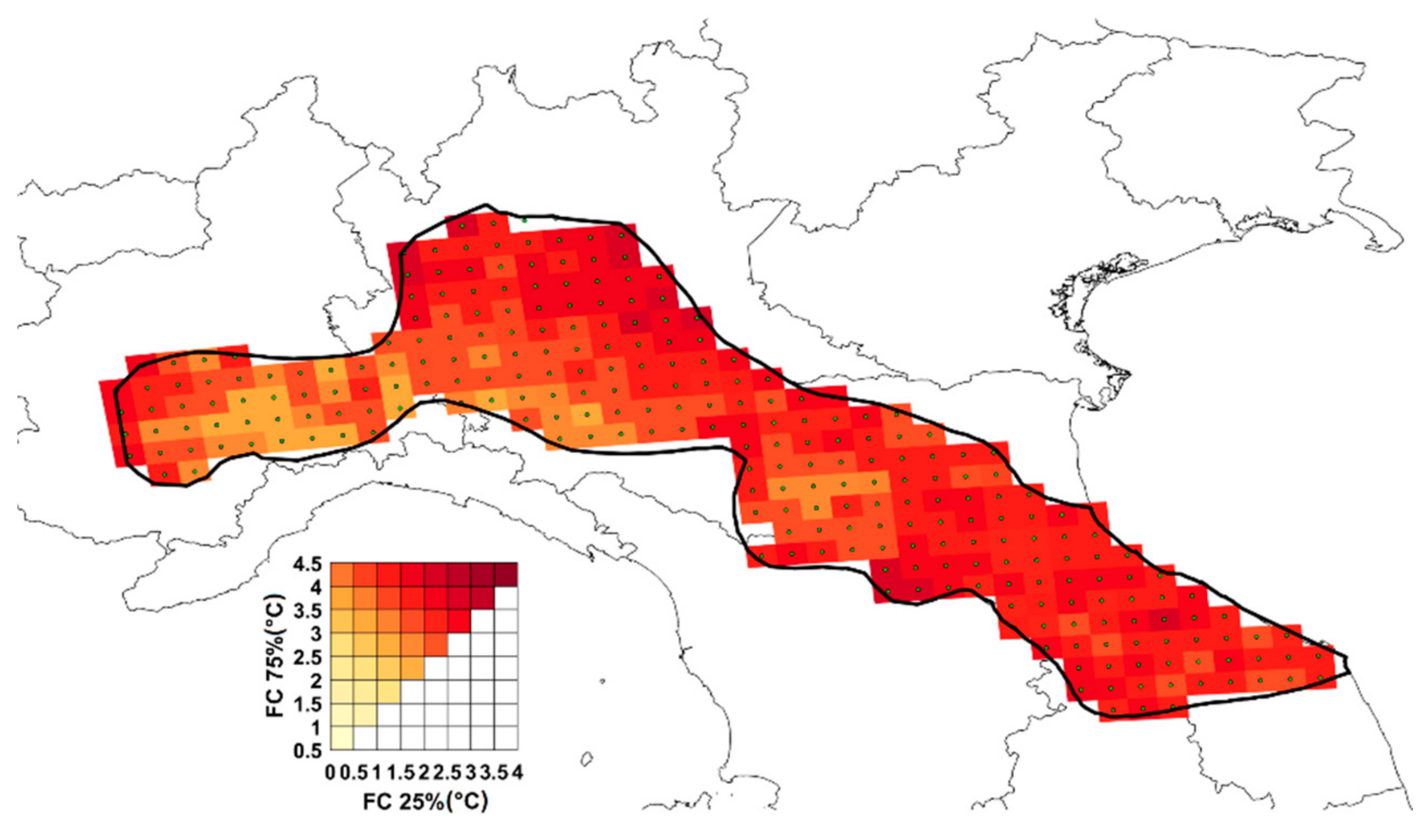
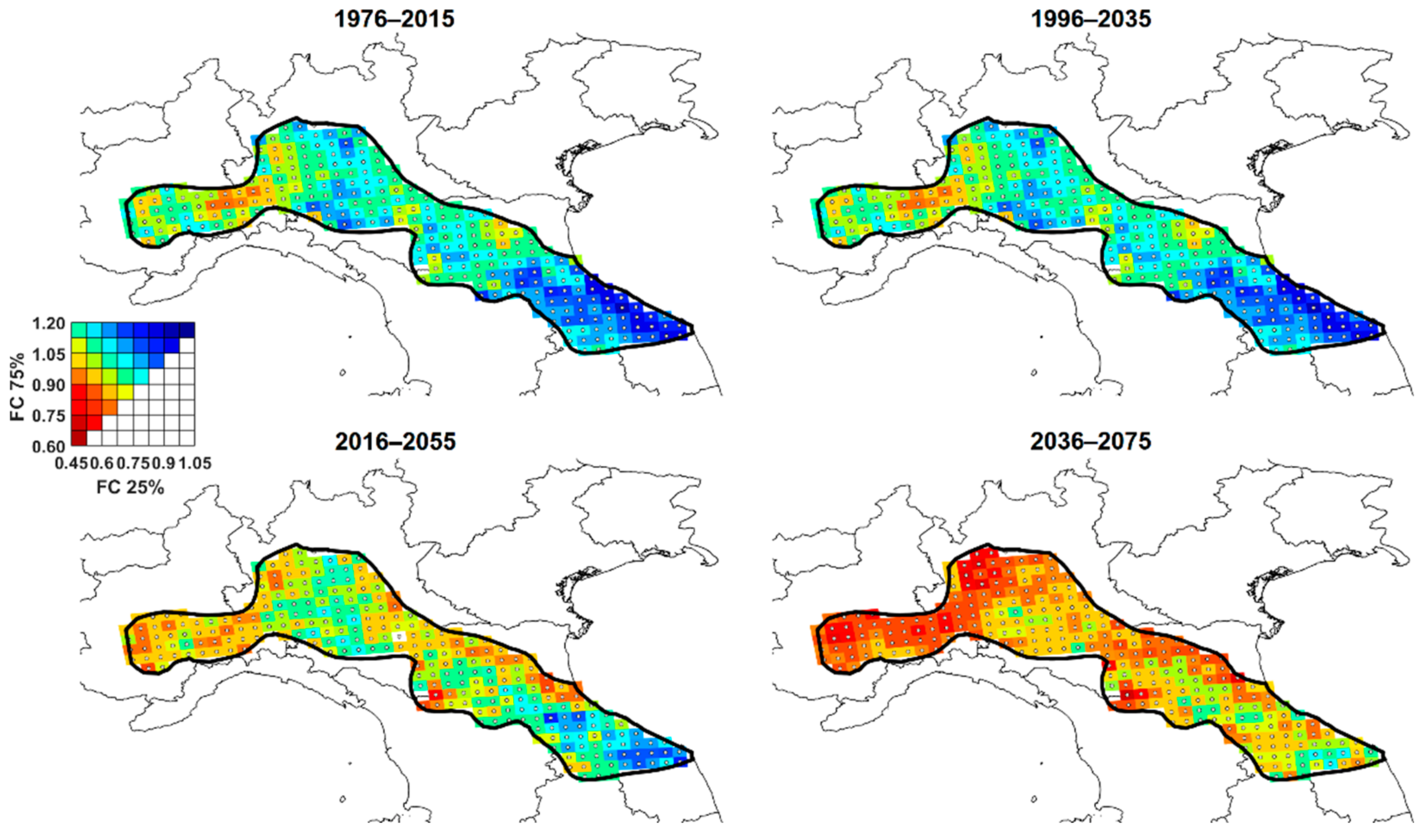
2.4. Factors of Change Maps

The analysis of the relevant outcomes obtained from the elaboration of generated series of climatic data allows deriving a significant collection of factors of change, satisfactorily describing the variation over time of the main statistical parameter characterizing the relevant climatic variables. In this way, prediction intervals corresponding to different percentiles of the factors of change ensemble can be determined, in such a way that changes in extreme values and pertinent uncertainty ranges can be highlighted. In the authors’ opinion, for the sake of practical applications, values corresponding to the 25th percentile and to the 75th percentile are particularly significant; therefore, in the following, they have been assumed as systematic reference, for the assessment of prediction intervals.
To show the potential and the effectiveness of the method, it has been applied to study the evolution over time of factors of changes in a relevant case study, regarding a central Eastern area of Italy, which belongs, as already said, to the so-called Mediterranean climatic zone, for which relevant factors of change maps have been derived, as illustrated in the following sections.
To make the reading of these maps easier, the results are represented as bivariate color maps [62], for each individual cell of a given area. This representation allows simultaneously drawing two limit percentiles in the same map, so giving an impressive illustration not only of the evolution over time of extremes values but also of the pertinent uncertainty interval. Moreover, these maps can be a useful platform to set up suitably modified climatic maps to be used in structural codes and standards, duly taking into account higher-level adaptation strategies. A significant example of such factors of change maps is illustrated in Figure 3, concerning the daily maximum temperatures in the cells of the Italian region considered in the case study. In the bivariate color map in Figure 3 and in the following ones as well, the color associated to each cell indicates, on the horizontal and vertical axis of the legend respectively, the lower and upper limits of the 25–75% prediction interval. For example, in Figure 3, the color corresponding to 1.75 °C on the horizontal axis and to 3.75 °C on the vertical axis is denoting a cell for which the 25–75% prediction limits are 1.75 °C and 3.75 °C.

3. Results

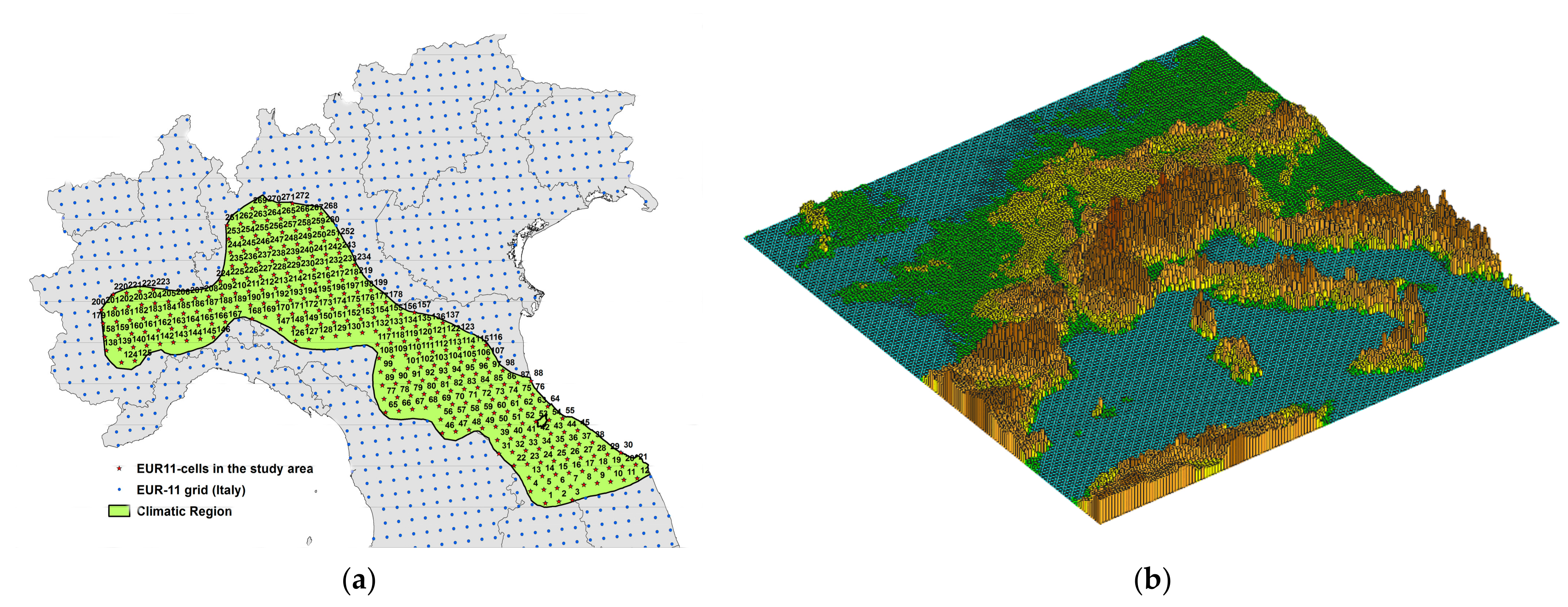
3.1. Study Area and Datasets

The procedure illustrated in the previous paragraph is applied here to investigate climate change impact on extreme temperatures and precipitation for the above-mentioned Italian region. Regarding snow loads, the studied area includes sites belonging to Zones 3 and 4 of the Mediterranean climatic region, as defined in EN1991-1-3:2003 [25]. These zones are illustrated in Figure 4a, together with the 272 cells for which high-resolution climate projections are available, being included in the EUR11 12.5 × 12.5 km grid of the Regional Climate Model of the EURO-CORDEX Figure 4b) [47,48].

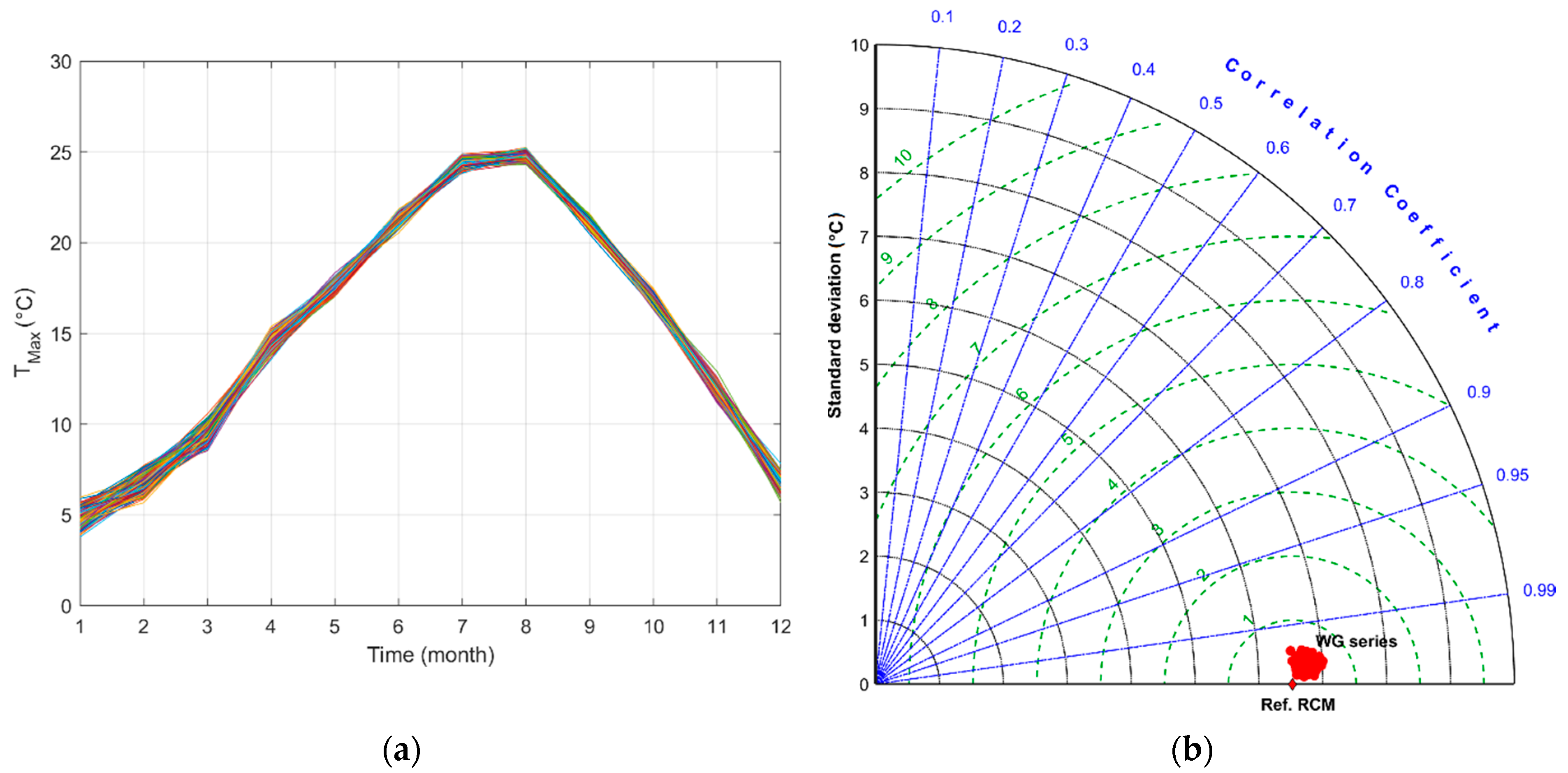
3.2. Dataset of Daily Maximum and Minimum Temperature

The dataset of climate projections considered in the study covers the period 1951–2100. The above-mentioned period is split in two parts: a control period, from 1951 until 2005, and a future period, 2006–2100. The control period is used for the so-called Historical Experiment, aiming to assess the capability of the climate model to reproduce past weather: in this run, the observed changes in the greenhouse gas content of the atmosphere are forced in the model, checking the agreement between the predictions of the model and actual observations. The future period is used for projections in the RCPs Experiment, where the runs of the model are forced according to various scenarios, which are characterized by the assumed atmospheric composition changes described by various representative concentration pathways (RCPs) [54]. The scenarios mostly considered in climate risk studies are RCP4.5 and RCP8.5, for which the majority of climate projections are available. They correspond to medium and maximum greenhouse gas emission pathways, and they have been adopted in the present study as well, even if the discussion on climate scenarios is rapidly evolving and at present, RCP4.5 appears to offer more realistic baselines [63], while the use of RCP8.5 is debated by the scientific community [42,64], often appearing excessively pessimistic. Moreover, the discussion is even more complex, since it is influenced not only by the input greenhouse gasses emissions but also by the output of the models.
Regarding the historical experiment, climatic data provided by several meteorological institutes, namely the Laboratoire des Sciences du Climat et de l’Environnement, Institut Pierre Simon Laplace, IPSL-INERIS, the Max Planck Institute, MPI-CSC, the Royal Netherlands Meteorological Institute (KNMI), and the Danish Meteorological Institute, were processed. The same research institutes also provided the climate projections considered in the assessment of variations of climatic variables induced by climate change. A synthetic description and the main characteristics of each model are summarized in Table 2.
The results presented in the following sections are derived applying the proposed weather generation algorithm starting from the multi-model ensemble, which is obtained combining the individual climate models and adopting a constant weight for each of them, so hypothesizing that each model is equally suitable to reproduce the effects of climate change over time. The rationale of considering a model ensemble is that each model of the ensemble can be generally considered as the result of a reasonable, independent sampling of future climate. Truly, a further refinement could be introduced, suitably weighing the climate models, i.e., modifying the individual weight of each model, based on their ability to reproduce past observations [65], but this topic involves very complicated and delicate aspects, which cannot be easily tackled in a general way.

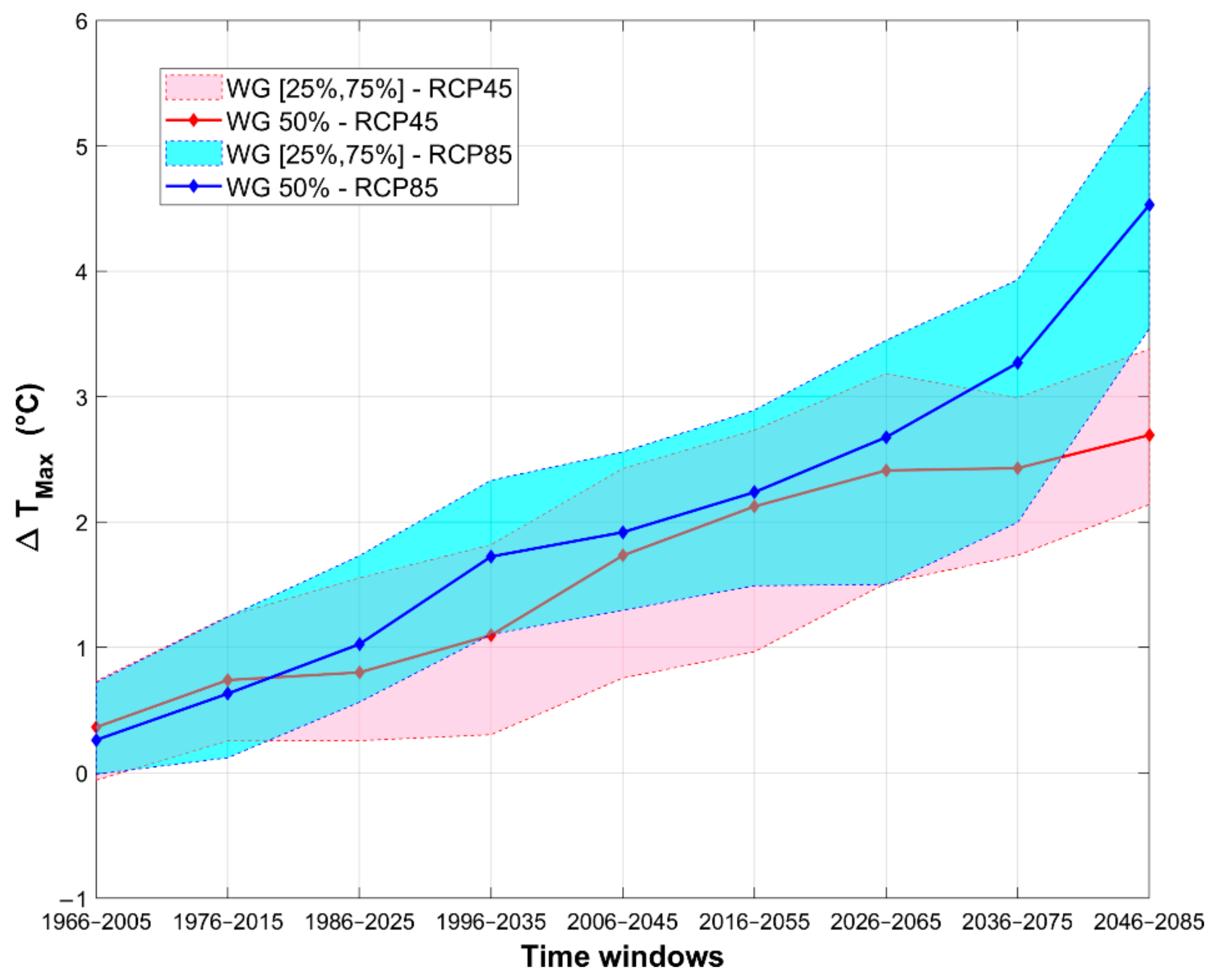
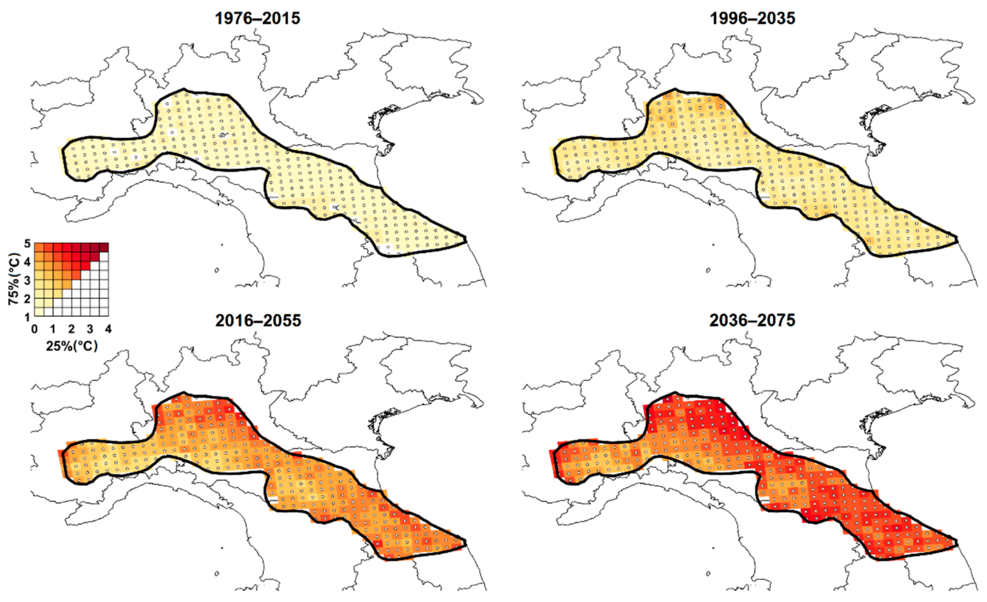
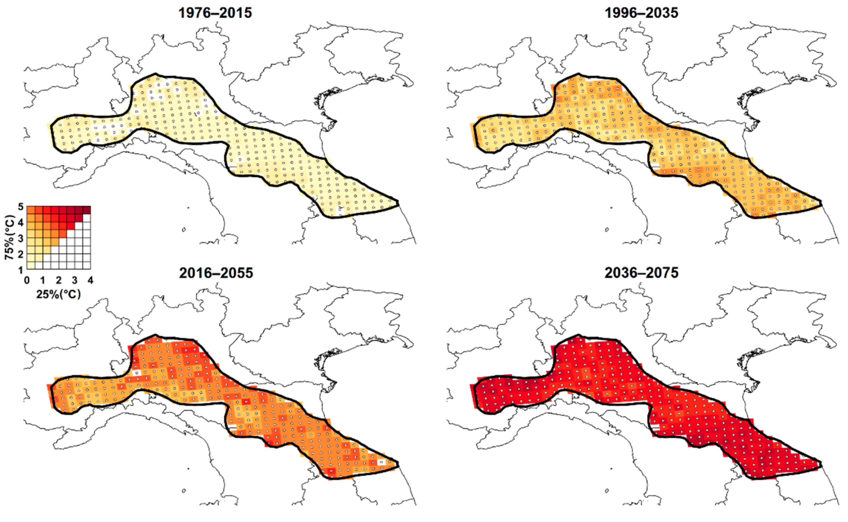
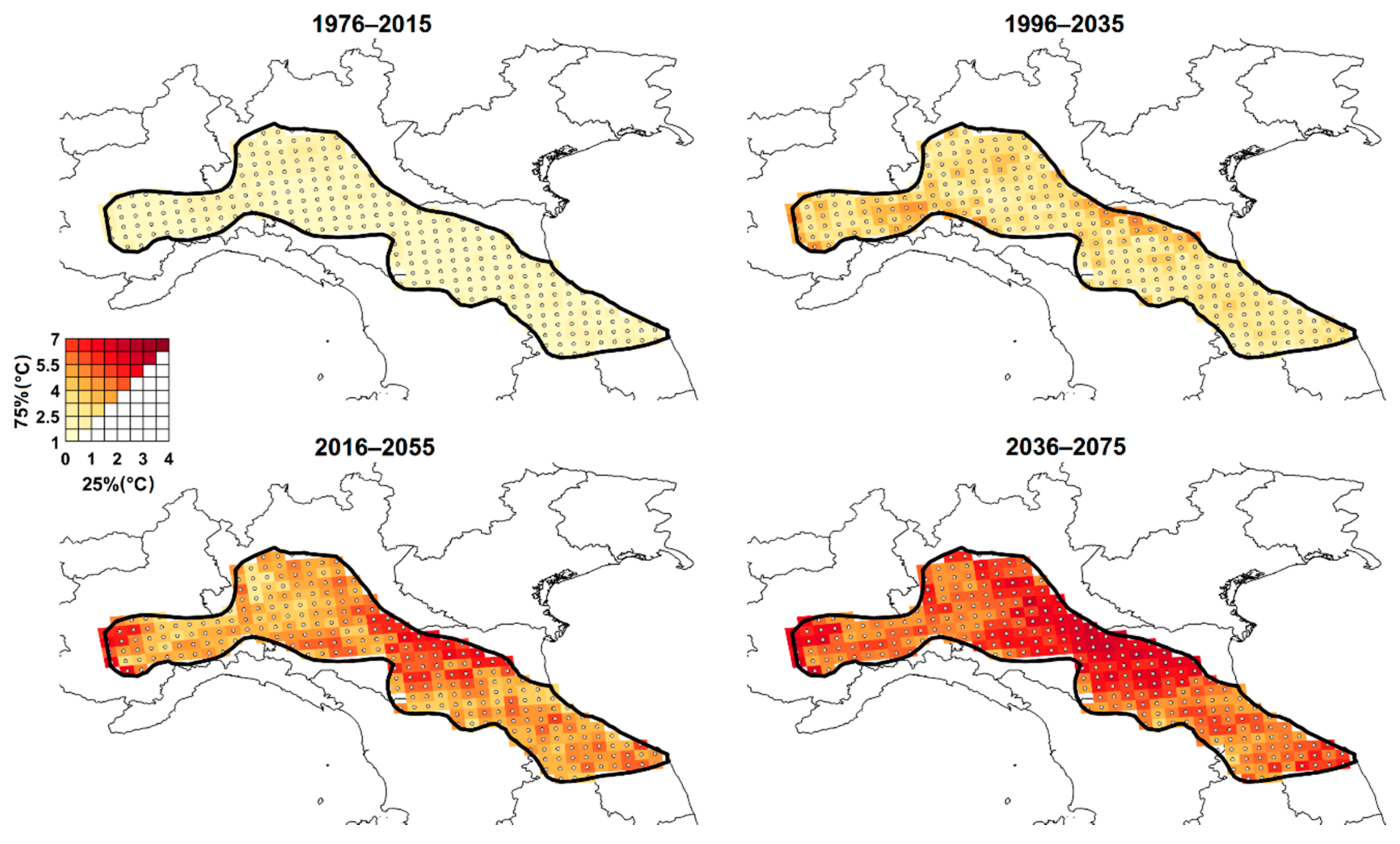
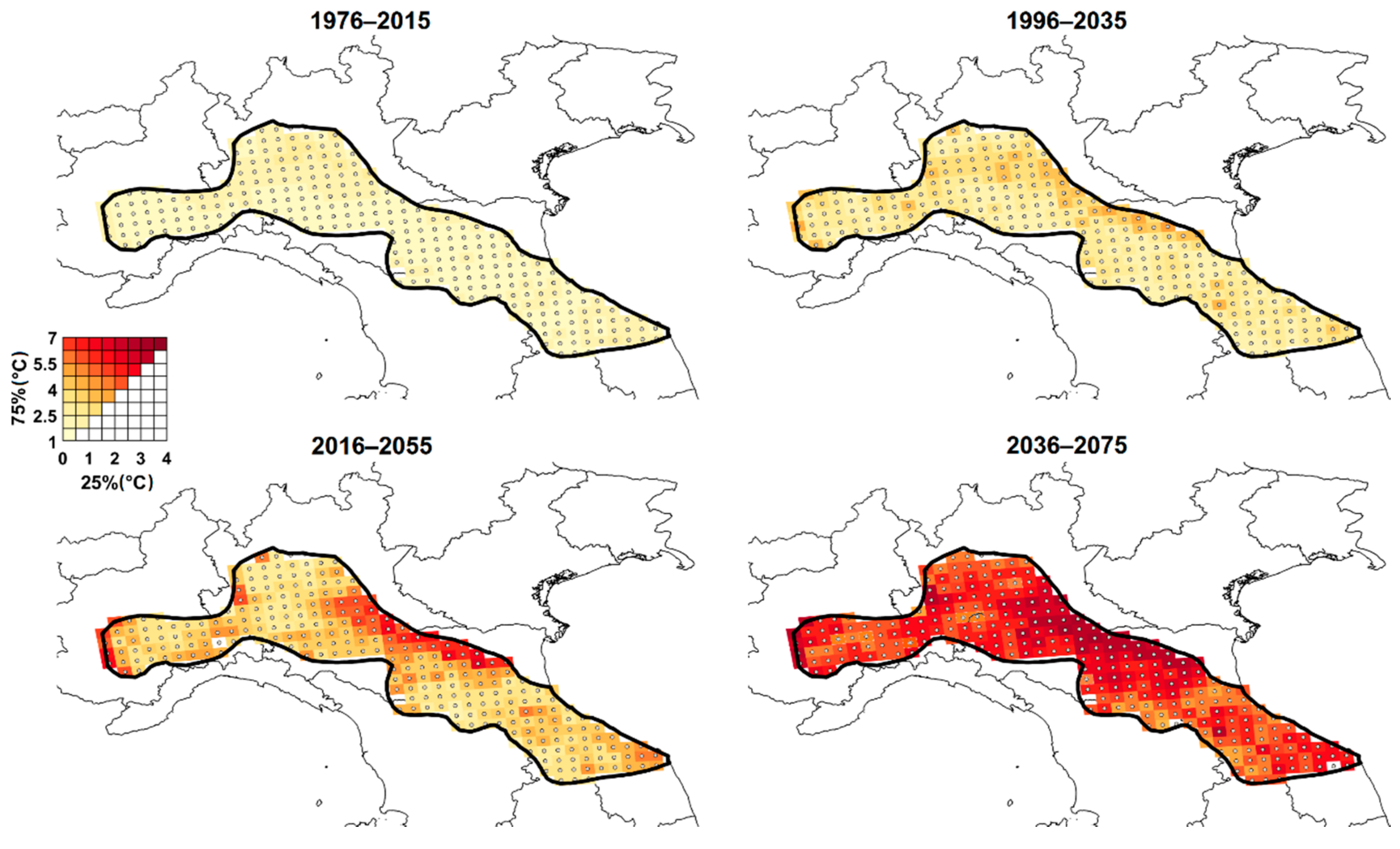
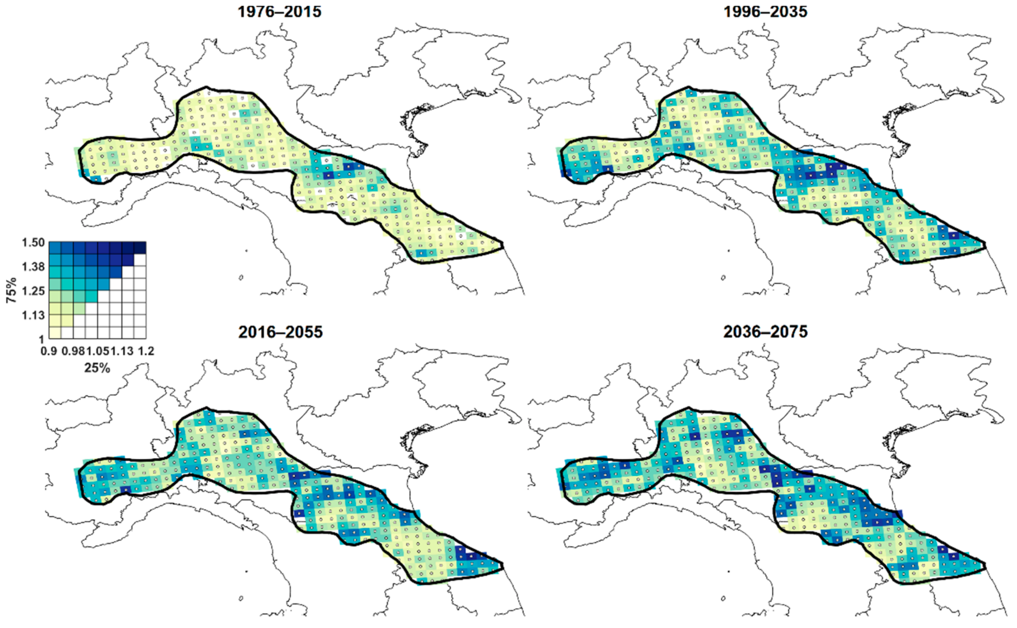
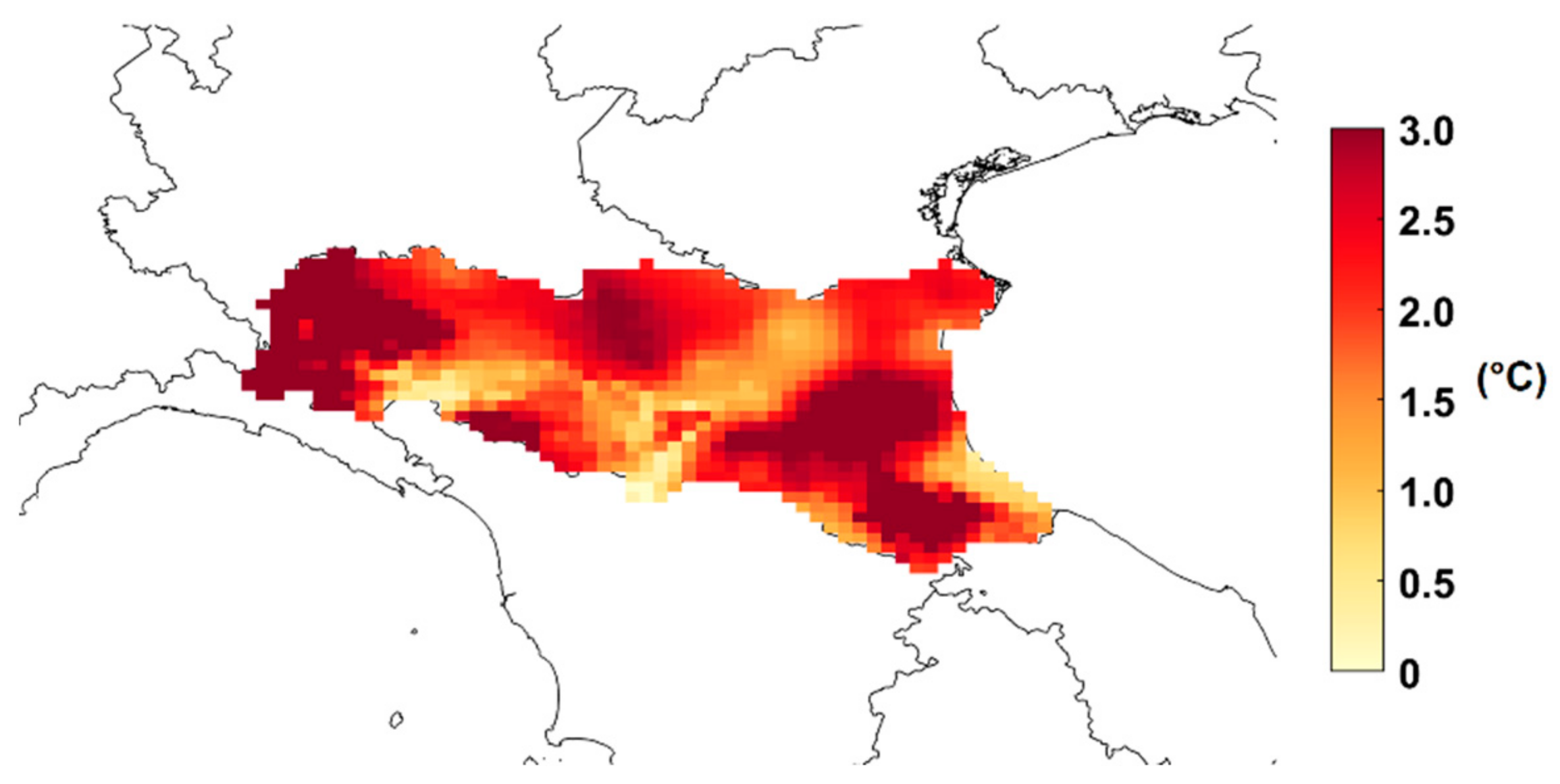
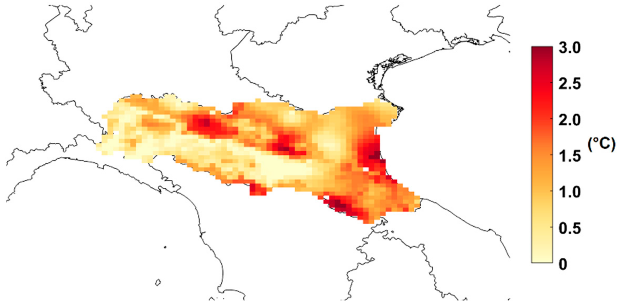
3.3. Effects of Climate Change on Extreme Temperatures

By means of the new weather generator algorithm previously described, factors of change and suitable prediction intervals have been assessed, in comparison with the reference time window, 1956–1995 for characteristic values of daily maximum and minimum temperature, T Max , k and T Min , k , in each individual cell of the studied region. Of course, as the considered climatic variable is the temperature, factors of change have been derived in terms of differences [66], according to Equations (13) and (14).
A first example of the obtained results is shown in Figure 5, where factors of change in terms of differences are reported for characteristic values of maximum temperature in one cell of the investigated region (cell 101). Trends are illustrated for the two considered scenarios together with the associated uncertainty, i.e., the prediction interval 25–75%.
The main outcomes of the study are summarized in the factors of change maps, as illustrated in Figure 6 and Figure 7, for the RCP4.5 and RCP8.5 scenarios, respectively. In the bivariate maps, the characteristic values of daily maximum air shade temperature ( T Max , k ) in four significant time windows (1976–2015, 1996–2032, 2016–2055, and 2035–2075) are illustrated, referring to the 25th and the 75th percentile.
Table 3 summarizes the average factors of change obtained in the investigated region according to the RCP4.5 and RCP8.5 emission scenarios. In the table, results corresponding to prediction percentiles 25%, 50%, and 75% are given for each time window considered in the study.
Characteristic values of daily minimum air shade temperature ( T Min , k ) are illustrated in a similar way in Figure 8 and Figure 9, while analogously to what was previously done for maximum temperature, the factors of change percentiles (25%, 50%, 75%) averaged over the region are summarized in Table 4 for each time window.
The results confirm that there is a high probability that extreme temperatures significantly rise over time. This tendency accords with the expectations about mean temperatures [67], but it emerges more markedly, confirming the conclusions obtained analyzing actual measurements [29].
For example, considering the time window 2036–2075, the lower and upper limits of the prediction interval of the increase of the characteristic value of the maximum temperature are 1.87 °C and 3.55 °C, respectively, with an average value of 2.75 °C, considering the RCP4.5 scenario, and 2.47 °C and 4.17 °C, respectively, with an average value of 3.37 °C, considering the RCP8.5 scenario. In the same time window 2036–2075, a more pronounced rise is expected for T Min , k : the lower and upper limits of the prediction interval of the increase of the characteristic value of the minimum temperature are 2.47 and 4.17 °C, respectively, with an average value of 3.37 °C, considering the RCP4.5 scenario, and 2.29 and 5.23 °C, respectively, with an average value of 3.52 °C, considering the RCP8.5 scenario.
Clearly, on the basis of these observations, suitable updates of current temperature maps provided in the Italian National Annex to EN1991-1-5:2003 [27] seem to be necessary.

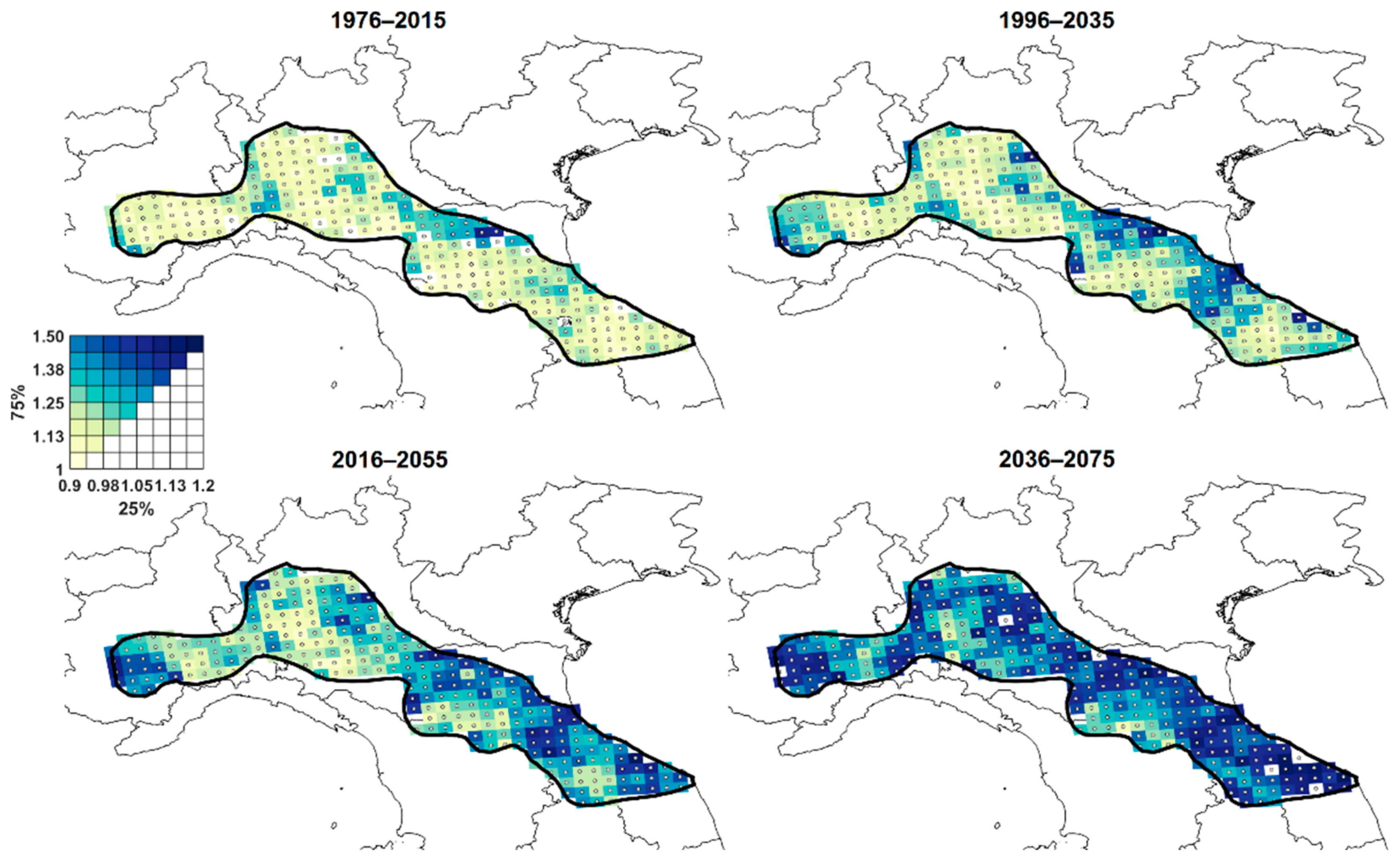
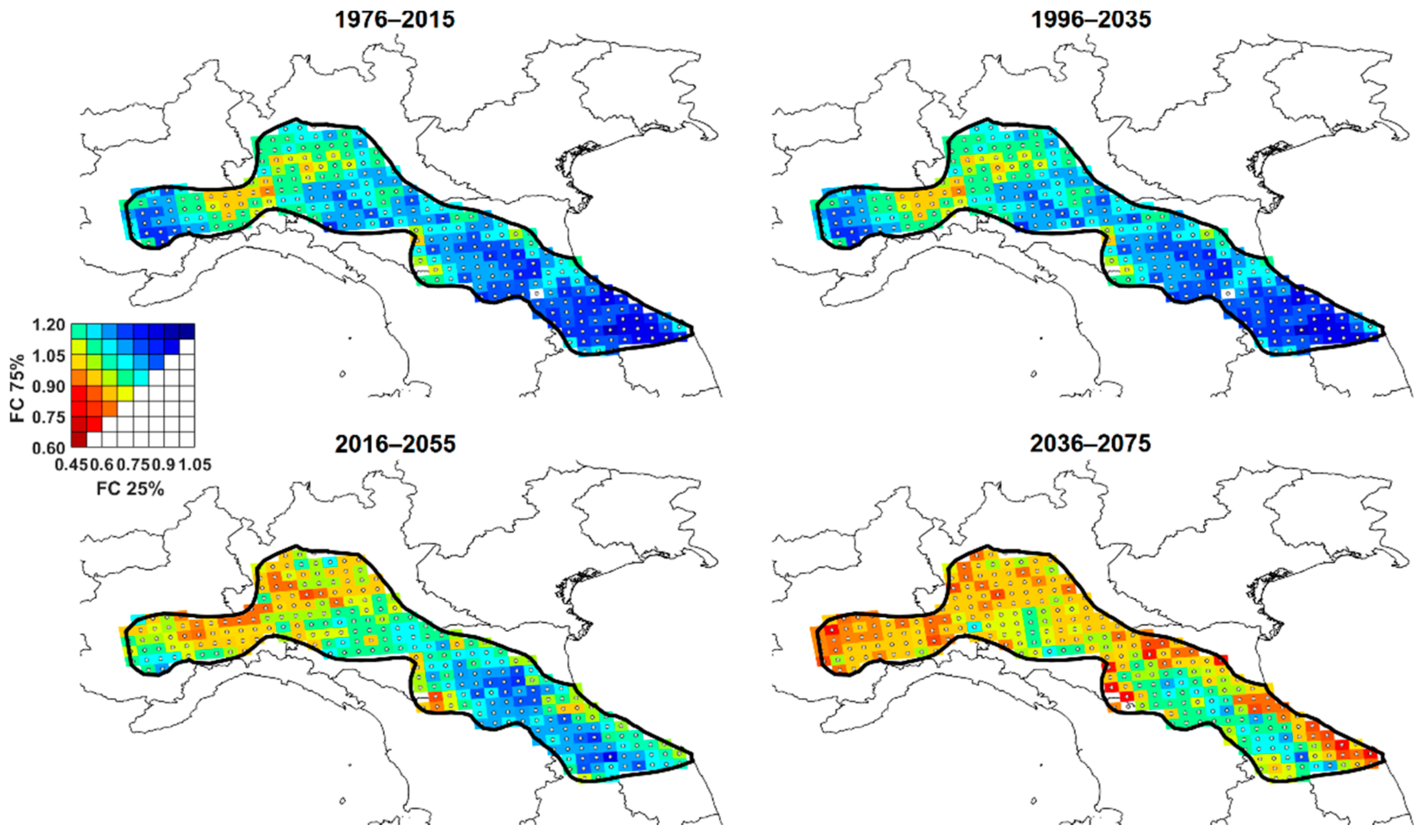
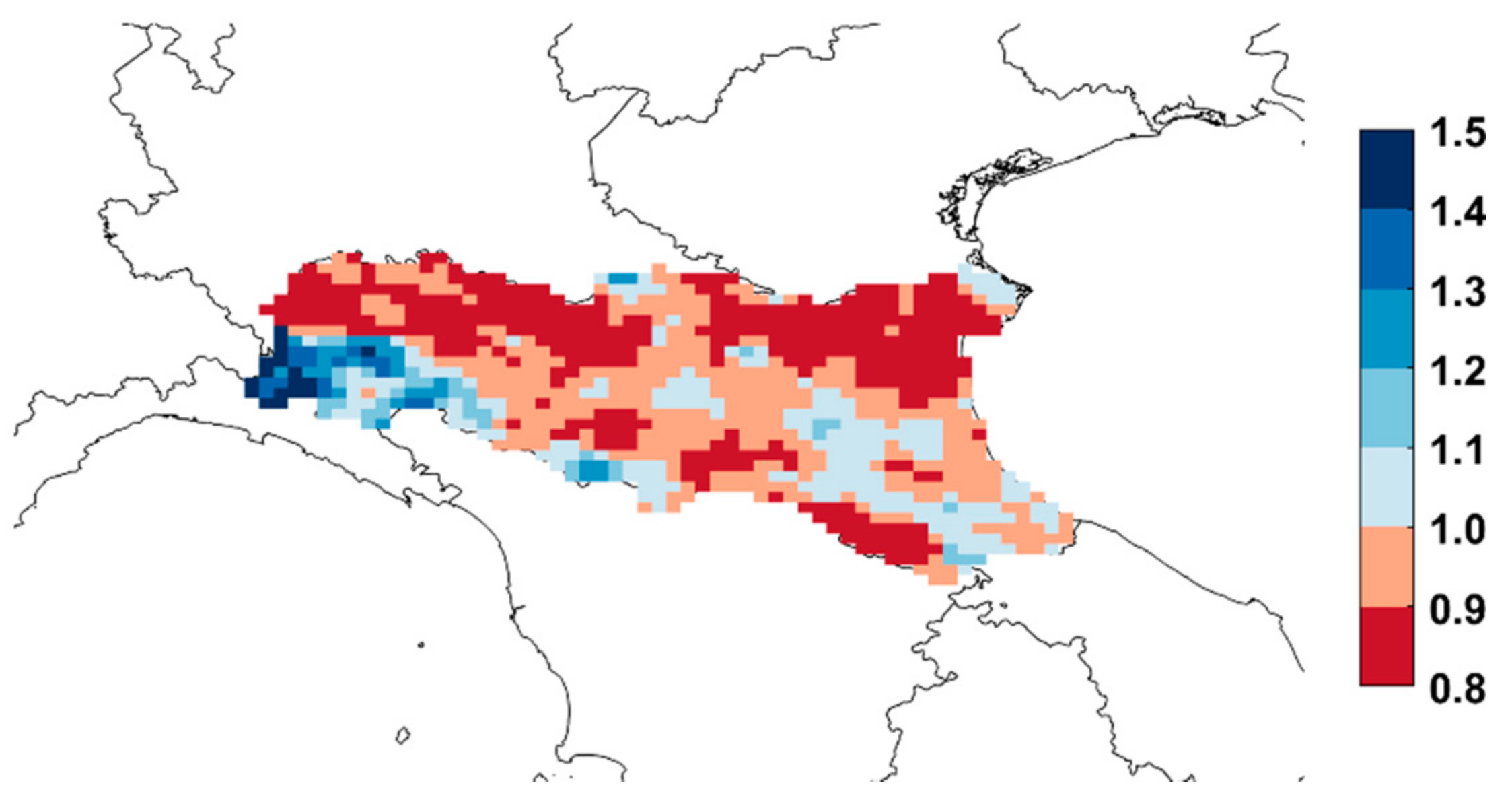
3.4. Effects of Climate Change on Extreme Precipitation

Regarding the effects of climate change on rainfalls, there is observational evidence that the frequency and intensity of heavy rainfalls is increasing in several regions all around the world. This evidence is further validated by the outcomes of many recent research works [68,69]. This observation is in close agreement with the classical thermodynamic law, also known as Clausius–Clapeyron law, stating that warmer the air, the higher its capacity to hold water vapor [70,71]. Looking only at the increase of atmospheric moisture content, a scaling rate of warming around 6–7% K 1 can be predicted, according to the recalled Clausius–Clapeyron law.
Considering an annual probability of exceedance p = 2 % , factors of change of characteristic values of daily precipitation ( p r , k ) and associated prediction intervals have been also derived by means of the proposed weather generator.
Factors of change maps for characteristic values of precipitation ( p r , k ) and associated prediction intervals for time windows 1976–2015, 1996–2035, 2016–2055, and 2035–2075 are presented in the bivariate maps reported in Figure 10 and Figure 11, referring to the RCP4.5 and RCP8.5 scenarios, respectively. Evidently, in this case, as in the next one concerning snow loads, factors of changes are derived in form of quotients, according to Equation (15).
Factors of change percentiles (25%, 50%, 75%), averaged over the region, are summarized in Table 5 for each time window.

3.5. Ground Snow Loads

Starting from the generated samples of daily temperatures and precipitation (Tmax, Tmin and pr), they have been assessed the characteristic values of the snow load on ground. Since the estimation of ground snow load requires reconstructing the complicated processes governing snowfall, snow accumulation, total or partial melting of the snow cover, and so on, the application of a weather generation algorithm has been supplemented with the procedure developed by the authors to simulate snow load on the ground on the basis of precipitation and temperature data [6,7], so obtaining characteristic values of snow load in each 40-year-long time window.
For the investigated region, factors of change maps, concerning characteristic ground snow load, s k , in time windows 1976–2015, 1996–2035, 2016–2055, and 2036–2075, in comparison with the reference time window 1956–1995, are presented in Figure 12 and Figure 13, for the RCP4.5 and RCP8.5 scenarios, respectively.
The outcomes confirm that the investigated region is characterized by a general decreasing trend, even if locally different behavior can be detected, depending on the grid cell, on the investigated time window, and on the considered scenario. In fact, as already highlighted by O’Gorman in [72], the reduction of snowfall fraction and the increase of heavy precipitation caused by global warming, may locally lead to a contrasting response in terms of snowfall variation. On the one hand, the temperature rise facilitates the melting of snow and increases the fraction of precipitation falling as rain; on the other hand, it is associated with a rise of precipitation rate during extreme events, potentially leading to heavy snowfalls and higher ground snow load. Thus, the overall outcome, in terms of increase or decrease of the ground snow load, is dependent on the ratio of these two competing factors [73].
Nevertheless, according the obtained results, in the near future (1996–2035), a constant or increasing trend (FC50% > 0.95) can be expected in around 15% of the region in the RCP4.5 scenario, and in around 7% of the region in the RCP8.5 scenario. However, a decrease is expected in the long-term future (2036–2075) for the whole region.
As previously done for precipitation, the results are averaged over all grid cells to better visualize changes in ground snow load, reducing the influence of unforced variability at the grid box level. The resulting factors of change in the considered time windows, averaged on the region, are reported for the given prediction percentiles (25%, 50%, and 75%) in Table 6. The results confirm that the ground snow loads in the investigated region generally decrease, by approximately 10% to 15% in the time interval 1991–2030 and 25% to 30% in the future (2041–2080). Moreover, the obtained results are practically independent on the considered RCP scenario.

4. Discussion

As already mentioned in the introduction, the aim of the present study is to provide a methodology for the treatment of climate model outputs by means of a weather generation technique combined with the factor of change approach. The results obtained for the case study presented in Section 3 show the suitability of the methodology but are not intended to represent a detailed guidance for adaptation planning.
Dealing with regional climate projections, the skill of the ensemble to reproduce multidecadal changes in the study region should be first assessed. This can be carried out by comparing the variation of climate statistics provided by the climate model ensemble and by the available high-resolution observational dataset for the historical period. As an example, factors of change for daily temperatures and precipitation can be evaluated for a part of the investigated region from the analysis of the Eraclito-ERG5 dataset [74]. The Eraclito-ERG5 is a high-quality gridded observational dataset for the Emilia Romagna region in Italy, covering the period 1961–2020 and characterized by a horizontal resolution of about 5 km × 5 km.
In Figure 14, Figure 15 and Figure 16, factors of change for characteristic values of daily maximum and minimum temperature, and daily precipitation are reported for the time window 1981–2020 with respect to the period 1961–2000. Trends are generally consistent with those previously presented in Section 3; local differences can be justified remarking on the one hand that the database of observations and climate projections have different resolutions, on the other that the time windows are not perfectly coincident. Of course, the output of climate models with this extremely refined resolution could significantly improve the evaluation of climate change impacts. The wish is that they will soon be available.

5. Conclusions

In the paper, a new procedure for the analysis of climate model outputs is presented in view of a probabilistic assessment of future trends of climatic actions.
The proposed methodology is based on an innovative weather generator, which investigates the internal variability of climate models and allows improving the statistical representativeness of the climate model ensemble, preserving the consistency of the original climate model output. In fact, performance metrics have shown a very good agreement between the statistics of the generated series and the original ones for daily temperatures and precipitation.
Thus, the generated series can be used to investigate changes in the statistics of climatic variables, e.g., temperatures and precipitation, providing a quantification of the uncertainty associated with the predicted changes.
The results, presented for different climatic actions, in terms of confidence maps for the study region in Italy, confirm that the technique is very promising and can be successfully applied for the adaptation of climatic actions maps given in codes and standards for structural design. For example, starting from the obtained FC maps, current thermal and ground snow load maps based on past observations and provided in the Italian National Annex to Eurocode EN1991-1-5 [27] and EN1991-1-3 [25] respectively can be updated considering climate change impacts [75]. As the soundness of the output of the method is a function of the quality and of the resolution of climate models, it will be improved as soon as the next generation of climate projections will be available.

Author Contributions

Conceptualization, P.C., P.F. and F.L.; methodology, P.C., P.F. and F.L.; software, P.C., P.F. and F.L.; validation, P.C., P.F. and F.L.; data curation, P.C., P.F. and F.L.; writing—original draft preparation, P.C., P.F. and F.L.; writing—review and editing, P.C., P.F. and F.L.; visualization, P.C., P.F. and F.L.; resources, P.F. All authors have read and agreed to the published version of the manuscript.

Funding

This research received no external funding.

Institutional Review Board Statement

Not applicable.

Informed Consent Statement

Not applicable.

Data Availability Statement

The data presented in this study are available on request from the corresponding author. The data are not publicly available as they cannot be used for commercial purposes.

Acknowledgments

The authors acknowledge the World Climate Research Working Groups on Regional Climate, and on Coupled Modelling. The authors thank the climate modeling groups listed in Table 2 for providing the model outcomes via the infrastructure of the Earth System Grid Federation (https://esgf-data.dkrz.de/search/cordex-dkrz/, accessed on 18 August 2021).

Conflicts of Interest

The authors declare no conflict of interest.

References

  1. Bastidas-Arteaga, E.; Stewart, M. Climate Adaptation Engineering; Butterworth-Heinemann: Oxford, UK, 2019. [Google Scholar]
  2. Madsen, H.O. Managing structural safety and reliability in adaptation to climate change. In Safety, Reliability, Risk and Life-Cycle Performance of Structures and Infrastructure; CRC Press: Boca Raton, FL, USA, 2013; pp. 81–88. [Google Scholar]
  3. Stewart, M.G.; Deng, X. Climate impact risks and climate adaptation engineering for built infrastructure. ASCE-ASME J. Risk Uncertain. Eng. Syst. Part A Civ. Eng. 2015, 1, 04014001. [Google Scholar] [CrossRef]
  4. Croce, P.; Formichi, P.; Landi, F. Climate change: Impacts on climatic actions and structural reliability. Appl. Sci. 2019, 9, 5416. [Google Scholar] [CrossRef] [Green Version]
  5. Forzieri, G.; Bianchi, A.; Batista e Silva, F.B.; Herrera, M.A.M.; Leblois, A.; Lavalle, C.; Aerts, J.C.J.H.; Feyen, L. Escalating impacts of climate extremes on critical infrastructures in Europe. Glob. Environ. Chang. 2018, 48, 97–107. [Google Scholar] [CrossRef] [PubMed]
  6. Croce, P.; Formichi, P.; Landi, F. Structural safety and design under climate change. In 20th Congress of IABSE, New York City 2019: The Evolving Metropolis; International Association for Bridge and Structural Engineering (IABSE): Zurich, Switzerland, 2019; pp. 1130–1135. [Google Scholar]
  7. Croce, P.; Formichi, P.; Landi, F.; Marsili, F. Climate change: Impact on snow loads on structures. Cold Reg. Sci. Technol. 2018, 150, 35–50. [Google Scholar] [CrossRef] [Green Version]
  8. Croce, P.; Formichi, P.; Landi, F.; Mercogliano, P.; Bucchignani, E.; Dosio, A.; Dimova, S. The snow load in Europe and the climate change. Clim. Risk Manag. 2018, 20, 138–154. [Google Scholar] [CrossRef]
  9. Forzieri, G.; Bianchi, A.; Herrera, M.A.M.; Batista e Silva, F.; Lavalle, C.; Feyen, L. Resilience of Large Investments and Critical Infrastructures in Europe to Climate Change; EUR27906; Publications Office of the European Union: Luxembourg, 2016. [Google Scholar] [CrossRef]
  10. Organization for Economic Co-Operation and Development (OECD). Climate-Resilient Infrastructure; OECD ENVIRONMENT POLICY PAPER NO. 14; OECD Publishing: Paris, France, 2018. [Google Scholar]
  11. Intergovernmental Panel on Climate Change (IPCC). Climate Change 2021: The Physical Science Basis. Contribution of Working Group I to the Fifth Assessment Report of the Intergovernmental Panel on Climate Change—Summary for Policymakers; Cambridge University Press: Cambridge, UK, 2021. [Google Scholar]
  12. Pryor, S.C.; Barthelmie, R.J.; Bukovsky, M.S.; Leung, L.R.; Sakaguchi, K. Climate change impacts on wind power generation. Nat. Rev. Earth Environ. 2020, 1, 627–643. [Google Scholar] [CrossRef]
  13. Wagner, T.; Themeßl, M.; Schüppel, A.; Gobiet, A.; Stigler, H.; Birk, S. Impacts of climate change on stream flow and hydro power generation in the Alpine region. Environ. Earth Sci. 2017, 76, 4. [Google Scholar] [CrossRef] [Green Version]
  14. Christodoulou, A.; Christidis, P.; Bisselink, B. Forecasting the impacts of climate change on inland waterways. Transp. Res. Part D Transp. Environ. 2020, 82, 102159. [Google Scholar] [CrossRef]
  15. Konapala, G.; Mishra, A.K.; Wada, Y.; Mann, M.E. Climate change will affect global water availability through compounding changes in seasonal precipitation and evaporation. Nat. Commun. 2020, 11, 3044. [Google Scholar] [CrossRef]
  16. Mbow, C.C.; Rosenzweig, L.G.; Barioni, T.G.; Benton, M.; Herrero, M.; Krishnapillai, E.; Liwenga, P.; Pradhan, M.G.; Rivera-Ferre, T.; Sapkota, F.N.; et al. Food security. In Climate Change and Land: An IPCC Special Report on Climate Change, Desertification, Land Degradation, Sustainable Land Management, Food Security, and Greenhouse Gas Fluxes in Terrestrial Ecosystems; Cambridge University Press: Cambridge, UK, 2019. [Google Scholar]
  17. Stewart, M.G.; Wang, X.; Nguyen, M. Climate change impact and risks of concrete infrastructure deterioration. Eng. Struct. 2011, 33, 1326–1337. [Google Scholar] [CrossRef]
  18. Bastidas-Arteaga, E.; Schoefs, F.; Stewart, M.G.; Wang, X. Influence of global warming on durability of corroding RC structures: A probabilistic approach. Eng. Struct. 2013, 51, 259–266. [Google Scholar] [CrossRef] [Green Version]
  19. Bisoi, S.; Haldar, S. Impact of climate change on design of offshore wind turbine considering dynamic soil–structure interaction. J. Offshore Mech. Arct. Eng. 2017, 139, 061903. [Google Scholar] [CrossRef]
  20. Hoekstra, A.Y.; De Kok, J.L. Adapting to climate change: A comparison of two strategies for dike heightening design. Nat. Hazards 2008, 47, 217–228. [Google Scholar] [CrossRef] [Green Version]
  21. Lutz, J.; Dobler, A.; Nygaard, B.E.; Mc Innes, H.; Haugen, J.E. Future projections of icing on power lines over Norway. In Proceedings of the International Workshop on Atmospheric Icing of Structures IWAIS 2019, Reykjavík, Iceland, 23–28 June 2019. [Google Scholar]
  22. Faggian, P.; Bonanno, R.; Pirovano, G. Research activities to cope with wet snow impacts on overhead power lines in future climate over Italy. In Proceedings of the International Workshop on Atmospheric Icing of Structures IWAIS 2019, Reykjavík, Iceland, 23–28 June 2019. [Google Scholar]
  23. Hirabayashi, Y.; Mahendran, R.; Koirala, S.; Konoshima, L.; Yamazaki, D.; Watanabe, S.; Kim, H.; Kanae, S. Global flood risk under climate change. Nat. Clim. Chang. 2013, 3, 816–821. [Google Scholar] [CrossRef]
  24. European Committee for Standardization (CEN). EN 1990. Eurocode—Basis of Structural Design; CEN: Brussels, Belgium, 2002. [Google Scholar]
  25. European Committee for Standardization (CEN). EN 1991-1-3. Eurocode 1: Actions on Structures—Part 1–3: General Actions—Snow Loads; CEN: Brussels, Belgium, 2003. [Google Scholar]
  26. European Committee for Standardization (CEN). EN 1991-1-4. Eurocode 1: Actions on Structures—Part 1–4: General Actions—Wind Actions; CEN: Brussels, Belgium, 2005. [Google Scholar]
  27. European Committee for Standardization (CEN). EN 1991-1-5. Eurocode 1: Actions on Structures—Part 1–5: General Actions—Thermal Actions; CEN: Brussels, Belgium, 2003. [Google Scholar]
  28. International Organization for Standardization (ISO). ISO 2394 General Principles on Reliability for Structures; ISO: Geneva, Switzerland, 2015. [Google Scholar]
  29. Croce, P.; Formichi, P.; Landi, F. Evaluation of current trends of climatic actions in Europe based on observations and regional reanalysis. Remote Sens. 2021, 13, 2025. [Google Scholar] [CrossRef]
  30. European Commission. EU Strategy on Adaptation to Climate Change, COM (2013) 216; European Commission: Brussel, Belgium, 2013. [Google Scholar]
  31. European Commission. Adapting Infrastructure to Climate Change, SWD (2013) 137; European Commission: Brussel, Belgium, 2013. [Google Scholar]
  32. Brekke, L.D.; Barsugli, J.J. Uncertainties in projections of future changes in extremes. In Extremes in a Changing Climate; AghaKouchak, A., Easterling, D., Hsu, K., Schubert, S., Sorooshian, S., Eds.; Springer: Dordrecht, The Netherlands, 2013; pp. 309–346. [Google Scholar] [CrossRef]
  33. Wilks, D.; Wilby, R. The weather generation game: A review of stochastic weather models. Prog. Phys. Geogr. 1999, 23, 329–357. [Google Scholar] [CrossRef]
  34. Semenov, M.A.; Barrow, E.M. Use of a stochastic weather generator in the development of climate change scenarios. Clim. Chang. 1997, 35, 397–414. [Google Scholar] [CrossRef]
  35. Fowler, H.J.; Blenkinsop, S.; Tebaldi, C. Linking climate change modelling to impacts studies: Recent advances in downscaling techniques for hydrological modelling. Int. J. Climatol. 2007, 27, 1547–1578. [Google Scholar] [CrossRef]
  36. Kilsby, C.G.; Jones, P.D.; Burton, A.; Ford, A.C.; Fowler, H.J.; Harpham, C.; James, P.; Smith, A.; Wilby, R.L. A daily weather generator for use in climate change studies. Environ. Model. Softw. 2007, 22, 1705–1719. [Google Scholar] [CrossRef]
  37. Fatichi, S.; Ivanov, V.Y.; Caporali, E. Simulation of future climate scenarios with a weather generator. Adv. Water Resour. 2011, 34, 448–467. [Google Scholar] [CrossRef]
  38. Hawkins, E.; Sutton, R.T. The potential to narrow uncertainty in regional climate predictions. Bull. Am. Meteorol. Soc. 2009, 90, 1095–1107. [Google Scholar] [CrossRef] [Green Version]
  39. Buishand, T.A.; Brandsma, T. Multi-site simulation of daily precipitation and temperature in the Rhine basin by nearest-neighbor resampling. Wat. Resour. Res. 2001, 37, 2761–2776. [Google Scholar] [CrossRef]
  40. Buishand, T.A.; Brandsma, T. Multi-site simulation of daily precipitation and temperature conditional on the atmospheric circulation. Clim. Res. 2003, 25, 121–133. [Google Scholar] [CrossRef] [Green Version]
  41. Anandhi, A.; Frei, A.; Pierson, D.C.; Schneiderman, E.M.; Zion, M.S.; Lounsbury, D.; Matonse, A.H. Examination of change factor methodologies for climate change impact assessment. Water Resour. Res. 2011, 47, W03501. [Google Scholar] [CrossRef] [Green Version]
  42. Burgess, M.G.; Ritchie, J.; Shapland, J.; Pielke Jr, R. IPCC baseline scenarios have over-projected CO2 emissions and economic growth. Environ. Res. Lett. 2021, 16, 014016. [Google Scholar] [CrossRef]
  43. Ho, E.; Budescu, D.V.; Bosetti, V.; van Vuuren, D.P.; Keller, K. Not all carbon dioxide emission scenarios are equally likely: A subjective expert assessment. Clim. Chang. 2019, 155, 545–561. [Google Scholar] [CrossRef] [Green Version]
  44. Van Vuuren, D.P.; Edmonds, J.; Kainuma, M.; Riahi, K.; Thomson, A.; Hibbard, K.; Hurtt, G.C.; Kram, T.; Krey, V.; Lamarque, J.F.; et al. The representative concentration pathways: An overview. Clim. Chang. 2011, 109, 5–31. [Google Scholar] [CrossRef]
  45. Hutchinson, M.F. Methods of generation of weather sequences. In Agricultural Evironments; Bunting, A.H., Ed.; CAB International: Wallingford, UK, 1986; pp. 149–157. [Google Scholar]
  46. Croce, P.; Formichi, P.; Landi, F.; Marsili, F. A novel probabilistic methodology for the local assessment of future trends of climatic actions. Beton-und Stahlbetonbau 2018, 113, 110–115. [Google Scholar] [CrossRef]
  47. Jacob, D.; Petersen, J.; Eggert, B.; Alias, A.; Christensen, O.B.; Bouwer, L.M.; Braun, A.; Colette, A.; Déqué, M.; Georgievski, G.; et al. EURO-CORDEX: New high-resolution climate change projections for European impact research. Reg. Environ. Chang. 2014, 14, 563–578. [Google Scholar] [CrossRef]
  48. Kotlarski, S.; Keuler, K.; Christensen, O.B.; Colette, A.; Déqué, M.; Gobiet, A.; Goergen, K.; Jacob, D.; Lüthi, D.; van Meijgaard, E.; et al. Regional Climate Modelling on European Scale: A joint standard evaluation of the EURO-CORDEX ensemble. Geosci. Model Dev. 2014, 7, 1297–1333. [Google Scholar] [CrossRef] [Green Version]
  49. Cressie, N.A.C. Statistics for Spatial Data, Revised Edition; John Wiley & Sons Inc.: Hoboken, NJ, USA, 1994. [Google Scholar]
  50. Cooley, D.; Nychka, D.; Naveau, P. Bayesian spatial modeling of extreme precipitation return levels. J. Am. Stat. Assoc. 2007, 102, 824–840. [Google Scholar] [CrossRef]
  51. BjØrnstad, O.N.; Falck, W. Nonparametric spatial covariance functions: Estimation and testing. Environ. Ecol. Stat. 2001, 8, 53–70. [Google Scholar] [CrossRef]
  52. Taylor, K.E. Summarizing multiple aspects of model performance in a single diagram. J. Geophys. Res. 2001, 106, 7183–7192. [Google Scholar] [CrossRef]
  53. Gleckler, P.J.; Taylor, K.E.; Doutriaux, C. Performance metrics for climate models. J. Geophys. Res. 2008, 113, D06104. [Google Scholar] [CrossRef]
  54. Klein Tank, A.M.; Zwiers, F.W.; Zhang, X. Guidelines on Analysis of Extremes in a Changing Climate in Support of Informed Decisions for Adaptation; Tech. Rep. WCDMP-No. 72; World Meteorological Organization (WMO): Geneva, Switzerland, 2009. [Google Scholar]
  55. Cooley, D. Return periods and return levels under climate change. In Extremes in a Changing Climate; AghaKouchak, A., Easterling, D., Hsu, K., Schubert, S., Sorooshian, S., Eds.; Springer: Dordrecht, The Netherlands, 2013; pp. 97–114. [Google Scholar] [CrossRef]
  56. Croce, P.; Formichi, P.; Landi, F.; Marsili, F. Harmonized European ground snow load map: Analysis and comparison of national provisions. Cold Reg. Sci. Technol. 2019, 168, 102875. [Google Scholar] [CrossRef]
  57. Formichi, P.; Danciu, L.; Akkar, S.; Kale, O.; Malakatas, N.; Croce, P.; Nikolov, D.; Gocheva, A.; Luechinger, P.; Fardis, M.; et al. Eurocodes: Background and applications. Elaboration of maps for climatic and seismic actions for structural design with the Eurocodes. JRC Sci. Policy Rep. 2016. [Google Scholar] [CrossRef]
  58. Maraun, D. Bias correcting climate change simulations—A critical review. Curr. Clim. Chang. Rep. 2016, 2, 211–220. [Google Scholar] [CrossRef] [Green Version]
  59. Maraun, D.; Widmann, M. Statistical Downscaling and Bias Correction for Climate Research; Cambridge University Press: Cambridge, UK, 2018. [Google Scholar]
  60. Berg, P.; Christensen, O.B.; Klehmet, K.; Lenderink, G.; Olsson, J.; Teichmann, C.; Yang, W. Precipitation extremes in a EURO-CORDEX 0.11° ensemble at hourly resolution. Nat. Hazards Earth Syst. Sci. Discuss. 2018, 362. [Google Scholar] [CrossRef] [Green Version]
  61. Gleick, P.H. Methods for evaluating the regional hydrologic impacts of global climatic changes. J. Hydrol. 1986, 88, 97–116. [Google Scholar] [CrossRef]
  62. Teuling, A.J.; Stöckli, R.; Seneviratne, S.I. Bivariate colour maps for visualizing climate data. Int. J. Climatol. 2011, 31, 1408–1412. [Google Scholar] [CrossRef]
  63. Hausfather, Z.; Peters, G. Emissions—The ‘business as usual’ story is misleading. Nature 2020, 577, 618–620. [Google Scholar] [CrossRef]
  64. Schwalm, C.R.; Glendon, S.; Duffy, P.B. RCP8.5 tracks cumulative CO2 emissions. Proc. Natl. Acad. Sci. USA 2020, 117, 19656–19657. [Google Scholar] [CrossRef]
  65. Tebaldi, C.; Knutti, R. The use of the multi-model ensemble in probabilistic climate projections. Philos. Trans. R. Soc. A Math. Phys. Eng. Sci. 2007, 365, 2053–2075. [Google Scholar] [CrossRef]
  66. Croce, P.; Formichi, P.; Landi, F.; Marsili, F. Evaluating the effect of climate change on thermal actions on structures. In Life-Cycle Analysis and Assessment in Civil Engineering: Towards an Integrated Vision; Caspeele, R., Taerwe, L., Frangopol, D.M., Eds.; Taylor & Francis Group: Oxfordshire, UK, 2019; pp. 1751–1758. ISBN 978-1-138-62633-1. [Google Scholar]
  67. Intergovernmental Panel on Climate Change (IPCC). Climate Change 2013: The Physical Science Basis. Contribution of Working Group I to the Fifth Assessment Report of the Intergovernmental Panel on Climate Change; Cambridge University Press: Cambridge, UK; New York, NY, USA, 2013. [Google Scholar]
  68. Westra, S.; Alexander, L.V.; Zwiers, F.W. Global increasing trends in annual maximum daily precipitation. J. Clim. 2013, 26, 3904–3918. [Google Scholar] [CrossRef] [Green Version]
  69. Donat, M.G.; Lowry, A.L.; Alexander, L.V.; O’Gorman, P.A.; Maher, N. More extreme precipitation in the world’s dry and wet regions. Nat. Clim. Chang. 2016, 6, 508–513. [Google Scholar] [CrossRef]
  70. Fischer, E.M.; Knutti, R. Observed heavy precipitation increase confirms theory and early models. Nat. Clim. Chang. 2016, 6, 986–991. [Google Scholar] [CrossRef]
  71. O’Gorman, P.A. Precipitation extremes under climate change. Curr. Clim. Chang. Rep. 2015, 1, 49–59. [Google Scholar] [CrossRef] [Green Version]
  72. O’Gorman, P.A. Contrasting responses of mean and extreme snowfall to climate change. Nature 2014, 515, 416–418. [Google Scholar] [CrossRef] [Green Version]
  73. Räisänen, J. Warmer climate: Less or more snow? Clim. Dyn. 2008, 30, 307–319. [Google Scholar] [CrossRef]
  74. Antolini, G.; Auteri, L.; Pavan, V.; Tomei, F.; Tomozeiu, R.; Marletto, V. A daily high-resolution gridded climatic data set for Emilia-Romagna, Italy, during 1961–2010. Int. J. Climatol. 2016, 36, 1970–1986. [Google Scholar] [CrossRef] [Green Version]
  75. Croce, P.; Formichi, P.; Landi, F. Implication of climate change on climatic actions on structures: The update of climatic load maps. In IABSE Symposium Wrocław 2020, Synergy of Culture and Civil Engineering—History and Challenges—Report; IABSE: Zurich, Switzerland, 2020; pp. 877–884. [Google Scholar]
Figure 1. Implementation scheme of the weather generator algorithm.
Atmosphere 12 01074 g001
Figure 2. Monthly mean statistics of T Max (a), Taylor diagram (b) considering the RCM ECEARTH-HIRHAM5 at cell 101 and the period 1981–1990. In (b), each red dot represents a generated series made with the investigated model, whereas the red diamond represents the reference one.
Atmosphere 12 01074 g002
Figure 3. Example of bivariate factor of change map for T Max , k .
Atmosphere 12 01074 g003
Figure 4. Investigated area in the Italian Mediterranean region (a), illustration of the Italian topography at EUR11-grid resolution (b).
Atmosphere 12 01074 g004
Figure 5. Factors of change for T Max , k at cell 101—prediction interval 25–75%.
Atmosphere 12 01074 g005
Figure 6. Factors of change for T Max , k in the time windows 1976–2015, 1996–2035, 2016–2055, and 2036–2075 in comparison with the reference time interval 1956–1995—prediction interval (25–75%) map (Scenario RCP4.5).
Atmosphere 12 01074 g006
Figure 7. Factors of change for T Max , k in the time windows 1976–2015, 1996–2035, 2016–2055, and 2036–2075 in comparison with the reference time interval 1956–1995—prediction interval (25–75%) map (Scenario RCP8.5).
Atmosphere 12 01074 g007
Figure 8. Factors of change for T Min , k in the time windows 1976–2015, 1996–2035, 2016–2055, and 2036–2075 in comparison with the reference time interval 1956–1995—prediction interval (25–75%) map (Scenario RCP4.5).
Atmosphere 12 01074 g008
Figure 9. Factors of change for T Min , k in the time windows 1976–2015, 1996–2035, 2016–2055, and 2036–2075 in comparison with the reference time interval 1956–1995—prediction interval (25–75%) map (Scenario RCP8.5).
Atmosphere 12 01074 g009
Figure 10. Factors of change for p r , k in the time windows 1976–2015, 1996–2035, 2016–2055, and 2036–2075 in comparison with the reference time interval 1956–1995—prediction interval (25–75%) map (Scenario RCP4.5).
Atmosphere 12 01074 g010
Figure 11. Factors of change for p r , k in the time windows 1976–2015, 1996–2035, 2016–2055, and 2036–2075 in comparison with the reference time interval 1956–1995—prediction interval (25–75%) map (Scenario RCP8.5).
Atmosphere 12 01074 g011
Figure 12. Factors of change for s k in the time windows 1976–2015, 1996–2035, 2016–2055, and 2036–2075 in comparison with the reference time interval 1956–1995—prediction interval (25–75%) map (Scenario RCP4.5).
Atmosphere 12 01074 g012
Figure 13. Factors of change for s k in the time windows 1976–2015, 1996–2035, 2016–2055, and 2036–2075 in comparison with the reference time interval 1956–1995—prediction interval (25–75%) map (Scenario RCP8.5).
Atmosphere 12 01074 g013
Figure 14. Factors of change for T max , k for the time window 1981–2020 in comparison with the reference time interval 1961–2000.
Atmosphere 12 01074 g014
Figure 15. Factors of change for T min , k for the time window 1981–2020 in comparison with the reference time interval 1961–2000.
Atmosphere 12 01074 g015
Figure 16. Factors of change for p r , k for the time window 1981–2020 in comparison with the reference time interval 1961–2000.
Atmosphere 12 01074 g016
Table 1. Mean, coefficient of variation, CoV, fraction of wet days (with 0.3 mm or more), f w e t , and mean wet-day amount, m w e t , for the RCM ECEARTH-HIRHAM5 and the generated series at cell 101 for the period 1981–1990.
ParametersRCMWeather
Generated Series
Mean (mm/day)2.262.24
CoV3.303.26
f w e t (%)31.2931.27
m w e t (mm/day)7.187.12
Table 2. Synthetic description of the climate models considered in the multi-model ensemble.
Institute_IDRCM NameDriving_GCM NameDriving_Ensemble MemberPeriod
DMIHIRHAM5EC-EARTHr3i1p11951–2100
CLMcomCCLM4-8-17CNRM-CM5-LRr1i1p11951–2100
CLMcomCCLM4-8-17EC-EARTHr12i1p11951–2100
KNMIRACMO22EEC-EARTHr1i1p11951–2100
MPI-CSCREMO2009MPI-ESM-LRr1i1p11951–2100
IPSL-INERISWRF331FIPSL-CM5A-MRr1i1p11951–2100
Table 3. Mean of factors of change (°C) percentiles for T Max , k in the study region.
Time WindowRCP4.5RCP8.5
25%50%75%25%50%75%
1966–20050.040.410.820.030.360.72
1976–20150.310.871.420.350.881.42
1986–20250.451.161.870.811.432.06
1996–20350.651.492.251.261.932.67
2006–20450.892.013.101.442.192.85
2016–20551.332.333.311.772.513.19
2026–20651.582.633.632.002.763.54
2036–20751.872.753.552.473.374.17
2046–20852.182.833.673.935.106.08
Table 4. Mean of factors of change (°C) percentiles for T Min , k in the study region.
Time WindowRCP4.5RCP8.5
25%50%75%25%50%75%
1966–2005−0.300.140.73−0.280.150.73
1976–2015−0.230.561.60−0.160.631.66
1986–2025−0.120.982.48−0.290.842.44
1996–20350.311.573.16−0.081.232.92
2006–20450.652.013.890.241.633.39
2016–20551.012.594.520.832.133.67
2026–20651.483.034.871.552.754.19
2036–20751.593.185.222.293.525.23
2046–20852.403.816.022.834.428.55
Table 5. Mean of factors of change percentiles for p r , k in the investigated region.
Time WindowRCP4.5RCP8.5
25%50%75%25%50%75%
1966–20050.961.011.060.961.011.06
1976–20150.941.021.120.941.021.12
1986–20250.911.031.190.911.031.18
1996–20350.891.051.240.891.051.23
2006–20450.901.061.250.911.081.25
2016–20550.911.071.250.941.111.32
2026–20650.921.071.250.971.161.39
2036–20750.931.091.281.011.201.47
2046–20850.971.131.361.041.251.56
Table 6. Mean of factors of change percentiles for s k in the study region.
Time WindowRCP4.5RCP8.5
25%50%75%25%50%75%
1966–20050.910.981.030.910.981.03
1976–20150.850.951.040.840.941.04
1986–20250.800.921.040.780.901.02
1996–20350.760.881.010.720.840.99
2006–20450.730.850.980.690.810.95
2016–20550.690.820.950.670.780.92
2026–20650.670.790.920.650.760.88
2036–20750.640.760.890.610.720.85
2046–20850.620.730.850.560.680.80
Publisher’s Note: MDPI stays neutral with regard to jurisdictional claims in published maps and institutional affiliations.

