Article

Atmospheric Rivers and Associated Precipitation over France and Western Europe: 1980–2020 Climatology and Case Study

1
Laboratoire de Météorologie Physique, UMR 6016, CNRS, Université Clermont Auvergne, 63178 Aubière, France
2
Observatoire de Physique du Globe de Clermont-Ferrand, UAR 833, CNRS, Université Clermont Auvergne, 63178 Aubière, France
*
Author to whom correspondence should be addressed.
Atmosphere 2021, 12(8), 1075; https://doi.org/10.3390/atmos12081075
Submission received: 7 July 2021 / Revised: 17 August 2021 / Accepted: 18 August 2021 / Published: 21 August 2021
(This article belongs to the Special Issue Atmospheric Rivers – Bridging Weather, Climate and Society)

Abstract

:
Atmospheric rivers are important atmospheric features implicated in the global water vapor budget, the cloud distribution, and the associated precipitation. The ARiD (Atmospheric River Detector) code has been developed to automatically detect atmospheric rivers from water vapor flux and has been applied to the ECMWF ERA5 archive over the period 1980–2020 above the Atlantic Ocean and Europe. A case study of an atmospheric river formed in the East Atlantic on August 2014 that reached France has been detailed using ECMWF ERA5 reanalysis, ground based observation data, and satellite products such as DARDAR, AIRS, GPCP, and GOES. This atmospheric river event presents a strong interaction with an intense upper tropospheric jet stream, which induced stratosphere–troposphere exchanges by tropopause fold. A 1980–2020 climatology of atmospheric rivers over Europe has been presented. The west of France, Iberian Peninsula, and British Islands are the most impacted regions by atmospheric rivers with an occurrence of up to four days per month during the October–April period. Up to 40% of the precipitation observed on the west European coast can be linked to the presence of ARs. No significant trend in the occurrence of the phenomena was found over 1980–2020.

1. Introduction

Water vapor is one of the most important natural greenhouse gases and is also a key component in the formation of clouds, which constitutes an important source of uncertainty in climate response [1]. The concentration of this gas is highly variable both horizontally and vertically. From a global perspective, most of the water vapor is concentrated in tropical regions, providing a cloudy region known as the inter-tropical convergence zone (ITCZ). The radiative impact of the ITCZ and its evolution are linked to the cloud influence on the large scale circulation [2]. The vertical distribution is also highly heterogeneous, with the majority of water vapor found in the low troposphere. The concentration of water vapor decreases with altitude [3] and anomalously dry layers in the troposphere can be interpreted as small-scale features of stratospheric intrusions [4]. The variability of the humidity field is causing difficulties in the global climate models to determine the water vapor and cloud feedback under global warming [5]. It is therefore important to understand every atmospheric process affecting the water cycle, particularly to study long-term water vapor distributions, cloud structures, and associated precipitation.
In the 1990s, long and narrow filaments of water vapor fluxes associated with extratropical cyclones have been discovered and named atmospheric rivers (hereafter ARs) [6]. Other different concepts exist to describe narrow features of enhanced vapor transport. Two commonly used are the warm conveyor belt (WCB) and the tropical moisture export (TME). TME is defined as an intense advection of tropical moisture into mid-latitudes [7], where WCB is characterized by strong upward movements of air masses in the vicinity of an extra-tropical cyclone [8]. These concepts emphasize different meteorological characteristics, and the boundaries (in space and time) between WCBs, TMEs, and ARs are not always clear. In some cases, moisture transport events can fulfill the criteria for the three phenomena. However, differences remain, and the WCB, AR, and TME can exist separately. In contrast to TMEs and WCBs, ARs are defined by an integrated vapor transport (hereafter IVT) greater than 250 kg m−1 s−1, a length of at least 2000 km, poleward of 20° N. ARs also differ from TMEs because they do not need to contain moisture from tropical origin [8].
Since the pioneering work of Zhu and Newell [6], AR has become a major research field, particularly in California and multiple case studies in different regions of the world have been explored. Behringer and Chiao [9] investigated two AR events in 2017 and 2018 over the Santa Clara Valley focusing on the link between precipitation and AR. Bozkurt et al. [10] reported a record-setting temperature at the Esperanza station (Antarctic Peninsula) induced by a foehn event triggered by AR. Mattingly et al. [11] showed some examples of ARs over Greenland and studied the link between the atmospheric moisture transport associated with AR and the evolution of the Greenland Ice Sheet surface mass balance. Recently, Lakshmi Douluri and Chakraborty [12] investigated several microphysical model schemes on heavy precipitation events associated with ARs over the west coast of India.
Concerning the European continent, Lavers and Villarini [13] were the first to establish the connection between precipitation, ARs, and NAO conditions. Pasquier et al. [14] focused their study of AR events over the North Atlantic Ocean on a weather regime approach and showed that accurate forecasts of weather regimes can give guidance for predicting large-scale precipitation extremes. Ramos et al. [15] presented a comprehensive assessment of the relationship between AR and extreme precipitation events in the European Macaronesia Archipelagos. They showed that the occurrence of AR and the importance on extreme precipitation were the most important in Azores, significant in Madeira, and lower in the Canary Islands. Nevertheless, the phenomenon remains poorly documented in Europe, specifically in France.
In this paper, we present our methodology of the detection of AR followed by a 1980–2020 climatology of ARs, the link with related precipitation over Europe, and an estimation of long-term tendencies. Finally, we focus on a case study of an AR event that formed in August 2014 over the North Atlantic basin, moved eastward, and reached France. The AR is coincident with an extratropical cyclone driven by an intense upper tropospheric jet stream that induced a tropopause fold, injecting dry air masses in the lower troposphere.

2. Data

2.1. ECMWF ERA5

Atmospheric re-analysis are an important and reliable source of weather parameters. We used the new re-analysis from the European Center for Medium Range Weather Forecast (ECMWF ERA5) over the 1980–2020 period. This tool allowed us to obtain hourly data with a better accuracy than ERA-Interim, the previous re-analysis [16].
Surface and vertically integrated variables (total precipitation and integrated water vapor, hereafter IWV) were extracted on a grid of 0.125° × 0.125° resolution and 3D variables on a grid of 0.25° × 0.25° resolution. Each parameter was extracted in an area covering France and the North Atlantic Ocean (40° W 20° E, 30° N 60° N). The zonal and meridional (u and v) wind components and the specific humidity (q) were extracted on 20 pressure levels from 1000 hPa to 300 hPa. In addition to the detection of AR events, we aimed to quantify the impact of AR on precipitation, and the interaction with the synoptic dynamics. We also extracted the vertical velocity w, the potential vorticity (hereafter PV), the cloud cover fraction, the total precipitation, the total column of water vapor, and the mean sea level pressure.

2.2. Ground Based Data

ECMWF ERA5 data, used to detect AR and to provide the large scale dynamical description of the case study, were supplemented by observational ground based data performed in the framework of the Cézeaux–Aulnat–Opme–Puy de Dôme instrumented site [17] to estimate the local influence of AR on water vapor and precipitation near Clermont-Ferrand. The air masses arriving at Puy de Dôme (45.77° N, 2.96° E; 1465 m) originate mainly from the Atlantic Ocean (more than 50% in winter, more than 40% during the other seasons [17]). We used GPS series from the ground-based station at the Cézeaux site (45.76° N, 3.11° E, 410 m) and the rain estimations were made from disdrometer and rain gauge series at Opme (45.71° N, 3.09° E, 660 m). The stations are separated by a few kilometers. To compare the results from different sources, we extracted each parameter with a temporal resolution of 1 h.
The principle of global positioning systems (GPS) is based on information provided by satellites that allow a user equipped with a receiver to access three-dimensional positioning at any point on the globe. The presence of humidity and vertical pressure gradient in the troposphere modify the refractive index of the atmosphere. Therefore, when the radio signals traverse the atmosphere, their speed and the direction of propagation from satellites to the receiver are also modified. By comparing the delay induced by humidity in the signal transmission times measured during the passage through the atmosphere with the theoretical one in a standard dry atmosphere, it is possible to estimate the total amount of water vapor in the crossed column and then to deduce the IWV [18]. The final precision on IWV is about 0.5 mm to 2.5 mm [19].
Two instruments were used to estimate the rain rate, a rain gauge, and a disdrometer. The disdrometer in operation at Opme is an Ott Parsivel². It is an optical instrument designed to provide rain drop spectra (velocity/diameter of rain drops combination). This measurement is made when drops intersect a laser beam with a final sampling surface of 54 cm². The diameter of droplets is estimated from the decrease in the intensity of the laser beam received by a photoelectric diode, and the fall speed is estimated by the time taken by the drop to cross the beam. Rain rates are calculated by integrating the number and size of the drops. Raw spectra are filtered and processed following Raupach and Berne [20].

2.3. Satellite Products

In this study, we used diverse satellite products: AIRS, DARDAR, GPCP, and GOES.
  • Atmospheric InfraRed Sounder (AIRS) is a NASA instrument onboard the sun-synchronous Aqua satellite launched in 2002 on a near polar low orbit (~705 km high) among the A-train constellation [21]. AIRS provides vertical profiles of temperature, water vapor, ozone, carbon monoxide, and methane. In this study, we used the version 7 standard physical retrieval combining AIRS and AMSU, which provides data with a horizontal resolution of 50 km. Water vapor mixing ratio (hereafter WVMR) was retrieved on 15 pressure levels from 1100 hPa to 50 hPa. In this work, we used this product to provide 2D imagery of the AR structure on a given pressure level;
  • raDAR/liDAR (DARDAR) is a satellite product obtained from a combination of the CPR radar onboard CloudSat and CALIOP liDAR onboard CALIPSO [22]. CloudSat and CALIPSO were launched in 2006 to study cloud structures and aerosol particles in the atmosphere. The two satellites follow the same orbit and belong to the same constellation as Aqua (A-train). DARDAR consists of three different products: CSXTRACT, DARDAR_MASK, and DARDAR_CLOUD. We will use the DARDAR_MASK simplified categorization product, which provides vertical cross sections of clouds (ice, liquid, or super cooled water), aerosols, and rain with a vertical resolution of 60 m [23];
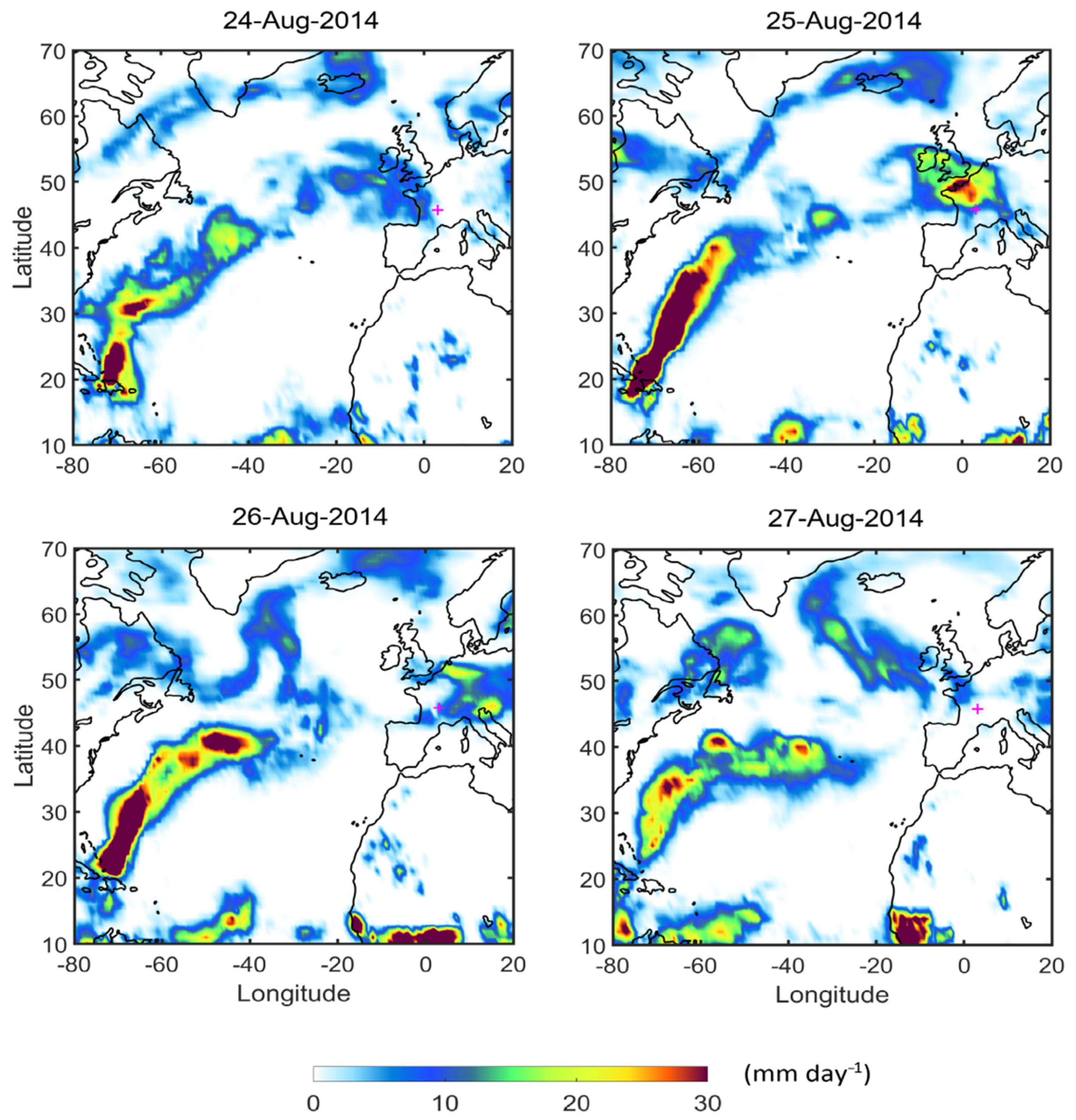
  • The large scale precipitation was provided by the Global Precipitation Climatology Project (GPCP [24]). GPCP is based on estimated precipitation by microwave polar-orbiting satellites and infrared imager onboard geostationary satellites. We used the product v1.3., which provides the mean daily precipitation at 1° × 1° resolution; and
  • The large scale horizontal cloud structures were provided by the Geostationary Operational Environmental Satellite (GOES 13). GOES 13 was launched in 2006 and took imagery in infrared and visible channels with a best resolution of 1 km at nadir [25]. We used the true color product over the North Atlantic (10° N–70° N, 80° W–20° E). True color is a daily mosaic in the visible channel.

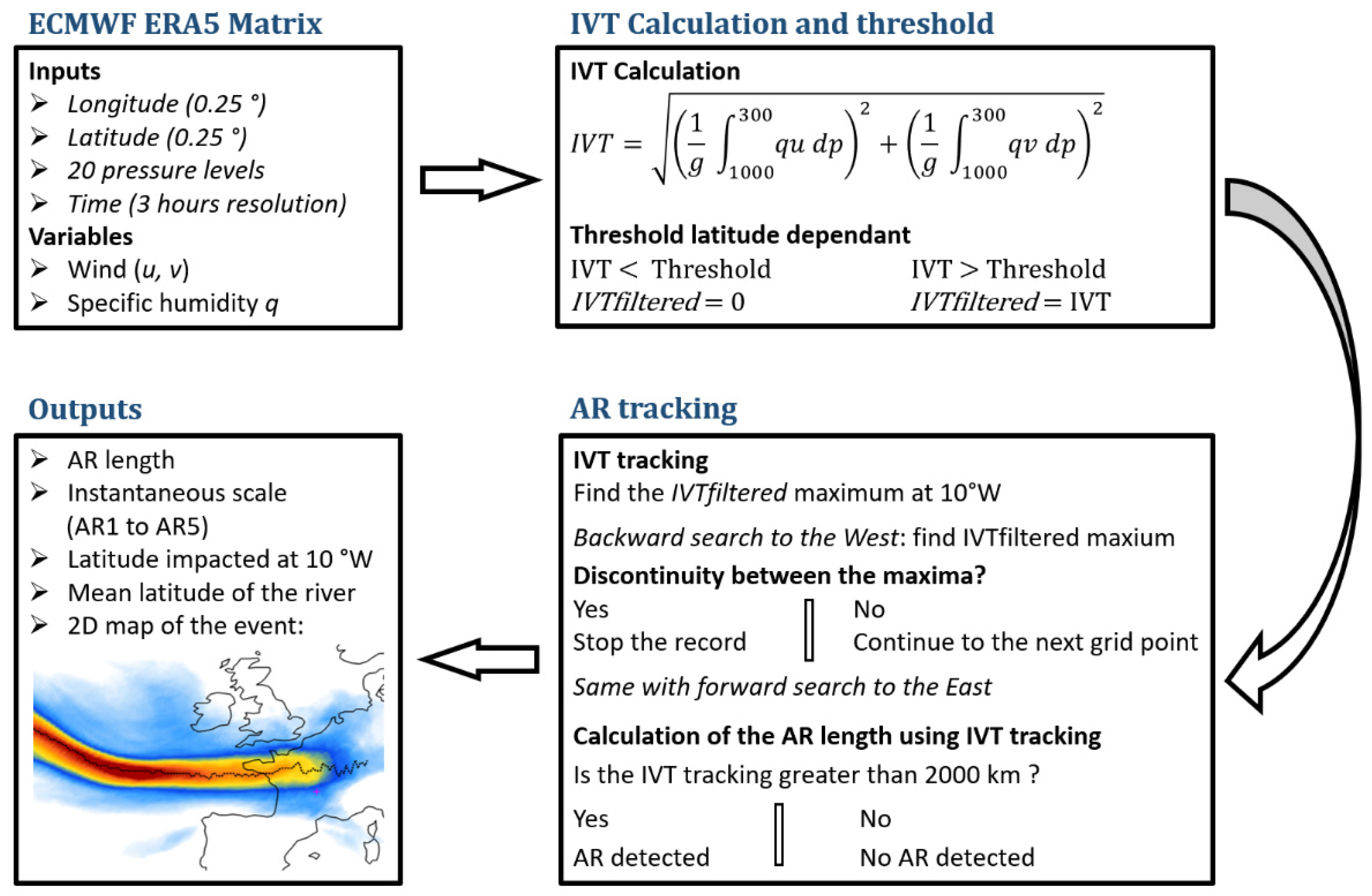
3. Methodology for Atmospheric Rivers Tracking: The ARiD (Atmospheric River Detector) Code

3.1. Integrated Vapor Transport and Threshold

Two parameters are commonly used to detect AR structure. The first is based on the IWV and the second on the IVT, which represents the magnitude of the horizontal water vapor flux vertically integrated between 1000 and 300 hPa as follows:
I V T = ( 1 g 1000 300 q u   d p ) ² + ( 1 g 1000 300 q v   d p ) ² ,
where q is the specific humidity (kg kg−1); u and v are the zonal and meridional components of wind (m s−1); g is the acceleration due to gravity (m s−2); and d p is the pressure difference between two adjacent pressure levels. The specific humidity and the wind components were averaged on the layer between two adjacent pressure levels.
Equation (1) indicates that IVT is calculated by vertical integration between 1000 and 300 hPa. Water vapor is rarely homogeneously distributed over this entire atmospheric layer. It is often concentrated in specific vertical layers of the atmosphere. If a strong vertical wind shear occurs in a dry area, the impact on the IVT will remain small. If the wind shear occurs in or near the maximum of water vapor, it could have an impact on the development of the atmospheric river and on the integrated vapor transport, but this is taken into account in the IVT calculation, which integrates wind and water vapor on every level. For example, Norris et al. [26] calculated the water vapor budget during an AR event over the Northeast Pacific. They neglected the second-order effects of vertical wind shear, considering that the impact at the hourly time scale was small and that the troposphere was nearly barotropic in their case study.
An AR is typically associated with an IWV greater than 2 cm coupled to horizontal wind greater than 12.5 m s−1 in the lower 2 km [27] or IVT greater than 250 kg m−1 s−1 [28]. The IWV was used initially because it was directly available from the satellite, however, this parameter is very sensible to the temperature, and so to the latitude. For these reasons, the use of IVT as a proxy for AR detection is now well-established.
To be considered as an atmospheric river, the IVT structure must be longer than 2000 km, with IVT values greater than a given threshold. Choosing a constant threshold for the IVT is very convenient, but it cannot represent an accurate characteristic as the mean value of IVT depends on both the season and the considered region. To solve this issue, some studies such as Rutz et al. [29] tried to determine a variable threshold for the IVT, depending on the latitude, in a given ocean basin.
Threshold values are often obtained using the 85th percentile of the IVT distribution, extracted from a climatology, like in Guan and Waliser [30] or Lavers and Villarini [13]. Some other studies use a constant threshold of 250 kg m−1 s−1 [31]. There is currently no consensus on how to define an IVT threshold to detect AR [32]. In the present study, we calculated the IVT from 1980 to 2020 at 00 and 12 UT with ECMWF ERA-5 at 10° W and from 20° N to 70° N. Then, we used the 85th percentile of the IVT distribution to calculate an IVT threshold that depends on the latitude. To avoid some threshold discontinuities with the latitude and to optimize computation time, a sinusoidal fit of the 85th percentile is used by the algorithm. The equation of the sinusoidal fit and the comparison between the real distribution and the sinusoidal fit are provided in the Supplementary Materials (Figure S1).

3.2. Atmospheric Rivers Tracking

To be considered as an AR, the IVT structure must be greater than the threshold values (depending on the location) in a continuous way of at least 2000 km. The ARiD code has been developed to identify AR structures, based on the following methodology:
  • Every grid point with an IVT less than the threshold value is set equal to 0;
  • Along 10° W, the latitude of the IVT maximum, if identified, is called maxλ. If no value above the IVT threshold is found, the record is stopped. If an AR exists only westward of 10° W, it will not be detected by ARiD. If more than one AR is present at 10° W at different latitudes, only the AR with the higher IVT will be identified, but this situation is rare;
  • A westward search is done, and the latitude of the IVT maximum along the new longitude maxλ+1 is found. If there is a discontinuity greater than 3° in latitude between the points maxλ and maxλ+1, the record is stopped;
  • The record continues until a discontinuity is found in the longitude (IVT less than the threshold), or in the latitude (more than 3° of latitude between two adjacent IVT maxima). A same forward search is performed to the east. The mean latitude λ of the AR is determined and gives us a mean size of the grid point; and
  • The number of recorded points is converted in kilometers. If the final length is greater than 2000 km, the time-step corresponds to an AR event.
A schematic overview of the methodology is given in Figure 1.

3.3. Precipitation Associated with AR

The link between AR situation and precipitation was established using the total precipitation ECMWF ERA5 parameter (with a 3 h temporal resolution) when a pixel (latitude, longitude) associates a detected AR (IVT) and a positive value of total precipitation at the same time step.
The part of precipitation related to AR is determined in the whole extracted region for each month from January 1980 to December 2020 by simply making the ratio between the monthly precipitation occurring during an AR and the accumulate precipitation the same month. Even if a coincidence between AR and precipitation is found, it does not mean that a causal link between them is established. Precipitation can also be related to very specific thermodynamic conditions (such as a high convective available potential energy, an unstable atmosphere, moisture recycling through evapotranspiration processes etc.), even in presence of ARs. This was not considered in this study.

3.4. Long Term Trend Estimation

The trends on the number of occurrences of AR and on the associated precipitation were simply estimated by linear regression on the 1980–2020 data series at a monthly frequency. The uncertainty of the trend is related to the statistical error of the slope, which represents the geophysical variability of the data. The Student’s law allows the estimation of the statistical error on the slope of the regression line by:
a 1 = σ ^ a 1 . t ( 1 ) / 2 n 2 ,
with
σ ^ a 1 = σ ^ x n   V ( x )
and
σ ^ x = 1 n 2 x ( t ) 2
where n is the number of measurements x with a sampling of one day; V ( x ) is the variance of the observation variable x ; and t ( 1 ) / 2 n 2 is the quantile of the Student’s t distribution, equal to 1.98 at 97.5% level of confidence.

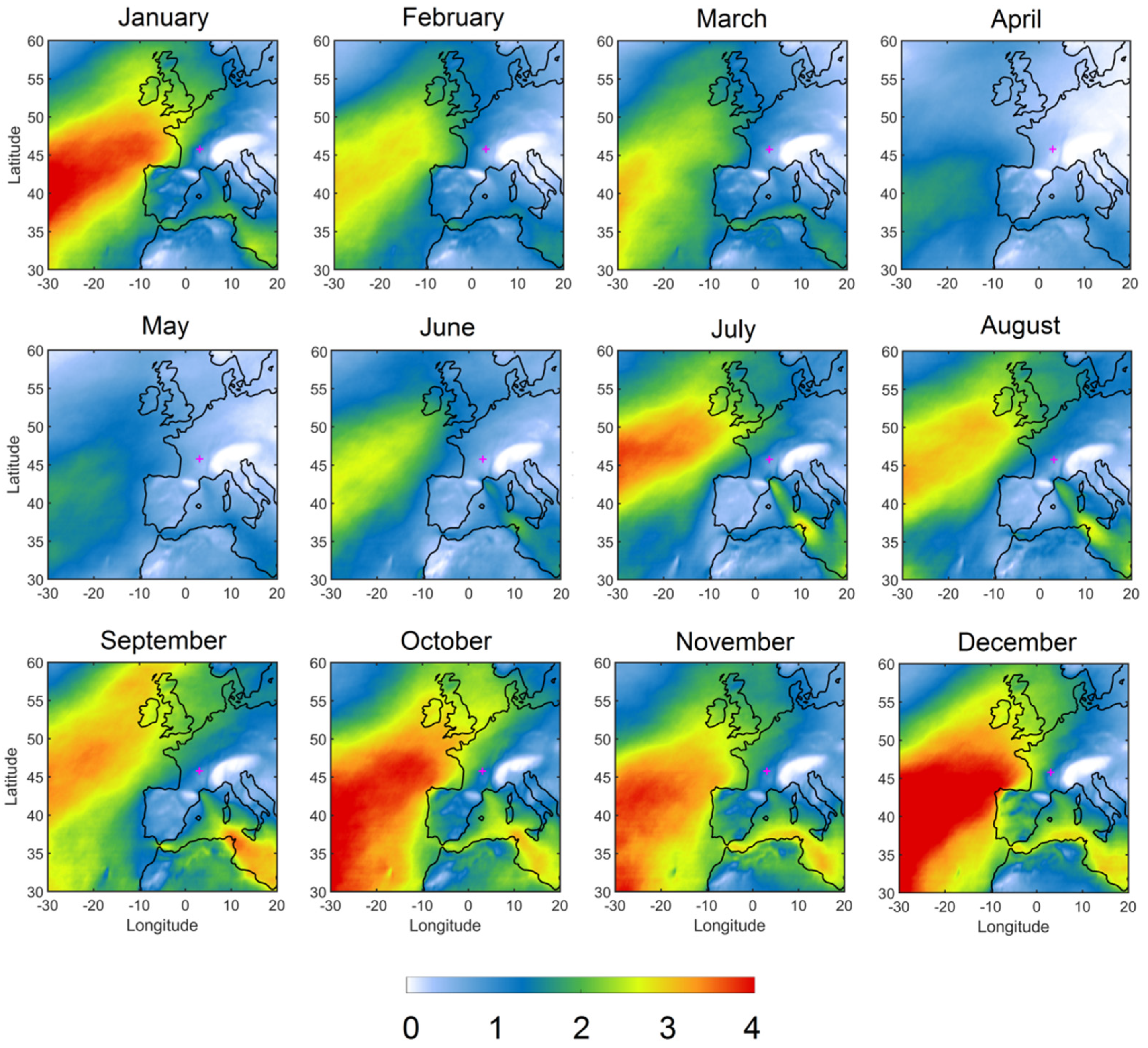
4. Climatology and Long-Term Trends

4.1. Localization of ARs

This section aims to determine the frequency of AR events and the average amount of precipitation that could be associated with AR in the 1980–2020 period.
Figure 2 presents the average number of AR days per month. The Atlantic area is the most impacted (maximum of four days per month), and AR occurrences decreased as the distance from the ocean increased. The October to January period is of most concern with an average of three AR days per month on the west coasts of the Iberian Peninsula, France, and British Islands. Interestingly, Mediterranean regions are also of concern.
The climatology covers the period 1980–2020, providing a significant sample of ARs. In the context of global warming and water vapor increase in the troposphere, one could expect an increase in the frequency of extreme events including AR. Nevertheless, we estimated the long-term trend using the method presented in Section 3.4.
For Clermont-Ferrand, we found −1.3 ± 2.0 h of AR decade−1. In a first approach, no significant tendency was thus observed. This was also the case for sites closer to the Atlantic Ocean such as Brest (48.44° N, 4.41° W, −0.5 ± 3.5 h of AR decade−1) and Bordeaux (44.83° N, 0.69° W, −0.9 ± 2.8 h of AR decade−1). Further studies on the evolution of AR frequency could be done using trends on other parameters such as the IVT distribution, multi-linear regression analysis, or by performing seasonal tendencies.

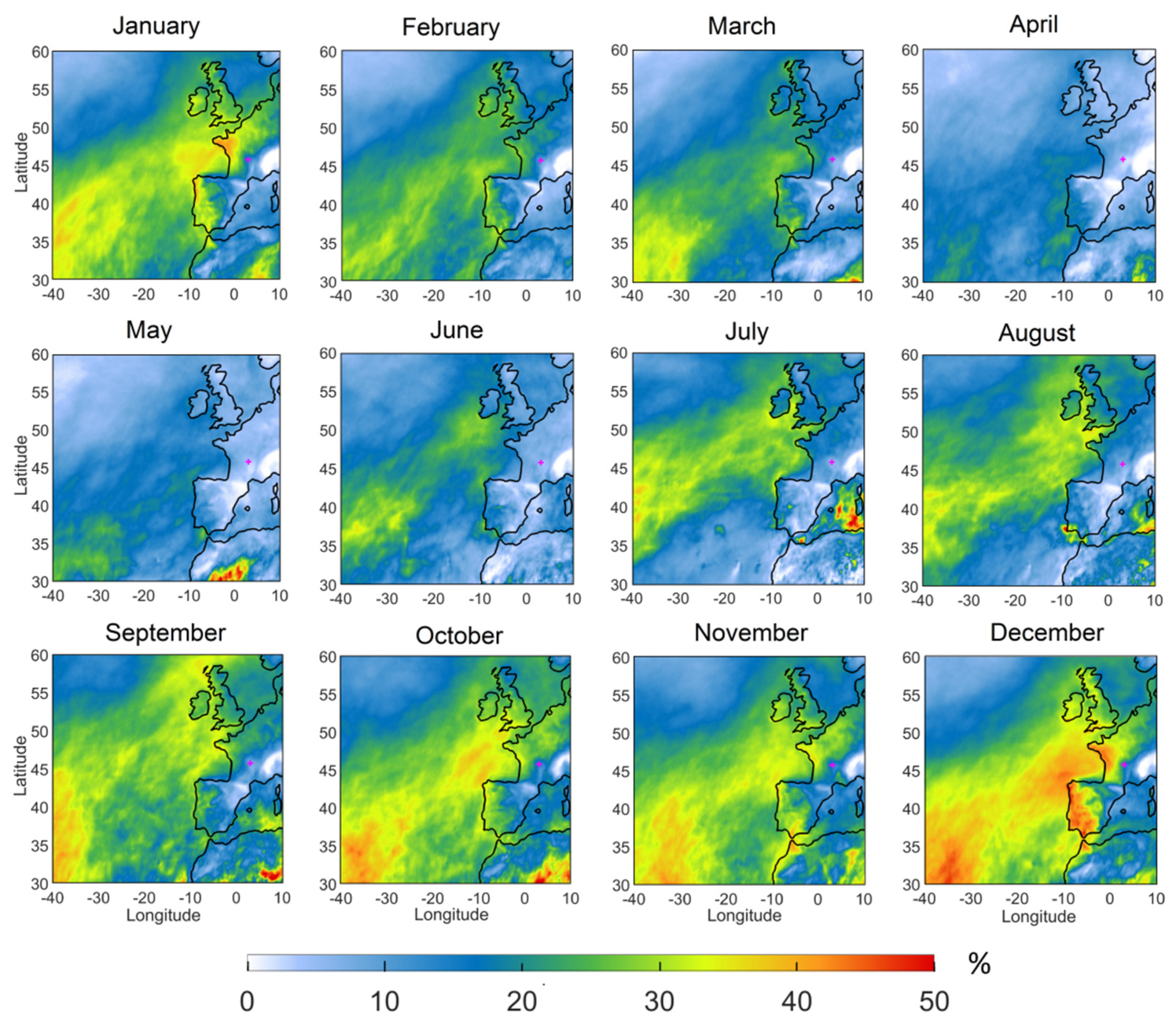
4.2. Precipitation Related to AR

While Figure 2 presents the localization of ARs, Figure 3 describes precipitation areas that coincided with detected ARs each month (following the methodology presented in Section 3.3). Our results are comparable to those obtained by Lavers and Villarini [34]. December and January were the months where the greatest AR contribution to rainfall was found, in agreement with AR occurrences found in Section 5.1.
The most impacted regions were the west coast of France and the Iberian Peninsula with part of the precipitation linked to AR presence greater than 40% in December, and greater than 30% from October to January. The spring and summer months (from April to August) had lower AR contribution due to the fewer numbers of extra-tropical cyclone occurrence.
Finally, AR contribution to precipitation reduces as the distance from the Atlantic Ocean increases because the phenomenon weakens when penetrating inland.

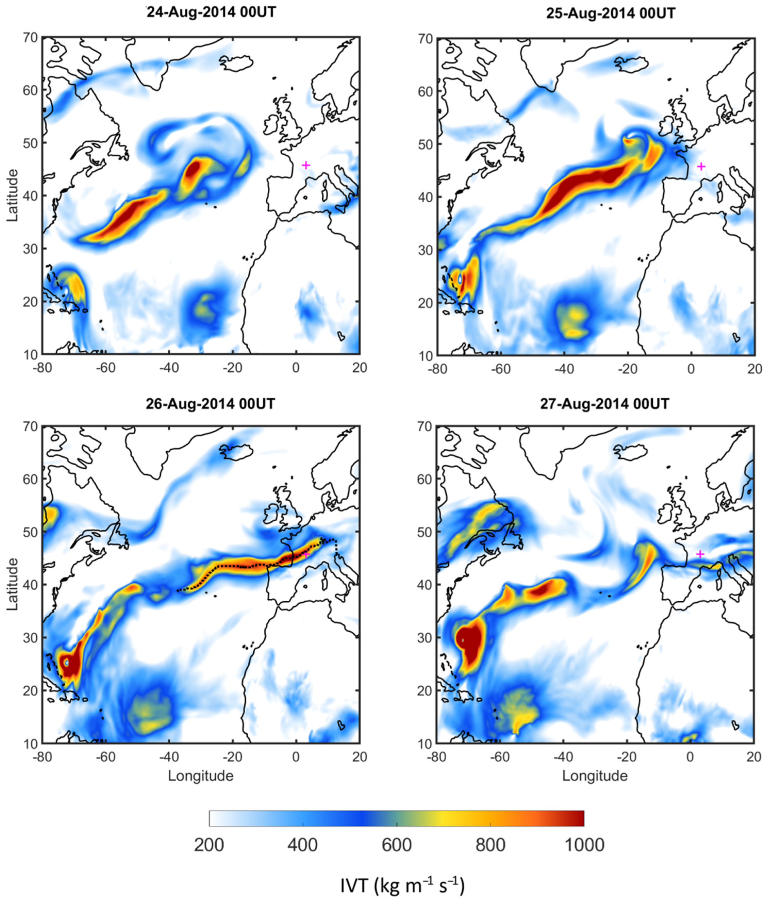
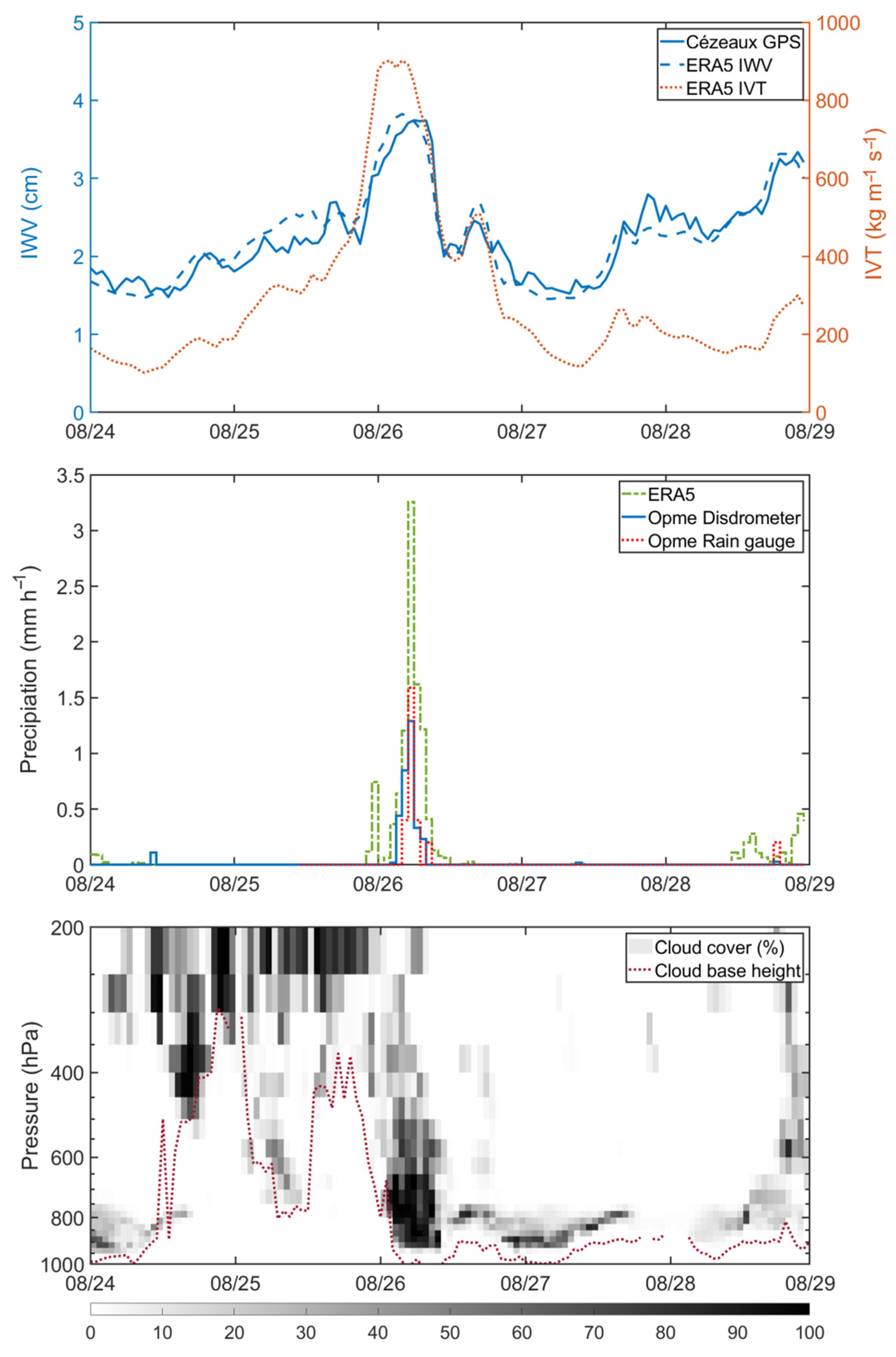
5. Case Study: 26 August 2014

While the aim of Section 4 was to estimate the frequency of AR events and the average amount of precipitation coinciding with AR events during the 1980–2020 period, the purpose of the Section 5 is to highlight a case study of AR that reached Clermont-Ferrand.

5.1. Conceptual Schemes of Jet Stream Dynamics and Stratosphere-Troposphere Exchange

The AR event of 26 August 2014 seems to be closely related to dynamic processes that are fundamental to understanding the evolution of this event. In this section, we present three of these concepts: ageostrophic circulations induced by jet stream, a reminder of the structure of extra-tropical cyclones, and the concept of PV.

5.1.1. Jet Streams and Ageostrophic Circulations

Jet streams constitute a major feature of the upper tropospheric dynamics. These narrow currents of strong horizontal wind are formed in response to the strong latitudinal gradients of temperature near frontal zones [35]. Wind speed is not constant along the jet stream and acceleration and deceleration zones are observed. These zones, called jet-streaks, are responsible for the ageostrophic wind circulation in the upper troposphere and lower stratosphere.
An entrance zone can be distinguished downstream of the jet streak, and an exit zone upstream. In the south entrance of a jet-streak, updrafts are observed in the troposphere while downdrafts are observed at the north entrance. An opposite circulation in the stratosphere is seen. In the north exit of the jet-streak, updrafts are observed and downdrafts in the south exit. In the same way as the entrance region, the air motion in the troposphere is associated with an opposite air motion in the stratosphere [36]. Such jet-streaks can be responsible for tropopause deformation and can even lead to tropopause folding [4,37,38]. The regions of downdrafts and updrafts can be responsible for perturbations in air fronts, triggering the cyclogenesis.

5.1.2. Extratropical Cyclones

Extratropical cyclones regulate the weather variability in mid-latitude regions. The air flows in such cyclones were first explained by the Bergen school at the beginning of the 20th century with two radically different air masses. The first one from polar origin will form the cold front, and the second one from tropical origin, the warm front. A small cyclonic disturbance (often due to jet streak) along the polar front will result in cold air advection (to the south) on the west side of the cyclone, and the advection of warm air (to the north) on the east side, leading to the typical structure of mid-latitude cyclones. Between the two fronts, a zone of enhanced moisture transport is found and is called the warm conveyor belt (WCB), which is characterized by a strong ascending trajectory [39]. Atmospheric rivers are usually sub regions of such WCBs [8].
The cold conveyor belt comes from the east or north and rotates anticlockwise due to the low-pressure circulation associated with the Coriolis force in the Northern Hemisphere. Usually, a dry intrusion of air coming from the upper troposphere is observed beyond the cold front and forms a cloud free zone.

5.1.3. PV and Stratospheric Intrusions

The thermal tropopause is defined as the lowest altitude at which the temperature lapse rate Γ = −∂T/∂z is lower than 2 K km−1 and the lapse rate averaged from this level to any other point in the next 2 km also has a Γ lower than 2 K km−1 [40]. This definition exhibits a vertical discontinuity in the static stability, which strongly increases in the stratosphere.
PV is one of the parameters regularly used to emphasize the height of the tropopause at mid-latitudes and to identify stratospheric intrusions [41]. With the conventional definition of PV (1 PVU = 10−6 m2 s−1 K kg−1), the tropopause was found to be relatively close to 2 PVU with a sharp decrease in the troposphere and high values in the stratosphere.
Hence, the notions of PV and thermal tropopause allow us to define the transition zone between the troposphere and the stratosphere, and PV values greater than 2 PVU in the troposphere can be a sign of stratospheric intrusion.
There are several processes that can lead to air mass exchange between the troposphere and the stratosphere [37]. The first one concerns the tropopause fold induced by the entrance and exit regions of a jet streak, which is described in the precedent part. The second one concerned cut off low, which could also be responsible for stratospheric intrusion [38]. Finally, intense convection can induce troposphere to stratosphere exchange by vertical flux, and stratosphere to troposphere exchange in the outlying regions [42].

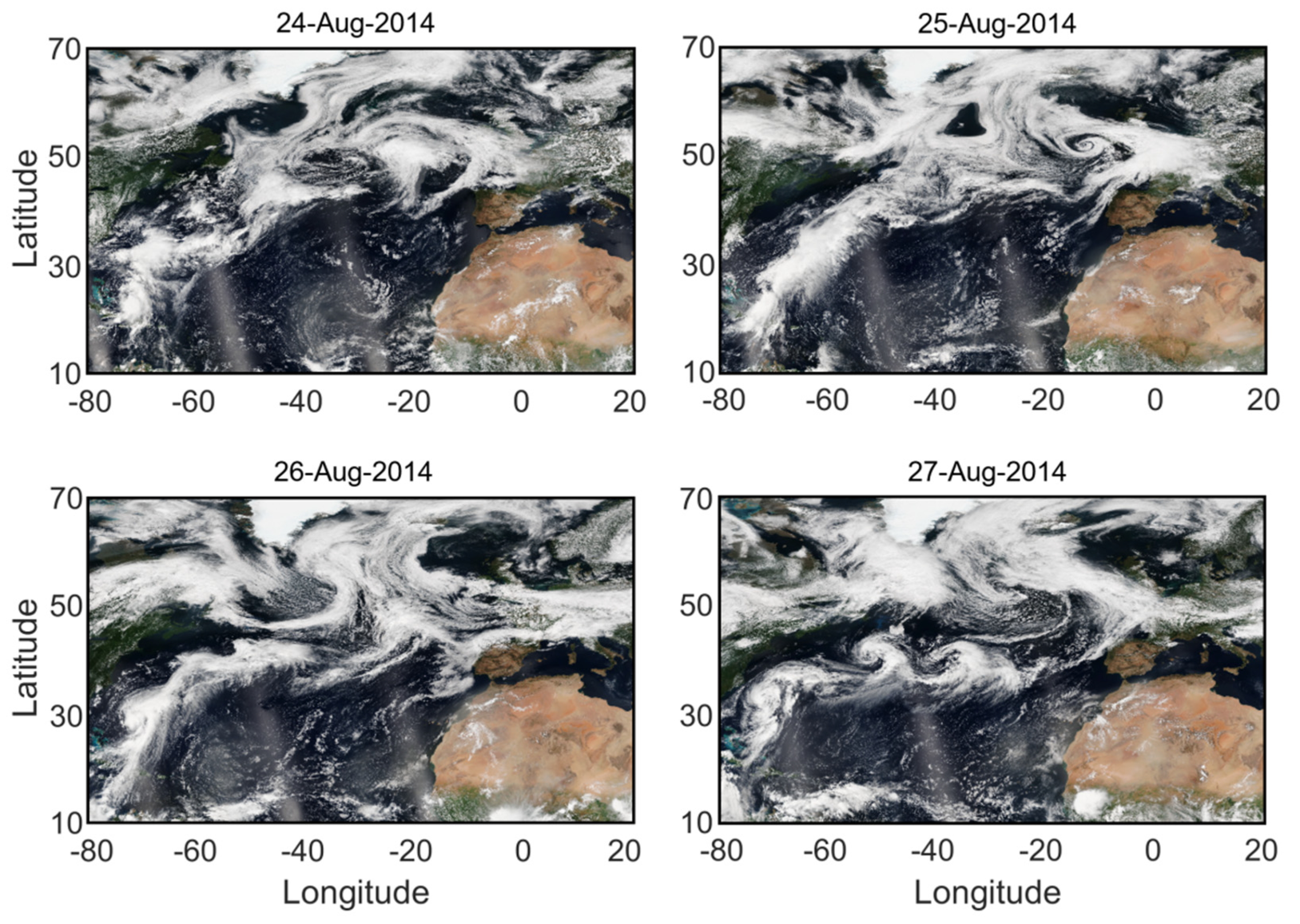
5.2. Synoptic Context and Temporal Evolution

The aim of this section is to detail the meteorological context that led to the formation and evolution of an AR detected by ARiD. The IVT patterns exhibited AR characteristics (no discontinuity, length greater than 2000 km) from 25 August at 07 UT (6200 km length) to 26 August at 23 UT. Figure 4 describes the successive stages of the AR event.
On 24 August, an extra-tropical cyclone started forming off the British Islands. Strong discontinued IVT patterns could be observed. The low-pressure system then advected to the west, driven by an intense jet stream.
The mid-latitude cyclone strengthened rapidly on 25 August and exhibited a minimum mean sea level pressure of 980 hPa at 07 UT. At this date, the IVT pattern crossed the west coast of France while it reached its maximum in magnitude (IVT greater than 1000 kg m−1 s−1) and in length (6200 km). The AR crossed France within a day, from 25 August (northwest) to 26 August (southwest).
On 26 August at 00 UT, the AR crossed over Clermont-Ferrand (pink cross on Figure 4) and then decreased in intensity as it penetrated inland. At this date, a tropical cyclone named Cristobal (Category 1 hurricane, 26 August at 00 UT) was located at the extreme west of the AR around 70° W/25° N [43]. A Category 1 hurricane corresponds to sustained wind speed greater than 32 m s−1 on the Saffir–Simpson scale.
The AR event ended south of Alps Mountain during the night between 26 and 27 August. The whole event seems to be closely related with the presence of an altitude jet stream and this interaction will be investigated in the following part.

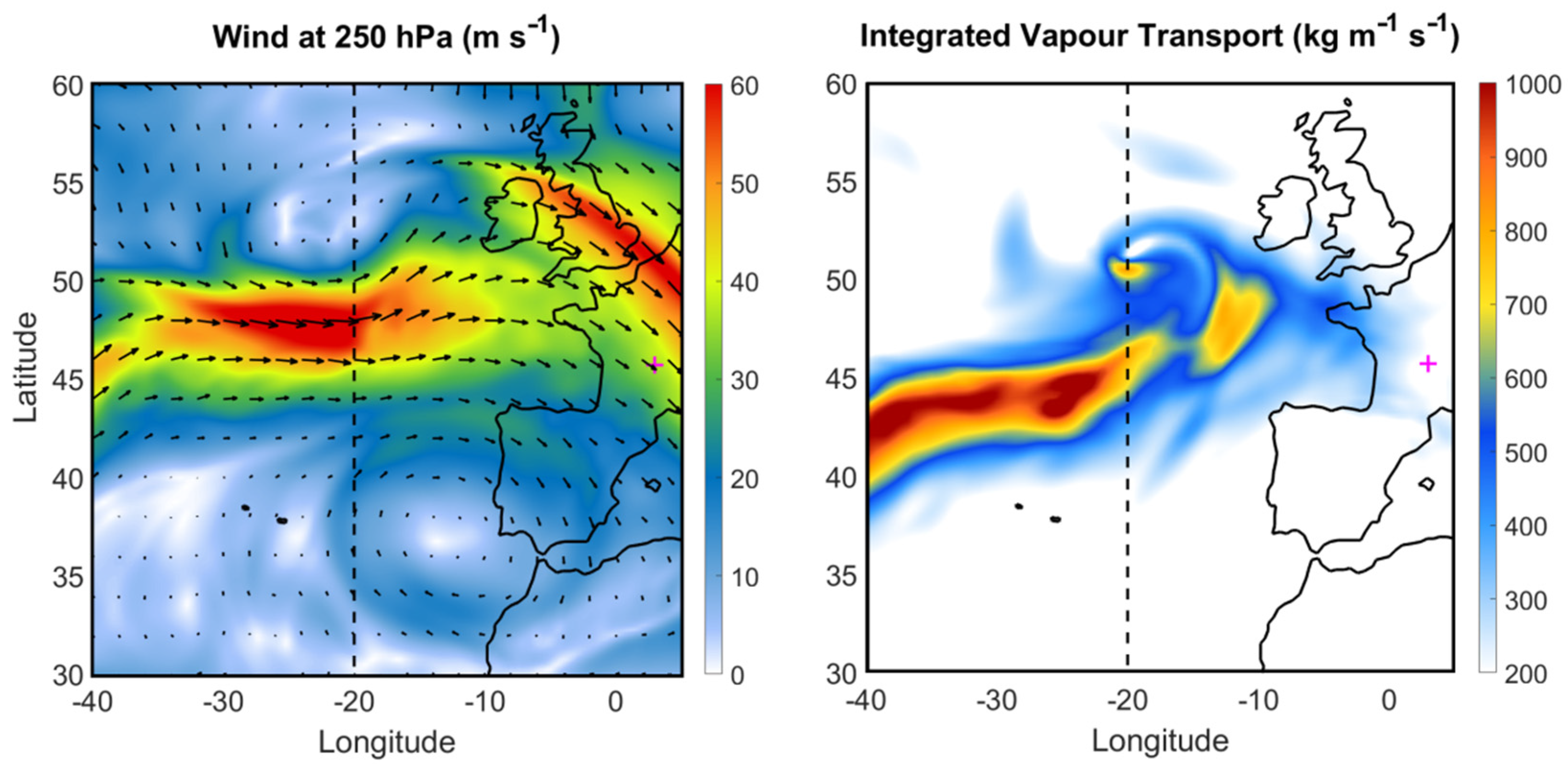
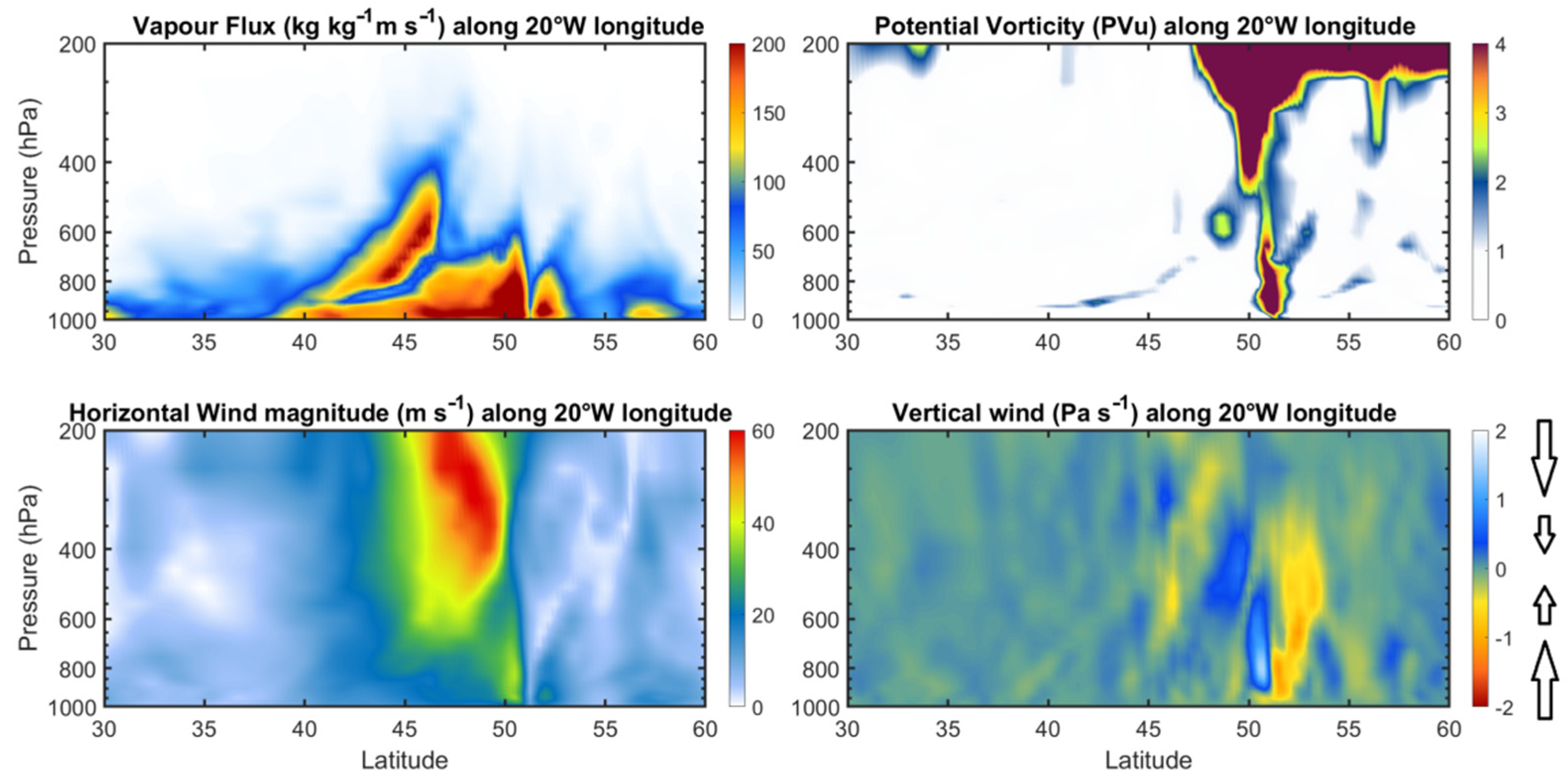
5.3. Atmospheric River, Jet Stream, and Tropopause Deformation

Section 5.2 detailed the AR evolution from its formation on 24 August 2014 to its end on 27 August 2014. The purpose of this section is to detail the phenomenon in the whole troposphere. Figure 5 presents the horizontal wind in the upper troposphere (250 hPa, corresponding to about 10 km) compared to the signature of the AR (IVT). A high-speed wind zone (more than 60 m s−1) occurred near 47° N between 35° W and 15° W. This zone presents the characteristics of a jet streak, with a west–east orientation. A second jet streak was located over England and France, in a northwest–southeast orientation. The AR was localized just southward and along the jet streaks. An extra-tropical cyclone formed off the British Islands, and the minimum mean sea level pressure at 985 hPa (not shown) corresponded to the dry region at 52° N.
The cross section, in dashed line in Figure 5, is performed in the exit zone of the first jet-streak at 20° W, where the ageostrophic wind circulations detailed in Section 5.1 are expected (Figure 6). Figure 6 shows the vertical cross sections of vapor flux, PV, horizontal wind, and vertical velocity.
In the water vapor flux cross section, the AR (between 800 hPa and 400 hPa) appeared to be lifted over a moist region and the dry zone at the center of the extra-tropical cyclone was clearly identifiable at 52° N. The PV cross section indicates a descent of the tropopause at 49° N with PV values greater than 4 PVU sinking until almost 500 hPa and another zone of high PV greater than 2.5 PVU coming from the ground between 50° N and 52° N and extending to 500 hPa.
The stratospheric intrusion observed around 49° N is probably due to a complex relationship between the jet-streak exit and the rapid cyclogenesis occurring at this date. Further studies including a mesoscale model will be needed to identify the role of latent heating in such rapid cyclogenesis and the interaction with the moisture provided by the AR. The following section will provide a 3D description of the water-vapor, liquid, and ice cloud structures obtained from satellite data.

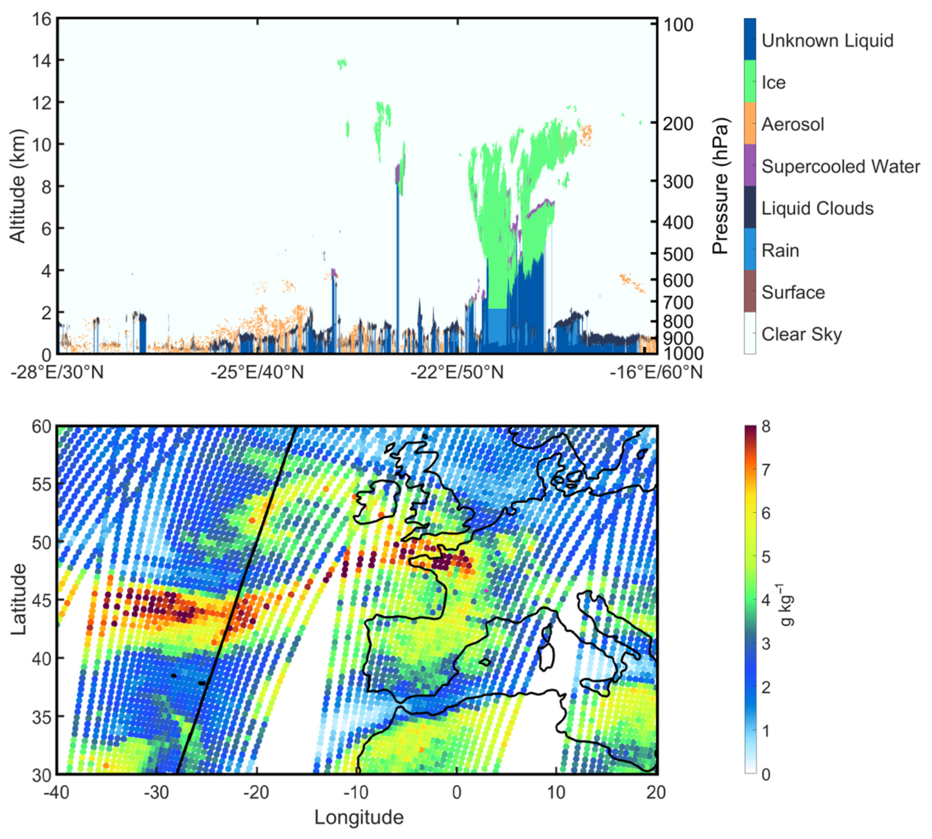
5.4. Vertical Description of Water Vapor and Liquid and Ice Clouds

Figure 7 presents a DARDAR cross section and satellite imagery of WVMR at 700 hPa provided by AIRS. The structure of the AR and of the extra-tropical cyclone appeared clearly on the satellite observations. A deep ice cloud structure was observed around 53° N from 4 km to 10 km with a super cooled liquid water layer at 7 km (Figure 7 top). Rain and liquid water were also present underneath the ice cloud in the cross-section.
Here, we are close to the region where two PV anomalies were observed in Figure 6. The morphology of this cloud structure can be associated with deep convection mechanism. This deep convection could be responsible for the PV anomaly observed close to ground until 500 hPa and the presence of ascending air motion (negative values of w in Pa s−1 in Figure 4 near 52–53° N). It is also interesting to note that no substantial cloud was observed in the cross section between 47° N and 51° N where the tropopause anomaly and the stratospheric intrusion were found.
Funatsu and Waugh [44] found a connection between PV intrusion and convection in the eastern tropical Pacific Ocean. We hypothesize that the upper PV anomaly triggered convection by causing an upward air motion ahead of the stratospheric intrusion. Further studies (latent heat release, isentropic inclinations etc.) would be necessary to confirm or refute this hypothesis for this case study.
The AR signature was observed on the AIRS WVMR map, with values reaching 8 g kg−1 at 700 hPa, corresponding to an altitude of about 3 km (Figure 7 bottom). The zone corresponding to the ice cloud presented more moderated values of about 6 g kg−1. A dry region (2 g kg−1) was also highlighted by AIRS where the stratospheric intrusion was localized (20° W and 47° N), although Figure 7 (bottom) corresponds to low-tropospheric levels. The upper troposphere levels confirm the presence of this dry region (not shown).

5.5. Clouds and Precipitation, Evolution until Central France

Figure 8 presents a mosaic of GOES satellite images in visible channels, covering the period of the AR event (24–27 August 2014). The extra-tropical cyclone is particularly visible on 25 August off the British Islands. A cloud free zone corresponding to a vast anticyclonic region was observable in all the pictures south of 40° N. The AR formed on 24 August and cloud structures followed the discontinued IVT patterns seen in Figure 2.
On 25 August, the extra-tropical cyclone was well developed, and a substantial cloudy region crossed Western Europe. The AR passed over France during the night between the 25 and the 26 August and a thin cloud region remained blocked in the north of the Pyrenees Mountains. Clouds were sparser on 26 August as the mid-latitude cyclone died in Eastern Europe.
Figure 9 presents the mean daily precipitation from GPCP v1.3 at the same dates as the GOES imagery, indicating that clouds developed near (around) the AR induced important rainfalls (more than 30 mm day−1).
Zones of intense precipitation in the Atlantic Ocean east of the United States (maximum on 25 and 26 August) can be attributed to the tropical cyclone Cristobal mentioned in Section 2.2. Intense precipitation was also found on 25 August in northern France (greater than 30 mm day−1) and can be associated with the AR.
These rain areas were advected eastward and precipitation was much more moderate (less than 10 mm day−1) at Clermont-Ferrand on 25 and 26 August. Two measurement points near Clermont-Ferrand, Cézeaux and Opme, separated by few kilometers were used to observe water vapor columns and precipitation during the AR event. Cézeaux is equipped with a GPS receiver for IWV measurement and Opme is equipped for rain measurements (rain gauge and disdrometer). Figure 10 presents the IWV, IVT, and rain rate series.
The IWV and IVT signals were intense when the AR crossed over the weather station (from 25 August at 21 UT to 26 August at 09 UT). The peak of IVT values were immediately followed by moderate precipitation retrieved by the disdrometer and the rain gauge (peak at 1.5 mm h−1 on 26 August at 00 UT). This peak of precipitation could also be seen by ERA5, but with much greater quantities. This difference in intensity can be explained by the resolution of the re-analysis, and the very local character of precipitation. It must be noticed that the correspondence between the peak in IWV and a subsequent precipitation event has already been documented with a statistical approach [45]. Finally, the cloud structures observed on the GOES imagery corresponded well to the ERA5 cross section, with high clouds on 25 August and sparse low clouds after 26 August.

6. Conclusions

Atmospheric rivers (AR) are important processes at the origin of many extreme precipitation and flood episodes in the mid-latitudes. First studied over the U.S. west coast, we proposed documenting the climatology established over the period 1980–2020 with ARiD, which uses a threshold based on the 85th percentile of the IVT distribution over the North Atlantic basin. We then detailed a case study of AR that occurred in France in August 2014 and reached Clermont-Ferrand located 400 km inland.
The first part of the study investigated AR climatology in Europe over the 1980–2020 period. The calculation of the tendencies in AR frequency indicates that the occurrence of the phenomenon remains stable, and no significant trend was found. The study in AR localization highlights that the coastal regions of Western Europe (west of France, Iberian Peninsula, and British Islands) are the most impacted by AR with an occurrence up to four days per month. The greatest contribution of AR to precipitation was found to occur in December and January in west France and west of the Iberian Peninsula with a contribution of about 40%.
Next, we detailed the evolution of an AR event detected by ARiD in August 2014. We found the evidence of a stratospheric intrusion in the PV signature and satellite imagery provided by DARDAR and AIRS helped us to hypothesize that this phenomenon could be linked to the rapid cyclogenesis of the extra-tropical cyclone that carried the AR. We observed the cloud formations (from GOES-13) and the precipitation structures (from GPCP) linked to the AR event at a regional scale. At the local scale, we found significant signatures in the IWV measures retrieved by GPS and precipitation was observed by disdrometer and rain gauge when the AR passed over the Clermont-Ferrand region. The precipitation occurred just after the observation of the IWV maximum. The observation of the case study emphasizes the need for mesoscale modeling to better understand the structure of AR and their interaction with the high troposphere. Some points remain unexplored such as the role of latent heating and the role of moisture provided by AR in rapid cyclogenesis.
Further studies in trends are needed to investigate the tendencies in the IVT distribution. AR occurrence is dependent on the season [30], and trend should take this characteristic in consideration. The climatology could also be extended to other regions of the world. For example, a study could be performed over the Indian Ocean of the Southern Hemisphere, which presents a different dynamical configuration, with southeasterly trade winds that flow in the lower troposphere and a westerly flow in the upper troposphere with the Maïdo Station [46] in Reunion Island as a measurement point. Threshold for AR detection should then be recalculated using the IVT distribution of the region of interest. A consensus on the determination of this threshold remains the greatest aim to pursue. Indeed, climatology on AR occurrence or on precipitation due to AR depends on the threshold used: the higher the threshold, the lower the number of ARs detected.

Supplementary Materials

The following is available online at https://www.mdpi.com/article/10.3390/atmos12081075/s1, Video S1: Animated Figure 5, details on the sinusoidal fit of IVT. Figure S1: The figure shows the good agreement between the real distribution of the 85th percentile of IVT (in black) and the sinusoidal fit (red circles).

Author Contributions

Conceptualization, J.-L.B., M.D. and B.D.; Methodology, J.-L.B. and B.D.; Software, B.D.; Validation, J.-L.B. and B.D.; Formal analysis, J.-L.B. and B.D.; Investigation, J.-L.B. and B.D.; Resources, J.-L.B. and N.M.; Data curation, J.-L.B. and N.M.; Writing—original draft preparation, J.-L.B. and B.D.; Writing—review and editing, J.-L.B., M.D., N.M. and B.D.; Visualization, J.-L.B. and B.D.; Supervision, J.-L.B.; Project administration, J.-L.B.; Funding acquisition, J.-L.B. and N.M. All authors have read and agreed to the published version of the manuscript.

Funding

The operation of the COPDD instrumental site was funded by CNRS, CNES, and Université Clermont Auvergne. The COPDD instrumentation also benefitted from the support of ACTRIS Research Infrastructure and FEDER European Regional funds.

Institutional Review Board Statement

Not applicable.

Informed Consent Statement

Not applicable.

Data Availability Statement

COPDD and DARDAR data can be found via AERIS and ICARE data services (https://www.aeris-data.fr/, accessed on 19 August 2021; https://www.icare.univ-lille.fr/, accessed on 19 August 2021). GOES images have been obtained with the NOAA view data exploration tool (https://www.nnvl.noaa.gov/view/#TRUE, accessed on 19 August 2021). We acknowledge the Climate Data Guide: GPCP (Daily): Global Precipitation Climatology Project (https://climatedataguide.ucar.edu/climate-data/gpcp-daily-global-precipitation-climatology-project, accessed on 19 August 2021). AIRS project (2019), Aqua/AIRS L2 Standard Physical Retrieval (AIRS+AMSU) V7.0, Greenbelt, MD, USA, Goddard Earth Sciences Data and Information Services Center (GES DISC), 10.5067/URTYDAGTM548.ERA5 variables were provided by the ECMWF data portal (https://apps.ecmwf.int/datasets/, accessed on 19 August 2021).

Acknowledgments

We acknowledge the technical and scientific staff of OPGC and LaMP for helpful discussions and data management.

Conflicts of Interest

The authors declare no conflict of interest.

References

  1. Hodnebrog, Ø.; Myhre, G.; Samset, B.H.; Alterskjær, K.; Andrews, T.; Boucher, O.; Faluvegi, G.; Fläschner, D.; Forster, P.M.; Kasoar, M.; et al. Water Vapour Adjustments and Responses Differ between Climate Drivers. Atmos. Chem. Phys. 2019, 19, 12887–12899. [Google Scholar] [CrossRef] [Green Version]
  2. Voigt, A.; Bony, S.; Dufresne, J.-L.; Stevens, B. The Radiative Impact of Clouds on the Shift of the Intertropical Convergence Zone. Geophys. Res. Lett. 2014, 41, 4308–4315. [Google Scholar] [CrossRef] [Green Version]
  3. O’Gorman, P.A.; Muller, C.J. How Closely Do Changes in Surface and Column Water Vapor Follow Clausius–Clapeyron Scaling in Climate Change Simulations? Environ. Res. Lett. 2010, 5, 025207. [Google Scholar] [CrossRef]
  4. Baray, J.L.; Pointin, Y.; Van Baelen, J.; Lothon, M.; Campistron, B.; Cammas, J.P.; Masson, O.; Colomb, A.; Hervier, C.; Bezombes, Y.; et al. Case Study and Climatological Analysis of Upper-Tropospheric Jet Stream and Stratosphere-Troposphere Exchanges Using VHF Profilers and Radionuclide Measurements in France. J. Appl. Meteorol. Climatol. 2017, 56, 3081–3097. [Google Scholar] [CrossRef]
  5. Sherwood, S.C.; Roca, R.; Weckwerth, T.M.; Andronova, N.G. Tropospheric Water Vapor, Convection, and Climate. Rev. Geophys. 2010, 48, RG2001. [Google Scholar] [CrossRef] [Green Version]
  6. Zhu, Y.; Newell, R.E. A Proposed Algorithm for Moisture Fluxes from Atmospheric Rivers. Mon. Weather Rev. 1998, 126, 725. [Google Scholar] [CrossRef]
  7. Knippertz, P.; Wernli, H. A Lagrangian Climatology of Tropical Moisture Exports to the Northern Hemispheric Extratropics. J. Clim. 2010, 23, 987–1003. [Google Scholar] [CrossRef] [Green Version]
  8. Ralph, F.M.; Cannon, F.; Tallapragada, V.; Davis, C.A.; Doyle, J.D.; Pappenberger, F.; Subramanian, A.; Wilson, A.M.; Lavers, D.A.; Reynolds, C.A.; et al. West Coast Forecast Challenges and Development of Atmospheric River Reconnaissance. Bull. Am. Meteorol. Soc. 2020, 101, E1357–E1377. [Google Scholar] [CrossRef]
  9. Behringer, D.; Chiao, S. Numerical Investigations of Atmospheric Rivers and the Rain Shadow over the Santa Clara Valley. Atmosphere 2019, 10, 114. [Google Scholar] [CrossRef] [Green Version]
  10. Bozkurt, D.; Rondanelli, R.; Marín, J.C.; Garreaud, R. Foehn Event Triggered by an Atmospheric River Underlies Record-Setting Temperature Along Continental Antarctica. J. Geophys. Res. Atmos. 2018, 123, 3871–3892. [Google Scholar] [CrossRef]
  11. Mattingly, K.S.; Mote, T.L.; Fettweis, X. Atmospheric River Impacts on Greenland Ice Sheet Surface Mass Balance. J. Geophys. Res. Atmos. 2018, 123, 8538–8560. [Google Scholar] [CrossRef] [Green Version]
  12. Douluri, D.L.; Chakraborty, A. Assessment of WRF-ARW Model Parameterization Schemes for Extreme Heavy Precipitation Events Associated with Atmospheric Rivers over West Coast of India. Atmos. Res. 2021, 249, 105330. [Google Scholar] [CrossRef]
  13. Lavers, D.A.; Villarini, G. The Nexus between Atmospheric Rivers and Extreme Precipitation across Europe. Geophys. Res. Lett. 2013, 40, 3259–3264. [Google Scholar] [CrossRef]
  14. Pasquier, J.T.; Pfahl, S.; Grams, C.M. Modulation of Atmospheric River Occurrence and Associated Precipitation Extremes in the North Atlantic Region by European Weather Regimes. Geophys. Res. Lett. 2019, 46, 1014–1023. [Google Scholar] [CrossRef] [Green Version]
  15. Ramos, A.M.; Trigo, R.M.; Tomé, R.; Liberato, M.L.R. Impacts of Atmospheric Rivers in Extreme Precipitation on the European Macaronesian Islands. Atmosphere 2018, 9, 325. [Google Scholar] [CrossRef] [Green Version]
  16. Hoffmann, L.; Günther, G.; Li, D.; Stein, O.; Wu, X.; Griessbach, S.; Heng, Y.; Konopka, P.; Müller, R.; Vogel, B.; et al. From ERA-Interim to ERA5: The Considerable Impact of ECMWF’s next-Generation Reanalysis on Lagrangian Transport Simulations. Atmos. Chem. Phys. 2019, 19, 3097–3124. [Google Scholar] [CrossRef] [Green Version]
  17. Baray, J.-L.; Deguillaume, L.; Colomb, A.; Sellegri, K.; Freney, E.; Rose, C.; Van Baelen, J.; Pichon, J.-M.; Picard, D.; Fréville, P.; et al. Cézeaux-Aulnat-Opme-Puy De Dôme: A Multi-Site for the Long-Term Survey of the Tropospheric Composition and Climate Change. Atmos. Meas. Tech. 2020, 13, 3413–3445. [Google Scholar] [CrossRef]
  18. Bevis, M.; Businger, S.; Herring, T.A.; Rocken, C.; Anthes, R.A.; Ware, R.H. GPS Meteorology: Remote Sensing of Atmospheric Water Vapor Using the Global Positioning System. J. Geophys. Res. Atmos. 1992, 97, 15787–15801. [Google Scholar] [CrossRef]
  19. Bock, O.; Bosser, P.; Bourcy, T.; David, L.; Goutail, F.; Hoareau, C.; Keckhut, P.; Legain, D.; Pazmino, A.; Pelon, J.; et al. Accuracy Assessment of Water Vapour Measurements from in Situ and Remote Sensing Techniques during the DEMEVAP 2011 Campaign at OHP. Atmos. Meas. Tech. 2013, 6, 2777–2802. [Google Scholar] [CrossRef] [Green Version]
  20. Raupach, T.H.; Berne, A. Correction of Raindrop Size Distributions Measured by Parsivel Disdrometers, Using a Two-Dimensional Video Disdrometer as a Reference. Atmos. Meas. Tech. 2015, 8, 343–365. [Google Scholar] [CrossRef] [Green Version]
  21. Parkinson, C.L. Aqua: An Earth-Observing Satellite Mission to Examine Water and Other Climate Variables. IEEE Trans. Geosci. Remote Sens. 2003, 41, 173–183. [Google Scholar] [CrossRef]
  22. Ceccaldi, M.; Delanoë, J.; Hogan, R.J.; Pounder, N.L.; Protat, A.; Pelon, J. From CloudSat-CALIPSO to EarthCare: Evolution of the DARDAR Cloud Classification and Its Comparison to Airborne Radar-Lidar Observations. J. Geophys. Res. Atmos. 2013, 118, 7962–7981. [Google Scholar] [CrossRef]
  23. Delanoë, J.; Hogan, R.J. Combined CloudSat-CALIPSO-MODIS Retrievals of the Properties of Ice Clouds. J. Geophys. Res. Atmos. 2010, 115. [Google Scholar] [CrossRef] [Green Version]
  24. Huffman, G.J.; Adler, R.F.; Morrissey, M.M.; Bolvin, D.T.; Curtis, S.; Joyce, R.; McGavock, B.; Susskind, J. Global Precipitation at One-Degree Daily Resolution from Multisatellite Observations. J. Hydrometeorol. 2001, 2, 36. [Google Scholar] [CrossRef] [Green Version]
  25. Hillger, D.W.; Schmit, T.J. Observing Systems: The GOES-13 Science Test: A Synopsis. Bull. Am. Meteorol. Soc. 2009, 90, 592–597. [Google Scholar] [CrossRef]
  26. Norris, J.R.; Ralph, F.M.; Demirdjian, R.; Cannon, F.; Blomquist, B.; Fairall, C.W.; Spackman, J.R.; Tanelli, S.; Waliser, D.E. The Observed Water Vapor Budget in an Atmospheric River over the Northeast Pacific. J. Hydrometeorol. 2020, 21, 2655–2673. [Google Scholar] [CrossRef]
  27. Ralph, F.M.; Dettinger, M.D. Storms, Floods, and the Science of Atmospheric Rivers. EOS Trans. Am. Geophys. Union 2011, 92, 265–266. [Google Scholar] [CrossRef] [Green Version]
  28. Rutz, J.J.; Steenburgh, W.J.; Ralph, F.M. Climatological Characteristics of Atmospheric Rivers and Their Inland Penetration over the Western United States. Mon. Weather Rev. 2014, 142, 905–921. [Google Scholar] [CrossRef]
  29. Rutz, J.J.; Shields, C.A.; Lora, J.M.; Payne, A.E.; Guan, B.; Ullrich, P.; O’Brien, T.; Leung, L.R.; Ralph, F.M.; Wehner, M.; et al. The Atmospheric River Tracking Method Intercomparison Project (ARTMIP): Quantifying Uncertainties in Atmospheric River Climatology. J. Geophys. Res. Atmos. 2019, 124, 13,777–13,802. [Google Scholar] [CrossRef]
  30. Guan, B.; Waliser, D.E. Detection of Atmospheric Rivers: Evaluation and Application of an Algorithm for Global Studies. J. Geophys. Res. Atmos. 2015, 120, 12514–12535. [Google Scholar] [CrossRef]
  31. Rutz, J.J.; Steenburgh, W.J.; Ralph, F.M. The Inland Penetration of Atmospheric Rivers over Western North America: A Lagrangian Analysis. Mon. Weather Rev. 2015, 143, 1924–1944. [Google Scholar] [CrossRef]
  32. Lora, J.M.; Shields, C.A.; Rutz, J.J. Consensus and Disagreement in Atmospheric River Detection: ARTMIP Global Catalogues. Geophys. Res. Lett. 2020, 47, e2020GL089302. [Google Scholar] [CrossRef]
  33. Ralph, F.M.; Rutz, J.J.; Cordeira, J.M.; Dettinger, M.D.; Anderson, M.; Reynolds, D.; Schick, L.J.; Smallcomb, C. A Scale to Characterize the Strength and Impacts of Atmospheric Rivers. Bull. Am. Meteorol. Soc. 2019, 100, 269–289. [Google Scholar] [CrossRef]
  34. Lavers, D.A.; Villarini, G. The Contribution of Atmospheric Rivers to Precipitation in Europe and the United States. J. Hydrol. 2015, 522, 382–390. [Google Scholar] [CrossRef]
  35. Palmen, E.; Newton, C.W. A Study of the Mean Wind and Temperature Distributionin the Vicinity of the Polar Front in Winter. J. Meteorol. 1948, 5, 220–223. [Google Scholar] [CrossRef] [Green Version]
  36. Mattocks, C.; Bleck, R. Jet Streak Dynamics and Geostrophic Adjustment Processes during the Initial Stages of Lee Cyclogenesis. Mon. Weather Rev. 1986, 114, 2033–2056. [Google Scholar] [CrossRef] [Green Version]
  37. Holton, J.R.; Haynes, P.H.; McIntyre, M.E.; Douglass, A.R.; Rood, R.B.; Pfister, L. Stratosphere-Troposphere Exchange. Rev. Geophys. 1995, 33, 403–439. [Google Scholar] [CrossRef]
  38. Sprenger, M.; Wernli, H.; Bourqui, M. Stratosphere Troposphere Exchange and Its Relation to Potential Vorticity Streamers and Cutoffs near the Extratropical Tropopause. J. Atmos. Sci. 2007, 64, 1587. [Google Scholar] [CrossRef]
  39. Boettcher, M.; Schäfler, A.; Sprenger, M.; Sodemann, H.; Kaufmann, S.; Voigt, C.; Schlager, H.; Summa, D.; Di Girolamo, P.; Nerini, D.; et al. Lagrangian Matches between Observations from Aircraft, Lidar and Radar in a Warm Conveyor Belt Crossing Orography. Atmos. Chem. Phys. 2021, 21, 5477–5498. [Google Scholar] [CrossRef]
  40. Gettelman, A.; Hoor, P.; Pan, L.L.; Randel, W.J.; Hegglin, M.I.; Birner, T. The Extratropicam Upper Troposphere and Lower Stratosphere. Rev. Geophys. 2011, 49. [Google Scholar] [CrossRef] [Green Version]
  41. Hoskins, B.J.; McIntyre, M.E.; Robertson, A.W. On the Use and Significance of Isentropic Potential Vorticity Maps. Q. J. R. Meteorol. Soc. 1985, 111, 877–946. [Google Scholar] [CrossRef]
  42. Homeyer, C.R.; Bowman, K.P.; Pan, L.L.; Zondlo, M.A.; Bresch, J.F. Convective Injection into Stratospheric Intrusions. J. Geophys. Res. Atmos. 2011, 116, D23304. [Google Scholar] [CrossRef] [Green Version]
  43. Nguyen, L.T.; Rogers, R.F.; Reasor, P.D. Thermodynamic and Kinematic Influences on Precipitation Symmetry in Sheared Tropical Cyclones: Bertha and Cristobal (2014). Mon. Weather Rev. 2017, 145, 4423–4446. [Google Scholar] [CrossRef]
  44. Funatsu, B.M.; Waugh, D.W. Connections between Potential Vorticity Intrusions and Convection in the Eastern Tropical Pacific. J. Atmos. Sci. 2008, 65, 987. [Google Scholar] [CrossRef]
  45. Labbouz, L.; Van Baelen, J.; Duroure, C. Investigation of the Links between Water Vapor Field Evolution and Rain Rate Based on 5  Years of Measurements at a Midlatitude Site. Geophys. Res. Lett. 2015, 42, 9538–9545. [Google Scholar] [CrossRef]
  46. Baray, J.-L.; Courcoux, Y.; Keckhut, P.; Portafaix, T.; Tulet, P.; Cammas, J.-P.; Hauchecorne, A.; Godin Beekmann, S.; De Mazière, M.; Hermans, C.; et al. Maïdo Observatory: A New High-Altitude Station Facility at Reunion Island (21° S, 55° E) for Long-Term Atmospheric Remote Sensing and in Situ Measurements. Atmos. Meas. Tech. 2013, 6, 2865–2877. [Google Scholar] [CrossRef] [Green Version]
Figure 1. Schematic overview of ARiD. AR1 to AR5 refer to the recently created atmospheric river intensity and impact scale [33].
Atmosphere 12 01075 g001
Figure 2. Average number of AR days each month over the period 1980–2020 from January (top left) to December (bottom right). The location of Clermont-Ferrand is marked by a pink cross.
Atmosphere 12 01075 g002
Figure 3. Monthly percentage of precipitation linked to the presence of AR over the period 1980–2020 from January (top left) to December (bottom right). The location of Clermont-Ferrand is marked by a pink cross.
Atmosphere 12 01075 g003
Figure 4. ECMWF ERA5 IVT maps during the atmospheric river event from 24 (top left) to 27 August 2014 (bottom right). The location of Clermont-Ferrand is marked by a pink cross.
Atmosphere 12 01075 g004
Figure 5. ECMWF ERA5 horizontal wind on the 250 hPa pressure level (left) and IVT maps (right) on 25 August 2014 at 00 UT. The dashed line represents the cross sections presented in Figure 4. The location of Clermont-Ferrand is marked by a pink cross. An animated version of this figure covering the 24–28 August period is provided as a video in the Supplementary Materials.
Atmosphere 12 01075 g005
Figure 6. ECMWF ERA5 Cross sections along 20° W longitude (25 August 2014 at 00 UT) of water vapor flux (kg kg-1 m s−1, top left), PV (PVU, top right), horizontal wind (m s−1, bottom left), and vertical wind (Pa s−1, the correspondence between sign, colors, and direction of the vertical wind is given with the color bar, bottom right).
Atmosphere 12 01075 g006
Figure 7. DARDAR simplified characterization on 25 August 2014 at 04 UT (top), and WVMR retrieved by AIRS at 700 hPa on 25 August from 00 to 06 UT (bottom). The black line represents the localization of the DARDAR cross-section.
Atmosphere 12 01075 g007
Figure 8. GOES mosaic in visible channels covering the different stages of the AR from 24 (top left) to 27 August 2014 (bottom right).
Atmosphere 12 01075 g008
Figure 9. Daily precipitation estimates from GPCP v1.3 from 24 (top left) to 27 August 2014 (bottom right). The location of Clermont-Ferrand is marked by a pink cross.
Atmosphere 12 01075 g009
Figure 10. IVT and IWV retrieved by ERA5 and IWV retrieved by GPS at Cézeaux (top); hourly precipitation accumulation from ERA5, disdrometer and rain gauge at Opme (middle); cloud cover and cloud base height (ECMWF ERA5, bottom). The interpolation location of ERA5 is 3° E, 45.75° N.
Atmosphere 12 01075 g010
Publisher’s Note: MDPI stays neutral with regard to jurisdictional claims in published maps and institutional affiliations.

