Comparison of CMIP5 and CMIP6 Multi-Model Ensemble for Precipitation Downscaling Results and Observational Data: The Case of Hanjiang River Basin

Abstract

Evaluating global climate model (GCM) outputs is essential for accurately simulating future hydrological cycles using hydrological models. The GCM multi-model ensemble (MME) precipitation simulations of the Climate Model Intercomparison Project Phases 5 and 6 (CMIP5 and CMIP6, respectively) were spatially and temporally downscaled according to a multi-site statistical downscaling method for the Hanjiang River Basin (HRB), China. Downscaled precipitation accuracy was assessed using data collected from 14 meteorological stations in the HRB. The spatial performances, temporal performances, and seasonal variations of the downscaled CMIP5-MME and CMIP6-MME were evaluated and compared with observed data from 1970–2005. We found that the multi-site downscaling method accurately downscaled the CMIP5-MME and CMIP6-MME precipitation simulations. The downscaled precipitation of CMIP5-MME and CMIP6-MME captured the spatial pattern, temporal pattern, and seasonal variations; however, precipitation was slightly overestimated in the western and central HRB and precipitation was underestimated in the eastern HRB. The precipitation simulation ability of the downscaled CMIP6-MME relative to the downscaled CMIP5-MME improved because of reduced biases. The downscaled CMIP6-MME better simulated precipitation for most stations compared to the downscaled CMIP5-MME in all seasons except for summer. Both the downscaled CMIP5-MME and CMIP6-MME exhibit poor performance in simulating rainy days in the HRB.

1. Introduction

Over the past several decades, climate change, as a vital component of the changing environment, has impacted the hydrological cycle process by varying degrees, leading to hydrological effects [1]. Precipitation is a key component of the climate system and a necessary condition for the formation and transformation of runoff [2]. Precipitation changes caused by climate change alter the original rainfall-runoff relationship in the hydrological cycle [1,3,4,5]. Climate change and the resulting precipitation variability substantially impact water resource shortages, distributions, and flood risk uncertainties. Assessing hydrological responses to future climate changes is essential for reducing flooding risks, managing water resources, and addressing hydroclimatic variabilities [6].

The most common approach to investigating the impacts of climate change on runoff is hydrological modeling [5]. The accuracy of precipitation, used as an input for hydrological models, affects the reliability of runoff prediction results. Global climate models (GCMs), which are developed by various modeling groups worldwide under the aegis of the Coupled Model Intercomparison Project (CMIP), are widely used to study the precipitation evolution of past, present, and future climate changes arising from natural, unforced variability or in response to climate change radiative forcing in a multi-model context [7,8]. Because of the spatial and temporal inadequacies of GCMs, downscaling methods have an essential role in increasing the effectiveness of GCMs at regional and local scales. Dynamical and statistical downscaling methodologies have previously been applied to downscale GCM outputs. The dynamical downscaling method employs regional climate models to generate regional-scale climate variables, using GCM outputs as the boundary conditions. Statistical downscaling methods are typically categorized into three groups—weather typing, stochastic generators, and regression-based approaches [9]. Compared with the dynamical downscaling method, the calculations required for statistical downscaling are fewer in number and easier to apply, which conserves both time and effort. Therefore, the statistical downscaling method is favored by experts worldwide [2,10]. The single-station weather generator statistical downscaling method can only produce climate change scenarios for a single point or for independent scenarios at several points [11]. Therefore, the spatial variability of climate change impacts on hydrology cannot be investigated. Over the past few decades, several studies have utilized the multi-site downscaling method. Su et al. [12] introduced a method for multi-site precipitation downscaling that combines a single-site stochastic weather generator with a modified shuffle procedure constrained with GCM multi-model ensemble (MME) monthly precipitation outputs. The results demonstrated that the proposed downscaling method can accurately simulate the daily, monthly, and annual precipitation means and lengths of wet spell lengths. Khalili and Van Nguyen [13] presented an improved multi-site statistical downscaling approach for concurrently downscaling daily precipitation at several sites, with the results indicating that the proposed approach can accurately reproduce the multiple observed statistical properties of precipitation occurrences. Chen et al. [14] proposed a multi-site downscaling approach for hydrological climate change impact studies by coupling a single-site downscaling method and a multi-site weather generator.

The CMIP has been organized six times, with Phase 6 of the CMIP (CMIP6) currently in progress [7]. Most recent studies have focused on Phase 5 of the CMIP (CMIP5) GCMs to evaluate changes in hydroclimate variabilities, such as those for specific regions or seasons [2,10,15,16]. For example, Salman et al. [15] statistically evaluated the ability of 20 GCMs to replicate the spatial pattern of monsoon propagation toward Peninsular Malaysia at annual and seasonal time scales compared to the 20th Century Reanalysis dataset. Rao et al. [16] compared 32 climate models from CMIP5 with a daily gridded observation dataset of extreme precipitation indices, illustrating that most models exhibit sufficient performance for the spatial distribution but overestimate the precipitation amplitude over northern China. Ta et al. [10] evaluated the ability of 37 CMIP5 GCMs to simulate historical precipitation in central Asia and found that the models exhibited a variety of precipitation simulation capabilities both spatially and temporally. A comprehensive literature review revealed that only a few scholars have studied CMIP6 GCM precipitation simulations; hence, studies comparing CMIP6 and CMIP5 precipitation simulations and potential improvements are rare. For example, Rivera and Arnould [17] evaluated the ability of CMIP6 precipitation simulation historical runs to capture the complex spatial and temporal patterns observed over the southwestern part of South America. Gusain et al. [8] compared the performances of models available in CMIP5 and CMIP6 and their multi-model averages, and observed significant improvement in the CMIP6 models in capturing the spatiotemporal pattern of monsoons over India compared to that of CMIP5, particularly in the Western Ghats and the north-eastern foothills of the Himalayas. Kim et al. [18] evaluated the performance of CMIP6 GCM in simulating extreme climate indices and found that the CMIP6 GCM abilities in modeling precipitation intensity and frequency indices were comparable to those of the CMIP5 models, whereas precipitation intensity simulations were improved in CMIP6 because of reduced dry biases. However, assessing the precipitation simulation potential improvements and performance of CMIP6 GCMs relative to CMIP5 GCMs is necessary to predict runoff changes using hydrological models under future climate scenarios.

In this study, we evaluated and compared the performances of the precipitation downscaling results for the MME of CMIP5 (CMIP5-MME) and the MME of CMIP6 (CMIP6-MME) in simulating different precipitation characteristics from 1970 to 2005 in the Hanjiang River Basin (HRB), China. First, a multi-site downscaling method produced by Su et al. [12] was used to downscale the GCM outputs of the CMIP5 and CMIP6 both spatially and temporally. Second, the reliability of the downscaled precipitation data was assessed. Finally, the performances of CMIP5-MME and CMIP6-MME precipitation downscaling results were compared based on spatial distribution, temporal distribution, and seasonal variations. This study provides a reference for evaluating the accuracy of precipitation analysis, which is a critical hydrological model input, to improve the predictions of future river basin hydrological cycles.

2. Materials and Methods

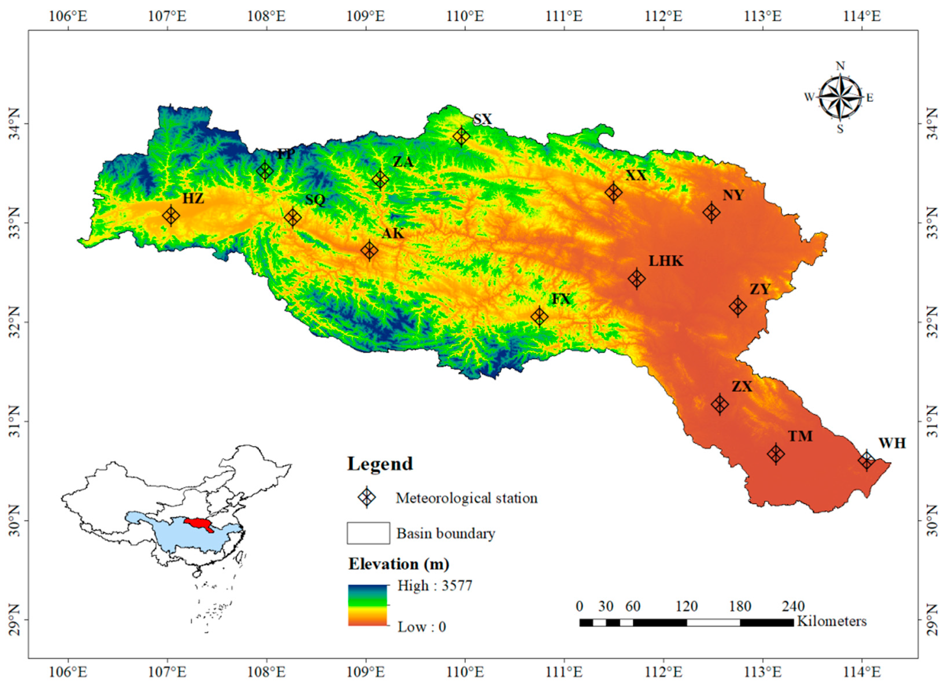
2.1. Study Region and Data Collection

The HRB, with an area of 1.59 × 10⁵ km², is located between 30°8′–34°11′ N and 106°12′–114°14′ E, and spans the provinces of Shanxi, Hubei, Henan, Sichuan, Gansu, and Chongqing (Figure 1). The primary stream of the HRB, with a length of 1577 km, is the largest tributary of the Yangtze River, China [19,20]. The west and central areas of the HRB are mountainous and semi-mountainous, whereas the east is a plain habitat with an elevation ranging from 0 to 3577 m (Figure 1). The basin is characterized by a subtropical monsoon climate with an average annual temperature ranging from 15 °C to 17 °C and annual average precipitation ranging from 700 to 1800 mm [19]. The precipitation distribution over a year is non-uniform, with precipitation between May and October accounting for 70–80% of the entire year. The runoff caused by precipitation from May to October accounts for approximately 75% of the annual total [19,20]. The HRB contains water sources for the Hanjiang to Weihe River Project and the South-to-North Water Diversion Project, which directly impact the water quality and quantity in China. The HRB is vulnerable to climate change and human activities [21]; thus, flood and drought disasters occur frequently in this region. It is essential to predict future precipitation changes in the HRB for disaster prevention and mitigation.

In this study, daily precipitation observations from 1970 to 2005 for 14 meteorological stations in the HRB (Figure 1 and

Table 1. HRB stations and their associated characteristics.

Station ID	Station Name	Abbreviation	Latitude (N)	Longitude (E)	Average Annual Precipitation 1970–2005 (mm)
57127	Hanzhong	HZ	33°04′	107°02′	853.52
57134	Foping	FP	33°31′	107°59′	910.92
57143	Shangxian	SX	33°52′	109°58′	683.58
57144	Zhenan	ZA	33°26′	109°09′	772.01
57156	Xixia	XX	33°18′	111°30′	851.51
57178	Nanyang	NY	33°06′	112°29′	777.54
57232	Shiquan	SQ	33°03′	108°16′	881.85
57245	Ankang	AK	32°43′	109°02′	826.32
57259	Fangxian	FX	32°03′	110°45′	831.05
57265	Laohekou	LHK	32°26′	111°44′	825.78
57279	Zaoyang	ZY	32°09′	112°45′	830.51
57378	Zhongxiang	ZX	31°10′	112°34′	964.83
57483	Tianmen	TM	30°40′	113°08′	1109.79
57494	Wuhan	WH	30°36′	114°03′	1259.42

) were obtained from the China Meteorological Administration (http://data.cma.cn/, accessed on 1 July 2021), which is responsible for monitoring, collecting, compiling, and releasing quality meteorological data in China. Data quality controls including missing value inspections and extreme value tests have been strictly implemented.

Twenty GCMs were selected for this study. Among these, 10 belong to CMIP5, for which precipitation simulation outputs were obtained from https://esgf-node.llnl.gov/search/cmip5/ (accessed on 1 July 2021), whereas 10 belong to CMIP6, for which precipitation simulation outputs were obtained from https://esgf-node.llnl.gov/search/cmip6/ (accessed on 1 July 2021). Monthly precipitation data from historical simulations of both model groups were used in this study. The variant labels of the CMIP6 and CMIP5 models are r1i1p1f1 and r1i1p1, respectively. The time period of the CMIP6 and CMIP5 precipitation data used in this study is 1970–2005 because of the data availability of the CMIP5 models.

Table 2. Studied GCMs from CMIP5 and CMIP6.

CMIP5		Modeling Center and Country	CMIP6
Model Name	Horizontal Resolution (Latitude × Longitude)		Model Name	Horizontal Resolution (Latitude × Longitude)
BCC-CSM1-1	2.8125° × 2.8125°	Beijing Climate Center, China	BCC-CSM2-MR	1.125° × 1.125°
BCC-CSM1-1-m	1.125° × 1.125°	Beijing Climate Center, China	BCC-ESM1	2.81° × 2.81°
FGOALS-g2	3° × 2.8°	Institute of Atmospheric Physics, Chinese Academy of Sciences, China	FGOALS-g3	2.3° × 2°
GISS-E2-H	2.5° × 2.5°	NASA Goddard Institute for Space Studies, USA.	GISS-E2-1-H	1.25° × 1.25°
CMCC-CM	0.75° × 0.75°	Centro Euro-Mediterraneo per I Cambiamenti Climatici, Italy	CMCC-CM2-SR5	1° × 1°
CMCC-CMS	1.875° × 1.875°	Centro Euro-Mediterraneo per I Cambiamenti Climatici, Italy	CMCC-CM2-HR4	0.25° × 0.25°
MIROC5	1.4° × 1.4°	Japan Agency for Marine-Earth Science and Technology, Japan	MIROC6	1.4° × 1.4°
IPSL-CM5A-LR	3.75° × 1.875°	Institut Pierre Simon Laplace, France	IPSL-CM6A-LR	1.26° × 2.5°
CanESM2	2.8125° × 2.8125°	Canadian Centre for Climate Modelling and Analysis, Canada	CanESM5	2.81° × 2.81°
MPI-ESM-LR	1.875° × 1.875°	Max Planck Institute for Meteorology, Germany	MPI-ESM1-2-LR	1.5° × 1.5°

lists the analyzed GCMs and their respective modeling centers, countries, and horizontal resolutions. Notably, although the GCM daily precipitation data can be obtained, we still selected GCM monthly precipitation data to evaluate and compare the precipitation simulation performances of the CMIP6 and CMIP5 models. Some previous studies indicated that GCM monthly outputs are more credible and accurate than the daily data [14,22,23,24]. Additionally, because of the coarse spatial resolution of GCM outputs, the inverse distance weighting method (IDW) was used to interpolate the GCM data at the four nearest neighboring grid points to the target meteorological station. Choosing GCM daily precipitation would have increased the difficulty of obtaining accurate wet spells. For example, when the target station was in a grid without daily rainfall, but the other grids received rainfall, wet spells would be increased artificially after interpolation. Because the MME has been demonstrated to exhibit superior performance compared to that of any individual model for analyzing CMIP historical simulations in the HRB [25,26], the CMIP5-MME and CMIP6-MME monthly precipitation values were used to compare the historical precipitation simulations of the CMIP5 and CMIP6 models with the observed data.

2.2. Methods

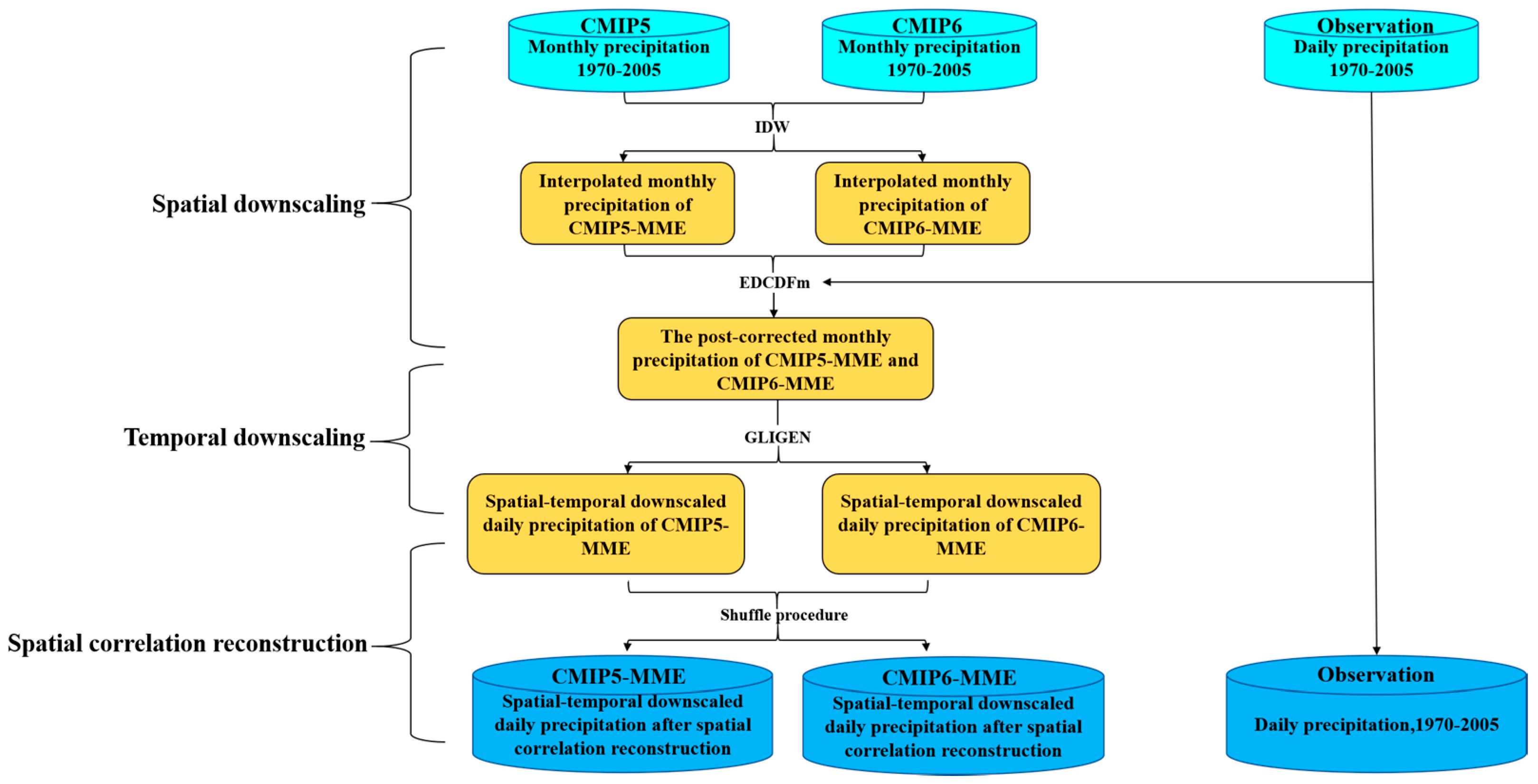
2.2.1. Downscaling Method

A multi-site statistical downscaling method introduced by Su et al. [12] was used to spatially and temporally downscale the GCM outputs. The method framework consists of three steps, as illustrated in Figure 2. The first step is spatial downscaling, which includes the IDW method and the equidistant cumulative distribution functions matching method (EDCDFm). The second step is temporal downscaling, in which the spatially downscaled monthly data are temporally downscaled into daily data using a single-site climate generator (CLIGEN). The final step re-creates the spatial correlation of the precipitation sequences for the meteorological stations based on the shuffle method [12].

(1) Spatial downscaling step:

In the spatial downscaling step, the IDW method and EDCDFm were applied. The IDW method interpolates the original large-scale GCM data at the four nearest neighboring grid points to the target meteorological station. The IDW method is expressed by Equations (1)–(3) [12,27]:

$$D={\cos }^{-1}\left(\cos {\alpha }_o\cos {\alpha }_s\left(\cos {\beta }_o\cos {\beta }_s+\sin {\beta }_o\sin {\beta }_s\right)+\sin {\alpha }_o\sin {\beta }_s\right)$$

(1)

$$W_j=\frac{1}{D_j}/{\displaystyle \sum }_{n=1}^4\frac{1}{D_j}$$

(2)

$$S_i={\displaystyle \sum }_{j=1}^4{W}_j\times S_j\left(t\right)$$

(3)

where D is the angular distance, α_o is the latitude of the target meteorological station, β_o is the longitude of the target meteorological station, α_s is the grid point latitude, and β_s is the grid point longitude. W_j is the weight of four GCM grid points that are closest to the target meteorological station. S_j is the value of the climatic variable of the GCM grid points, and S_i represents the mean weighted sum of the climatic variable for timescale t. Using the above equations, interpolated GCM-generated precipitation data for CMIP5 and CMIP6 were obtained. Finally, the CMIP5-MME and CMIP6-MME values were obtained through calculations.

The deviation in the interpolated data of CMIP5-MME and CMIP6-MME must be corrected; this was performed using EDCDFm. EDCDFm modifies the shape of the theoretical probability distribution function of the simulated precipitation data based on the shape of the theoretical probability distribution function of the observed precipitation data. Additional details regarding EDCDFm have been described by Su et al., Li et al., and Chen et al. [12,28,29]. EDCDFm can be written mathematically as Equation (4) [12].

$${\tilde{x}}_{m-f,cor}=x_{m-f}+F_{o-c}^{-1}\left(F_{m-f}\left(x_{m-f}\right)\right)-F_{m-c}^{-1}\left(F_{m-f}\left(x_{m-f}\right)\right)$$

(4)

where ${\tilde{x}}_{m-f,cor}$ is the post-corrected GCM monthly data, x_m−f is the pre-corrected GCM monthly data, $F_{o-c}^{-1}$($F_{m-c}^{-1}$) is the cumulative distribution inverse function (CDF) of the observed monthly data, and F_m−f is the CDF of the GCM monthly data. Finally, the monthly precipitation of the CMIP5-MME and CMIP6-MME were spatially downscaled using the IDW method and EDCDFm, respectively.

(2) Temporal downscaling step:

In the temporal downscaling step, the CLIGEN model was used to downscale the precipitation data generated by the GCMs from the monthly scale to the daily scale. The CLIGEN is a stochastic weather generator that is often used to generate daily weather series from monthly GCM projections for climate change impact studies [30,31]. There are five input parameters, which are determined by the observed daily precipitation, and are required for CLIGEN to downscale GCM-generated monthly precipitation to daily precipitation: P_w, average daily precipitation on wet days; S_d, standard deviation of wet day precipitation; S_kew, coefficient of skewness of wet day precipitation; P_W|W, probability of a wet day following a wet day; and P_W|D, probability of a wet day following a dry day. Among these, the S_kew of the GCM output was assumed to be the same as that of the observed data. To determine the other four parameter values, the following procedure was performed as described by Su et al. [12]:

Observed daily precipitation data for 1970–2005 for each month and site were first used to compute the mean (R_m), variance, and the five CLIGEN parameters. Second, a linear relationship between R_m and P_W|D for each month and all sites was assumed to estimate the future wet-following-dry transition probability. We assumed that the probability of the occurrence of a wet day (R_d) was proportional to P_W|D. The mathematical expressions can be expressed as Equations (5) and (6).

$$P_{W|D}=a+b\times R_m$$

(5)

$$R_d=\left(R_m\left(1-P_{W|W}+P_{W|D}\right)\right)/\left(N_d\times P_{W|D}\right)$$

(6)

It follows that

$$P_{W|D}^{\prime }=\alpha \times R_d$$

(7)

$$P_{W|W}^{\prime }=1-\alpha +P_{W|D}^{\prime }$$

(8)

where a and b are constants, N_d is the number of days in the month, and $P_{W|W}^{\prime }$ and $P_{W|D}^{\prime }$ are the new $P_{W|W}$ and $P_{W|D}$, respectively.

Finally, when changes in $P_{W|W}$ and $P_{W|D}$ were small, the standard deviation for climate projections based on the GCM data was calculated as shown in Equation (9).

$$S_d=S_{do}\sqrt{\frac{V}{V_o}}$$

(9)

where S_d and S_do are the standard deviations of the daily precipitation on wet days for the GCM output and observed data, respectively, and V and V_o are the variances of the monthly precipitation for the GCM output and the observed data, respectively.

Using these methods, the parameters for each station were adjusted separately for the GCM-generated historical precipitation data. These adjusted parameters were then inputted into CLIGEN, and the daily series precipitation data of each station were generated for CMIP5-MME and CMIP6-MME during the period from 1970 to 2005.

(3) Spatial correlation reconstruction:

The CLIGEN downscaling method can only produce climate change scenarios at a single site or independently at multiple sites [14]. However, the spatial correlation between meteorological stations should be considered to maintain physical coherence. The negligence of inter-site dependence in the downscaled meteorological fields can lead to misrepresentation of the hydrological response variables in subsequent hydrological impact studies [24]. Therefore, after temporal downscaling using the CLIGEN model, the spatial correlation between stations in the HRB must be reconstructed. In this study, the shuffle procedure provided by Su et al. [12] was used to rebuild the spatial correlations. The details of this method have been described by Su et al. [12].

2.2.2. Assessment of Downscaling Methodology

Assessment of the downscaling method used to downscale the CMIP5-MME and CMIP6-MME contained the following aspects. (1) To evaluate the performance of the deviation correction in spatial downscaling for the CMIP5-MME and CMIP6-MME, the mean and standard deviation were used. The calculation methods are expressed as Equations (10) and (11). (2) To evaluate the performance of the CLIGEN model in temporal downscaling for the CMIP5-MME and CMIP6-MME, a quantile-quantile (QQ) plot of the daily precipitation amount was used. (3) To assess the performance of the shuffle procedure in spatial correlation reconstruction, the emphasis was placed on its capability to restore the observed inter-station dependencies. The inter-station spatial correlation coefficient of the relationship between precipitation values before and after spatial correlation reconstruction (using the shuffle procedure) for CMIP5-MME and CMIP6-MME was considered in this study.

$$M={\displaystyle \sum }_{i=1}^n\frac{x_i}{n}$$

(10)

$$SD=\sqrt{\frac{{{\displaystyle \sum }}_{i=1}^n{\left(x_i-M\right)}^2}{n-1}}$$

(11)

where x_i is the CMIP5-MME, CMIP6-MME, or observed monthly precipitation data; and n is the total number of months.

2.2.3. Comparison Indices and Methods

The performance evaluation of the downscaled CMIP5-MME and CMIP6-MME for precipitation simulation emphasize the capability to reproduce spatial patterns, temporal patterns, and seasonal variations. For the capability to describe a spatial pattern, the spatial distribution map of daily average precipitation and biases between the GCMs’ downscaled data and observational data were used; for the capability to describe a temporal pattern, box plots of monthly average precipitation and biases between the GCMs’ downscaled data and observational data were used; for the capability to describe seasonal variations, the spatial distribution map of seasonal precipitation and biases between the GCMs’ downscaled data and the observational data of each station in the winter, spring, summer, and autumn were used.

3. Results

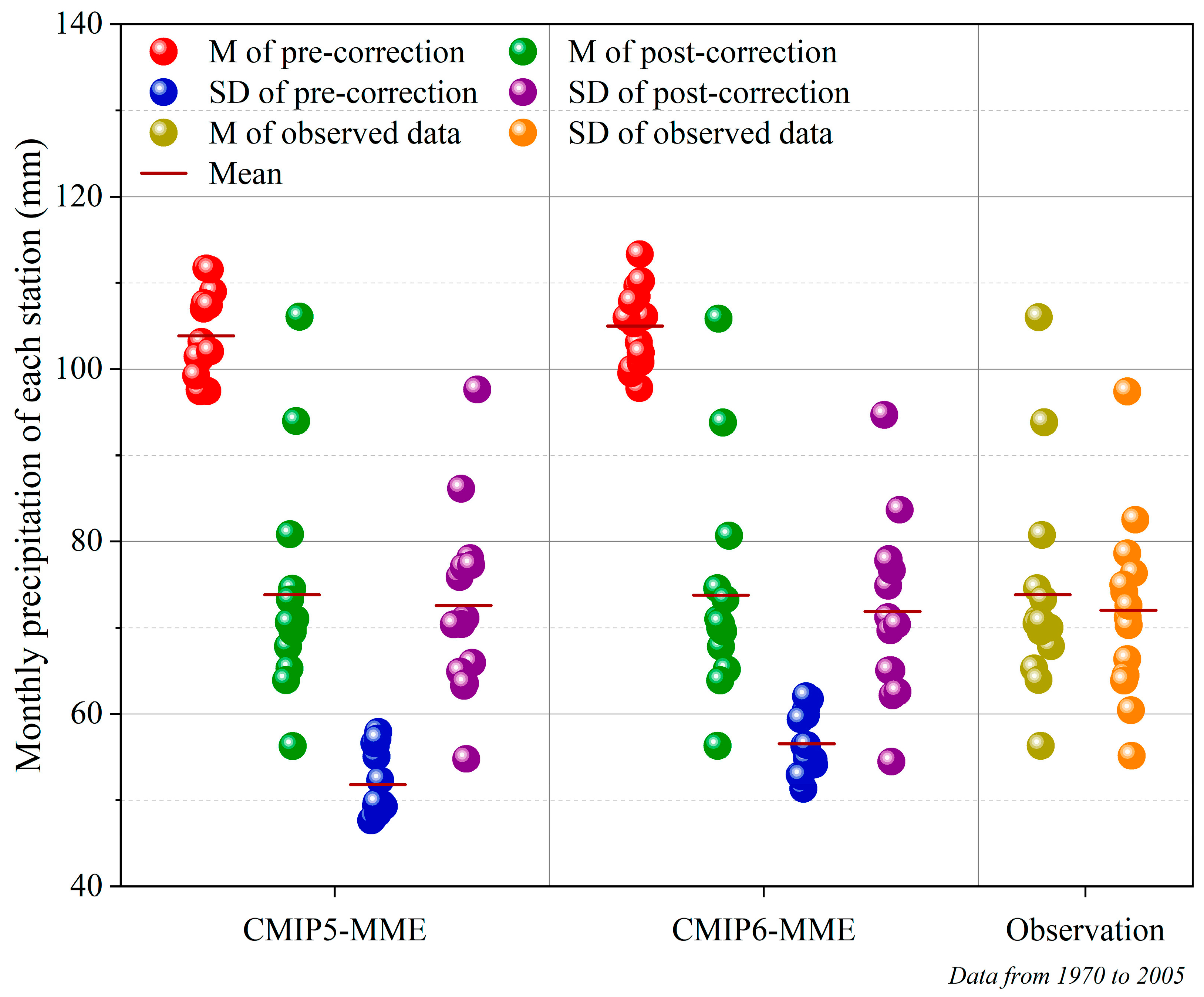
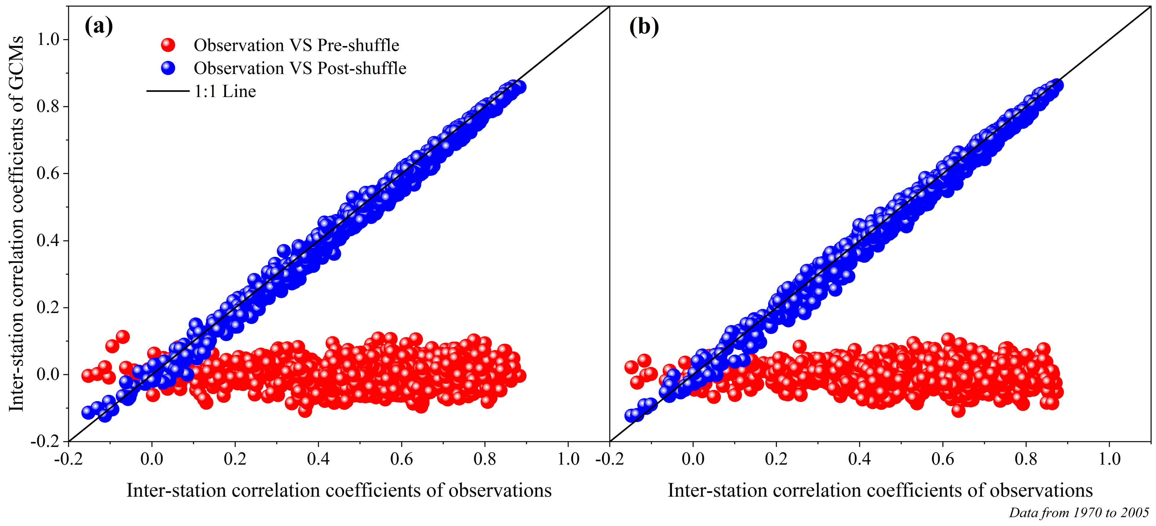
3.1. Assessment of Downscaling Results

After spatial downscaling, the deviation correction results of the CMIP5-MME and CMIP6-MME monthly precipitation data were verified. The mean and standard deviation of monthly precipitation before and after the deviation correction of the CMIP5-MME and CMIP6-MME were compared with the observed monthly precipitation for each station, as shown in Figure 3. Before deviation correction, the mean values of the monthly precipitation of CMIP5-MME and CMIP6-MME were larger than those of the observed data for all stations, and the standard deviations were smaller. After deviation correction, the mean and standard deviation values were nearly equal to those of the observed data for each station. The results demonstrate that the performances of the CMIP5-MME and CMIP6-MME were significantly improved after deviation correction, indicating that the EDCDFm is suitable.

After temporal downscaling, the downscaled daily values for 14 stations in the HRB were evaluated. The QQ plots of observation versus GCM daily precipitation data for the CMIP5-MME and CMIP6-MME are shown in Figure 4, where the quantiles varied from 0.5 to 99.9 when the stations were aggregated. The station scatter plot points followed a 1:1 line, indicating that the downscaled daily precipitation of the CMIP5-MME and CMIP6-MME fit the observed data well, and the two distributions were similar. When precipitation was low, the downscaled daily precipitation of the CMIP5-MME and CMIP6-MME correlated well with the observed data. However, as precipitation increased, the scatter plot points gradually began to deviate from the 1:1 line, indicating that the CLIGEN model has a weak ability to simulate extreme precipitation, which is consistent with the findings of Su et al. [12].

After the shuffle procedure, the inter-station spatial correlation coefficients of the CMIP5-MME and CMIP6-MME were compared with the observed data, as shown in Figure 5. Before shuffling, the inter-station correlation coefficients of the CMIP5-MME and CMIP6-MME were between −0.2 and 0.2, and the scatter plot points were far from the 1:1 line (Figure 5), indicating that the spatial correlations between stations in the HRB were inconsistent with the observed data. After shuffling, the inter-station correlation coefficients of the CMIP5-MME and CMIP6-MME were between −0.2 and 0.85, and the scatter plot points were distributed around the 1:1 line (Figure 5), indicating that the inter-station correlation was equal or close to that of the observed data. The results indicate that the shuffle procedure effectively restores the spatial correlation structures of the CMIP5-MME and CMIP6-MME downscaled daily precipitation data compared to those of the observed data.

The results demonstrate that the downscaling method used in this study, proposed by Su et al. [12], can be applied to address the problem of the coarse temporal and spatial resolutions of the CMIP5-MME and CMIP6-MME for the HRB. The temporal and spatial downscaling results of the GCM data can be used to evaluate and compare the precipitation simulations of the CMIP5 and CMIP6 projections in the HRB.

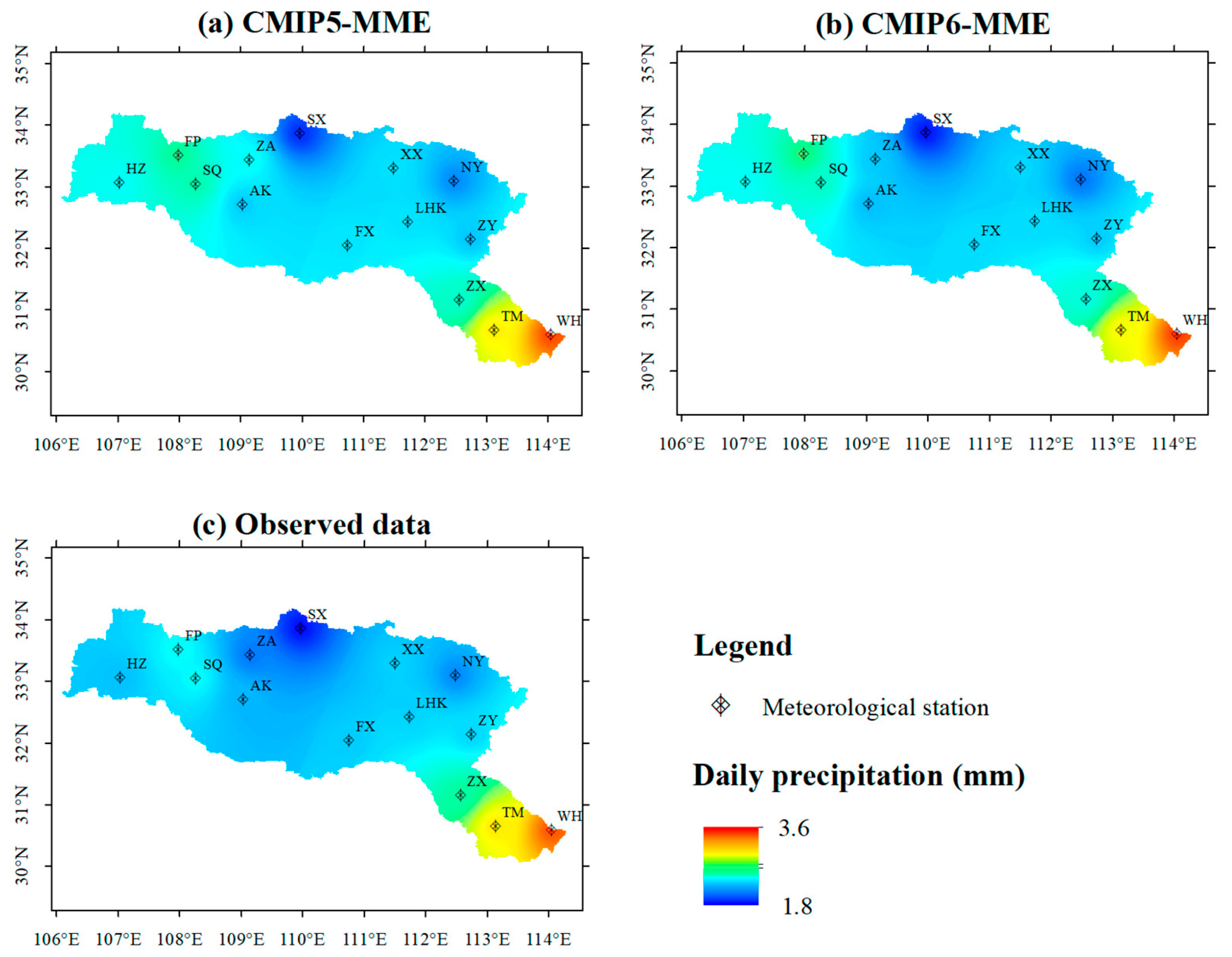
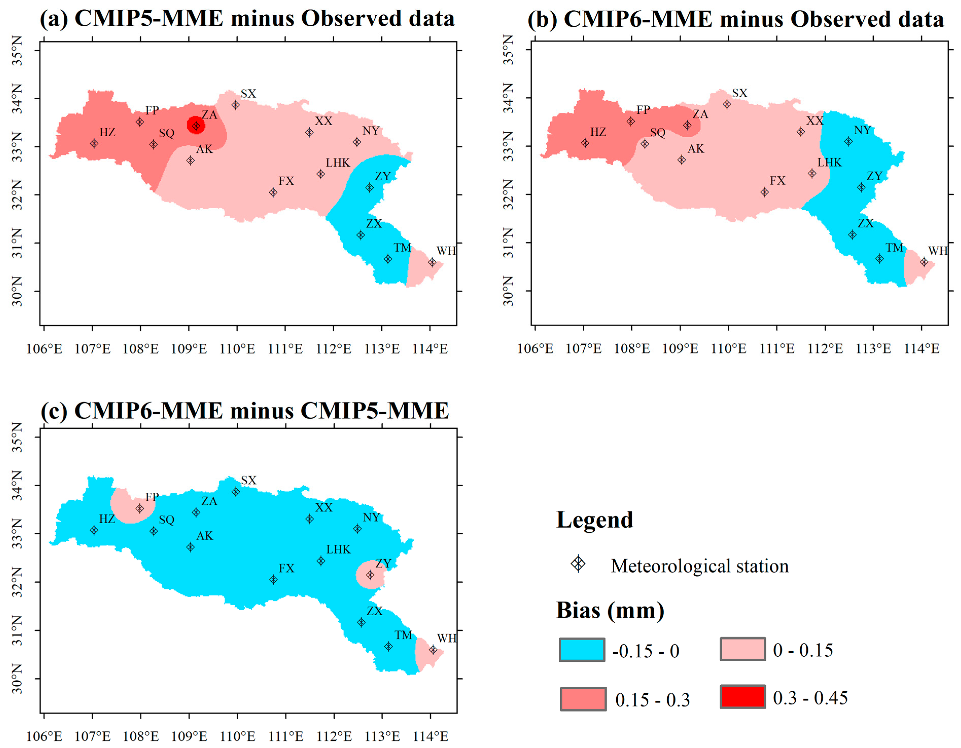
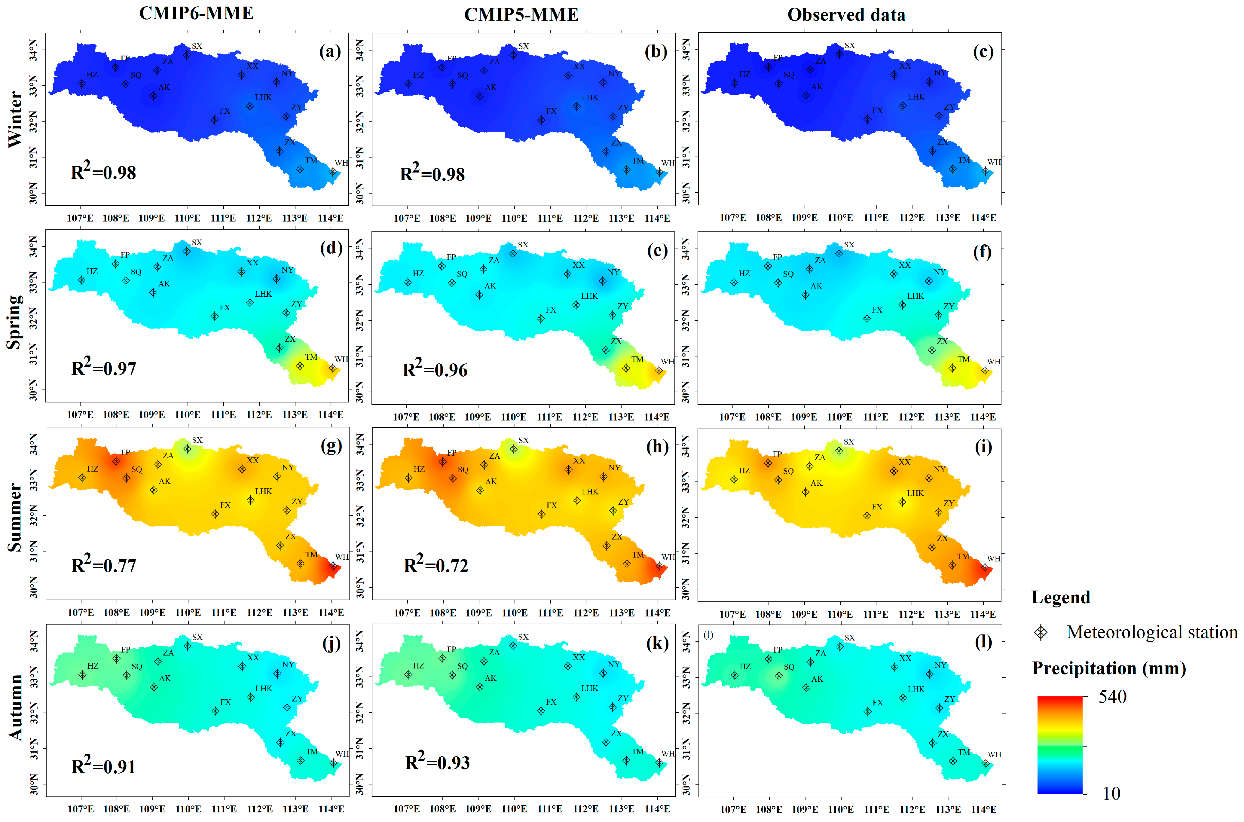
3.2. Spatial Performance Comparison of CMIP5-MME and CMIP6-MME Downscaled Precipitation

Using the observed and downscaled GCM precipitation of the 14 meteorological stations, the IDW method was leveraged to obtain spatial distribution maps of the mean daily precipitation, as illustrated in Figure 6. The maps compare the precipitation pattern over the HRB from 1970 to 2005 depicted by the CMIP5-MME and CMIP6-MME downscaled data with that of the observed data. The precipitation spatial pattern of the CMIP5-MME (Figure 6a) and CMIP6-MME downscaled data (Figure 6b) reflect that of the observed precipitation (Figure 6c) in the HRB. The precipitation distributions of the CMIP5-MME downscaled data, CMIP6-MME downscaled data, and observed data decrease from southeast to northwest over the HRB, except for areas monitored by the FP, HZ, and SQ stations. The maximum precipitation was observed at the WH station; the CMIP5-MME downscaled data, CMIP6-MME downscaled data and observed data values were 3.48, 3.51, and 3.46 mm/d, respectively. The minimum precipitation amount was observed at the SX station; the CMIP5-MME downscaled data, CMIP6-MME downscaled data, and observed data values were 1.88, 1.84, and 1.83 mm/d, respectively.

Figure 7 illustrates the spatial patterns of the daily precipitation biases between the CMIP5-MME downscaled data and observed data, and the CMIP6-MME downscaled data and observed data in 1970–2005 over the HRB. The daily precipitation biases of the CMIP5-MME and CMIP6-MME downscaled data were similar, with excess precipitation in the west and central areas and deficient precipitation in the eastern HRB, except for the area monitored by the WH station. The results indicate that the downscaled CMIP5-MME and the CMIP6-MME precipitation simulations slightly overestimated precipitation in the western and central areas of the HRB and slightly underestimated precipitation in the eastern area of the HRB, except for at the WH station. The downscaled CMIP6-MME bias values of 10 stations accounted for 72% of all stations and are smaller than those of the downscaled CMIP5-MME. The highest precipitation bias value between the CMIP5-MME downscaled data and the observed data was 0.34 mm/d, occurring at the ZA station; the highest precipitation bias value between the CMIP6-MME downscaled data and observed data was 0.28 mm/d, occurring at the FP station. These results illustrate that the precipitation simulation biases of the CMIP6 models were smaller than those of the CMIP5 models. In addition, the bias between the CMIP5-MME and CMIP6-MME downscaled data indicates that the downscaled CMIP6-MME reduced the precipitation bias in the western and central areas of the HRB.

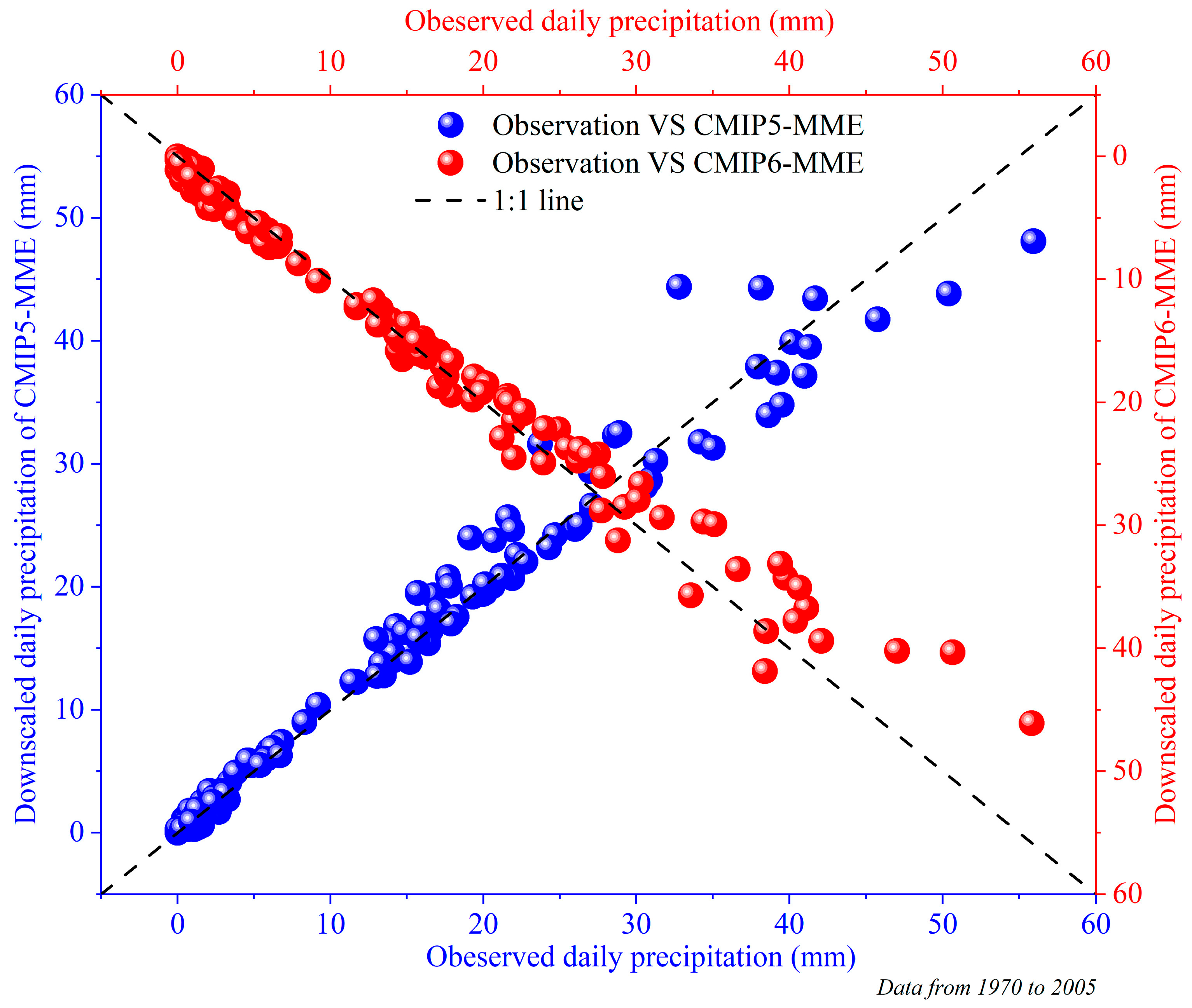
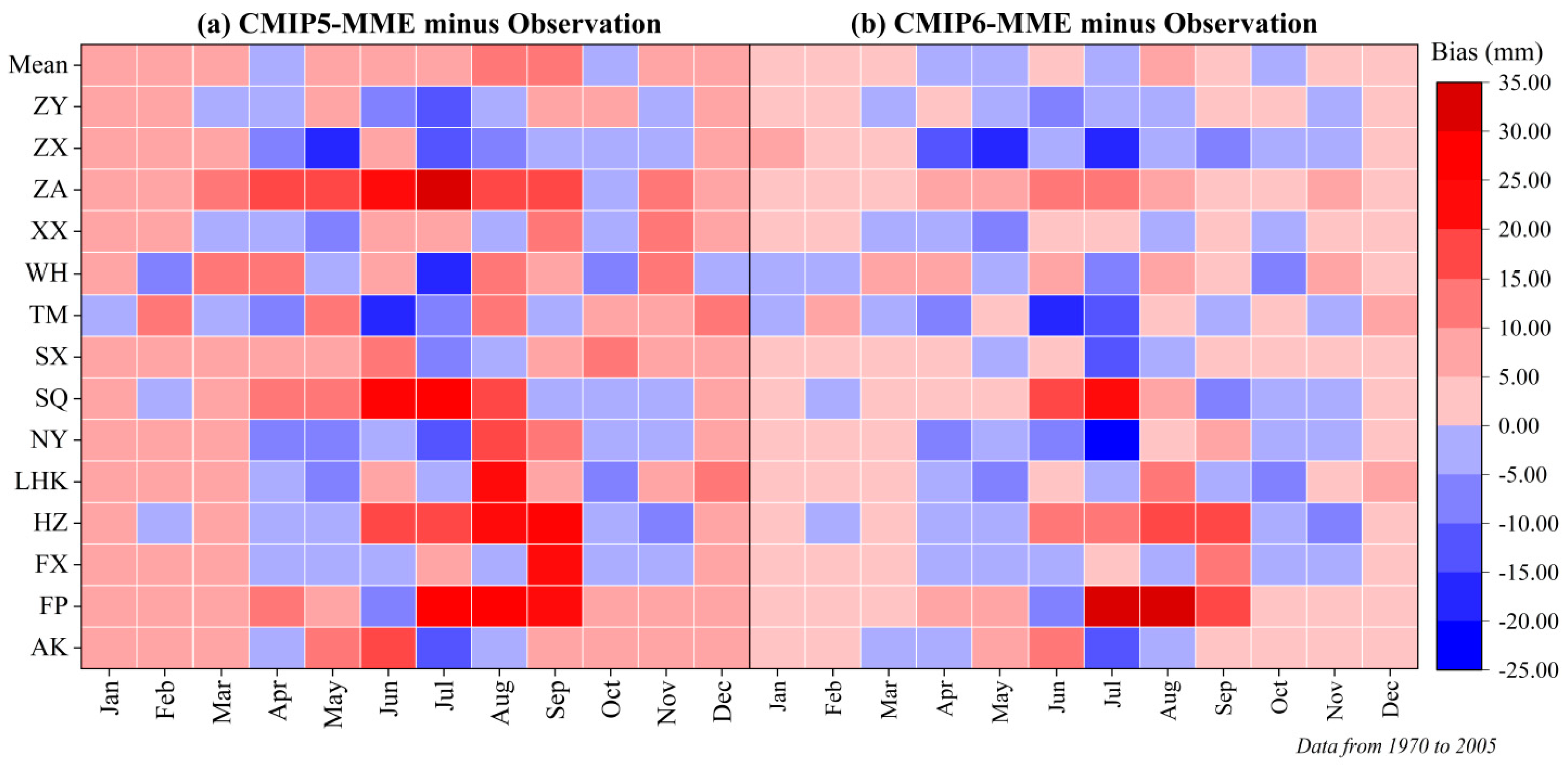
3.3. Temporal Performance Comparison of CMIP5-MME and CMIP6-MME Downscaled Precipitation

According to the observed and GCM downscaled daily precipitation from the 14 meteorological stations, the average monthly precipitation for each month from 1970 to 2005 was calculated and compared, as illustrated in Figure 8, through box and scatter plots of the CMIP5-MME downscaled data, CMIP6-MME downscaled data, and observed data. The downscaled monthly precipitation distributions of the CMIP5-MME and CMIP6-MME data are typically consistent with those of the observed data. The downscaled monthly precipitation of the CMIP5-MME data was slightly greater than that of the observed data in January, February, March, May, June, July, August, September, November, and December, whereas that of the CMIP6-MME was greater than that of the observed data in January, February, March, June, August, September, and December. The mean monthly precipitation ranges of the CMIP5-MME downscaled data, the CMIP6-MME downscaled data, and the observed data from 1970 to 2005 were 15.27–162.86, 15.25–160.73, and 12.63–161.05 mm, respectively.

Figure 9 displays the biases of the average monthly precipitation between the GCMs’ downscaled data and observed data for each station and month. Overall, the biases between the GCMs’ downscaled data and the observed data were small, except for the precipitation of the CMIP5-MME in June, July, August, and September and that of the CMIP6-MME in July and August, when the bias exceeded 20 mm. These months include the rainy days of the HRB. These results indicate that the downscaled CMIP6 and CMIP5 GCMs poorly simulate heavy rainfall. Figure 9 also displays the mean monthly precipitation in each month. The maximum bias of the monthly precipitation between the CMIP5-MME downscaled data and observed data was 6.84 mm, and that between the CMIP6-MME downscaled data and observed data was 5.74 mm in August. The mean biases in most months from January to December between the CMIP6-MME downscaled data and observed data were smaller than those between the CMIP5-MME downscaled data and observed data. The results indicate that the ability of the downscaled CMIP6-MME in simulating temporal performance is superior to that of the downscaled CMIP5-MME.

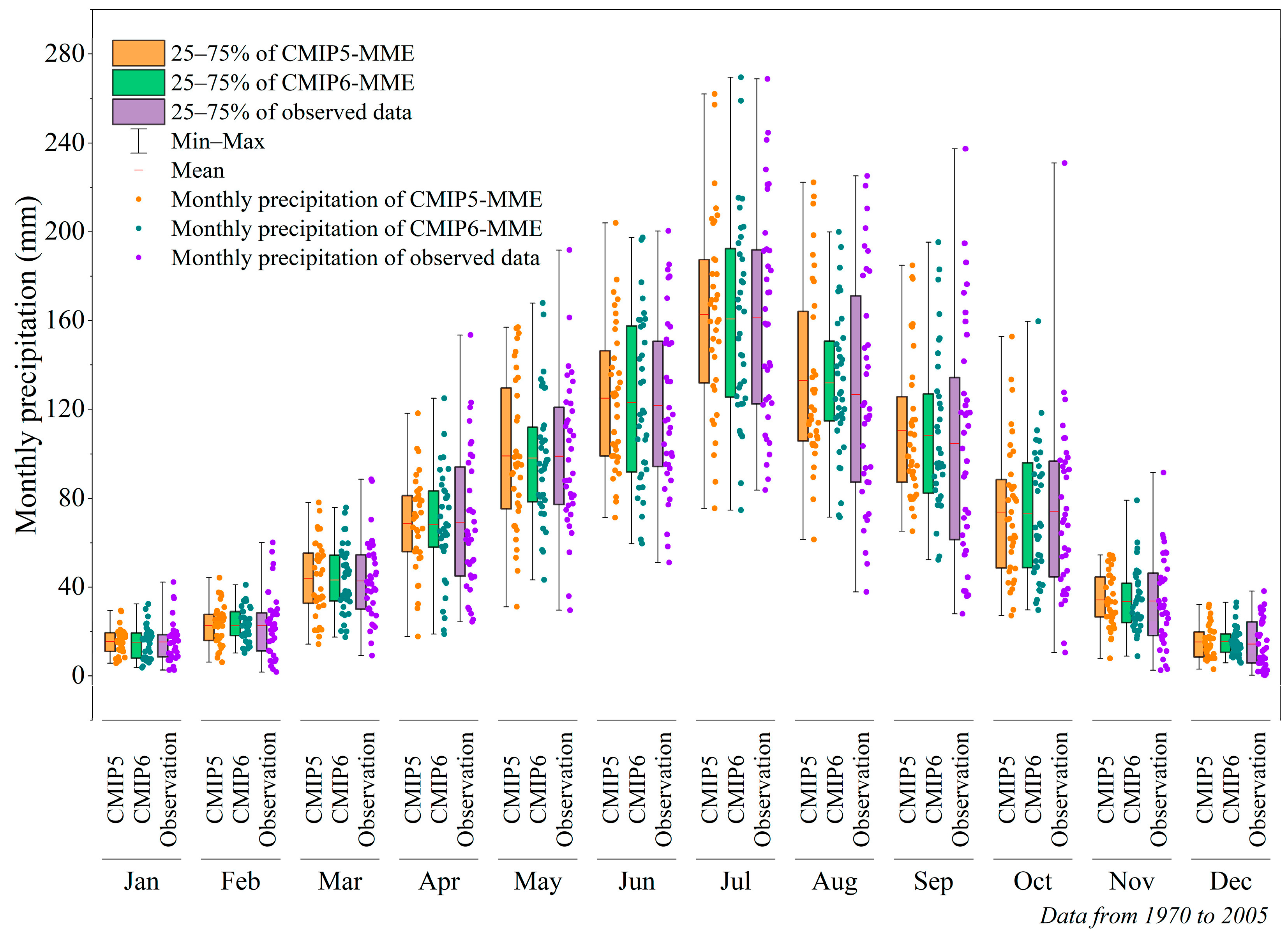
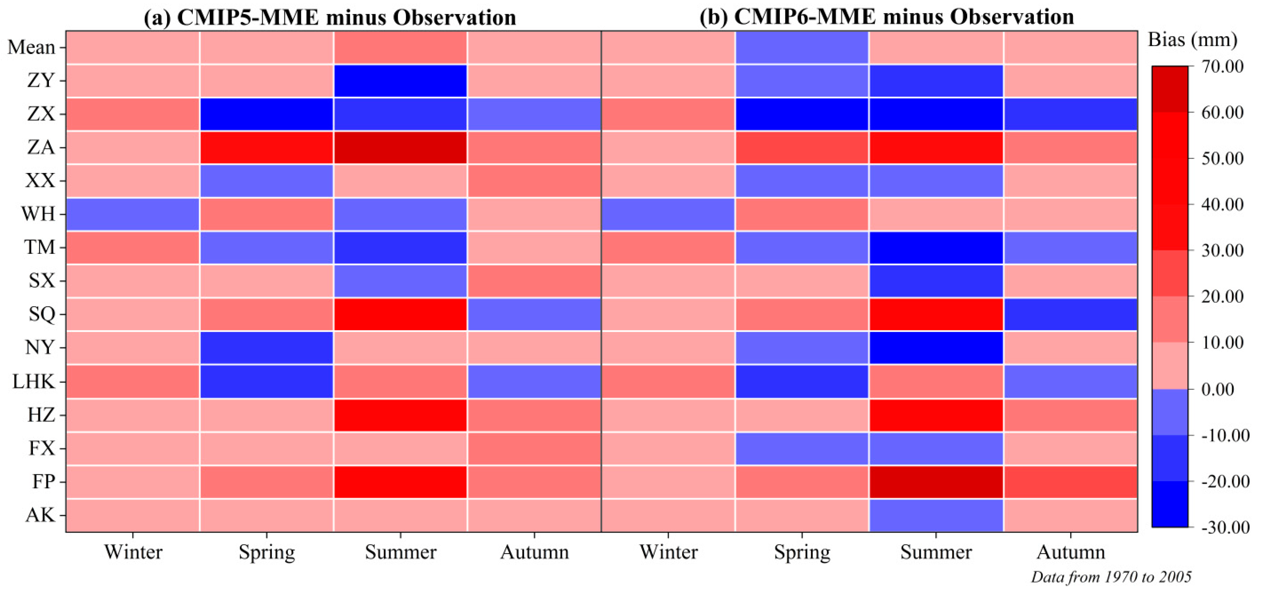
3.4. Seasonal Variation Comparison of CMIP5-MME and CMIP6-MME Downscaled Precipitation

Using the observed and downscaled GCM daily precipitation from the 14 meteorological stations, the IDW method was used to obtain the spatial distribution map of precipitation in winter, spring, summer, and autumn, as illustrated in Figure 10. The downscaled precipitation spatial patterns of CMIP6-MME and CMIP5-MME were consistent with those of the observed data across seasons. In winter (Figure 10a–c), the precipitation decreases from southeast to northwest, and the maximum precipitation of the observed data, the CMIP6-MME downscaled data, and the CMIP5-MME downscaled data occurred at the WH station (131.45, 127.41, and 125.51 mm, respectively). In spring (Figure 10d–f), the precipitation in the southeast area was the greatest, and the maximum precipitation of the observed data, the CMIP6-MME downscaled data, and the CMIP5-MME downscaled data occurred at the WH station (392.58, 403.63, and 408.96 mm, respectively). In summer (Figure 10g–i), the southeast, northwest, and northeast areas exhibited greater precipitation compared with that of the central area, and the maximum precipitation of the observed data, the CMIP6-MME downscaled data, and the CMIP5-MME downscaled data occurred at the WH station (524.49, 532.28, and 518.86 mm, respectively). In autumn (Figure 10j–l), the precipitation in the northwest area was greatest, and the maximum precipitation of the observed data, the CMIP6-MME downscaled data, and the CMIP5-MME downscaled data occurred at the SQ, FP, and HZ stations (261.25, 264.93, and 263.03 mm, respectively), respectively. Figure 10 also displays the linear determination coefficients (R²) between the downscaled GCMs’ precipitation and observed data in different seasons. The R² values in winter, spring, and autumn are above 0.9 not only for CMIP6-MME but also for CMIP5-MME. However, the R² of CMIP6-MME and CMIP5-MME in summer were only 0.77 and 0.72, respectively, indicating that the downscaled CMIP5 and CMIP6 GCMs poorly simulate precipitation during the rainy season.

Figure 11 displays the average seasonal precipitation biases between the GCMs’ downscaled data and the observed data for each station. In winter, biases between the CMIP6-MME downscaled data and the observed data were smaller than those between the CMIP5-MME downscaled data and the observed data for 79% of stations. In spring and autumn, the downscaled CMIP6-MME exhibited a lower bias than the downscaled CMIP5-MME for 57% of stations. However, the downscaled CMIP5-MME outperformed the downscaled CMIP6-MME for 64% of stations in summer. There were substantial differences in the bias values. In winter, the maximum biases of the CMIP5-MME and CMIP6-MME downscaled data occurred at the LHK station (12.6 and 12.18 mm, respectively). In spring, the maximum bias of the CMIP5-MME downscaled data occurred at the ZA station (34.85 mm), and that of the CMIP6-MME downscaled data occurred at the ZX station (−27.34 mm). In summer, the maximum CMIP5-MME downscaled data bias occurred at the ZA station (62.69 mm), and that of the CMIP6-MME downscaled data occurred at the FP station (60.35 mm). In autumn, the maximum biases of the CMIP5-MME and CMIP6-MME downscaled data occurred at the FP station (18.32 and 20.74 mm, respectively). In winter, the mean biases of the CMIP5-MME and CMIP6-MME downscaled data were 6.78 and 6.69 mm, respectively. In spring, the mean biases of the CMIP5-MME and CMIP6-MME downscaled data were 2.21 and −0.02 mm, respectively. In summer, the mean biases of the CMIP5-MME and CMIP6-MME downscaled data were 12.21 and 7.01 mm, respectively. In autumn, the mean biases of the CMIP5-MME and CMIP6-MME downscaled data were 6.48 and 2.96 mm, respectively. Based on these results, the seasonal precipitation simulation capabilities of the downscaled CMIP6-MME were stronger for most stations compared to those of the downscaled CMIP5-MME in winter, spring, and autumn, and were weaker in summer. The bias value results indicate that the seasonal precipitation simulation performances of the downscaled CMIP6 models were improved compared with those of the downscaled CMIP5 models.

4. Discussion

In this study, temporally and spatially downscaled precipitation data from 20 GCMs from CMIP6 and CMIP5 projections were used to evaluate the precipitation simulation performance for HRB, China. Comparison of the results with observed data during the period of 1970–2005, showed that both the downscaled CMIP5-MME and CMIP6-MME captured the spatial pattern, temporal pattern, and seasonal variation precipitation characteristics in the HRB. However, certain biases remain for the downscaled GCM precipitation simulations. The precipitation simulation biases of CMIP6-MME downscaled data were lower than those of CMIP5-MME downscaled data, indicating that the downscaled CMIP6-MME reduced the precipitation bias. These findings are consistent with those of some previous studies. Gusain et al. [8] assessed CMIP5 and CMIP6 GCM precipitation simulations for indicative characteristics that represent the complex dynamics of Indian summer monsoon rainfall and found significant improvement in CMIP6 models in capturing the spatiotemporal pattern of monsoon rainfall over India, particularly in the Western Ghats and the northeast foothills of the Himalayas. Rivera and Arnould [17] evaluated the ability of CMIP6 precipitation simulation historical runs to capture the complex spatial and temporal patterns observed over southwestern South America, with the results demonstrating that the primary features of regional precipitation were adequately captured by most CMIP6 models. Srivastava et al. [32] found that the multi-model medians of CMIP6 and CMIP5 exhibit similar biases in climatology and variability, but those of the CMIP6 tend to be smaller.

Our results illustrate that the precipitation simulation capabilities of the downscaled CMIP6-MME at most stations were stronger than those of the downscaled CMIP5-MME in winter, spring, and autumn, whereas they were weaker in summer. However, Zamani et al. [33] found that CMIP6 models exhibited superior performance compared to that of the CMIP5 models at most stations in winter, spring, and summer and weaker performance in autumn. These differing results may be related to differences in the location and climate type between the two study regions. Zamani et al. [33] selected an arid region in the west of Asia between the latitudes 24° N and 40° N and longitudes 44° E and 64° E, which exhibits a tropical desert climate. The seasons of a tropical desert climate are dry and less rainy. The study region of our research is the HRB, which is in the east of Asia and belongs to a subtropical monsoon zone. The subtropical monsoon climate is mild and humid, and precipitation is abundant.

According to the spatial distribution comparisons, the results indicate that the CMIP5-MME and CMIP6-MME downscaled simulations slightly overestimated precipitation in the western and central HRB and slightly underestimated precipitation in the eastern HRB. These results may be related to elevation and urbanization. The central and western HRB belong to the upstream and midstream of the basin, which contain mountainous and semi-mountainous areas (Figure 1), respectively, and the elevation is typically greater than 3000 m. Some studies [34,35] reported that precipitation typically increases with elevation but after reaching a certain height, precipitation begins to decrease. Because air rises because of the uplift of the terrain, it cools and condenses to form precipitation. However, as the elevation increases, the moisture content in the air decreases, and the precipitation decreases rather than increases. Other studies showed that precipitation increases with elevation, with inverse cases sometimes occurring locally because of the topographic and meteorological features of the area [36]. This may have caused the GCMs to overestimate the precipitation in the central and western HRB. The eastern HRB is downstream, which belongs to the plain area, and most cities are in this region. Because of urbanization, many cities experience the rain island effect, with increased precipitation in cities. Sahoo et al. [37] discussed the impact of urbanization on rainfall processes and mechanisms using the weather research and forecasting model, and the simulation results illustrated that the current urbanization scenario exhibits a significant increase in rainfall by over 100–200%. Kishtawal et al. [38] assessed the impacts of urbanization on heavy rainfall climatology and concluded that an increasing trend for heavy rainfall event frequency is more likely for regions where the urbanization rate is greater. Therefore, the urbanization rain island effect may have led to the underestimation of the GCM-simulated precipitation in the eastern HRB.

Our results indicate that the precipitation simulation abilities of the downscaled CMIP5-MME and CMIP6-MME are poor during rainy months and seasons (rainy days) in the study region. This result may be related to the downscaling method. As described in Section 3.1, the CLIGEN model showed a weak ability to simulate extreme precipitation, which is supported by many scholars [12,31,39]. However, this result may also be related to the poor simulation performance of GCM on rainy days over the HRB. Because of the availability of observational data, the daily precipitation observations from 1970 to 2005 for 14 meteorological stations collected in the HRB were employed to verify the GCMs’ simulations in this study. Based on the limitations of the observational station data, a multi-site downscaling method was required in this study. Although the observational data used in this study were able to represent the spatiotemporal variability of precipitation, precipitation accuracy could have been assessed against a gridded precipitation dataset in addition to meteorological stations. There are dozens of gridded precipitation datasets and reanalysis data available in previous studies [40,41,42]. In the future, a gridded precipitation dataset must be applied to verify the GCMs’ simulation outputs, and another bias correction method, such as the quantile mapping method, will be used. Furthermore, extreme climate indices will be selected to explore and compare the model performance of the CMIP6 and CMIP5 in simulating precipitation extremes over the HRB in the future.

A multi-site statistical downscaling method was used to spatially and temporally downscale the GCM outputs. There are errors in the P_W|W and skewness coefficient in the CLIGEN model, which depends on the first-order two-state Markov chain [12]. Although this Markov chain has been demonstrated to have sufficient applicability in simulating the probability of precipitation transitions [30,43], a high-order multi-state Markov chain must be used in future studies because of the lack of physical mechanisms [12]. Compared with the statistical downscaling method, the dynamic downscaling method exhibits a clear physical mechanism that can accurately simulate the regional climate variable features and characterize the precipitation spatial pattern and convection processes of a catchment [44,45]. Therefore, a dynamic downscaling method with a higher spatial resolution should be considered in future studies. In addition, to compare the precipitation simulations of CMIP5 and CMIP6 to the observed precipitation data, only 10 GCMs from CMIP5 and 10 GCMs from CMIP6 were used in this study because of data limitations. There are substantial uncertainties in the precipitation simulation trends for the CMIP5 and CMIP6 GCMs. Additional evaluations of more GCMs are needed to comprehensively understand the precipitation simulations in CMIP5 and CMIP6.

5. Conclusions

GCMs can provide essential meteorological data for simulating and assessing the impact of climate change on regional hydrology. Selecting appropriate GCM output data is the basis for accurate hydrology simulation prediction. In addition, because of the coarse temporal and spatial resolutions of the GCMs, an effective downscaling method is often required to study regional climatic conditions and hydrological processes. In this study, a multi-site statistical downscaling method was applied to spatially and temporally downscale the precipitation simulations of CMIP5-MME and CMIP6-MME.

The multi-site statistical downscaling method contains a spatial downscaling step that utilizes the IDW and EDCDFm methods, a temporal downscaling step using the CLIGEN model, and a spatial correlation reconstruction step suing a shuffle procedure method. The CMIP5-MME and CMIP6-MME precipitation mean and standard deviation values were used to evaluate the spatial downscaling step, QQ plots of the daily precipitation were used to evaluate the temporal downscaling step, and inter-station spatial correlation coefficients of the CMIP5-MME and CMIP6-MME were used to evaluate the spatial correlation reconstruction step. The results of all downscaling steps passed accuracy evaluation. The temporal and spatial downscaling results of the GCM data can be used to evaluate and compare the CMIP5 and CMIP6 precipitation simulations for the HRB.

A spatial distribution map, biases between the GCMs’ downscaled precipitation data and the observed data, and box plots were used to evaluate the performances of the downscaled CMIP5-MME and CMIP6-MME precipitation simulations compared with the observed data in the HRB from 1970 to 2005. The results illustrate that (1) the downscaled CMIP5-MME and CMIP6-MME can capture the spatial pattern, temporal pattern, and seasonal variations in the HRB but overestimate precipitation in the western and central HRB and underestimate precipitation in the eastern HRB; (2) the precipitation simulation biases of the downscaled CMIP6-MME are smaller than those of the downscaled CMIP5-MME, demonstrating improvement for CMIP6-MME in reducing precipitation bias; (3) the precipitation simulation capabilities of the downscaled CMIP6-MME in most stations are stronger than those of the downscaled CMIP5-MME in winter, spring, and autumn but are weaker in summer; and (4) the abilities of both the downscaled CMIP5-MME and CMIP6-MME in simulating precipitation on rainy days are poor, which may be related to the CLIGEN model. Our study provides a reference for data reliability to drive the hydrological model simulation and the prediction of future hydrologic cycles. Future studies should focus on the comparison of additional GCM precipitation simulation from CMIP5 and CMIP6 and the evaluation of hydrological process changes using future GCM precipitation data as an input to drive the hydrological model.

References

1. Song, X.; Zhang, J.; Zhan, C.; Liu, C. Review for impacts of climate change and human activities on water cycle. J. Hydraul. Eng. 2013, 44, 779–790. [Google Scholar] [CrossRef]
2. Chen, L.; Frauenfeld, O.W. A comprehensive evaluation of precipitation simulations over China based on CMIP5 multimodel ensemble projections. J. Geophys. Res. Atmos. 2014, 119, 5767–5786. [Google Scholar] [CrossRef]
3. Xu, X.; Yang, D.; Yang, H.; Lei, H. Attribution analysis based on the Budyko hypothesis for detecting the dominant cause of runoff decline in Haihe basin. J. Hydrol. 2014, 510, 530–540. [Google Scholar] [CrossRef]
4. Luo, M.; Liu, T.; Frankl, A.; Duan, Y.; Meng, F.; Bao, A.; Kurban, A.; De Maeyer, P. Defining spatiotemporal characteristics of climate change trends from downscaled GCMs ensembles: How climate change reacts in Xinjiang, China. Int. J. Climatol. 2018, 38, 2538–2553. [Google Scholar] [CrossRef]
5. Shang, X.; Jiang, X.; Jia, R.; Wei, C. Land Use and Climate Change Effects on Surface Runoff Variations in the Upper Heihe River Basin. Water 2019, 11, 344. [Google Scholar] [CrossRef] [Green Version]
6. Li, Z.; Li, Q.; Wang, J.; Feng, Y.; Shao, Q. Impacts of projected climate change on runoff in upper reach of Heihe River basin using climate elasticity method and GCMs (vol 716, 137072, 2020). Sci. Total. Environ. 2021, 766. [Google Scholar] [CrossRef] [PubMed]
7. Eyring, V.; Bony, S.; Meehl, G.A.; Senior, C.A.; Stevens, B.; Stouffer, R.J.; Taylor, K.E. Overview of the Coupled Model Intercomparison Project Phase 6 (CMIP6) experimental design and organization. Geosci. Model. Dev. 2016, 9, 1937–1958. [Google Scholar] [CrossRef] [Green Version]
8. Gusain, A.; Ghosh, S.; Karmakar, S. Added value of CMIP6 over CMIP5 models in simulating Indian summer monsoon rainfall. Atmos. Res. 2020, 232. [Google Scholar] [CrossRef]
9. Jeong, D.I.; St-Hilaire, A.; Ouarda, T.B.M.J.; Gachon, P. A multi-site statistical downscaling model for daily precipitation using global scale GCM precipitation outputs. Int. J. Climatol. 2013, 33, 2431–2447. [Google Scholar] [CrossRef] [Green Version]
10. Ta, Z.; Yu, Y.; Sun, L.; Chen, X.; Mu, G.; Yu, R. Assessment of Precipitation Simulations in Central Asia by CMIP5 Climate Models. Water 2018, 10, 1516. [Google Scholar] [CrossRef] [Green Version]
11. Cherchi, A.; Fogli, P.G.; Lovato, T.; Peano, D.; Iovino, D.; Gualdi, S.; Masina, S.; Scoccimarro, E.; Materia, S.; Bellucci, A.; et al. Global mean climate and main patterns of variability in the CMCC-CM2 coupled model. J. Adv. Modeling Earth Syst. 2018. [Google Scholar] [CrossRef] [Green Version]
12. Su, X.; Shao, W.; Liu, J.; Jiang, Y. Multi-Site Statistical Downscaling Method Using GCM-Based Monthly Data for Daily Precipitation Generation. Water 2020, 12, 904. [Google Scholar] [CrossRef] [Green Version]
13. Khalili, M.; Van Nguyen, V.T. An efficient statistical approach to multi-site downscaling of daily precipitation series in the context of climate change. Clim. Dyn. 2016, 49, 2261–2278. [Google Scholar] [CrossRef]
14. Chen, J.; Chen, H.; Guo, S. Multi-site precipitation downscaling using a stochastic weather generator. Clim. Dyn. 2017, 50, 1975–1992. [Google Scholar] [CrossRef]
15. Salman, S.A.; Nashwan, M.S.; Ismail, T.; Shahid, S. Selection of CMIP5 general circulation model outputs of precipitation for peninsular Malaysia. Hydrol. Res. 2020, 51, 781–798. [Google Scholar] [CrossRef]
16. Rao, X.; Lu, X.; Dong, W. Evaluation and Projection of Extreme Precipitation over Northern China in CMIP5 Models. Atmosphere 2019, 10, 691. [Google Scholar] [CrossRef] [Green Version]
17. Rivera, J.A.; Arnould, G. Evaluation of the ability of CMIP6 models to simulate precipitation over Southwestern South America: Climatic features and long-term trends (1901–2014). Atmos. Res. 2020, 241. [Google Scholar] [CrossRef]
18. Kim, Y.-H.; Min, S.-K.; Zhang, X.; Sillmann, J.; Sandstad, M. Evaluation of the CMIP6 multi-model ensemble for climate extreme indices. Weather. Clim. Extrem. 2020, 29. [Google Scholar] [CrossRef]
19. Hao, W.; Hao, Z.; Yuan, F.; Ju, Q.; Hao, J. Regional Frequency Analysis of Precipitation Extremes and Its Spatio-Temporal Patterns in the Hanjiang River Basin, China. Atmosphere 2019, 10, 130. [Google Scholar] [CrossRef] [Green Version]
20. Qin, Z.; Peng, T.; Singh, V.P.; Chen, M. Spatio-temporal variations of precipitation extremes in Hanjiang River Basin, China, during 1960–2015. Theor. Appl. Climatol. 2019, 138, 1767–1783. [Google Scholar] [CrossRef]
21. Su, B.; Gemmer, M.; Jiang, T. Spatial and temporal variation of extreme precipitation over the Yangtze River Basin. Quat. Int. 2008, 186, 22–31. [Google Scholar] [CrossRef]
22. Maurer, E.P.; Hidalgo, H.G. Utility of daily vs. monthly large-scale climate data: An intercomparison of two statistical downscaling methods. Hydrol. Earth Syst. Sci. 2008, 12, 551–563. [Google Scholar] [CrossRef] [Green Version]
23. Li, X.; Babovic, V. Multi-site multivariate downscaling of global climate model outputs: An integrated framework combining quantile mapping, stochastic weather generator and Empirical Copula approaches. Clim. Dyn. 2018, 52, 5775–5799. [Google Scholar] [CrossRef]
24. Li, X.; Zhang, K.; Babovic, V. Projections of Future Climate Change in Singapore Based on a Multi-Site Multivariate Downscaling Approach. Water 2019, 11, 2300. [Google Scholar] [CrossRef] [Green Version]
25. Wang, R.; Zhang, Q.; Li, N.; Jiang, T. Variation of Precipitation in Hanjiang River Basin in the Period of 1961–2049. Resour. Environ. Yangtze Basin 2019, 28, 2743–2752. [Google Scholar] [CrossRef]
26. Tian, J.; Zhang, Z.; Ahmed, Z.; Zhang, L.; Su, B.; Tao, H.; Jiang, T. Projections of precipitation over China based on CMIP6 models. Stoch. Environ. Res. Risk Assess. 2021, 35, 831–848. [Google Scholar] [CrossRef]
27. Simonovic, S.P.; Schardong, A.; Sandink, D.; Srivastav, R. A web-based tool for the development of Intensity Duration Frequency curves under changing climate. Environ. Model. Softw. 2016, 81, 136–153. [Google Scholar] [CrossRef]
28. Li, Z.; Liu, W.-Z.; Zhang, X.-C.; Zheng, F.-L. Assessing the site-specific impacts of climate change on hydrology, soil erosion and crop yields in the Loess Plateau of China. Clim. Chang. 2010, 105, 223–242. [Google Scholar] [CrossRef]
29. Chen, J.; Brissette, F.P.; Chaumont, D.; Braun, M. Performance and uncertainty evaluation of empirical downscaling methods in quantifying the climate change impacts on hydrology over two North American river basins. J. Hydrol. 2013, 479, 200–214. [Google Scholar] [CrossRef]
30. Zhang, Y.G.; Nearing, M.A.; Zhang, X.C.; Xie, Y.; Wei, H. Projected rainfall erosivity changes under climate change from multimodel and multiscenario projections in Northeast China. J. Hydrol. 2010, 384, 97–106. [Google Scholar] [CrossRef]
31. Vaghefi, P.; Yu, B. Use of cligen to simulate decreasing precipitation trends in the southwest of western australia. Trans. Asabe 2016, 59, 49–61. [Google Scholar]
32. Srivastava, A.; Grotjahn, R.; Ullrich, P.A. Evaluation of historical CMIP6 model simulations of extreme precipitation over contiguous US regions. Weather. Clim. Extrem. 2020, 29. [Google Scholar] [CrossRef]
33. Zamani, Y.; Hashemi Monfared, S.A.; Azhdari moghaddam, M.; Hamidianpour, M. A comparison of CMIP6 and CMIP5 projections for precipitation to observational data: The case of Northeastern Iran. Theor. Appl. Climatol. 2020, 142, 1613–1623. [Google Scholar] [CrossRef]
34. Sospedra-Alfonso, R.; Melton, J.R.; Merryfield, W.J. Effects of temperature and precipitation on snowpack variability in the Central Rocky Mountains as a function of elevation. Geophys. Res. Lett. 2015, 42, 4429–4438. [Google Scholar] [CrossRef]
35. Ahmadi, M.; Kashki, A.; Dadashi Roudbari, A. Spatial modeling of seasonal precipitation–elevation in Iran based on aphrodite database. Model. Earth Syst. Environ. 2018, 4, 619–633. [Google Scholar] [CrossRef]
36. Li, X.; Wang, L.; Guo, X.; Chen, D. Does summer precipitation trend over and around the Tibetan Plateau depend on elevation? Int. J. Climatol. 2017, 37, 1278–1284. [Google Scholar] [CrossRef]
37. Sahoo, S.K.; Himesh, S.; Gouda, K.C. Impact of Urbanization on Heavy Rainfall Events: A Case Study over the Megacity of Bengaluru, India. Pure Appl. Geophys. 2020, 177, 6029–6049. [Google Scholar] [CrossRef]
38. Kishtawal, C.M.; Niyogi, D.; Tewari, M.; Pielke, R.A.; Shepherd, J.M. Urbanization signature in the observed heavy rainfall climatology over India. Int. J. Climatol. 2010, 30, 1908–1916. [Google Scholar] [CrossRef] [Green Version]
39. Kinnell, P.I.A. CLIGEN as a weather generator for RUSLE2. Catena 2019, 172, 877–880. [Google Scholar] [CrossRef]
40. Beck, H.E.; van Dijk, A.I.J.M.; Levizzani, V.; Schellekens, J.; Miralles, D.G.; Martens, B.; de Roo, A. MSWEP: 3-hourly 0.25 degrees global gridded precipitation (1979-2015) by merging gauge, satellite, and reanalysis data. Hydrol. Earth Syst. Sci. 2017, 21, 589–615. [Google Scholar] [CrossRef] [Green Version]
41. Sun, Q.; Miao, C.; Duan, Q.; Ashouri, H.; Sorooshian, S.; Hsu, K.-L. A Review of Global Precipitation Data Sets: Data Sources, Estimation, and Intercomparisons. Rev. Geophys. 2018, 56, 79–107. [Google Scholar] [CrossRef] [Green Version]
42. Wu, J.; Gao, X. A gridded daily observation dataset over China region and comparison with the other dataset. Chin. J. Geophys. 2013, 56, 1102–1111. [Google Scholar] [CrossRef]
43. Mehan, S.; Guo, T.; Gitau, M.; Flanagan, D.C. Comparative Study of Different Stochastic Weather Generators for Long-Term Climate Data Simulation. Climate 2017, 5, 26. [Google Scholar] [CrossRef]
44. Wang, S.; Wang, Y. Improving probabilistic hydroclimatic projections through high-resolution convection-permitting climate modeling and Markov chain Monte Carlo simulations. Clim. Dyn. 2019, 53, 1613–1636. [Google Scholar] [CrossRef]
45. Zhang, B.; Wang, S.; Wang, Y. Copula-Based Convection-Permitting Projections of Future Changes in Multivariate Drought Characteristics. J. Geophys. Res. Atmos. 2019, 124, 7460–7483. [Google Scholar] [CrossRef]
Figure 1. HRB map and distribution of the analyzed meteorological stations.
Atmosphere 12 00867 g001
Figure 2. Flowchart of multi-site statistical downscaling framework.
Atmosphere 12 00867 g002
Figure 3. Mean (M) and standard deviation (SD) scatter plots of monthly precipitation before (pre-correction) and after (post-correction) deviation correction of CMIP5-MME, CMIP6-MME, and observed data for each station.
Atmosphere 12 00867 g003
Figure 4. Quantile-quantile plots of observed versus (VS) GCM daily precipitation data of CMIP5-MME and CMIP6-MME for each station.
Atmosphere 12 00867 g004
Figure 5. Inter-station spatial correlation coefficient calculated from daily rainfall scatter plots of data before shuffling (pre-shuffle, before using the shuffle procedure), data after shuffling (post-shuffle, after using the shuffle procedure), and observed data for (a) CMIP5-MME versus (VS) observations and (b) CMIP6-MME VS observations. The inter-station spatial correlation coefficients were calculated from the daily precipitation.
Atmosphere 12 00867 g005
Figure 6. Mean daily precipitation of (a) CMIP5-MME downscaled data, (b) CMIP6-MME downscaled data, and (c) observed data over HRB from 1970 to 2005.
Atmosphere 12 00867 g006
Figure 7. Daily precipitation biases (a) between CMIP5-MME downscaled data and observed data, (b) between CMIP6-MME downscaled data and observed data, and (c) between CMIP6-MME and CMIP5-MME downscaled data over HRB.
Atmosphere 12 00867 g007
Figure 8. Box and scatter plots of average monthly precipitation of CMIP5-MME downscaled data, CMIP6-MME downscaled data, and observed data for each month from 1970 to 2005.
Atmosphere 12 00867 g008
Figure 9. Monthly precipitation biases (GCM minus observation) (a) between CMIP5-MME downscaled data and observed data, and (b) between CMIP6-MME downscaled data and observed data for each station.
Atmosphere 12 00867 g009
Figure 10. Precipitation (mm) of the CMIP6-MME downscaled data, the CMIP5-MME downscaled data, and the observed data in winter (ac), spring (df), summer (gi), and autumn (jl) from 1970 to 2005. Determination coefficients (R2) are between observed data and the GCMs’ downscaled data.
Atmosphere 12 00867 g010
Figure 11. Precipitation biases (GCM minus observation) (a) between CMIP5-MME downscaled data and observed data, and (b) between CMIP6-MME downscaled data and observed data in winter, spring, summer, and autumn from 1970 to 2005.
Atmosphere 12 00867 g011