Article

Development of the Global to Mesoscale Air Quality Forecast and Analysis System (GMAF) and Its Application to PM2.5 Forecast in Korea

1
Department of Environmental Engineering, Inha University, Incheon 22212, Korea
2
Climate and Air Quality Research Department, National Institute of Environmental Research, Incheon 22689, Korea
*
Author to whom correspondence should be addressed.
Atmosphere 2021, 12(3), 411; https://doi.org/10.3390/atmos12030411
Submission received: 27 February 2021 / Revised: 18 March 2021 / Accepted: 19 March 2021 / Published: 23 March 2021
(This article belongs to the Special Issue Regional Air Quality Modeling)

Abstract

:
This paper presents the development of the global to mesoscale air quality forecast and analysis system (GMAF) and its application to particulate matter under 2.5 μm (PM2.5) forecast in Korea. The GMAF combined a mesoscale model with a global data assimilation system by the grid nudging based four-dimensional data assimilation (FDDA). The grid nudging based FDDA developed for weather forecast and analysis was extended to air quality forecast and analysis for the first time as an alternative to data assimilation of surface monitoring data. The below cloud scavenging module and the secondary organic formation module of the community multiscale air quality model (CMAQ) were modified and subsequently verified by comparing with the PM speciation observation from the PM supersite. The observation data collected from the criteria air pollutant monitoring networks in Korea were used to evaluate forecast performance of GMAF for the year of 2016. The GMAF showed good performance in forecasting the daily mean PM2.5 concentrations at Seoul; the correlation coefficient between the observed and forecasted PM2.5 concentrations was 0.78; the normalized mean error was 25%; the probability of detection for the events exceeding the national PM2.5 standard was 0.81 whereas the false alarm rate was only 0.38. Both the hybrid bias correction technique and the Kalman filter bias adjustment technique were implemented into the GMAF as postprocessors. For the continuous and the categorical performance metrics examined, the Kalman filter bias adjustment technique performed better than the hybrid bias correction technique.

1. Introduction

Chemical transport models (CTMs) were first developed in the 1980s to investigate the transport [1,2,3] and the transformation [4,5] of air pollutants. The CTMs have been further developed by sophisticating atmospheric processes such as gas and aqueous chemical reactions [6], dry and wet deposition [7,8], and aerosol formation [9] to address mesoscale air pollution problems including acid deposition, tropospheric ozone (O3), fine particulate matter (PM) pollution. The CTMs addressing air quality problems are named as air quality models. Most of mesoscale air quality models do not simulate atmospheric dynamics internally, requiring a mesoscale atmospheric model to provide the meteorological variables.
On the other hand, global atmospheric chemistry models have progressed rapidly to forecast and analyze the air quality despite of its coarse grid resolution and simplification of physical and chemical processes [10]. One of advantages of using global atmospheric chemistry models is that it is easy to incorporate polar orbiting satellite observations into data assimilation. The spatial and temporal resolution of polar orbiting satellite is too coarse to be used for mesoscale data assimilation. The remedy for this problem is to constrain the mesoscale model outputs by the global model outputs by using a grid nudging based four-dimensional data assimilation (FDDA) technique [11]. The grid nudging based FDDA is often used in mesoscale atmospheric models to perform continuous, long-term simulation and to improve the accuracy [12]. However, it has never been applied to mesoscale air quality models.
This paper presents the development of a global to mesoscale air quality forecast and analysis system (GMAF). The GMAF uses the weather research and forecasting model (WRF) and the community multiscale air quality model (CMAQ) as a mesoscale atmospheric model and a mesoscale air quality model, respectively. The grid nudging based FDDA was applied not only to the WRF but also to the CMAQ for the first time to link the corresponding global model. Variational assimilation of surface chemical monitoring data was not used because Korea has only a few surface monitoring stations in the adjacent upwind region by being surrounded by the ocean or the land with few surface monitoring stations.
The Copernicus atmosphere monitoring service (CAMS) forecast and reanalysis dataset was used as a gridded global atmospheric chemical composition field. The European centre for medium-range weather forecasts (ECMWF) extended its integrated forecast system (IFS) to carry out data assimilation and modeling of aerosols and chemically reactive gases [13]. Four-dimensional variational assimilation of the polar-orbiting satellite data was implemented to constrain atmospheric composition calculation. The grid nudging based FDDA using the CAMS dataset makes the aerosol and reactive gas concentrations of the CMAQ consistent with the satellite observations without explicitly using the satellite data.
The CMAQ is one of the most utilized community air quality models to address multiscale, multipollutant, multiphase air pollutant behaviors. The CMAQ offers multiple numerical solvers and chemical/physical modules so that a user may build his own model tailored to a particular application. Yamaji et al. (2020) [14] built as many as 28 CMAQ variations by selecting CMAQ versions, gas and aerosol chemical mechanisms, and grid configurations, let alone emission and boundary conditions. A successful application of the CMAQ depends on proper selection and adjustment of modules and rigorous evaluation utilizing observation data [15,16]. In this paper, the CMAQ results were compared with the observations from the criteria air pollutant monitoring network and the PM supersites located in Korea [17] to critically evaluate the selected modules and to modify them if necessary.
Every air quality modeling system including the CMAQ is subject to significant model errors caused by incompletely understood phenomena, parameterization induced error and uncertain emission inventories [18]. Observation interpolation and representativeness errors may cause additional errors [19]. As a way to reduce the errors, bias adjustment techniques have been developed. There are two kinds of bias adjustment techniques, the hybrid bias correction technique [20,21] and the Kalman filter bias adjustment technique [22]. The hybrid bias correction technique algebraically manipulates the forecast and observation at the previous time to reduce the bias whereas the Kalman filter bias adjustment technique uses adaptive and recursive method to optimally adjust the bias using the forecast and observation at the previous time. Both of these bias adjustment techniques were incorporated into the GMAF and tested.

2. Description of the GMAF

The framework, the major components, and the methodology of the GMAF are introduced in this section. Modification and update of the CMAQ to enhance the forecast performance are also described.

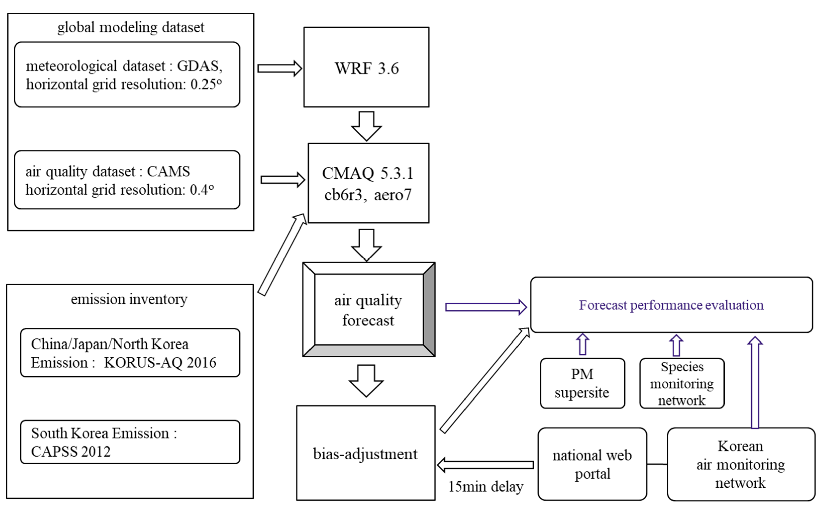
2.1. GMAF Configuration and Input Data

As shown in Figure 1, the GMAF is configured with two nested domains. The outer domain consists of 178 × 128 horizontal grids with 27 km spacing that cover Korean peninsula, most of China, Japan and parts of Russia, while the inner nest consists of 67 × 82 horizontal grids with 9 km spacing that cover South Korea, parts of North Korea and parts of Japan. A hybrid, sigma-pressure vertical coordinate was used with 23 levels and the top level was located at 200 hPa.
As shown in Figure 2, the GMAF imported CMAQ [23] for air quality forecast and analysis. The CMAQ version 5.3.1 was used with the carbon bond version 6 mechanism [24] as a gas-phase chemical mechanism, which includes 77 chemical species and 218 chemical reactions. The aerosol dynamics were modeled by AERO7 module, which includes 16 inorganic aerosol species, 33 organic aerosol species, as described in the github of CMAQ website [25]. The CMAQ divides sea salt into individual inorganic aerosol species and includes them except the coarse mode cations. Similarly, the CMAQ divides dust into individual aerosol species except the unknown composition fraction. The CMAQ treats the coarse mode cations of sea salt and the unknown composition fraction of dust as lumped aerosol species. The below-cloud scavenging module and the secondary organic aerosol formation mechanism were modified, and the evaporation loss of nitrate was added as detailed in Section 2.4. The WRF-ARW model version 3.6 [26] was used to provide the values of meteorological variables to the CMAQ.
Global assimilated datasets were used for generation of initial and boundary conditions of the outer domain and for providing gridded data to the grid nudging based FDDA. The WRF used the 0.25° global data assimilation system (GDAS) dataset and the CMAQ used the 0.4° CAMS dataset. The CAMS dataset was produced by the ECMWF’s IFS using four-dimensional variational data assimilation of the polar orbiting satellite data. A hybrid, sigma-pressure vertical coordinate was used with 137 levels and the top level was extended to 0.01 hPa. The CAMS dataset provided the concentration of 14 gaseous species and seven aerosol species in 3 h intervals [27]. The gaseous species were nitric oxide (NO), nitrogen dioxide (NO2), sulfur dioxide (SO2), formaldehyde (HCHO), ozone (O3), peroxyacetyl nitrates (PAN), hydrogen peroxide (H2O2), nitric acid (HNO3), hydroxyl radical (OH), carbon monoxide (CO), methane, ethane, propane, and isoprene. The aerosol species were dust, sea salt, hydrophobic black carbon, hydrophilic black carbon, hydrophobic organic matter, hydrophilic organic matter, and sulfate. The dust and the sea salt were distributed into the three size bins: 0.030–0.55, 0.55–0.9 and 0.9–20 µm for the dust and 0.03–0.5, 0.5–5 and 5–20 µm for the sea salt.
The clean air policy support system (CAPSS) emission inventory [28] was used to generate the gridded anthropogenic emission of South Korea. The Korea–United States air quality study (KORUS-AQ) anthropogenic emission inventory [29] was used for the rest of the region. The biogenic emissions were generated by MEGAN version 2.1 [30]. The CAPSS emission inventory is a national emission inventory compiled and published annually using the estimated or directly monitored emissions of CO, NO2, SO2, total suspended particulate (TSP), PM10, PM2.5, black carbon (BC), volatile organic compound (VOC), and ammonia (NH3) from the point, the area and the mobile sources. The KORUS-AQ emission inventory was constructed from the CREATE emissions [31] to support the KORUS-AQ field campaign carried out in the spring of 2016.
The bias adjustment technique was applied to remove the bias of PM2.5 forecast using the previous days’ PM2.5 observation and forecast. The GMAF retrieved the hourly PM2.5 measurements from the criteria air pollutant monitoring network with a 15 min delay. The collected hourly measurements were averaged at the end of the day to calculate the daily mean PM2.5 concentration for the use of bias adjustment.
The three air monitoring networks in Korea measure the PM2.5 and related species. Those are the criteria air pollutant monitoring network, the PM2.5 speciation monitoring network and the PM2.5 supersites. The criteria air pollutant monitoring network, consisting of 264 urban sites, 19 rural sites, three background sites as of 2016, measures the criteria air pollutant concentration including PM2.5 mass concentration. The PM2.5 speciation monitoring network and the PM2.5 supersites measure the PM compositions such as sulfate, nitrate, ammonium, organic carbon, elemental carbon, and mineral species. The PM2.5 compositions measured at the Bulkwang PM supersite were used for verification of the GMAF. The PM2.5 mass concentrations measured at the criteria air pollutant network were used to evaluate the GMAF using both the continuous forecast performance metrics and the categorical forecast performance metrics.

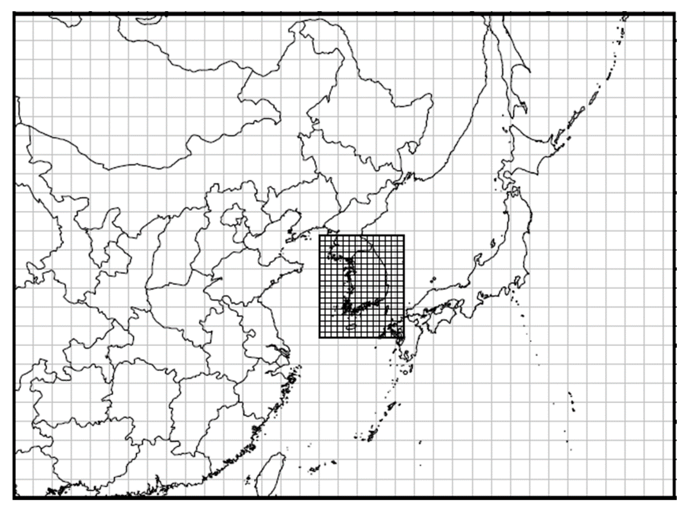
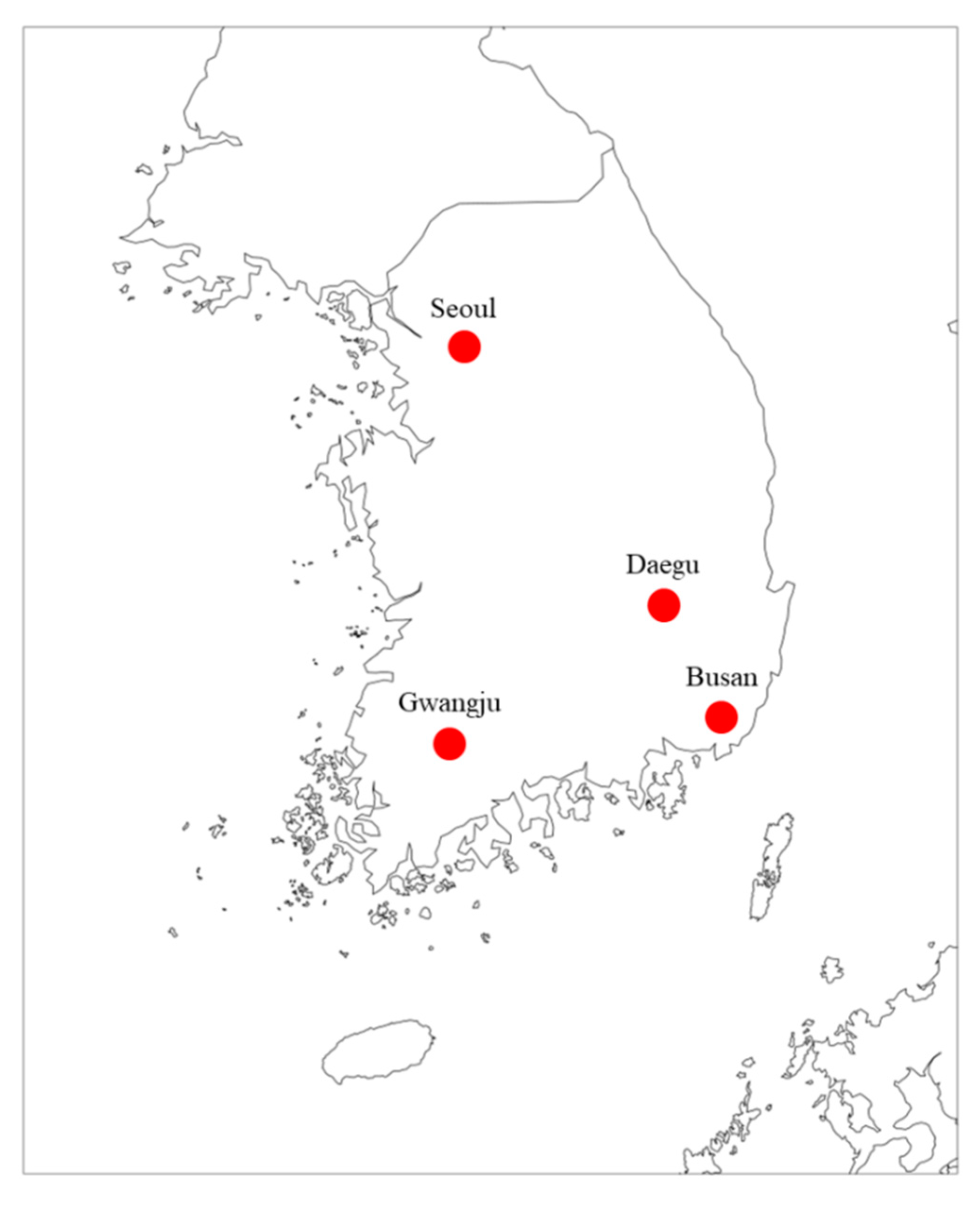
2.2. Forecasting Period and Area

The first national air quality standard for PM2.5 was promulgated in Korea in 2015 to begin installation of a PM2.5 monitoring instrument at the criteria air pollutant monitoring station. Most of the criteria air pollutant monitoring stations in the urban area were equipped with a PM2.5 monitoring instrument by 2016. Furthermore, KORUS-AQ field campaign was conducted in the spring of 2016 to provide the measurements from aircraft, ground sites and ships. The KORUS-AQ emissions were also developed to support the campaign [32]. Taking into account availability of monitoring data and emission inventory, this study chose the period from December of 2015 to November of 2016 for verification and evaluation of the GMAF. Four major cities in Korea were selected as target areas. Those are Seoul, Busan, Gwangju, and Daegu as displayed in Figure 3.
The PM2.5 pollution in Seoul and Busan expressed in Figure 4, the first and second largest city in Korea, was the worst in 2016 in the period from 2015 to 2019. As shown in Table 1, the annual mean PM2.5 concentration was the highest and the number of days exceeding the PM2.5 standard of 35 μg/m3 was the largest in 2016. Among meteorological parameters, precipitation, wind velocity and wind direction affect the year-to-year variations of the PM2.5 concentrations the most. The precipitation from June to September of 2016 was 52% less than the 30-year average in Seoul. This low precipitation reduced the wet scavenging to increase the PM2.5 concentrations. The PM2.5 concentrations from June to September of 2016 were higher than the other year averages of the same period by 33%. The number of days of exceeding the PM2.5 standard of 35 μg/m3 from June to September of 2016 was larger than the other year averages of the same period by 258% in Seoul as shown in Figure 4.
Busan is located about 320 km southeast of Seoul. The observed precipitation from May to August in 2016 was comparable to the 30-year average in Busan, and therefore the precipitation is unlikely to contribute to the PM2.5 increase. Instead, the stagnant wind conditions that occurred in November 2016 increased the monthly mean concentrations and the number of days of exceedances as shown in Figure 5.

2.3. Grid Nudging Based FDDA Method

Data assimilation combines model with observation to improve performance of the forecast and the reanalysis [33]. The grid nudging based FDDA adds a relaxation term that is supposed to force the observations to the model [34] as
d Y m o d e l dt = F ( x , Y m o d e l ) + W ( x ) ( Y obs Y model )
where Y is the dependent variable, F is a discretized form of the governing equation, x is the independent spatial variable, and W is the nudging coefficient. The subscripts ‘obs’ and ‘model’ denote the observations and the model, respectively. Global assimilated datasets may be used instead of observations to combine the mesoscale model with the global model. The dependent variables, Y, are defined as
Y =   α ( p t p s )   for   the   WRF ,
Y =   φ J s   for   the   CMAQ ,
where α is the meteorological variable of the WRF, φ is the chemical species concentration, pt is the air pressure at the top of the domain, ps is the air pressure at the surface and J s is the vertical Jacobian of the terrain-influenced coordinates. The variables nudged for the WRF were U, V winds, temperature and water vapor mixing ratio. The water vapor mixing ratio in the PBL and the surface temperature were not nudged. The nudging coefficients used for the WRF in this study were set as recommended by Baker et al. (2009) [35] and listed for completeness in Table 2.
The nudged variables of the CMAQ were selected to be consistent with CAMS dataset. The primary pollutants were selected to minimize the emission uncertainties in the outer domain. The O3 was added to the FDDA nudged variable list because its satellite observation data which the CAMS based on were reasonably accurate. In addition, the grid based FDDA on O3 enables incorporation of stratospheric intrusion into the mesoscale model domain. The grid spacing of the CAMS dataset is 0.4° (about 40 km in mid-latitudes) and the grid spacing of outer domain and inner nest of the GMAF are 27 and 9 km, respectively. Interpolation of the CAMS dataset to the inner nest may severely underestimate the peak values due to a large difference between the grid resolutions. Moreover, the emission uncertainties in the inner nest, Korea emission, were reasonably small. Therefore, the grid nudging based on FDDA was applied only to the outer domain. Table 2 presents the list of nudged chemical species with the corresponding nudging coefficients.

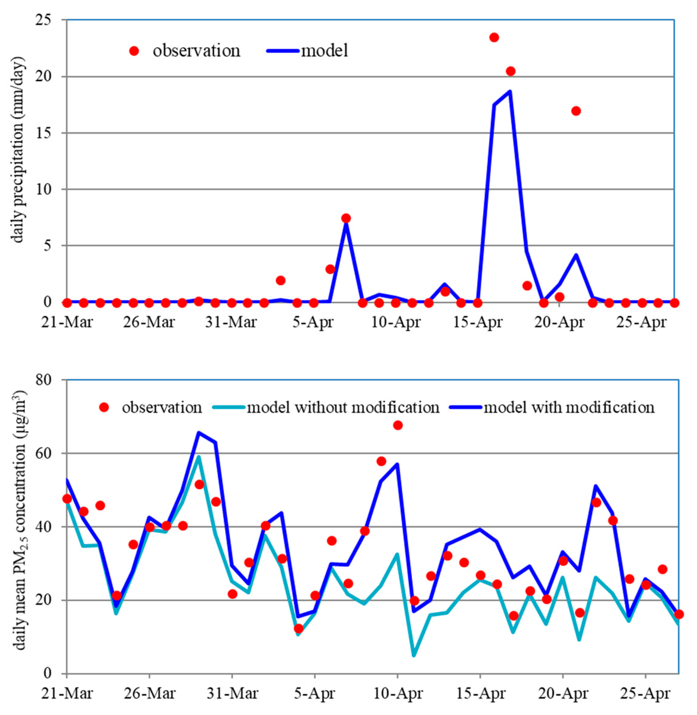
2.4. Modification of the CMAQ

The CMAQ was modified to enhance the model accuracy based on the recent findings deduced from model verification as described below.

2.4.1. Below-Cloud Scavenging

The CMAQ assumes that accumulation mode and coarse mode particles are completely absorbed into cloud and rainwater. This assumption is valid only for a cloud environment where water droplets are readily formed around particles due to high water vapor contents but not valid for a rain environment. It may lead to overestimation of below-cloud scavenging and subsequently to underestimation of particulate matter concentrations in the below-cloud region.
In order to remove the complete absorption assumption in a rain environment, the CMAQ was modified to calculate the below-cloud scavenging rate by
c ( t ) t = Λ c ( t )  
where c(t) is the particulate species concentration at time t and the Λ is the scavenging coefficient [36]. The below-cloud scavenging coefficient was calculated by semiempirical formula derived by Slinn (1983) [37] with the empirically estimated mean raindrop diameter [38]. The calculated below-cloud scavenging coefficients ranged 10−6~10−2 s, consistent with the field measurements [39].
If the particles are completely absorbed into rainwater as the CMAQ assumes, then the below-cloud scavenging coefficient should be equal to 1, which is several orders of magnitude larger than the one estimated here. More importantly, it remains constant whereas it should increase with the precipitation intensity. As a result, the CMAQ seriously overestimates the below-cloud scavenging rate and subsequently underestimates PM2.5 concentration especially when the precipitation intensity is low.
The WRF-CMAQ simulation was performed from 21 March to 27 April in 2016 to test the modified below-cloud scavenging module. Figure 6 compares the modeled and observed precipitations at Seoul. The modeled and observed surface PM2.5 concentrations were also compared. The modeled precipitation agrees very well with the observation except 21 April. The dates of the modeled precipitation between 0.1 mm/day and 1.0 mm/day are 29, 30 March, and 3, 6, 8, 9, 10, 14, 19, 22 April. As also shown in Figure 6, the CMAQ without modification considerably underestimated the PM2.5 concentrations on these dates of little precipitation. As noted earlier, this is because the CMAQ severely overestimated the below-cloud scavenging rates by assuming complete absorption of particles into rainwater. The CMAQ with the proposed modification reduced overestimation of the below-cloud scavenging rates, resulting that the modeled PM2.5 concentration agreed well with the observation.

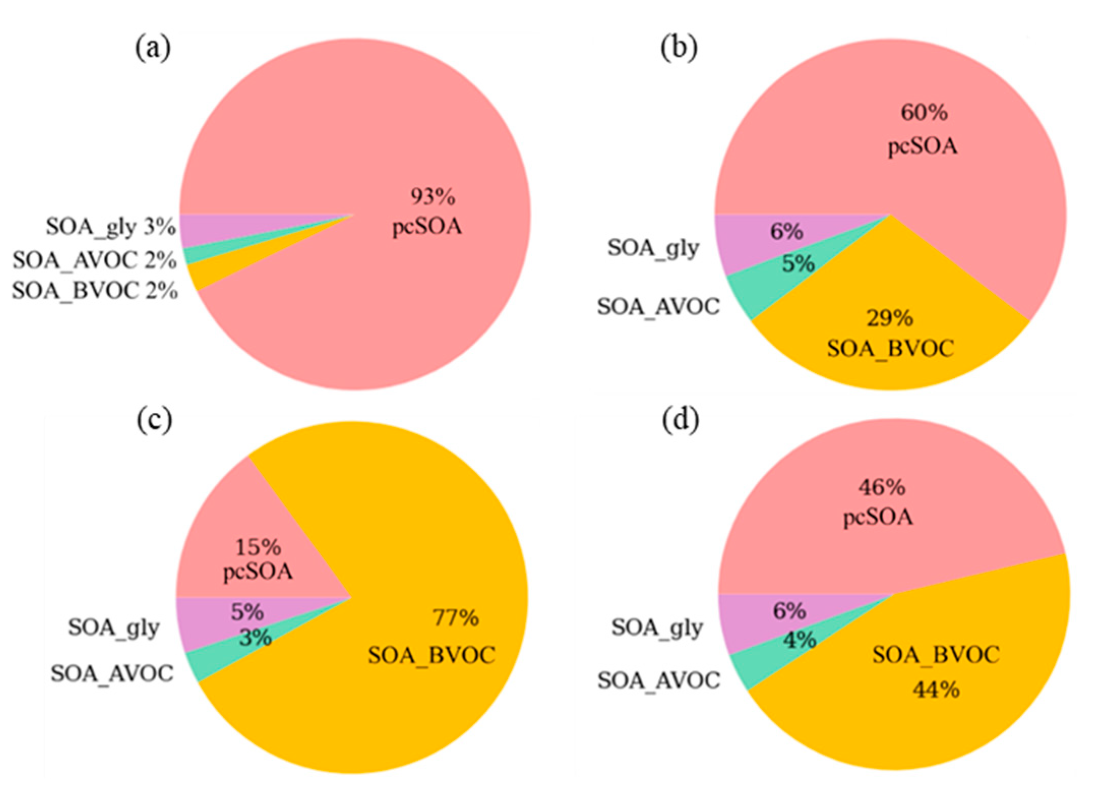
2.4.2. Secondary Organic Aerosol Formation

In the present study, the AERO7 module including 12 primary organic aerosols (POA) and 21 secondary organic aerosols (SOAs) were used to model SOA formation. Compared to the previous versions of aerosol module, the AERO7 module expanded the SOA formation mechanism by adding pcSOA, organic nitrates from monoterpene oxidation and SOA from glyoxal and methylglyoxal. The pcSOA, standing for the potential SOA from combustion emissions, is a surrogate species designed to compensate missing and underestimated mass from combustion.
The pcSOA production rate of the AERO7 module was optimized for the southern and northern California sites and was known to overestimate the SOA in the continental US application [40]. Figure 7 displays the model calculated SOA compositions by season in Seoul. Here, the SOA was divided into four groups, pcSOA, SOA from biogenic VOCs (SOA_BVOC), SOA from anthropogenic VOCs (SOA_AVOC), and SOA from glyoxal and methylglyoxal (SOA_gly) for convenience. The pcSOA was the most dominant SOA in the winter due to low temperatures whereas the SOA_BVOC was the most dominant SOA in the summer due to high emission fluxes of biogenic VOCs and fast photochemical production. These seasonal characteristics of SOA compositions appeared similarly in most urban areas in Korea.
The CMAQ with the AERO7 module considerably overestimated the PM2.5 mass in the winter. As the pcSOA was a dominant species in the winter, the PM2.5 overestimation might be lessened by adjusting the pcSOA concentration by multiplying the pcSOA weighting factor (PWF). As shown in Figure 8, the AERO7 module with the PWF of 1.0 overestimated the observed monthly mean PM2.5 concentrations at Seoul by 12~49%. As the PWF decreased to 0.4 and to 0.0, the modeled PM2.5 concentrations were getting smaller. The modeled monthly mean PM2.5 concentrations best agreed with the observations when the PWF was set to 0.4.
In addition, we conducted statistical performance evaluation to search an optimum value of the PWF. As listed in Table 3, the model performances in PM2.5 forecast at four major cities in Korea in 2016 were evaluated by correlation coefficient (R), normalized mean bias (NMB), normalized mean error (NME), probability of detection (POD), false alarm ratio (FAR), and Heidke skill score (HSS), the definition and the usage of which were presented in Section 2.6. As the PWF increased, the R increased indicating performance improvement. However, there was no clear relation between the PWF and the NME. The POD increased with the PWF indicating performance improvement whereas the FAR decreased with the PWF indicating performance decline.
The R, the NMB, the NME, the POD, and the FAR are simple statistical metrics evaluating a partial performance of the model and therefore they may not agree with each other as happened here. This study used the HSS to decide an optimum value of the PWF, because the HSS evaluates the overall performance. The HSS averaged over the four cities was the highest when the PWF was equal to 0.4 or 0.7. The HSS at Seoul, the most populated city in Korea, was the highest when PWF was equal to 0.4. This value of the PWF is the same as the value previously derived using Figure 8. Therefore, the PWF was set equal to 0.4 in this study.
The PM supersite located at Bulkwang in Seoul collected PM2.5 on a quartz filter every three days and analyzed them for organic carbon (OC). The observed OC at the Bulkwang PM supersite was compared with the modeled OC in Figure 9. The CMAQ calculated organic matter (OM) concentrations instead of OC concentrations. Therefore, the calculated OM concentrations were converted to the OC concentrations by taking account of molecular formula of individual organic aerosol species constituting the OM. As shown in Figure 9, the modeled OC agreed well with the observation except the summer. As the pcSOA dominated except the summer, the model must have accurately estimated the pcSOA concentration with the PWF of 0.4.
One other thing to note is that the model significantly over-predicted the OC in the summer. As most of SOA in this period is the SOA from biogenic VOCs as shown in Figure 7, it is highly likely that the emissions of biogenic VOCs, isoprene and terpenes were overestimated or that the conversion rates from the biogenic VOCs to the SOA were overestimated. More studies are necessary to address this over-prediction problem.

2.4.3. Evaporation Loss of Nitrate

A national reference method for PM2.5 in many countries including Korea specifies Teflon membrane filter for collection of ambient particles. Teflon membrane filter may cause a significant evaporation loss of particulate nitrate (NO3) during and after the sampling in the warm environment [41,42]. Assuming equilibrium, the evaporation loss ( Δ NO 3 ) is expressed as
Δ NO 3 = 745.7 T R i = 1 i = 24 K i 24 ,
where TR is the daily average temperature of the sampled air and Ki is the dissociation constant for ammonium nitrate evaluated at the ambient temperature and the relative humidity for hour i as described by Frank (2006) [43].
The GMAF applied Equation (5) to the temperature and humidity calculated by the WRF to estimate the nitrate evaporation loss. The estimated nitrate evaporation loss was subtracted from the nitrate concentration calculated by the CMAQ to estimate the nitrate concentration left on the filter after evaporation.

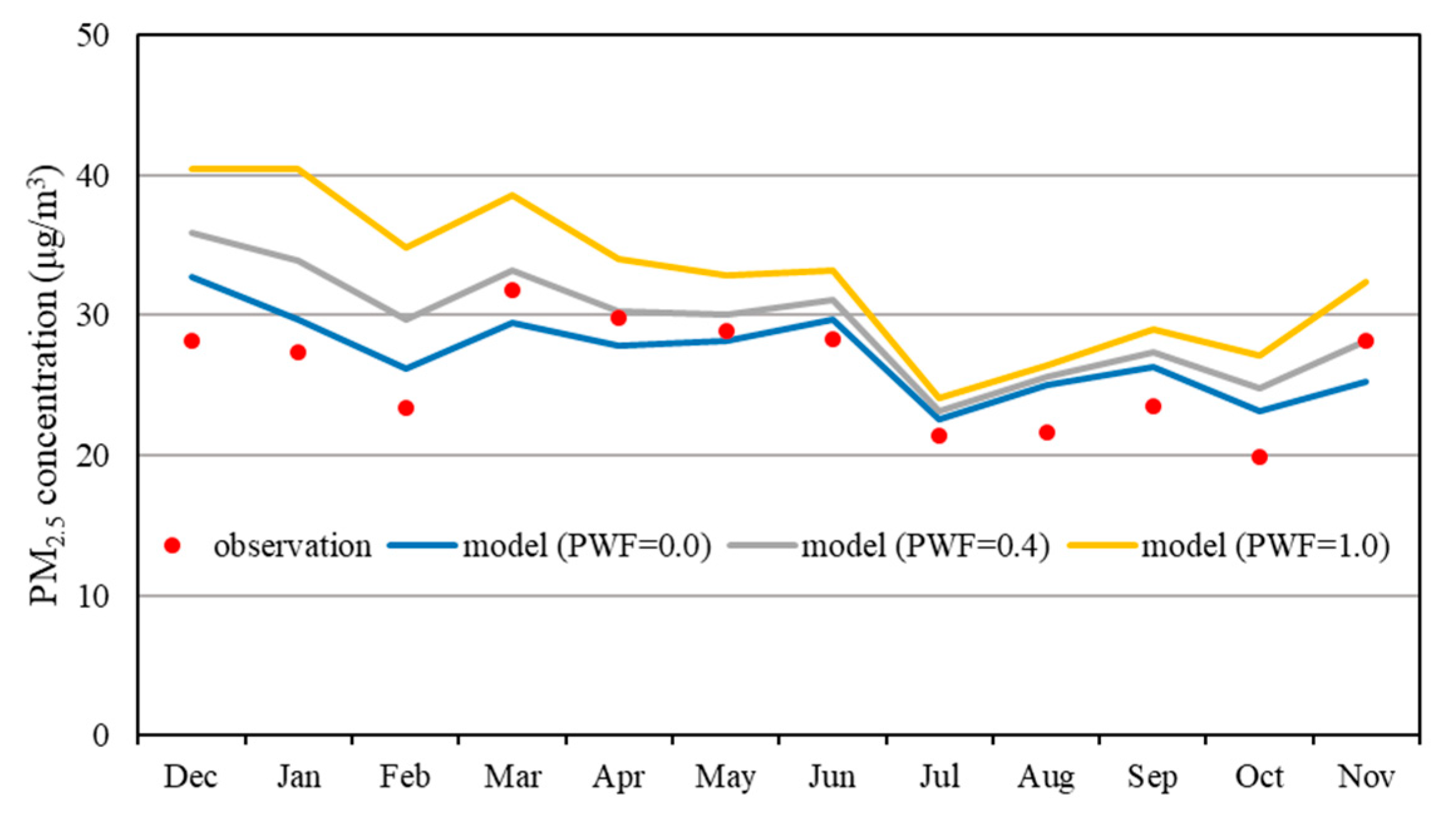
2.5. Implementation of Bias Adjustment Techniques

The accuracy of air quality forecast may be improved by applying bias adjustment techniques. Both the hybrid bias correction technique and the Kalman filter bias adjustment technique were implemented into the GMAF as postprocessors. The hybrid bias correction technique uses either the difference or the ratio between the forecast and the observation [44]. The former is an additive correction and expressed as
C t + Δ t =   F t + Δ t + 1 Nday   j = Nday 1 j = 0 ( O t j Δ t F t j Δ t ) .
The latter is a multiplicative correction and expressed as
C t + Δ t =   F t + Δ t × j = Nday 1 j = 0 O t j Δ t j = Nday 1 j = 0 F t j Δ t ,
where C is the corrected forecast value, F is the raw forecast value and O is the observation. Nday denotes the number of previous days representing a training period. Typical values for Nday are the numbers between 1 and 5.
Kalman filter bias adjustment technique predicts the future bias by correcting the previous estimate of the bias using the difference between the bias estimate and the forecast error at the previous time. The predicted future bias is used to adjust the forecast. The Kalman filter bias adjustment technique was implemented into the GMAF by following the work by Delle Monache et al. (2006) [22]. Kalman filter bias adjustment technique is sensitive to the error ratio, which determines the relative weighting between the observation and the forecast and needs to be optimized.

2.6. Forecast Performance Evaluation Metrics

The methods for forecast performance evaluation are introduced in this section. Selected forecast period and variables for forecast evaluation are also discussed.

2.6.1. Forecast Variables

The GMAF can forecast most of the criteria air pollutants but this study selected the PM2.5 for performance analysis. As of 2016, 25 PM2.5 monitoring stations were located in Seoul, 19 stations in Busan, six stations in Gwangju and seven stations in Daegu. Korea uses the PM2.5 concentration averaged over all the stations in the city of interests to set a policy goal and to calculate the air quality index (AQI). Taking averages over the city improves the spatial representativeness of monitoring data and reduces the associated errors.
Although the recent advances in analytical chemistry have made it possible to measure PM2.5 mass and composition at time intervals equal to or less than 1 h, most of PM2.5 toxicity and PM2.5 management studies still use the daily mean or annual mean concentrations as a metric of PM2.5. This study used the daily mean PM2.5 concentration for forecast performance evaluation.

2.6.2. Performance Evaluation Metrics of Continuous Forecasts

Continuous forecast aims at forecasting the values of continuous variables. Temperatures, wind velocities and air pollutant concentration are good examples of continuous variables. The model performance of continuous forecast was measured by three statistical metrics in this study; R, NMB and NME. The R, correlation coefficient, gives a measure of linear relationship between two variables and ranges between −1 and 1. The R between the forecast and observed values is defined as
R = i = 1 i = N ( O i O ¯ ) ( F i F ¯ ) i = 1 i = N ( O i O ¯ ) 2 i = 1 i = N ( F i F ¯ ) 2 ,
where Oi and Fi are the observation and the forecast, respectively, and N is the number of paired data sets.
The NMB, normalized mean bias, is the difference between observed and forecasted mean value normalized by the observed mean value and is defined by
NMB = F ¯ O ¯ O ¯ × 100 .
The NMB is a useful metric for measuring the systematic errors. However, as the number of datasets increases, under-forecasted values tend to offset over-forecasted values to improve the NMB even if the accuracy remains unchanged. The root mean square (RMSE) uses the square of the difference between the observed and forecasted value to measure the errors as defined by
RMSE = 1 N i = 1 i = N ( F i O i ) 2 .
The squaring operation makes the RMSE strongly dominated by the largest errors. The RMSE is not recommended for the air quality forecast and analysis because of its high sensitivity to the largest concentrations [10,45].
The normalized mean error (NME) uses the absolute value of the difference instead of the squares of them as defined by
NME   = 1 N i = 1 i = N | F i O i | O ¯ × 100 .
The NME gives a measure of the overall forecast error and is used in this study instead of RMSE.
Emery et al. (2017) [45] analyzed the model performance evaluation studies published from 2006 to 2012 in the United States and recommended the criteria and goal of the R, the NMB and the NME as listed in Table 4, which is used in this study as a reference.

2.6.3. Performance Evaluation Metrics of Categorical Forecasts

Categorical forecast aims at forecasting the occurrence of a specific event. The event of interests in this study is that the PM2.5 concentration exceeds the Korean PM2.5 standard of 35 μg/m3. The contingency table used for analysis of the relationship between two categorical variables is presented in Table 5, where the “A” is the number of event forecasts with event occurring. The “B” is the number of event forecasts with event not occurring. The “C” is the number of no-event forecasts with event occurring. Finally, the “D” is the number of no-event forecasts with event not occurring.
The A, B, C, D in the contingency table may formulate various performance metrics, including probability of detection (POD), probability of false detection (PODF), false alarm ratio (FAR), success ratio (SR), critical success index (CSI), true skill statistic (TSS), Gilbert skill score (GS), Heidke skill score (HSS), bias (B), and accuracy (A) [46].
The POD ranges from 0 to 1 with 1 being a perfect forecast and is defined by
POD =   A ( A + C ) .
The POD considers missed events only, neglecting false alarms and therefore it can be artificially improved by over-forecasting. The FAR complements the POD in this aspect and is defined by
FAR =   B ( A + B ) .
The FAR ranges from 0 to 1 with 0 being a perfect forecast. The FAR considers false alarm events only, neglecting missed events and therefore it can be artificially improved by under-forecasting.
The POD and the FAR are examples of simple skill metrics. The problem of simple skill metrics is that a good score does not necessarily mean a good overall forecasting performance. One can overcome this problem by combining two or more simple skill metrics. This kind of skill metrics, called here as complex skill metrics, are the CSI, the TSS and the HSS. The CSI and the TSS may not work properly for rarely occurring events. As exceedance of the PM2.5 standard, the event in this study, may occur rarely in certain seasons and regions, we selected the HSS as a complex skill metric.
The HSS is the fraction of accurate forecast with correction of random forecasts as defined by
HSS =   A + D E A + B + C + D E ,
where E is the number of correct random forecasts as defined by
E =   ( A + B ) ( A + C ) + ( B + D ) ( C + D ) A + B + C + D .
The HSS ranges from −∞ to 1 with 1 being a perfect forecast. The HSS above zero means that the forecast is better than a random guess and the HSS above 0.5 is deemed a good score.
Studies on categorical forecast performance evaluation of PM2.5 forecast were much more limited than studies on continuous forecast performance evaluation [47]. The POD for the event of exceeding the 8-h O3 standard in the Northeastern United States ranged between 0.07 and 0.37 whereas the FAR, often larger than the POD, ranged between 0.64 and 0.76 [48]. The POD for the event of exceeding the 24-h PM2.5 standard in the Eastern United States was 0.28 whereas the FAR was 0.35 [49]. The POD for the event of exceeding the 24-h PM2.5 standard in Korea ranged between 0.1 and 0.39 whereas the FAR ranged between 0 and 0.64 [50].

3. Results and Discussion

The performance evaluation results of the GMAF are presented in this section. Test results of performance improvement attained by incorporating the nitrate evaporation and the bias adjustment techniques are also presented.

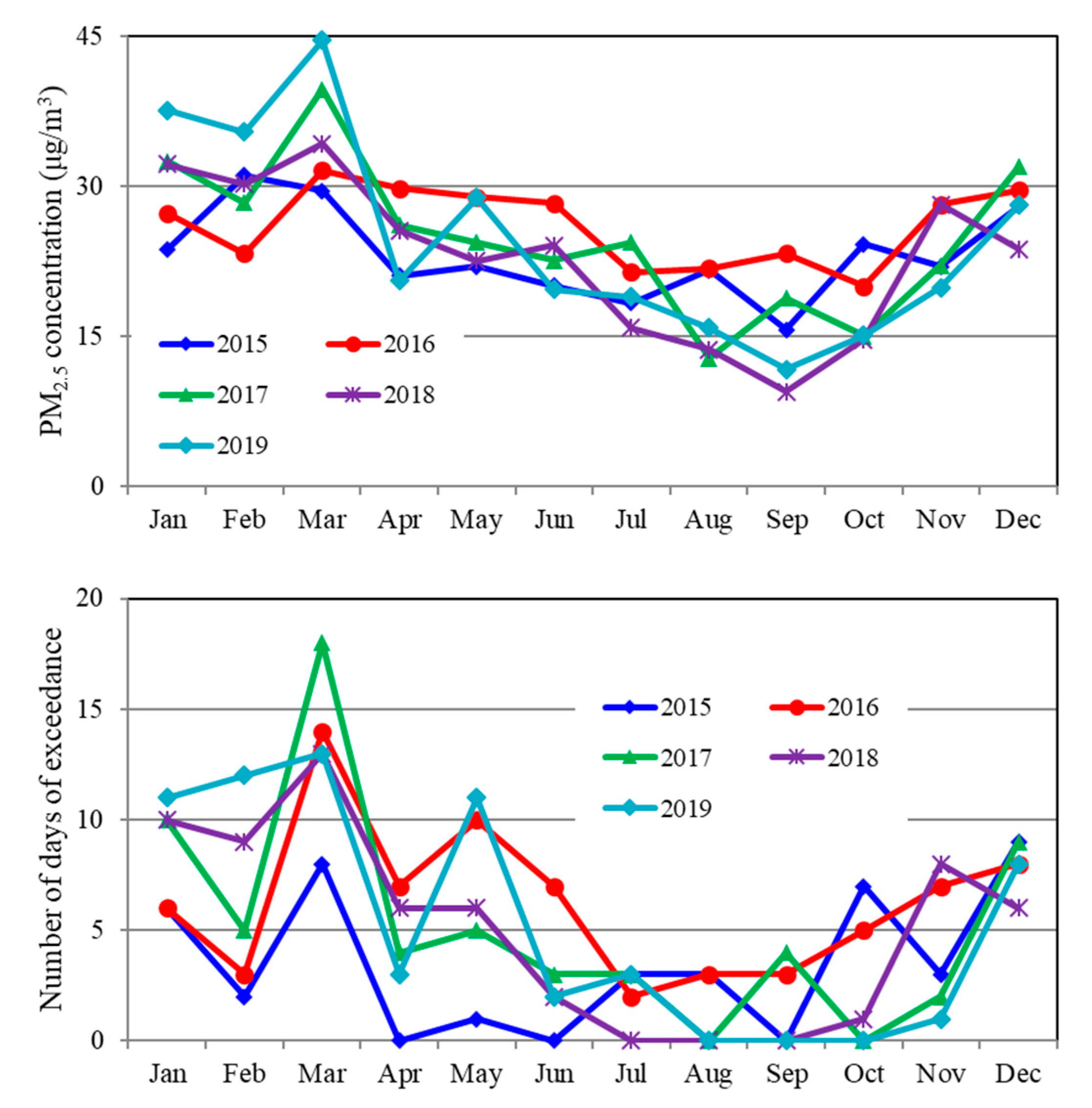
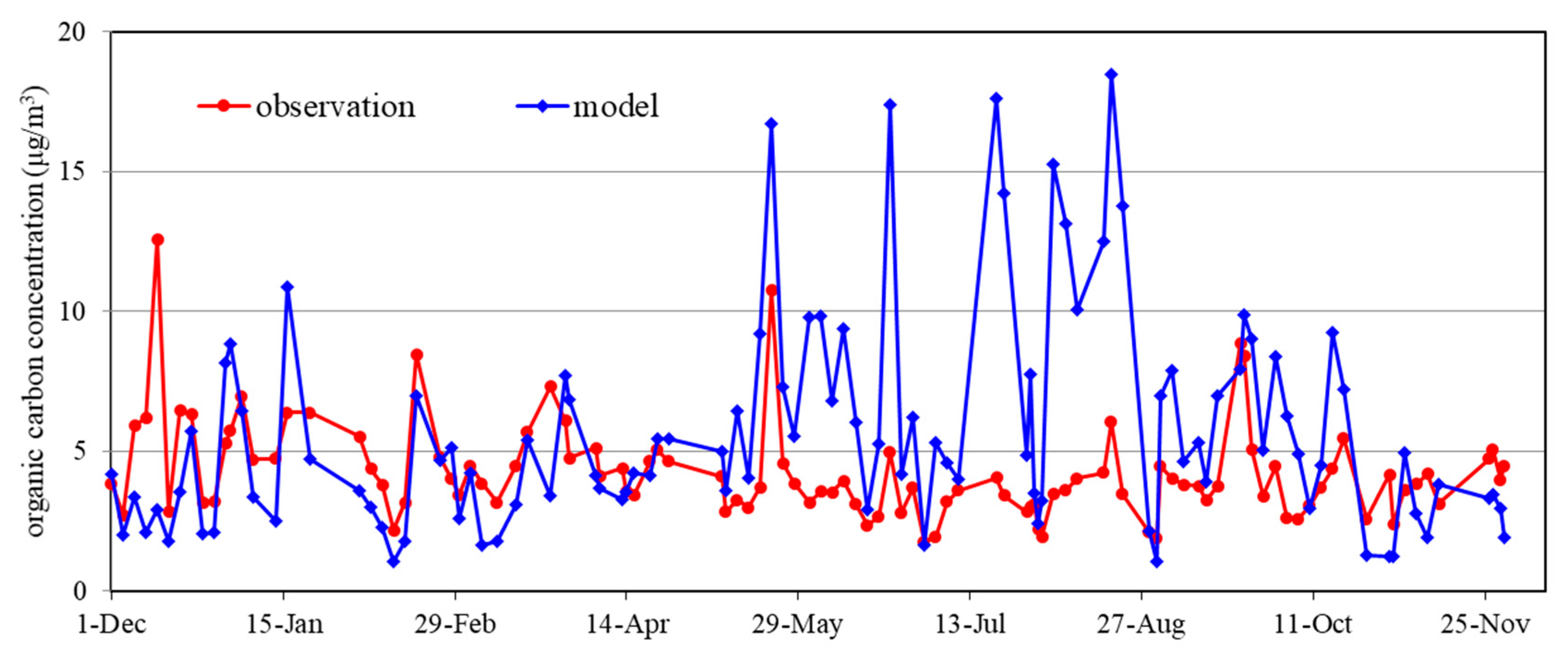
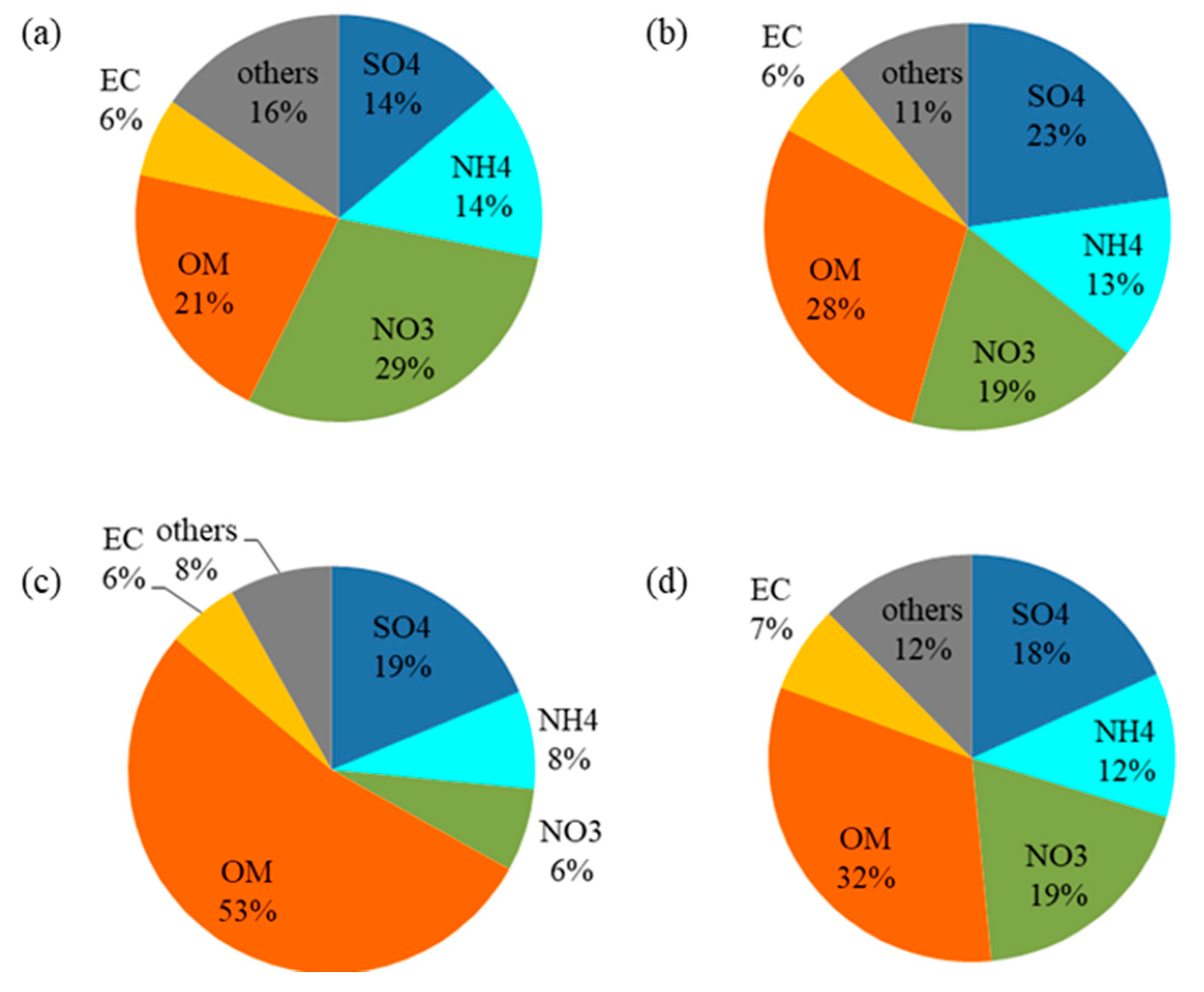
3.1. Performance Evaluation of the Base Forecast

The GMAF was used to forecast the PM2.5 for the year 2016. All the modifications described in Section 2.4 were included except nitrate evaporation loss. Table 6 shows the seasonal and yearly values of performance metrics, where the seasons were defined as winter (December, January, February), spring (March, April, May), summer (June, July, August), and fall (September, October, November). The average PM2.5 concentrations in the winter and the spring were higher than those in the summer and the fall in all the four selected cities, which are very typical of the PM2.5 concentrations in Korea. The annual values of R were higher than 0.78 in all four cities, satisfying the goal set in Table 4. The winter values of R were the higher than the other seasons and the summer values of R were lower than the other seasons except Busan.
The NMBs at Seoul were positive in all the seasons, indicating over-forecasting, whereas those at Busan were all negative, indicating under-forecasting. Out of total 16 cases (four seasons and four cities), half of the cases had the NMB value less than ±10%, achieving the goal set in Table 4 and the other half of cases had the NMB value less than ±30%, satisfying the criteria also set in Table 4. The seasonal NME ranged between 19% and 27%, achieving the goal set in Table 4. Unlikely to the R, the NME did not exhibit a distinctive seasonal variation.
The number of days exceeding the 24-h PM2.5 standard, which is the frequency of occurrence of events, ranged between 17 and 31 days during the winter and the spring because of severe PM2.5 pollution in Korea. The frequency of occurrence of events in this study is several times higher than that in the literature quoted in Section 2.6.3. It may be noted here that categorical forecasts perform better for the frequent events than for the rare events. During the winter, the skill scores were very good; the POD were 0.68~1.0 and exceeded the FAR by 0.41~0.59, and HSS were 0.58~0.68. Although the skill scores went down in the spring and fall, all three skill scores were still deemed fairly good.
The categorical forecast performed poorly during the summer compared to the other seasons because of two reasons. Firstly, as noted above, the R values and the NME values in the summer were generally lower than those in the other seasons, indicating the GMAF might not perform well in the summer. Secondly, the events occurred less frequently in the summer due to lessened PM2.5 pollution in Korea, which might worsen the categorical skill scores measured by the POD, the FAR and the HSS.
As discussed above, both the GMAF performed the best during the winter and worst during the summer. In order to investigate the effects of seasons on the forecast performance, the modeled seasonal PM2.5 chemical compositions are displayed in Figure 10. The nitrate was a dominant PM2.5 species in the winter. The PM2.5 nitrate in the urban area is rather locally produced than regionally transported [51]. The local emissions of nitrogen oxides (NOx) were well known and the homogeneous and heterogeneous chemical pathways were well defined such that the GMAF was able to accurately predict the PM2.5 nitrate concentrations and subsequently the PM2.5 mass concentrations during the winter.
During the summer, the PM2.5 mass was dominated by the OM, the most of which was the SOA from biogenic VOC as shown in Figure 7. There was large uncertainty in estimating biogenic VOC emission and in modeling aerosol formation processes from biogenic VOCs, which probably degraded the model performance.

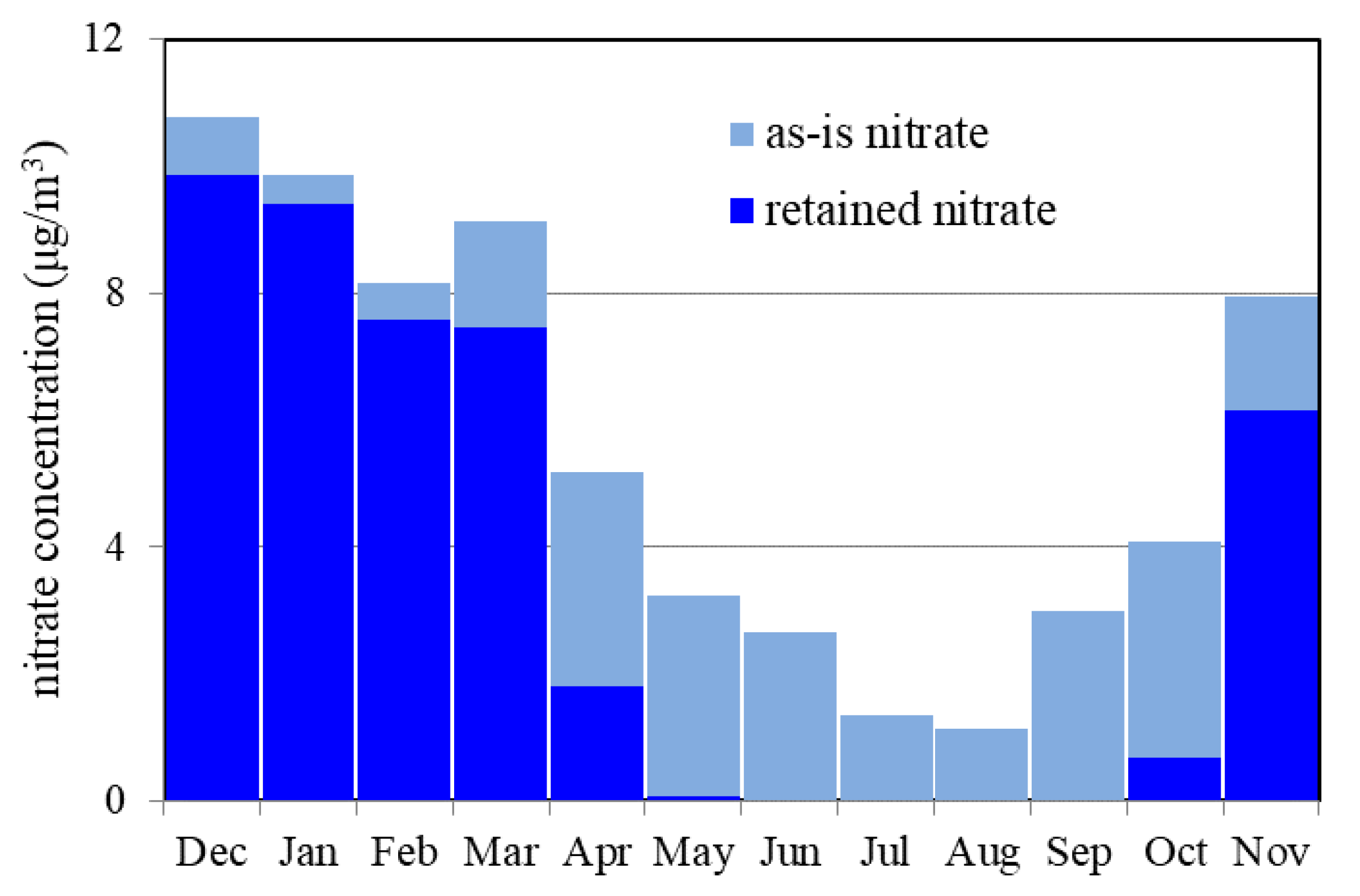
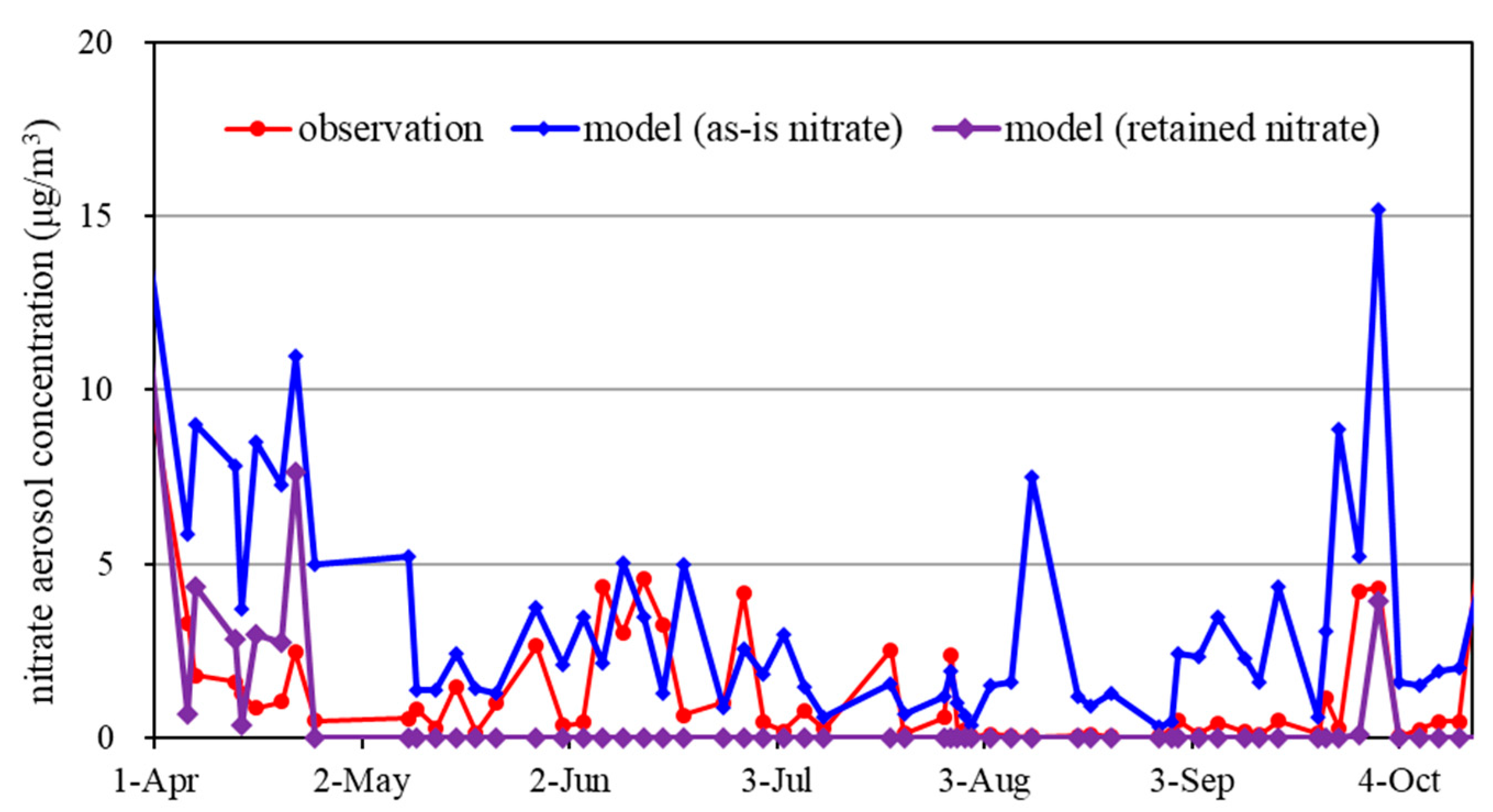
3.2. Modeling of Nitrate Evaporation Loss

The PM supersite located at the Bulkwang in Seoul measured the PM2.5 mass and PM2.5 nitrate using Teflon membrane filter. Teflon membrane filter causes a significant evaporation loss of particulate nitrate during and after the sampling in the warm environment. Here, the nitrate before evaporation loss is defined as as-is nitrate, whereas the nitrate left on the filter after evaporation loss is defined as retained nitrate.
The monthly mean concentrations of the retained nitrate at the Bulkwang site were calculated by applying Equation (5) to the temperature and the humidity forecasted by WRF and the nitrate concentration modeled by CMAQ. As displayed in Figure 11, both the as-is and retained PM2.5 nitrate concentration were the highest during the winter months and the lowest during the summer months because the ratios of nitrate aerosol to nitric acid gas (NO3/HNO3) decrease with temperature increase. In the summer months, the nitric acid mainly stayed in the gas phase due to the warm temperature. It may be noted that the nitric acid gas is readily removed by wet and dry deposition to have shorter lifespan than the nitrate aerosol.
The difference between as-is nitrate and retained nitrate is the evaporation loss of nitrate taking place during and after Teflon filter sampling. The evaporation loss is less than 10% of as-is nitrate during the winter months whereas it was more than 80% of as-is nitrate during the summer months. Therefore, the retained nitrate was negligibly small by being less than 0.5 μg/m3 during the summer months.
Figure 12 compares the observed nitrate with the modeled nitrate between April and October during which Equation (5) predicted a significant evaporation loss of nitrate as shown in Figure 11. As the nitrate was measured every three days, the modeled nitrate concentrations were also selected every three days in the Figure 12. The modeled retained nitrate agreed well with the observed nitrate in April, August, September, and October, indicating that Equation (5) calculated the nitrate evaporation loss accurately. The retained nitrate concentrations were kept below 5 μg/m3 to lessen the nitrate overestimation appeared in the as-is nitrate concentration. However, the observed nitrate was closer to the modeled as-is nitrate than the modeled retained nitrate about half of May, June and July. This underestimation of the retained nitrate is probably due to inaccurate estimation of the temperature to which the nitrate evaporation loss is sensitive.
Table 7 shows the effect of inclusion of nitrate evaporation loss on the forecast performance in the spring and the fall during which the nitrate evaporation loss had a discernible effect on the PM2.5 mass concentration. The CTMs including the CMAQ are exposed to high degrees of uncertainty in modeling physical and chemical processes and in preparing input data such as emissions, meteorological parameters. Enhancement of one module does not necessarily mean improvement of the forecast performance. As the nitrate evaporation loss was included, the NMB decreased as expected. The R decreased in all the four cities for the spring whereas it increased in Gwangju and Daegu for the fall. The NME increased in most cases. Therefore, it may be concluded that the performance of the continuous forecast was not improved although the nitrate evaporation loss was included. Moreover, the categorical forecast measured by the POD, the FAR and HSS was declined in most cases considered here.

3.3. Application of Bias Adjustment Technique

The bias adjustment techniques described in Section 2.5 were applied to the PM2.5 forecasts at the four cities for the year 2016. We tested different values of the number of previous days (Nday) for additive and multiplicative bias correction and different values of the error ratio for the Kalman filter bias adjustment, and chose 2 as the number of previous days and 0.5 for the error ratio.
The additive and multiplicative bias correction techniques were designed to remove the biases by algebraic manipulation. They successfully eliminated the biases at all the four cities as shown in Table 8. However, the improvements of biases did not propagate to the other performance evaluation metrics. They did not generally improve the R and the NME except for Seoul. Moreover, they generally degraded the POD and the HSS.
Although the Kalman filter bias adjustment technique was less efficient in reducing the NMB than the additive and multiplicative bias correction techniques, it improved all the other performance metrics significantly. The averaged values over the four cities were improved by 5% for the R, 13% for the NME, 11% for the POD, 8% for the FAR, and 10% for the HSS.

4. Conclusions

The GMAF was developed by utilizing the currently available multiscale air quality modeling system and the global forecast and analysis dataset. The GMAF implemented the grid nudging based FDDA onto the CMAQ for the first time to take advantage of data assimilation done in the global modeling. Although the current forecast verification was limited to the next day forecast and analysis, the forecasting period can be extended up to five days permitted by the global forecast and analysis model without a significant loss of accuracies.
The GMAF lessened the tendency of underestimating the PM2.5 concentrations in the case of little precipitation by improving the below-cloud scavenging coefficient estimation. The CMAQ-5.3.1 with carbon bond version 6 mechanism and AERO7 module significantly enhanced the accuracy of nitrate formation rate calculation by updating homogenous reaction rate constants and heterogeneous reaction mechanism. The SOA formation mechanism was also expanded by adding pcSOA, organic nitrates from monoterpene oxidation and SOA from glyoxal and methylglyoxal. The expansion of the SOA formation mechanism amended the underestimation problem of SOA frequently found in the previous version. However, a comparison with the observations indicated that the pcSOA in the winter and the SOA from biogenic VOCs in the summer might be overestimated. A more refined estimation of the pcSOA emissions and more accurate modeling of biogenic VOCs are recommended as future studies.
A severe PM2.5 episode often arises in the winter and the spring in Korea. The Korea government agency relies on the numerical forecast during these PM2.5 season in issuing a PM2.5 advisory or warning to the people. The GMAF performed very well especially in the winter suiting the needs of the government. In the winter, the R between the observed and forecasted PM2.5 was 0.87, the POD for event exceeding the national PM2.5 standard was 1.00, and the FAR was only 0.48 at Seoul. The GMAF also showed good performance at the other three cities, Busan, Gwangju and Daegu.

Author Contributions

S.C. coded most of computer programs for the GMAF and wrote this paper, H.P. conducted the model simulation and analyzed the results, J.S. led the work on the bias adjustment technique, L.C. contributed to the forecast interpretation and performance evaluation. All authors have read and agreed to the published version of the manuscript.

Funding

This research was funded by Korea National Institute of Environmental Research, grant number: NIER-2019-01-02-047.

Institutional Review Board Statement

Not applicable.

Informed Consent Statement

Not applicable.

Data Availability Statement

Monitoring data were obtained from National Institute of Environmental Research (NIER) and are available from the authors with the permission of NIER.

Acknowledgments

The authors would like to thank the Korean institute of environmental research for providing the Korean monitoring network data for criteria pollutants and PM supersite data.

Conflicts of Interest

The authors declare no conflict of interest.

References

  1. Fay, J.A.; Rosenzweig, J.J. An analytical diffusion model for long distance transport of air pollutants. Atmos. Environ. 1980, 14, 355–365. [Google Scholar] [CrossRef]
  2. Van Dop, H.; De Haan, B. Mesoscale air pollution dispersion modelling. Atmos. Environ. 1984, 18, 545–552. [Google Scholar] [CrossRef]
  3. Pudykiewicz, J.; Benoit, R.; Staniforth, A. Preliminary results from a partial LRTAP model based on an existing meteorological forecast model. Atmos. Ocean 1985, 23, 267–303. [Google Scholar] [CrossRef]
  4. McRae, G.J.; Goodin, W.R.; Seinfeld, J.H. Development of a second-generation mathematical model for urban air pollution—I. Model formulation. Atmos. Environ. 1982, 16, 679–696. [Google Scholar] [CrossRef]
  5. Carmichael, G.R.; Peters, L.K. An Eulerian transport/transformation/removal model for SO2 and sulfate—I. Model development. Atmos. Environ. 1984, 18, 937–951. [Google Scholar] [CrossRef]
  6. Cho, S.-Y.; Carmichael, G.R. An evaluation of the effect of reductions in ambient levels of primary pollutants on sulfate and nitrate wet deposition. Atmos. Environ. 1989, 23, 1009–1031. [Google Scholar] [CrossRef]
  7. Carmichael, G.R.; Peters, L.K. A second generation model for regional-scale transport/chemistry/deposition. Atmos. Environ. 1986, 20, 173–188. [Google Scholar] [CrossRef]
  8. Chang, J.; Brost, R.; Isaksen, I.; Madronich, S.; Middleton, P.; Stockwell, W.; Walcek, C. A three-dimensional Eulerian acid deposition model: Physical concepts and formulation. J. Geophys. Res. Atmos. 1987, 92, 14681–14700. [Google Scholar] [CrossRef]
  9. Jacobson, M.Z. Development and application of a new air pollution modeling system—II. Aerosol module structure and design. Atmos. Environ. 1997, 31, 131–144. [Google Scholar] [CrossRef]
  10. Marécal, V.; Peuch, V.-H.; Andersson, C.; Andersson, S.; Arteta, J.; Beekmann, M.; Benedictow, A.; Bergström, R.; Bessagnet, B.; Cansado, A. A regional air quality forecasting system over Europe: The MACC-II daily ensemble production. Geosci. Model Dev. 2015, 8, 2777–2813. [Google Scholar] [CrossRef] [Green Version]
  11. Mai, X.; Ma, Y.; Yang, Y.; Li, D.; Qiu, X. Impact of grid nudging parameters on dynamical downscaling during summer over mainland China. Atmosphere 2017, 8, 184. [Google Scholar] [CrossRef] [Green Version]
  12. Bowden, J.H.; Otte, T.L.; Nolte, C.G.; Otte, M.J. Examining interior grid nudging techniques using two-way nesting in the WRF model for regional climate modeling. J. Clim. 2012, 25, 2805–2823. [Google Scholar] [CrossRef]
  13. Inness, A.; Ades, M.; Agusti-Panareda, A.; Barré, J.; Benedictow, A.; Blechschmidt, A.-M.; Dominguez, J.J.; Engelen, R.; Eskes, H.; Flemming, J. The CAMS reanalysis of atmospheric composition. Atmos. Chem. Phys. 2019, 19, 3515–3556. [Google Scholar] [CrossRef] [Green Version]
  14. Yamaji, K.; Chatani, S.; Itahashi, S.; Saito, M.; Takigawa, M.; Morikawa, T.; Kanda, I.; Miya, Y.; Komatsu, H.; Sakurai, T. Model Inter-Comparison for PM2. 5 Components over urban Areas in Japan in the J-STREAM Framework. Atmosphere 2020, 11, 222. [Google Scholar] [CrossRef] [Green Version]
  15. Dennis, R.; Fox, T.; Fuentes, M.; Gilliland, A.; Hanna, S.; Hogrefe, C.; Irwin, J.; Rao, S.T.; Scheffe, R.; Schere, K. A framework for evaluating regional-scale numerical photochemical modeling systems. Environ. Fluid Mech. 2010, 10, 471–489. [Google Scholar] [CrossRef] [PubMed] [Green Version]
  16. Itahashi, S.; Ge, B.; Sato, K.; Fu, J.S.; Wang, X.; Yamaji, K.; Nagashima, T.; Li, J.; Kajino, M.; Liao, H. MICS-Asia III: Overview of model intercomparison and evaluation of acid deposition over Asia. Atmos. Chem. Phys. 2020, 20, 2667–2693. [Google Scholar] [CrossRef] [Green Version]
  17. KECO. AirKorea. Available online: https://www.airkorea.or.kr/eng (accessed on 28 December 2005).
  18. Russell, A.; Dennis, R. NARSTO critical review of photochemical models and modeling. Atmos. Environ. 2000, 34, 2283–2324. [Google Scholar] [CrossRef]
  19. Kanamitsu, M.; DeHaan, L. The Added Value Index: A new metric to quantify the added value of regional models. J. Geophys. Res. Atmos. 2011, 116. [Google Scholar] [CrossRef] [Green Version]
  20. Kang, D.; Mathur, R.; Trivikrama Rao, S. Assessment of bias-adjusted PM 2.5 air quality forecasts over the continental United States during 2007. Geosci. Model Dev. 2010, 3, 309–320. [Google Scholar] [CrossRef] [Green Version]
  21. Djalalova, I.; Wilczak, J.; McKeen, S.; Grell, G.; Peckham, S.; Pagowski, M.; DelleMonache, L.; McQueen, J.; Tang, Y.; Lee, P. Ensemble and bias-correction techniques for air quality model forecasts of surface O3 and PM2. 5 during the TEXAQS-II experiment of 2006. Atmos. Environ. 2010, 44, 455–467. [Google Scholar] [CrossRef]
  22. Delle Monache, L.; Nipen, T.; Deng, X.; Zhou, Y.; Stull, R. Ozone ensemble forecasts: 2. A Kalman filter predictor bias correction. J. Geophys. Res. Atmos. 2006, 111, D05308. [Google Scholar] [CrossRef]
  23. Byun, D.; Schere, K.L. Review of the governing equations, computational algorithms, and other components of the Models-3 Community Multiscale Air Quality (CMAQ) modeling system. Appl. Mech. Rev. 2006, 59, 51–78. [Google Scholar] [CrossRef]
  24. Yarwood, G.; Jung, J.; Whitten, G.Z.; Heo, G.; Mellberg, J.; Estes, M. Updates to the Carbon Bond mechanism for version 6 (CB6). In Proceedings of the 9th Annual CMAS Conference, Chapel Hill, NC, USA, 10–13 October 2010; pp. 11–13. [Google Scholar]
  25. Pye, H. Overview of CMAQ-AERO7. Available online: https://github.com/USEPA/CMAQ/blob/master/DOCS/Release_Notes/aero7_overview.md (accessed on 17 July 2019).
  26. Skamarock, W.C.; Klemp, J.B.; Dudhia, J.; Gill, D.O.; Barker, D.M.; Wang, W.; Powers, J.G. A Description of the Advanced Research WRF Version 3. NCAR Technical Note-475+ STR; Mesoscale and Microscale Meteorology Division, National Center for Atmospheric Research: Boulder, CO, USA, 2008. [Google Scholar]
  27. Rémy, S.; Kipling, Z.; Flemming, J.; Boucher, O.; Nabat, P.; Michou, M.; Bozzo, A.; Ades, M.; Huijnen, V.; Benedetti, A. Description and evaluation of the tropospheric aerosol scheme in the Integrated Forecasting System (IFS-AER, cycle 45R1) of ECMWF. Geosci. Model Dev. Discuss 2019, 12, 4627–4659. [Google Scholar] [CrossRef] [Green Version]
  28. Yeo, S.-Y.; Lee, H.-K.; Choi, S.-W.; Seol, S.-H.; Jin, H.-A.; Yoo, C.; Lim, J.-y.; Kim, J.-s. Analysis of the national air pollutant emission inventory (CAPSS 2015) and the major cause of change in Republic of Korea. Asian J. Atmos. Environ. 2019, 13, 212–231. [Google Scholar] [CrossRef]
  29. Choi, J.; Park, R.J.; Lee, H.-M.; Lee, S.; Jo, D.S.; Jeong, J.I.; Henze, D.K.; Woo, J.-H.; Ban, S.-J.; Lee, M.-D. Impacts of local vs. trans-boundary emissions from different sectors on PM2. 5 exposure in South Korea during the KORUS-AQ campaign. Atmos. Environ. 2019, 203, 196–205. [Google Scholar] [CrossRef]
  30. Guenther, A.; Jiang, X.; Heald, C.L.; Sakulyanontvittaya, T.; Duhl, T.; Emmons, L.; Wang, X. The Model of Emissions of Gases and Aerosols from Nature version 2.1 (MEGAN2. 1): An extended and updated framework for modeling biogenic emissions. Geosci. Model Dev. 2012, 5, 1471–1492. [Google Scholar] [CrossRef] [Green Version]
  31. Woo, J.-H.; Kim, Y.; Kim, H.-K.; Choi, K.-C.; Eum, J.-H.; Lee, J.-B.; Lim, J.-H.; Kim, J.; Seong, M. Development of the CREATE Inventory in Support of Integrated Climate and Air Quality Modeling for Asia. Sustainability 2020, 12, 7930. [Google Scholar] [CrossRef]
  32. Crawford, J.; Ahn, J.; Al-Saadi, J.; Chang, L.; Emmons, L.; Kim, J.; Lee, G.; Park, J.; Park, R.; Woo, J. The Korea-United States air quality (KORUS-AQ) field study. Elem. Sci. Anth 2020. [Google Scholar]
  33. Hoke, J.E.; Anthes, R.A. The initialization of numerical models by a dynamic-initialization technique. Mon. Weather Rev. 1976, 104, 1551–1556. [Google Scholar] [CrossRef] [Green Version]
  34. Stauffer, D.R.; Seaman, N.L. Use of four-dimensional data assimilation in a limited-area mesoscale model. Part I: Experiments with synoptic-scale data. Mon. Weather Rev. 1990, 118, 1250–1277. [Google Scholar] [CrossRef] [Green Version]
  35. Baker, D.; Ku, M.; Hao, W.; Sistla, G.; Kiss, M.; Johnson, M.; Brown, D. Sensitivity Testing of WRF Physics Parameterizations for Meteorological Modeling and Protocol in Support of Regional SIP Air Quality Modeling in the OTR, Ozone Transport Commission Modeling Committee; Modeling Committee: Washington, DC, USA, 2009. [Google Scholar]
  36. Seinfeld, J.H.; Pandis, S.N. Atmospheric Chemistry and Physics: From Air Pollution to Climate Change; John Wiley & Sons, Hoboken: Hoboken, NJ, USA, 2006. [Google Scholar]
  37. Slinn, W. Precipitation Scavenging, in Atmospheric Sciences and Power Production-1979; Division of Biomedical Environmental Research, US Department of Energy: Washington, DC, USA, 1983; Chapter 11; pp. 57–90. [Google Scholar]
  38. Scott, B. Parameterization of sulfate removal by precipitation. J. Appl. Meteorol. Climatol. 1978, 17, 1375–1389. [Google Scholar] [CrossRef] [Green Version]
  39. Xu, D.; Ge, B.; Chen, X.; Sun, Y.; Cheng, N.; Li, M.; Pan, X.; Ma, Z.; Pan, Y.; Wang, Z. Multi-method determination of the below-cloud wet scavenging coefficients of aerosols in Beijing, China. Atmos. Chem. Phys. 2019, 19, 15569–15581. [Google Scholar] [CrossRef] [Green Version]
  40. Murphy, B.N.; Woody, M.C.; Jimenez, J.L.; Carlton, A.M.G.; Hayes, P.L.; Liu, S.; Ng, N.L.; Russell, L.M.; Setyan, A.; Xu, L. Semivolatile POA and parameterized total combustion SOA in CMAQv5. 2: Impacts on source strength and partitioning. Atmos. Chem. Phys. 2017, 17, 11107–11133. [Google Scholar] [CrossRef] [PubMed] [Green Version]
  41. Hering, S.; Cass, G. The magnitude of bias in the measurement of PM25 arising from volatilization of particulate nitrate from Teflon filters. J. Air Waste Manag. Assoc. 1999, 49, 725–733. [Google Scholar] [CrossRef]
  42. Chow, J.C.; Watson, J.G.; Lowenthal, D.H.; Magliano, K.L. Loss of PM2. 5 nitrate from filter samples in central California. J. Air Waste Manag. Assoc. 2005, 55, 1158–1168. [Google Scholar] [CrossRef] [Green Version]
  43. Frank, N.H. Retained nitrate, hydrated sulfates, and carbonaceous mass in federal reference method fine particulate matter for six eastern US cities. J. Air Waste Manag. Assoc. 2006, 56, 500–511. [Google Scholar] [CrossRef]
  44. McKeen, S.; Wilczak, J.; Grell, G.; Djalalova, I.; Peckham, S.; Hsie, E.Y.; Gong, W.; Bouchet, V.; Menard, S.; Moffet, R. Assessment of an ensemble of seven real-time ozone forecasts over eastern North America during the summer of 2004. J. Geophys. Res. Atmos. 2005, 110. [Google Scholar] [CrossRef]
  45. Emery, C.; Liu, Z.; Russell, A.G.; Odman, M.T.; Yarwood, G.; Kumar, N. Recommendations on statistics and benchmarks to assess photochemical model performance. J. Air Waste Manag. Assoc. 2017, 67, 582–598. [Google Scholar] [CrossRef] [PubMed] [Green Version]
  46. Doswell III, C.A.; Davies-Jones, R.; Keller, D.L. On summary measures of skill in rare event forecasting based on contingency tables. Weather Forecast. 1990, 5, 576–585. [Google Scholar] [CrossRef] [Green Version]
  47. Ryan, W.F.; Piety, C.A.; Luebehusen, E.D. Air quality forecasts in the mid-Atlantic region: Current practice and benchmark skill. Weather Forecast. 2000, 15, 46–60. [Google Scholar] [CrossRef]
  48. Kang, D.; Eder, B.K.; Stein, A.F.; Grell, G.A.; Peckham, S.E.; McHenry, J. The New England air quality forecasting pilot program: Development of an evaluation protocol and performance benchmark. J. Air Waste Manag. Assoc. 2005, 55, 1782–1796. [Google Scholar] [CrossRef] [Green Version]
  49. Zhang, Y.; Bocquet, M.; Mallet, V.; Seigneur, C.; Baklanov, A. Real-time air quality forecasting, part II: State of the science, current research needs, and future prospects. Atmos. Environ. 2012, 60, 656–676. [Google Scholar] [CrossRef]
  50. Ghim, Y.S.; Choi, Y.; Kim, S.; Bae, C.H.; Park, J.; Shin, H.J. Bias Correction for Forecasting PM 2.5 Concentrations Using Measurement Data from Monitoring Stations by Region. Asian J. Atmos. Environ. (AJAE) 2018, 12, 338–345. [Google Scholar] [CrossRef]
  51. Dall’Osto, M.; Harrison, R.; Coe, H.; Williams, P.; Allan, J. Real time chemical characterization of local and regional nitrate aerosols. Atmos. Chem. Phys. 2009, 9, 3709–3720. [Google Scholar] [CrossRef] [Green Version]
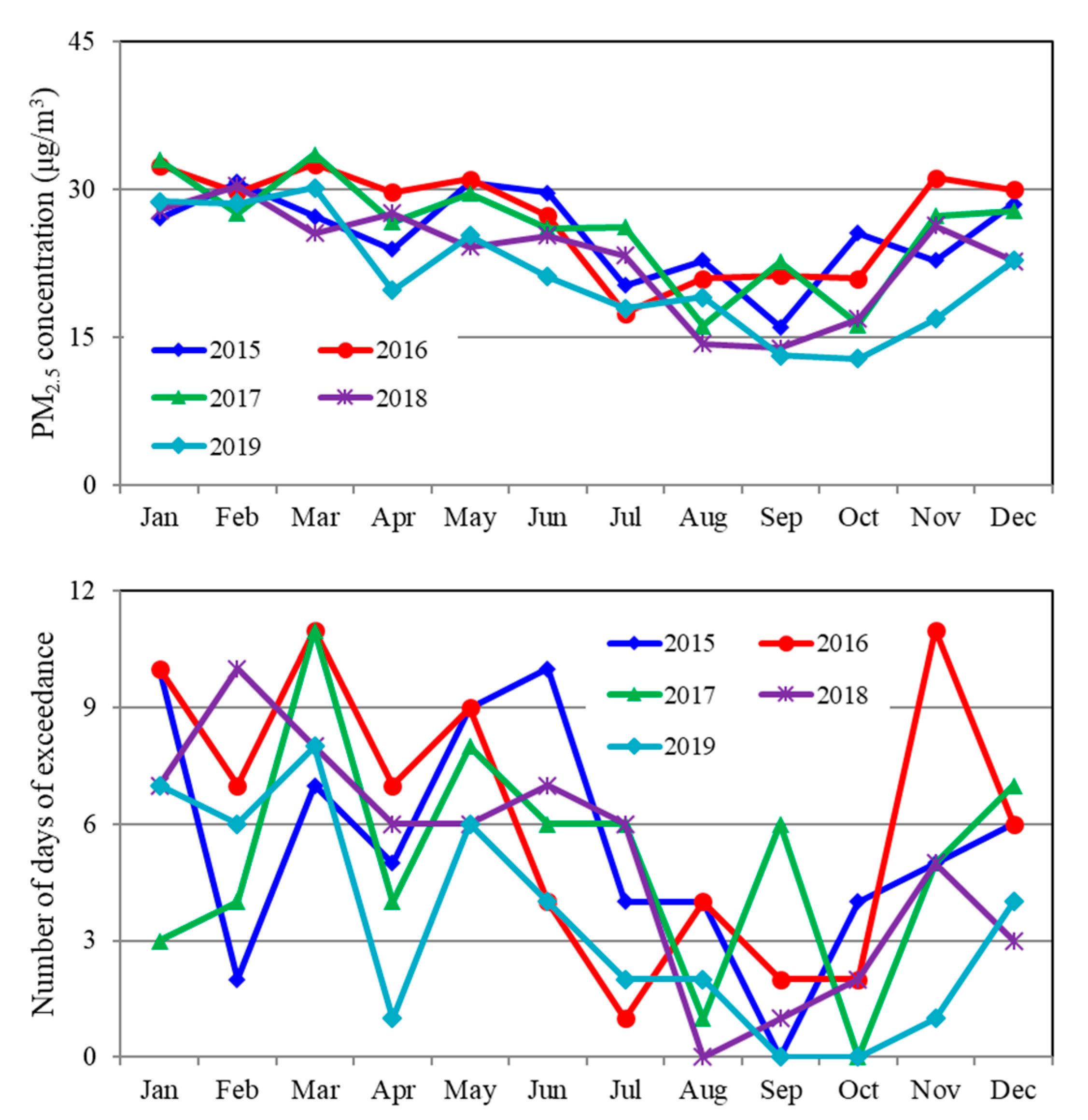
Figure 1. Model domain and grid configuration of the global to mesoscale air quality forecast and analysis system (GMAF).
Atmosphere 12 00411 g001
Figure 2. Schematic diagram of the GMAF.
Atmosphere 12 00411 g002
Figure 3. Four major cities selected for forecast performance evaluation.
Atmosphere 12 00411 g003
Figure 4. Monthly mean PM2.5 concentrations (top) and the number of days exceeding 35 μg/m3 of PM2.5 (bottom) obtained from the Korea air monitoring network in Seoul.
Atmosphere 12 00411 g004
Figure 5. Monthly mean PM2.5 concentrations (top) and the number of days exceeding 35 μg/m3 of PM2.5 (bottom) obtained from the Korea air monitoring network in Busan.
Atmosphere 12 00411 g005
Figure 6. Modeled and observed daily precipitation (top) and daily mean PM2.5 concentrations (bottom) at Seoul.
Atmosphere 12 00411 g006
Figure 7. Modeled chemical compositions of secondary organic aerosols (SOAs) in winter (a), spring (b), summer (c), fall (d) in 2016 in Seoul. pcSOA: potential SOA from combustion, SOA_BVOC: SOA from biogenic volatile organic compounds (VOCs), SOA_AVOC: SOA from anthropogenic VOCs, SOA_gly: SOA from glyoxal and methylglyoxal.
Atmosphere 12 00411 g007
Figure 8. Observed and forecasted monthly mean PM2.5 concentrations at Seoul with the pcSOA weighting factors (PWF) of 0, 0.4 and 1.0.
Atmosphere 12 00411 g008
Figure 9. Monthly observed and forecasted organic carbon concentration at the Bulkwang PM supersite.
Atmosphere 12 00411 g009
Figure 10. Modeled chemical compositions of PM2.5 in winter (a), spring (b), summer (c), fall (d) at Seoul in 2016.
Atmosphere 12 00411 g010
Figure 11. Forecasted monthly mean as-is and retained PM2.5 nitrate at Bulkwang PM2.5 supersite in Korea from December 2015 to November 2016.
Atmosphere 12 00411 g011
Figure 12. Comparison of the nitrate observation and the nitrate forecast at the Bulkwang site in Seoul from April to November 2016.
Atmosphere 12 00411 g012
Table 1. Annual mean concentrations and the number of days exceeding 35 μg/m3 of PM2.5 in Seoul and Busan.
ParameterAnnual Mean
Concentrations (μg/m3)
Number of Days
Exceeding the PM2.5 Threshold
YearSeoulBusanSeoulBusan
201523264266
201626277574
201725266361
201823236161
201925216441
Table 2. Nudged variable and nudging coefficient.
Nudged Variable Nudging Coefficient
Outer DomainInner Nest
WRFU and V winds5.0 × 10−42.5 × 10⁻⁴
Temperature5.0 × 10−42.5 × 10⁻⁴
Water vapor mixing ratio1.0 × 10−41.0 × 10⁻⁴
CMAQSO2, CO, NO, NO2, isoprene, O3, dust, sea salt3.0 × 10−40
Table 3. Statistical analysis on the model performance in forecasting PM2.5 concentration at four cities (Seoul, Busan, Gwangju, Daegu) in 2016 with the PWF changing from 0 to 1.
Region
Name
Weighting
Factor
Continuous ForecastCategorical Forecast
RNMBNMEPODFARHSS
Seoul0.00.764%22%0.680.300.61
0.20.779%23%0.750.350.61
0.40.7813%25%0.810.380.61
0.70.7819%28%0.830.470.53
1.00.7826%33%0.910.520.49
Busan0.00.79−20%26%0.390.160.47
0.20.81−17%24%0.440.140.52
0.40.81−14%22%0.510.160.58
0.70.82−9%21%0.570.200.60
1.00.83−5%21%0.640.250.63
Gwangju0.00.75−2%25%0.490.260.54
0.20.772%25%0.530.360.51
0.40.786%25%0.660.380.58
0.70.8012%26%0.770.390.62
1.00.8118%29%0.890.440.62
Daegu0.00.77−7%23%0.430.190.51
0.20.78−4%22%0.480.240.53
0.40.78−1%22%0.600.300.59
0.70.794%22%0.690.320.62
1.00.799%24%0.740.410.58
Table 4. Goals and criteria of the R, the normalized mean bias (NMB) and the normalized mean error (NME) for the forecast of daily mean PM2.5 concentrations.
RNMBNME
GoalCriteriaGoalCriteriaGoalCriteria
>0.70>0.40<±10%<±30%<±35%<±50%
R = 1 is perfect correlation
R = 0 is no correlation
NMB < 0 is under-forecast
NMB > 0 is over-forecast
NME = 0 is perfect forecast
Table 5. Contingency table structure.
Event
Forecast
Event Observed
YesNo
YesAB
NoCD
Table 6. Performance evaluation of continuous and categorical forecast at Seoul, Busan, Gwangju, Daegu in 2016. A threshold value for the categorical forecast was set to the daily mean PM2.5 35 μg/m3.
PM2.5,obs #Continuous ForecastN_Day %Categorical Forecast
RNMBNMEPODFARHSS
SeoulWinter26.4 μg/m30.8726%27%171.000.480.58
Spring30.2 μg/m30.783%21%310.900.150.81
Summer23.8 μg/m30.7212%26%120.580.530.44
Fall23.8 μg/m30.7712%25%150.600.500.45
Year26.0 μg/m30.7813%25%750.810.380.61
BusanWinter30.2 μg/m30.86−16%20%220.680.170.68
Spring30.8 μg/m30.72−11%23%250.520.240.51
Summer21.8 μg/m30.81−9%20%90.220.000.34
Fall24.5 μg/m30.79−19%25%140.430.000.56
Year26.8 μg/m30.81−14%22%700.510.160.58
GwangjuWinter25.9 μg/m30.8311%24%220.860.270.72
Spring28.0 μg/m30.70−1%25%210.520.420.43
Summer18.6 μg/m30.6811%27%30.001.00−0.03
Fall21.3 μg/m30.807%23%70.710.440.59
Year23.5 μg/m30.786%25%530.660.380.58
DaeguWinter28.6 μg/m30.82−6%19%250.720.180.68
Spring26.3 μg/m30.772%21%160.690.350.59
Summer20.0 μg/m30.647%27%20.001.00−0.03
Fall23.4 μg/m30.79−5%21%150.400.250.46
Year24.6 μg/m30.78−1%22%580.600.300.59
# observed seasonal or yearly averaged concentration of PM2.5. % number of days exceeding PM2.5 standard of 35 μg/m3.
Table 7. Effect of inclusion of nitrate evaporation loss on the performance of continuous and categorical forecast at Seoul, Busan, Gwangju, Daegu during spring and fall in 2016. A threshold value for the categorical forecast was set to the daily mean PM2.5 35 μg/m3.
Nitrate
Evaporation Loss
Continuous ForecastingCategorical Forecasting
RNMBNMEPODFARHSS
SeoulSpringNot included 0.783%21%0.900.150.81
Included0.760%22%0.680.130.67
FallNot included 0.7712%25%0.600.500.45
Included0.774%23%0.330.500.31
BusanSpringNot included 0.72−11%23%0.520.240.51
Included0.67−13%26%0.520.240.51
FallNot included 0.79−19%25%0.4300.56
Included0.78−22%27%0.500.63
GwangjuSpringNot included 0.70−1%25%0.520.420.43
Included0.64−6%27%0.330.420.31
FallNot included 0.807%23%0.710.440.59
Included0.81−2%22%0.290.330.37
DaeguSpringNot included 0.772%21%0.690.350.59
Included0.72−3%23%0.560.250.58
FallNot included 0.79−5%21%0.40.250.46
Included0.80−10%22%0.400.53
Table 8. Performance comparison of continuous and categorical forecast between the additive bias correction, multiplicative bias correction, Kalman filter bias adjustment at Seoul, Busan, Gwangju, Daegu in 2016.
Continuous ForecastCategorical Forecast
RNMBNMEPODFARHSS
SeoulRaw forecast0.7813%25%0.810.380.61
Additive bias correction0.780%23%0.680.320.59
Multiplicative bias correction0.801%21%0.650.340.57
Kalman filter bias adjustment0.827%21%0.800.370.62
BusanRaw forecast0.81−14%22%0.510.160.58
Additive bias correction0.780%21%0.650.320.58
Multiplicative bias correction0.761%23%0.680.330.59
Kalman filter bias adjustment0.83−7%19%0.620.240.62
GwangjuRaw forecast0.786%25%0.660.380.58
Additive bias correction0.790%25%0.680.290.64
Multiplicative bias correction0.781%25%0.620.390.55
Kalman filter bias adjustment0.833%22%0.750.250.71
DaeguRaw forecast0.78−1%22%0.600.300.59
Additive bias correction0.770%23%0.670.340.59
Multiplicative bias correction0.751%23%0.670.380.57
Kalman filter bias adjustment0.82−1%20%0.700.260.66
Publisher’s Note: MDPI stays neutral with regard to jurisdictional claims in published maps and institutional affiliations.

