
Airborne Testing of 2-μm Pulsed IPDA Lidar for Active Remote Sensing of Atmospheric Carbon Dioxide

 ,
, 
Abstract
:1. Introduction
2. Airborne 2-μm Pulsed IPDA Lidar
2.1. IPDA Lidar Transmitter
2.2. IPDA Lidar Receiver and Data Acquisition
2.3. IPDA Lidar Support Instruments
3. CO2 IPDA Lidar Modeling
3.1. XCO2 Retrieval
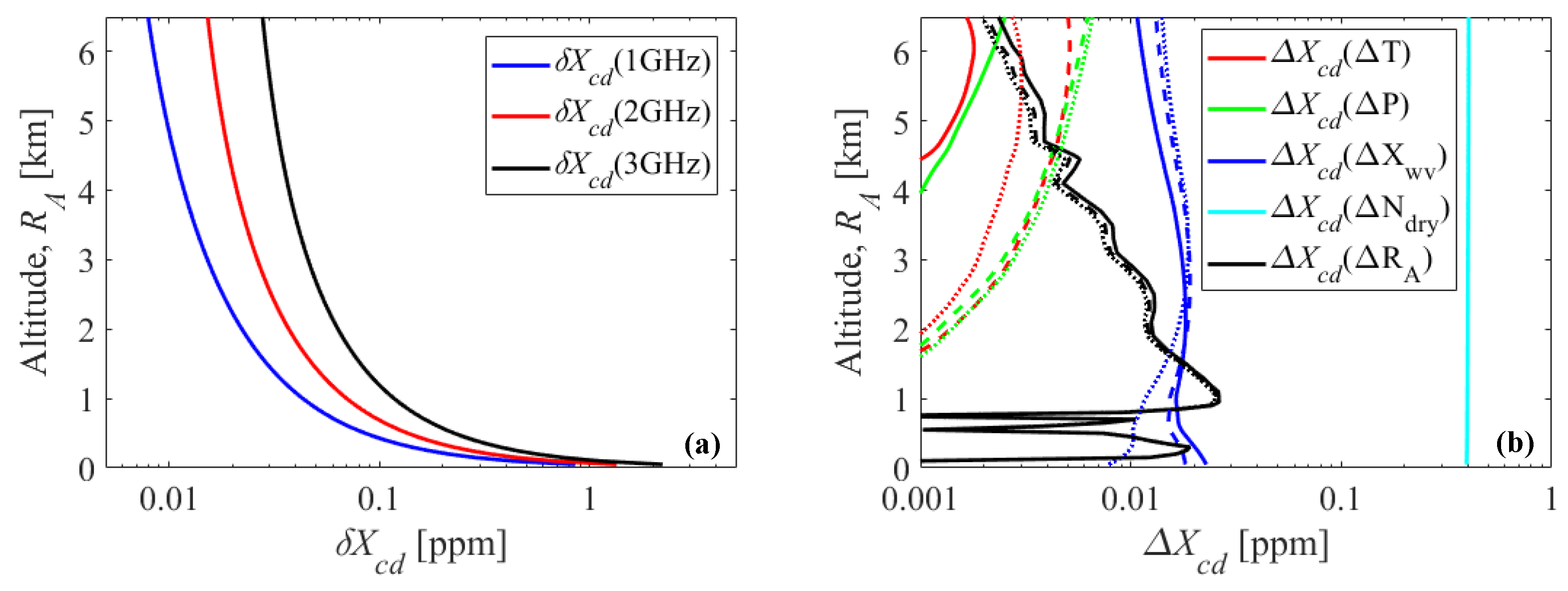
3.2. XCO2 Retrieval Errors
4. IPDA Lidar Measurements
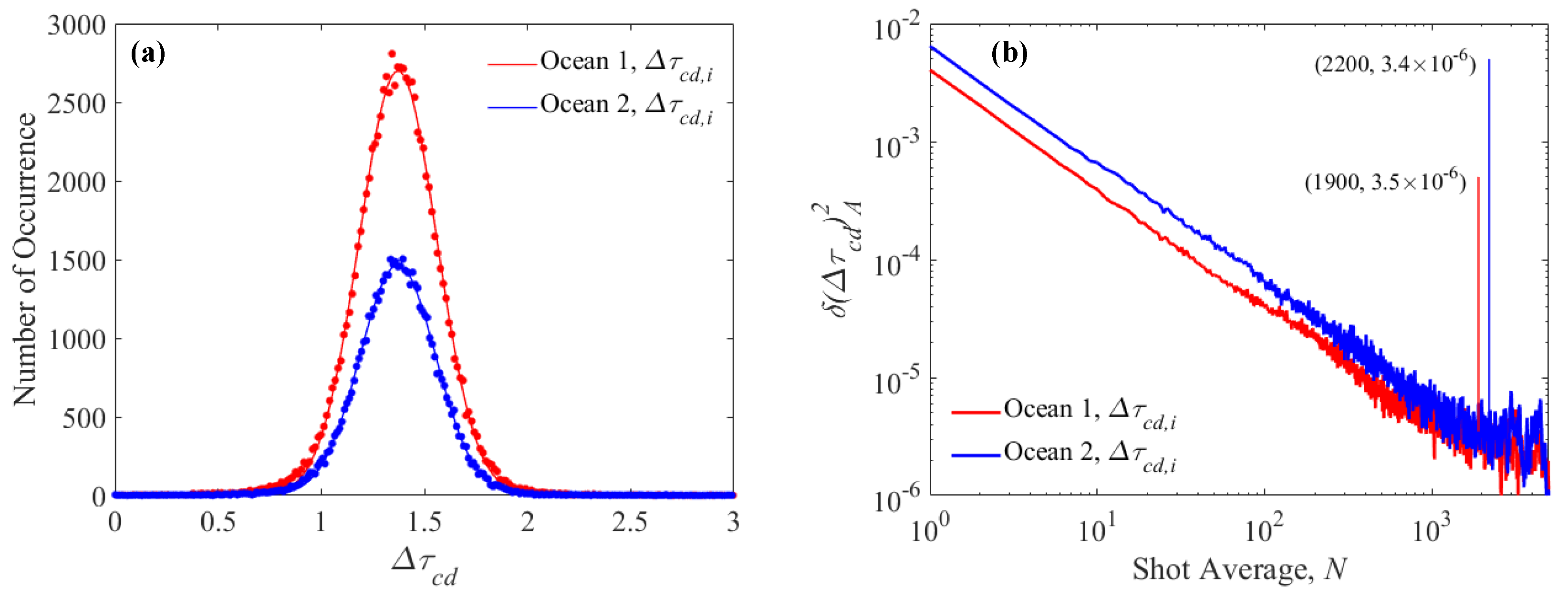
4.1. Ocean Records
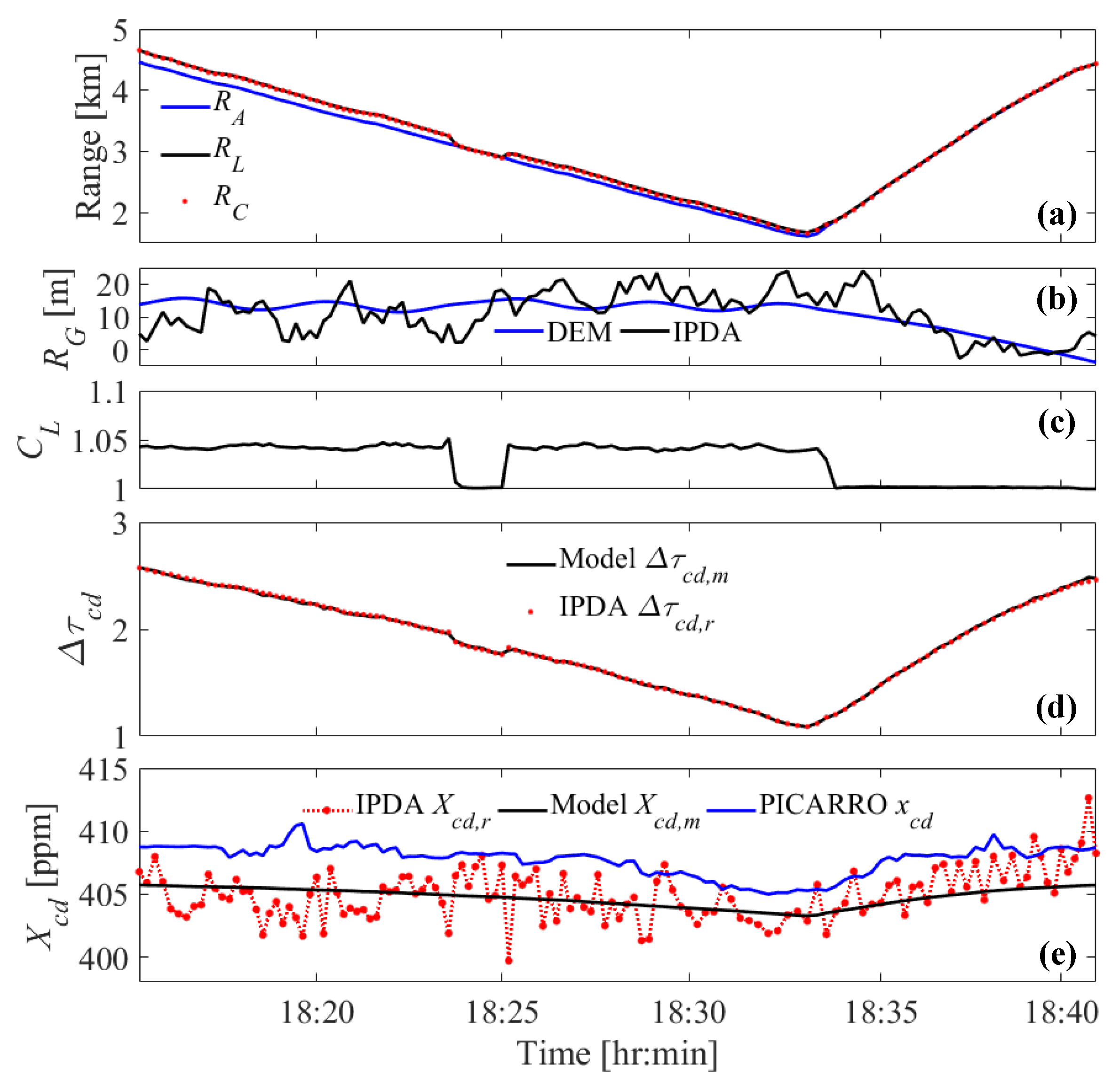
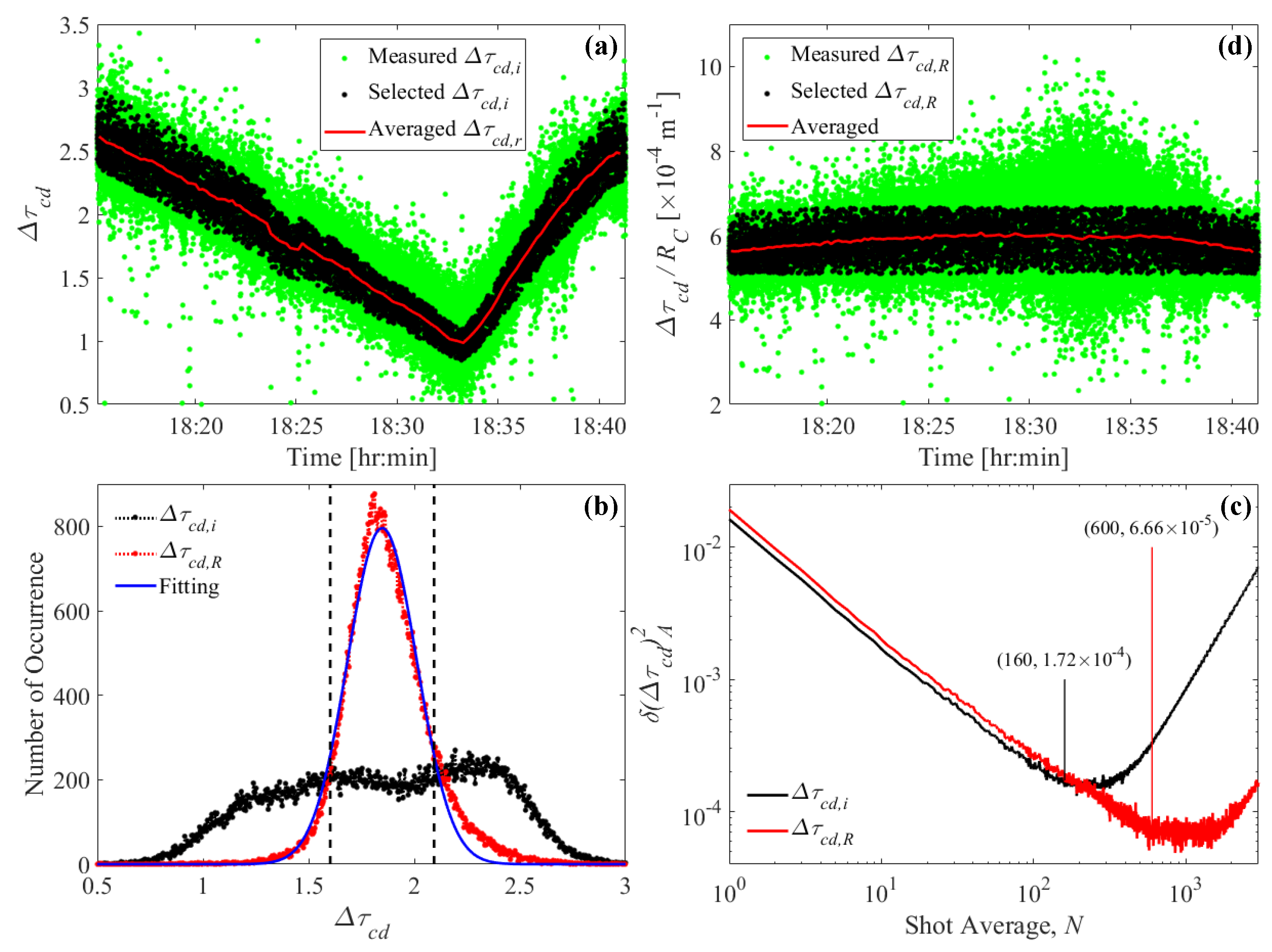
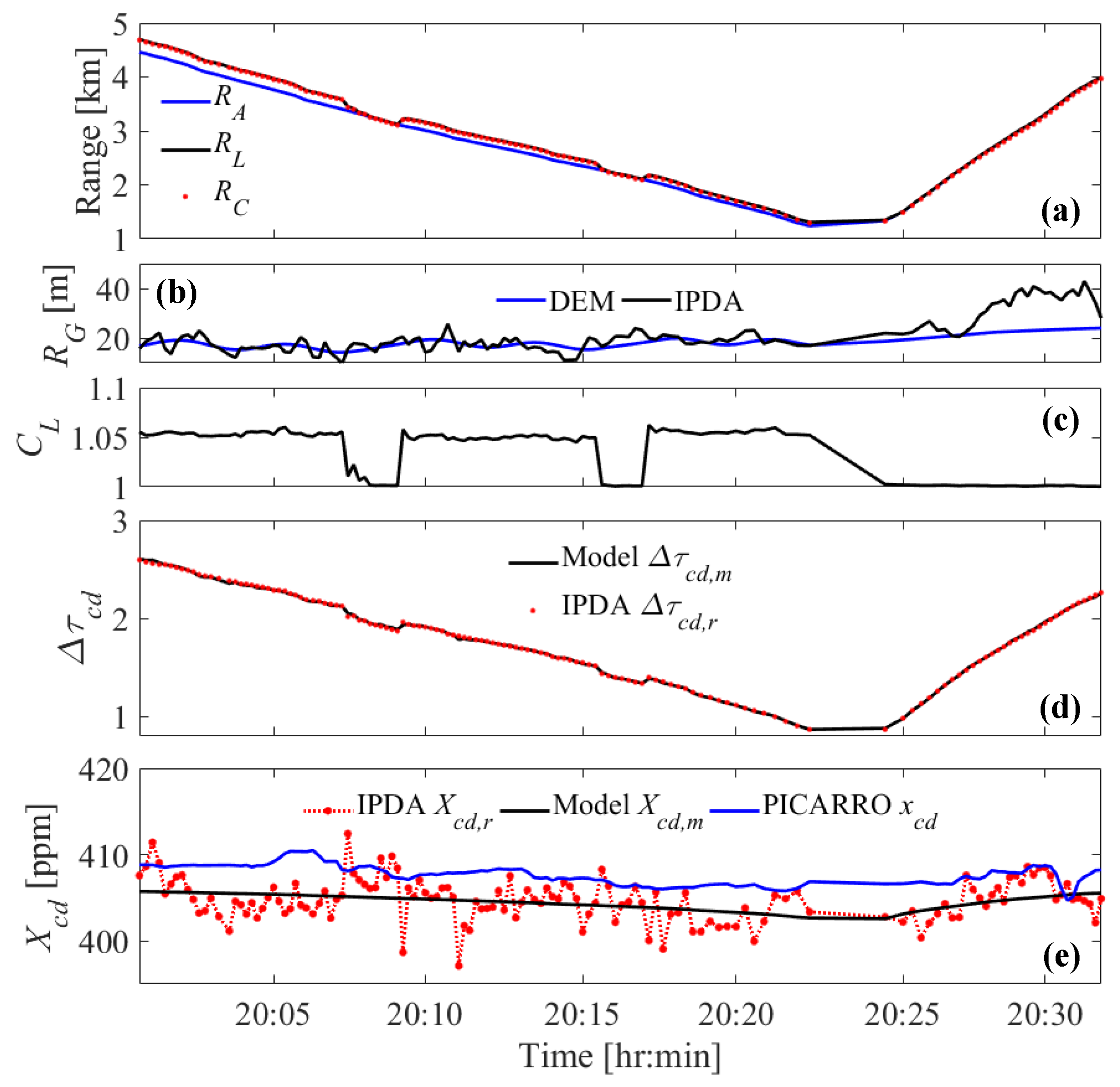
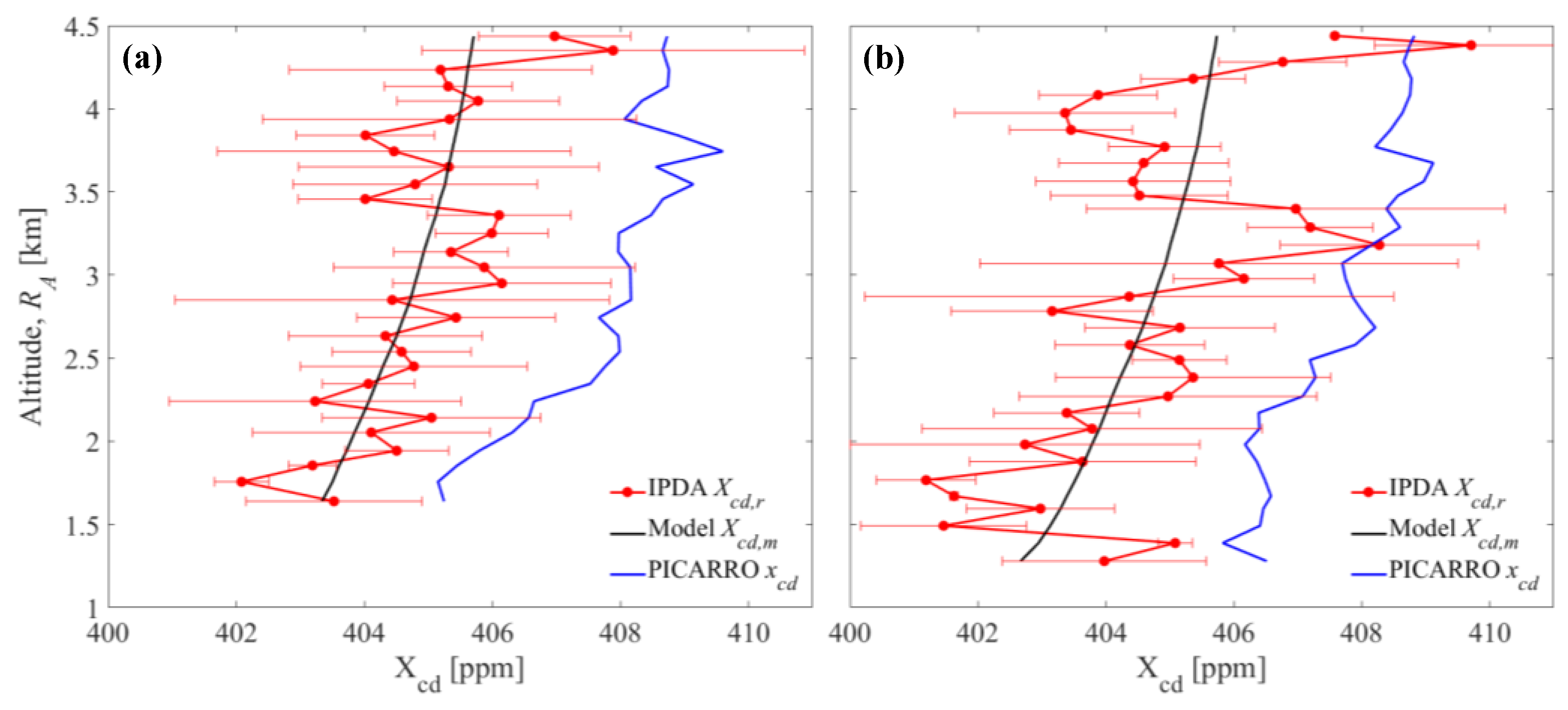
4.2. Spiral Records
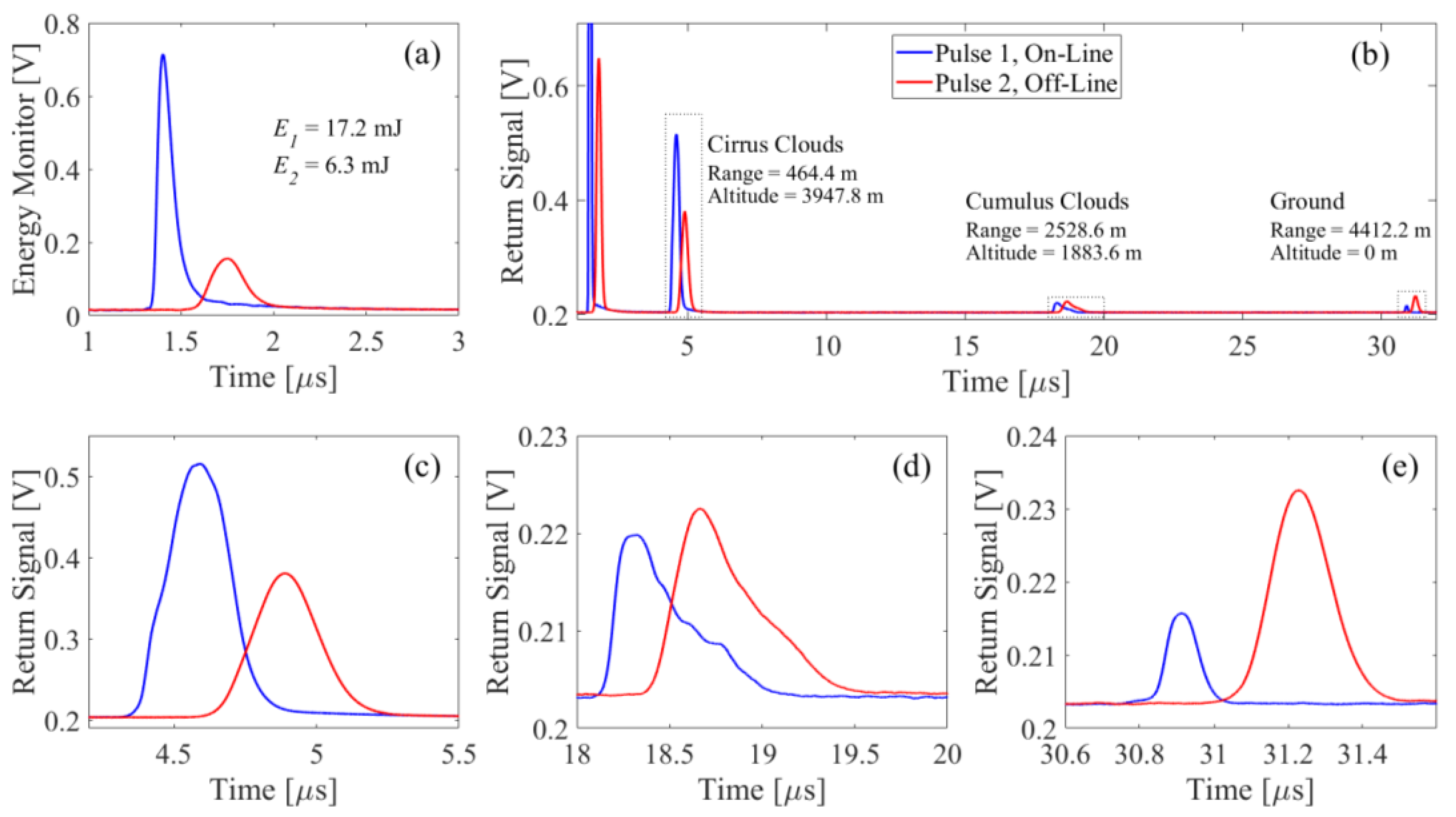
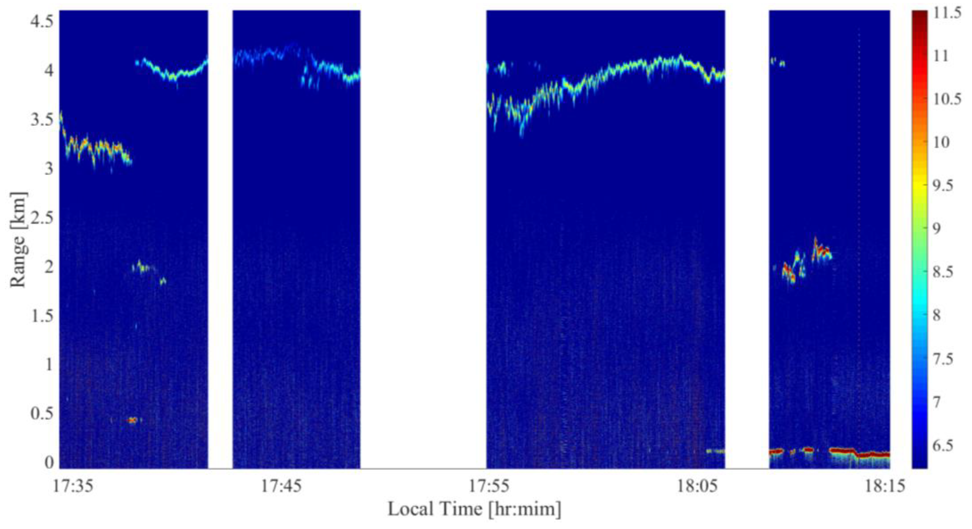
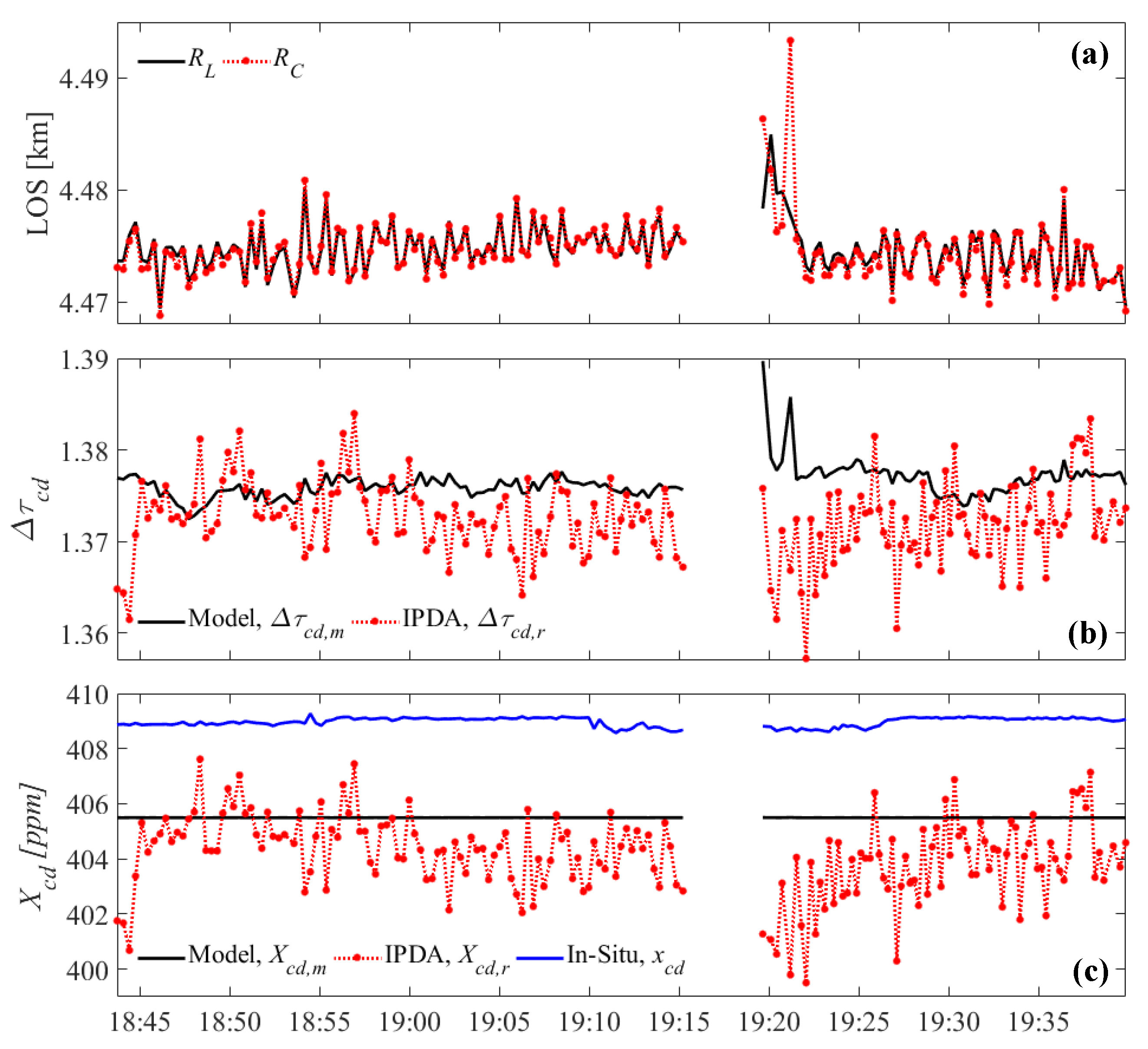
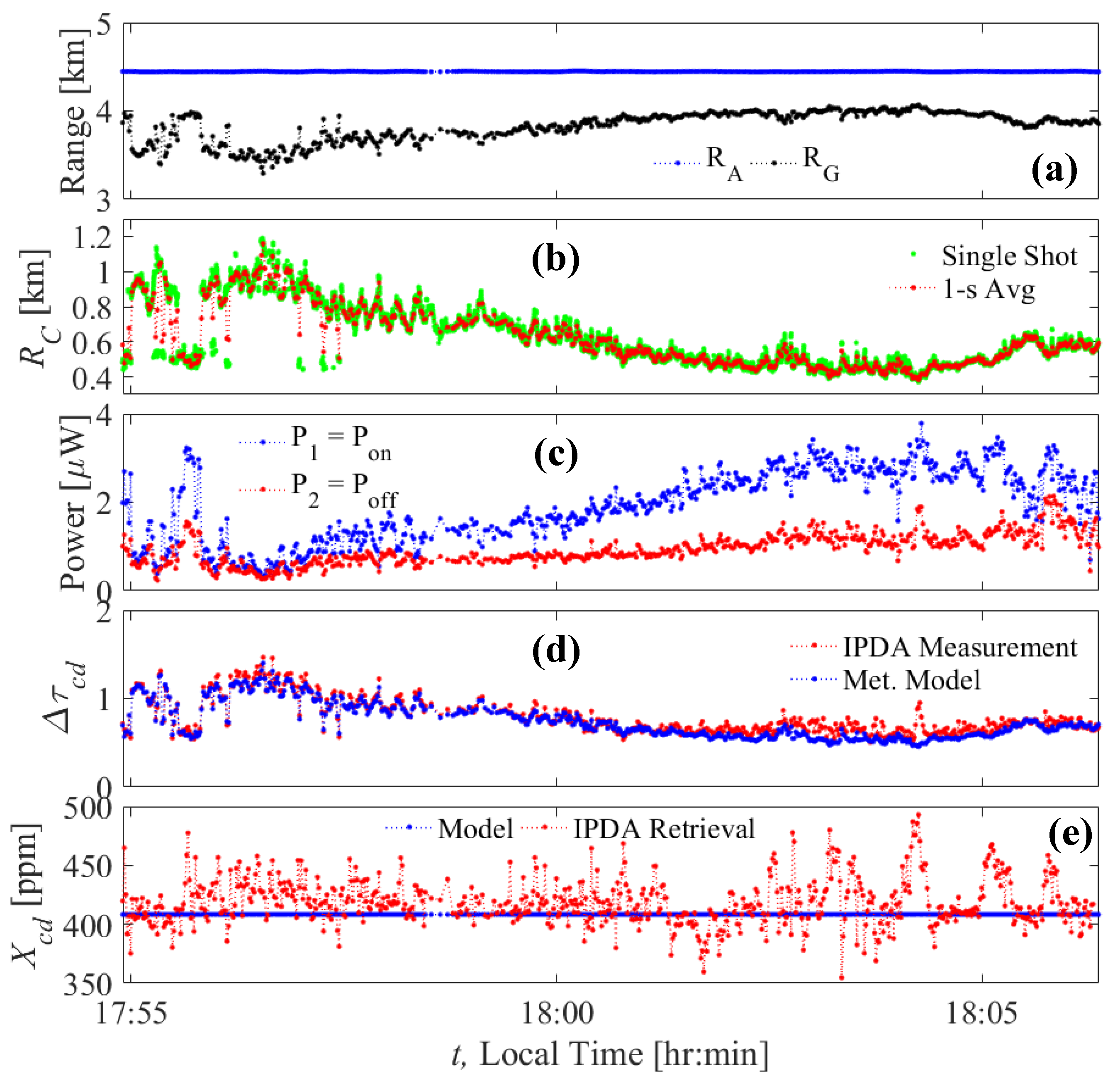
4.3. Clouds Record
5. Conclusions
Author Contributions
Funding
Conflicts of Interest
References
- National Academies of Sciences, Engineering, and Medicine. Thriving on Our Changing Planet: A Decadal Strategy for Earth Observation from Space; The National Academies Press: Washington, DC, USA, 2018. [Google Scholar]
- Wunch, D.; Toon, G.; Blavier, J.; Washenfelder, R.; Notholt, J.; Connor, B.; Griffith, D.; Sherlock, V.; Wennberg, P. The total carbon column observing network. Philos. Trans. R. Soc. A 2011, 369, 2087–2112. [Google Scholar] [CrossRef] [Green Version]
- Sweeney, C.; Karion, A.; Wolter, S.; Newberger, T.; Guenther, D.; Higgs, J.; Andrews, A.; Lang, P.; Neff, D.; Dlugokencky, E.; et al. Seasonal climatology of CO2 across North America from aircraft measurements in the NOAA/ESRL global greenhouse gas reference network. J. Geophys. Res. 2015, 120, 5155–5190. [Google Scholar] [CrossRef]
- Wunch, D.; Wennberg, P.O.; Osterman, G.; Fisher, B.; Naylor, B.; Roehl, C.M.; O’Dell, C.; Mandrake, L.; Viatte, C.; Kiel, M.; et al. Comparisons of the Orbiting Carbon Observatory-2 (OCO-2) XCO2 measurements with TCCON. Atmos. Meas. Tech. 2017, 10, 2209–2238. [Google Scholar] [CrossRef] [Green Version]
- Eldering, A.; Taylor, T.; O’Dell, C.; Pavlick, R. The OCO-3 mission: Measurement objectives and expected performance based on 1 year of simulated data. Atmos. Meas. Technol. 2019, 12, 2341–2370. [Google Scholar] [CrossRef] [Green Version]
- Singh, U.; Refaat, T.; Ismail, S.; Davis, K.; Kawa, S.; Menzies, R.; Petros, M. Feasibility study of a space-based high pulse energy 2 μm CO2 IPDA lidar. Appl. Opt. 2017, 56, 6531–6547. [Google Scholar] [CrossRef]
- Kawa, S.; Abshire, J.; Baker, D.; Browell, E.; Crisp, D.; Crowell, S.; Hyon, J.; Jacob, J.; Jucks, K.; Lin, B.; et al. Active sensing of CO2 emissions over nights, days, and seasons (ASCENDS): Final Report of the ASCENDS Ad Hoc Science Definition Team. NASA/TP 2018, 219034. [Google Scholar]
- Refaat, T.; Petros, M.; Singh, U.; Antill, C.; Remus, R. High-precision and high accuracy column dry-air mixing ratio measurement of carbon dioxide using pulsed 2-μm IPDA lidar. IEEE Trans. Geosci. Remote Sens. 2020, 58, 5804–5819. [Google Scholar] [CrossRef]
- National Research Council. National Imperatives for the Next Decade and Beyond Committee on Earth Science and Applications from Space: A Community Assessment and Strategy for the Future; National Academies: Washington, DC, USA, 2007. [Google Scholar]
- Singh, U.; Walsh, B.; Yu, J.; Petros, M.; Kavaya, M.; Refaat, T.; Barnes, N. Twenty years of Tm:Ho:YLF and LuLif laser development for global wind and carbon dioxide active remote sensing. Opt. Mater. Express 2015, 5, 827–837. [Google Scholar] [CrossRef]
- Refaat, T.; Ismail, S.; Koch, G.; Rubio, M.; Mack, T.; Notari, A.; Collins, J.; Lewis, J.; De Young, R.; Choi, Y.; et al. Backscatter 2-μm lidar validation for atmospheric CO2 differential absorption lidar applications. Trans. Geosci. Remote Sens. 2011, 49, 572–580. [Google Scholar] [CrossRef]
- Refaat, T.; Ismail, S.; Abedin, N.; Spuler, S.; Mayor, S.; Singh, U. Lidar backscatter signal recovery from phototransistor systematic effect by deconvolution. Appl. Opt. 2008, 47, 5281–5295. [Google Scholar] [CrossRef]
- Refaat, T.; Ismail, S.; Koch, G.; Diaz, L.; Davis, K.; Rubio, M.; Abedin, N.; Singh, U. Field-testing of a two-micron DIAL system for profiling atmospheric carbon dioxide. In Proceedings of the 25th International Laser Radar Conference, St. Petersburg, Russia, 5–9 July 2010; pp. 866–869. [Google Scholar]
- Yu, J.; Petros, M.; Singh, U.; Refaat, T.; Reithmaier, K.; Remus, R.; Johnson, W. An airborne 2-μm double-pulsed direct-detection lidar instrument for atmospheric CO2 column measurements. J. Atmos. Ocean. Technol. 2017, 34, 385–400. [Google Scholar] [CrossRef]
- Refaat, T.; Singh, U.; Petros, M.; Remus, R.; Yu, J. Self-calibration and laser energy monitor validations for a double-pulsed 2-μm CO2 integrated path differential absorption lidar application. Appl. Opt. 2015, 54, 7240–7251. [Google Scholar] [CrossRef]
- Refaat, T.; Singh, U.; Yu, J.; Petros, M.; Remus, R.; Ismail, S. Double-pulse 2-μm integrated path differential absorption lidar airborne validation for atmospheric carbon dioxide measurement. Appl. Opt. 2016, 55, 4232–4246. [Google Scholar] [CrossRef] [PubMed]
- Refaat, T.; Singh, U.; Yu, J.; Petros, M.; Remus, R.; Ismail, S. Airborne two-micron double-pulse IPDA lidar validation for carbon dioxide measurements over land. In Proceedings of the 28th International Laser Radar Conference, Bucharest, Romania, 25–30 June 2017; p. 5001. [Google Scholar]
- Refaat, T.; Singh, U.; Yu, J.; Petros, M.; Ismail, S.; Kavaya, M.; Davis, K. Evaluation of an airborne triple-pulsed 2 μm IPDA lidar for simultaneous and independent atmospheric water vapor and carbon dioxide measurements. Appl. Opt. 2015, 54, 1387–1398. [Google Scholar] [CrossRef] [PubMed]
- Petros, M.; Singh, U.; Yu, J.; Refaat, T. Development of double-pulsed two-micron laser for atmospheric carbon dioxide measurements. In Proceedings of the Conference on Lasers and Electro-Optics, San Jose, CA, USA, 14–19 May 2017. JTh2A.8. [Google Scholar]
- Petros, M.; Refaat, T.; Singh, U.; Antill, C.; Remus, R.; Wong, T.; Lee, J.; Ismail, S. Frequency control of multi-pulse 2-micron laser transmitter for atmospheric carbon dioxide measurement. In Proceedings of the IGARSS 2019 IEEE International Geoscience and Remote Sensing Symposium, Piscataway, NJ, USA, 28 July–2 August 2019; pp. 4857–4860. [Google Scholar]
- Refaat, T.; Petros, M.; Singh, U.; Antill, C.; Wong, T.; Remus, R.; Reithmaier, K.; Lee, J.; Bowen, S.; Taylor, B.; et al. Airborne, direct-detection, 2-μm triple-pulse IPDA lidar for simultaneous and independent atmospheric water vapor and carbon dioxide active remote sensing. Proc. SPIE 2018, 10779, 1077902. [Google Scholar]
- Refaat, T.; Petros, M.; Remus, R.; Singh, U. MCT APD detection system for atmospheric profiling applications using two-micron lidar. EPJ Web Conf. 2020, 237, 01013. [Google Scholar] [CrossRef]
- Bagheri, M.; Spiers, G.; Frez, C.; Forouhar, S. Line width Measurement of distributed-feedback semiconductor Lasers operating near 2.05-μm. IEEE Photon. Technol. Lett. 2015, 27, 1934–1937. [Google Scholar] [CrossRef]
- Gordon, I.E.; Rothman, L.S.; Hill, C.; Kochanov, R.V.; Tan, Y.; Bernath, P.F.; Birk, M.; Boudon, V.; Campargue, A.; Chance, K.V.; et al. The HITRAN2016 molecular spectroscopic database. J. Quant. Spectrosc. Radiat. Transf. 2017, 203, 3–69. [Google Scholar] [CrossRef]
- Rothman, L.S.; Rinsland, C.P.; Goldman, A.; Massie, S.T.; Edwards, D.P.; Flaud, J.M.; Perrin, A.; Camy-Peyret, C.; Dana, V.; Mandin, J.Y.; et al. The HITRAN molecular spectroscopic database and HAWAKS (HITRAN atmospheric workstation): 1996 edition. J. Quant. Spectrosc. Radiat. Transf. 1998, 60, 665–710. [Google Scholar] [CrossRef]
- Refaat, T.; Petros, M.; Lee, J.; Wong, T.; Remus, R.; Singh, U. Laser energy monitor for triple-pulse 2-μm IPDA lidar application. Proc. SPIE 2018, 10779, 1077905. [Google Scholar]
- Menzies, R. Coherent and incoherent Lidar—An overview. In Tunable Solid State Lasers for Remote Sensing; Springer: Berlin, Germany, 1985; pp. 17–21. [Google Scholar]
- Casse, V.; Gibert, F.; Edouart, D.; Chomette, O.; Crevoisier, C. Optical energy variability induced by speckle: The cases of MERLIN and CHARM-F IPDA lidar. Atmosphere 2019, 10, 540. [Google Scholar] [CrossRef] [Green Version]
- Sun, X.; Abshire, J.; Krainak, M.; Lu, W.; Beck, J.; Sullivan, W.; Mitra, P.; Rawlings, D.; Fields, R.; Hinkley, D.; et al. HgCdTe avalanche photodiode array detectors with single photon sensitivity and integrated detector cooler assemblies for space lidar applications. Opt. Eng. 2019, 58, 067103. [Google Scholar]
- Sun, X.; Abshire, J.; Beck, J.; Mitra, P.; Reiff, K.; Yang, G. HgCdTe avalanche photodiode detectors for airborne and space borne lidar at infrared wavelengths. Opt. Exp. 2017, 25, 16589–16602. [Google Scholar] [CrossRef] [PubMed]
- Refaat, T.; Singh, U.; Petros, M.; Remus, R. MCT avalanche photodiode detector for two-micron active remote sensing applications. In Proceedings of the IEEE International Geoscience and Remote Sensing Symposium, Valencia, Spain, 22–27 July 2018; pp. 1865–1868. [Google Scholar]
- Anderson, G.; Clough, S.; Kneizys, F.; Chetwynd, J.; Shettle, E. AFGL atmospheric constituent profiles (0–120 km). In Environmental Research Papers; AFGL-TR-86-0110 No. 954; Air Force Geophysics Laboratory: Hanscom AFB, MA, USA, 1986. [Google Scholar]
- Ehret, G.; Kiemle, C.; Wirth, M.; Amediek, A.; Fix, A.; Houweling, S. Space-borne remote sensing of CO2, CH4 and N2O by integrated path differential absorption Lidar: A sensitivity analysis. Appl. Phys. B 2008, 90, 593–608. [Google Scholar] [CrossRef] [Green Version]


| Transmitter | |
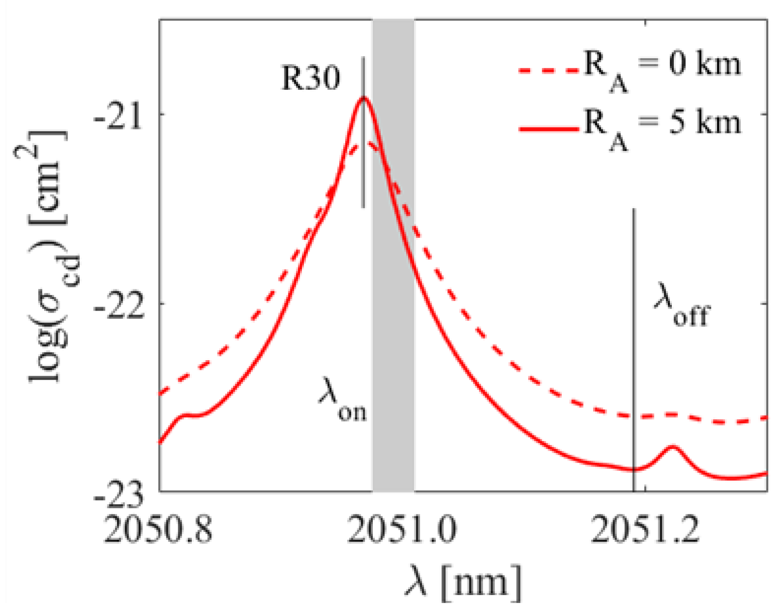
| Off-Line Wavelength | 2051.1905 nm (15.93 GHz) |
| On-Line Wavelength (Tunable) | 2050.875–2051.010 nm (0.5–3.0 GHz) |
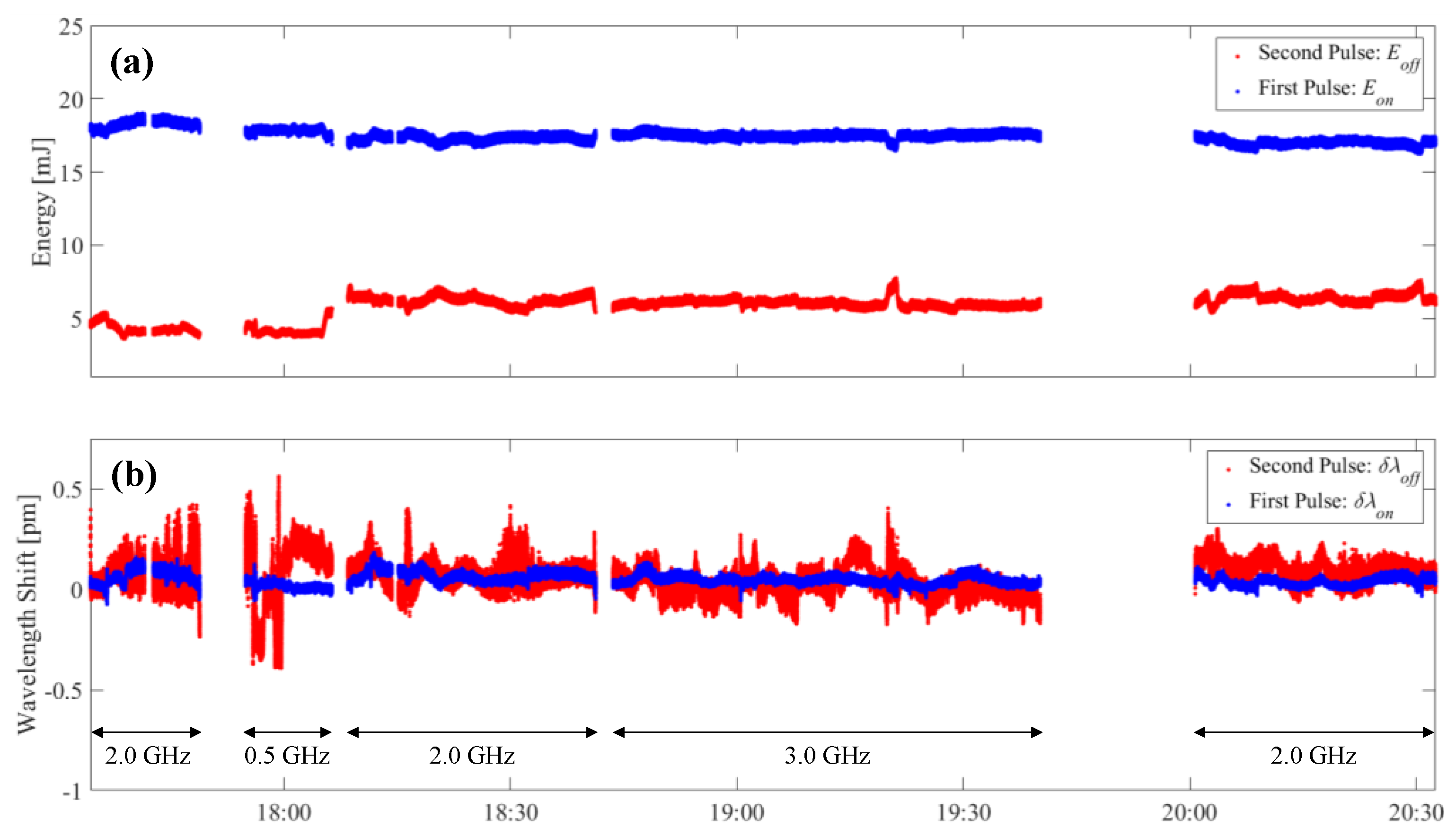
| Pulse Energy (On/Off) | 17.5/6 mJ |
| Beam Divergence | 180 μrad |
| Beam Diameter | 16 mm |
| Electrical-to-optical Efficiency | 1.0% |
| Receiver | |
| Telescope Diameter | 0.4 m |
| Field-of-View | 350 μrad |
| Optical Efficiency | 65% |
| Low-Signal (10%) Channel using PIN Detection System | |
| Detector Type | InGaAs pin photodiode |
| Detector Responsivity | 1.15 A/W |
| Detector Diameter | 300 μm |
| TIA Gain, Bandwidth, NEP | 104 V/A, 10 MHz, 55 pW/Hz1/2 |
| High-Signal (90%) Channel using e-APD Detection System | |
| Detector Type | HgCdTe e-APD |
| Detector Responsivity | 1.05 A/W |
| Detector Size | 80 × 80 μm2 pixel (4 × 4 pixels) |
| Avalanche and TIA Total Gain | 1.1 × 10⁸ V/W at 12 V and 77 K |
| Bandwidth, NEP | 6 MHz, 9.2 fW/Hz1/2 |
| Ocean 1 | Ocean 2 | Spiral 1 | Spiral 2 | Cloud | |
|---|---|---|---|---|---|
| Total Shots | 106,450 | 63,000 | 78,450 | 94,700 | 32,200 |
| λon (GHz) | 3.0 | 3.0 | 2.0 | 2.0 | 0.5 |
| VB (V) | 8.0 | 8.0 | 5.0 | 5.5 | 3.0 |
| Eon (mJ) | 17.49 ± 0.11 | 17.49 ± 0.14 | 17.30 ± 0.17 | 16.99 ± 0.18 | 17.77 ± 0.14 |
| Eoff (mJ) | 6.01 ± 0.13 | 5.83 ± 0.26 | 6.11 ± 0.30 | 6.37 ± 0.28 | 4.13 ± 0.42 |
| Pon (μW) | 0.14 ± 0.05 | 0.22 ± 0.05 | 0.50 ± 0.20 | 0.50 ± 0.30 | 1.90 ± 0.80 |
| Poff (μW) | 0.19 ± 0.06 | 0.29 ± 0.06 | 0.90 ± 0.50 | 1.00 ± 0.50 | 9.40 ± 0.30 |
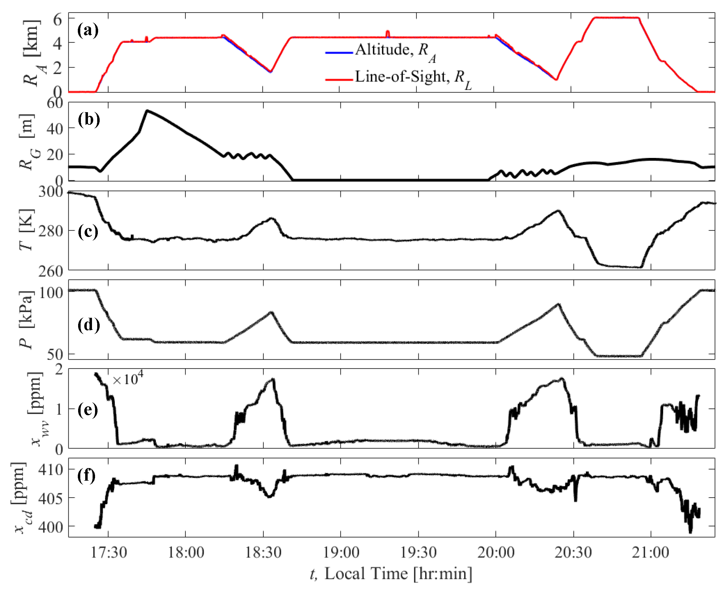
| RA (m) | 4474.3 | 4474.8 | 4464.2 1610.7 | 4458.1 1240.1 | 4446.6 |
| RC ± δRC (m) | 4474.8 ± 2.0 | 4474.2 ± 3.4 | 4644.3 ± 9.5 1653.3 ± 5.3 | 4684.3 ± 20 1292.3 ± 18 | 620.9 ± 167.4 |
| Xcd,m ± δXcd,m (ppm) | 405.49 ± 0.01 | 405.49 ± 0.02 | 404.75 ± 0.73 | 404.58 ± 0.90 | 408.26 ± 0.20 |
| Xcd,r ± δXcd,r (ppm) | 404.43 ± 1.23 | 403.76 ± 1.58 | 404.89 ± 1.19 | 404.71 ± 1.91 | 418.97 ± 20.0 |
| ΔXcd (ppm) | 1.07 | 1.73 | 0.15 | 0.13 | 10.71 |
| δXcd (ppm) | 1.23 | 1.58 | 0.94 | 1.68 | 20.02 |
| εS (%) | 0.26 | 0.43 | 0.04 | 0.03 | 2.56 |
| εR (%) | 0.30 | 0.39 | 0.23 | 0.42 | 4.78 |
Publisher’s Note: MDPI stays neutral with regard to jurisdictional claims in published maps and institutional affiliations. |
© 2021 by the authors. Licensee MDPI, Basel, Switzerland. This article is an open access article distributed under the terms and conditions of the Creative Commons Attribution (CC BY) license (http://creativecommons.org/licenses/by/4.0/).
Share and Cite
Refaat, T.F.; Petros, M.; Antill, C.W.; Singh, U.N.; Choi, Y.; Plant, J.V.; Digangi, J.P.; Noe, A. Airborne Testing of 2-μm Pulsed IPDA Lidar for Active Remote Sensing of Atmospheric Carbon Dioxide. Atmosphere 2021, 12, 412. https://doi.org/10.3390/atmos12030412
Refaat TF, Petros M, Antill CW, Singh UN, Choi Y, Plant JV, Digangi JP, Noe A. Airborne Testing of 2-μm Pulsed IPDA Lidar for Active Remote Sensing of Atmospheric Carbon Dioxide. Atmosphere. 2021; 12(3):412. https://doi.org/10.3390/atmos12030412
Chicago/Turabian StyleRefaat, Tamer F., Mulugeta Petros, Charles W. Antill, Upendra N. Singh, Yonghoon Choi, James V. Plant, Joshua P. Digangi, and Anna Noe. 2021. "Airborne Testing of 2-μm Pulsed IPDA Lidar for Active Remote Sensing of Atmospheric Carbon Dioxide" Atmosphere 12, no. 3: 412. https://doi.org/10.3390/atmos12030412