Article

Long-Term Study on Medium-Scale Traveling Ionospheric Disturbances Observed over the South American Equatorial Region

by
Patrick Essien
1,2,3,*,
Cosme Alexandre Oliveira Barros Figueiredo
1,
Hisao Takahashi
1,
Cristiano Max Wrasse
1,
Diego Barros
1,
Nana Ama Browne Klutse
2,3,4,
Solomon Otoo Lomotey
1,
Toyese Tunde Ayorinde
1,
Delano Gobbi
1 and
Anderson V. Bilibio
1
1
National Institute for Space Research (INPE), Division of Aeronomy Av. dos Astronautas, Sao Jose dos Campos CEP 12227-010, SP, Brazil
2
Climate Change and Atmospheric Physics Center, African Institute for Mathematical Sciences (AIMS) Ghana, Accra P.O. Box LG DTD 20046, Ghana
3
African Institute of Mathematical Sciences (AIMS), Sector Remera, Kigali 20093, Rwanda
4
Department of Physics, University of Ghana, Accra P.O. Box LG 63, Ghana
*
Author to whom correspondence should be addressed.
Atmosphere 2021, 12(11), 1409; https://doi.org/10.3390/atmos12111409
Submission received: 9 September 2021 / Revised: 13 October 2021 / Accepted: 20 October 2021 / Published: 26 October 2021
(This article belongs to the Special Issue Ionospheric Monitoring and Modelling for Space Weather)

Abstract

:
Using data collected by the GNSS dual-frequency receivers network, de-trended TEC maps were generated to identify and characterize the medium-scale traveling ionospheric disturbances (MSTIDs) over the South American equatorial region (latitude: 0 to 15 S and longitude: 30 to 55 W) during solar cycle 24 (from January 2014 to December 2019). A total of 712 MSTIDs were observed during quiet geomagnetic conditions. The Frequency of occurrence of MSTID is high during the solar maximum and low in the minimum phase. This might be due to the solar cycle dependence of gravity wave activity in the lower atmosphere and gravity wave propagation conditions in the thermosphere. The predominant daytime MSTIDs, representing 80% of the total observations, occurred in winter (June-August season in the southern hemisphere) with the secondary peak in the equinox; while the evening time MSTIDs, representing 18% of the entire events, occurred in summer (December to February season) and equinox (March to May and September to November), and the remaining 2% of the MSTIDs were observed during nighttime. The seasonal variation of the MSTID events was attributed to the source mechanisms generating them, the wind filtering and dissipation effects, and the local time dependency. The horizontal wavelengths of the MSTIDs were mostly concentrated between 500 and 800 km, with the mean value of 667 ± 131 km. The observed periods ranged from 30 to 45 min with the mean value of 36 ± 7 min. The observed horizontal phase speeds were distributed around 200 to 400 m/s, with the corresponding mean of 301 ± 75 m/s. The MSTIDs in the winter solstice and equinoctial months preferentially propagated northeastward and northwestward. Meanwhile, during the summer solstice, they propagated in all directions. The anisotropy of the propagation direction might be due to several reasons: the wind and dissipative filtering effects, ion drag effects, the primary source region, and the presence of the secondary or tertiary gravity waves in the thermosphere. Atmospheric gravity waves from strong convective sources might be the primary precursor for the observed equatorial MSTIDs. In all seasons, we noted that the MSTIDs propagating southeastward were probably excited by the likely gravity waves generated by the intertropical convergence zone (ITCZ).

1. Introduction

The existence of disturbances in the ionosphere is very crucial to the electrodynamics of the equatorial ionosphere. Among others, medium-scale traveling ionospheric disturbances (MSTIDs) are known to be the plasma density fluctuations that propagate as waves through the ionosphere at a wide range of velocities and frequencies [1,2,3]. These wave-like perturbations of the ionospheric plasma have horizontal phase velocities of hundreds of meters per second (m/s), periods of less than 1 h, and wavelengths of several hundred to a few thousand kilometers [4,5,6]. They vary with latitude, longitude, local time, season, and solar activities [3,7,8]. They were first postulated to be the ionospheric manifestation of gravity waves from the neutral atmosphere by [9]. However, the advent of two-dimension Global Navigation Satellite System (GNSS) receivers and all-sky imagers, ionosondes, incoherent scatter radars, and HF Doppler systems and models, among others, have revealed that MSTIDs are generated by different mechanisms between daytime and nighttime [10,11,12], due to the variation in their propagation direction between daytime and nighttime. Thus, in midlatitudes, the Perkins instabilities [13] are considered to be the precursor of the nighttime MSTIDs. The interlink between the E region and F region, with regard to MSTID propagation direction, has also been reported by [14].
MSTIDs constitute a specific type of space weather and geophysical phenomenon that can be solar-driven or driven by other processes from auroral sources at the high latitude thermosphere to the solar terminator and storms, tropospheric convection, hurricanes, and tornadoes in the troposphere [11,15]. Independently of the MSTIDs sources, the effects introduce irregularities in the ionospheric plasma that provoke and eventually affect the radio wave propagations. The main concern of the scientific community is to be able to have direct and timely information of MSTID events and hence, are able to mitigate the effects in the affected operations. Meanwhile, due to the high occurrence rate of MSTIDs on a daily basis, and the variety of their characteristics regarding the velocity, wavelength, period, propagation direction, and amplitude, their identification and tracking are very complicated and have not yet been fully achieved in operational service mode.
The long-term characteristics of MSTIDs in the South American equatorial region are not well known. Meanwhile, there is a need to better understand their morphology and climatology and ultimately predict their behavior more accurately in the future. Before such improvements are achieved, more measurements are needed in all regions. However, there are not enough useful F-region climatology studies on MSTID over the South American equatorial region that could be the fundamental result as far as the subject matter is concerned. Therefore, any operational requirement for MSTID information means that their characteristics have to be known at various locations. Due to the variability of MSTIDs, their occurrence, even on a statistical basis, are unable to be predicted. This variability arises from the multiple sources of gravity waves in both the troposphere and thermosphere and the variability of the medium (background winds and temperature) through which they propagate.
The equatorial ionosphere possesses distinguishing features from the other latitudes due to the low inclination of the geomagnetic field lines and the relatively larger fraction of the incident solar ionizing radiation that characterizes the region. The region in question can be characterized by the highest values of the peak-electron density with the most pronounced amplitude and phase scintillation effects. The combined effects of the higher solar flux entrance, and electric and magnetic fields of the earth result in a rising of the plasma along the magnetic field lines. This leads to a phenomenon known as Equatorial Ionization Anomaly (EIA), when the rising plasma loses its momentum and energy, and the gravity and pressure gradient act upon it. AThe South American equatorial ionosphere is among the regions where high spatial variations of the ionospheric plasma density can be found. There is a particular interest in MSTIDs in this region because of their implied role [10] in triggering plasma bubbles and associated strong Spread F irregularities, which, in turn. can cause dropouts and scintillations of the GNSS-based systems [16]. Some works have already reported that MSTIDs [17,18] are a possible candidate to generate equatorial plasma bubbles or irregularities, especially whenever the Rayleigh–Taylor instability is active [19].
Nighttime MSTIDs have been extensively observed over the low and equatorial latitudes of South America [20,21,22,23,24,25,26], mid-latitude [5,6,27,28] at the atomic oxygen red line airglow emission (OI 630.0 nm) by all-sky-imagers, and equatorial region over Asia [29,30]. Ref. [31] used two-dimensional maps of TEC obtained from a dense GPS-receiver network in Japan to study daytime MSTIDs for the first time. Ref. [11] also studied the local time and seasonal variations of MSTIDs over southern California, while [7] analyzed the GPS-TEC data to show seasonal and local time variations of MSTIDs and later studied the same phenomena over Europe [6]. In China, [32] clarified MSTID statistically. So far, the only study on the daytime MSTID characteristics in the South American equatorial region was conducted by [33], using one-year measurement made at three positions by ionosonde over northeast Brazil. Ref. [12] recently reported the influence of solar activities on the MSTIDs. So far, no detailed statistical analysis has been done on the daytime MSTIDs in the South American equatorial region.
Ref. [34] reported the characteristics of geomagnetic conjugate MSTIDs but was limited to daytime summer MSTIDs that were generated at the conjugate hemispheres. Ref. [35] investigated MSTID characteristics in the low to middle latitude (15–30 S) region of South America during the period 2012–2016. They reported variations in the frequency of occurrence of MSTID, day to night, and seasonally. In our present study, we focus on the latitudinal coverage from the equator to low latitudes (0–15 S) and long-term coverings from the high to low solar activity period (2012–2019) covering solar cycle 24.
For that matter, the overarching objectives of this work were to study the long-term statistical analysis and characteristics of MSTIDs over the South American equatorial region during Solar Cycle 24.

2. Materials and Methods

Approximately 236 dual-frequency GNSS receivers are installed in the South American region. Among them, 83 are located in the equatorial region where the present work was conducted. Figure 1 shows the distribution of the GNSS ground-based receivers network of South America operated by RMBC, RAMSAC, LISN, and IGS (represented in red, blue, violet, and green, respectively) which show their latitudinal and longitudinal positions. The area of the present study is indicated by a red rectangle, covering the latitudes 0 to 15 S and longitudes 30 to 55 west, equivalent to a distance 1667 km by 2778.0 km, respectively, and a total area of 4,630,926 km 2 . This area selected was located mainly below the magnetic equator to investigate the possible source regions of the MSTIDs that propagate over the region. The western part of the continent is above the magnetic equator, as it Amazon Rainforest, which could be investigated in the future.
The carrier phase delays and group delays are the two basic observables that are provided by the dual-frequency GNSS signals in every 30 s for each day. The slant TEC (STEC), which is the line integral of electron density along the signal path between the receiver and a satellite given in the TEC units (1 TECU = 10 16 m 2 ), are expressed by Mannucci et al. [36] as:
T E C = 1 40.3 f i 2 f j 2 ( f i 2 f j 2 ) [ ( L i L j ) ( λ i N i λ j N j ) + b r + b s ]
where L i and L j are the carrier phase signal (converted to distance units). λ i N i and λ j N j are integer cycle ambiguities, and b r and b s are satellite and receiver instrumental biases. The f i and f j correspond to the frequencies of GPS and GLONASS (in the latter, every two satellites have the same dual frequencies). Due to the ambiguity in the carrier phase measurements, the level of the TEC is unknown. Meanwhile, the level is adjusted to the slant TEC derived from the pseudoranges for each satellite-receiver pair. The TEC obtained by the above procedure still contains biases inherent in satellite and receiver hardware. Moreover, the ambiguities, as well as the biases, of both the satellite and receiver ought to be estimated to obtain the absolute value of TEC [5,8]. However, this study is not interested in the absolute TEC, but instead focusing on the perturbation components of TEC caused by MSTIDs.
The Vertical TEC (VTEC) can be obtained by the product of the slant TEC (STEC) and cosine of the zenith angle ( ψ ):
V T E C = T E C × c o s ( ψ )
where the ψ of the signal path through the ionospheric piercing point (IPP) in the F2 region can be estimated as:
ψ = π 2 E l a r c s i n R e / ( R e + 300 ) × c o s ( E l )
where R e is the radius of the Earth, E l is the elevation angle, which can be estimated from the ephemeris file, called Sp3 (Standard parameter 3), that gives the final orbital position (XYZ coordinates) of the satellite for both GPS and GLONASS in every 30 min. In this case, interpolation is necessary to synchronize the time of the XYZ coordinates with that of the TEC. The GPS broadcast ephemeris are linked to the position of the satellite antenna phase center in the World Geodetic Service-84 (WGS-84) reference frame. WGS-84 is a unified terrestrial reference system for the position and vector referencing of GPS. Whereas, GLONASS broadcast ephemeris are given in the Parametry Zemli 1990 (Parameters of the Earth 1990) (PZ-90) reference frame. Therefore, we transformed the XYZ coordinates from PZ-90 to the WGS-84 [37,38,39].
The detrending TEC (dTEC) is calculated by subtracting one hourly moving average ( V T E C ( t ± 30 min) from the corresponding time sequence of VTEC(t) [5,6,8,31,35]:
d T E C ( t ) = V T E C ( t ) < V T E C ( t ± 30 m i n ) >
Figure 2 shows the TEC with its running average (upper panel) and the dTEC (lower panel) GPS PRN 32. TEC values of elevation angles greater than 30 are used in the present work in order to minimize errors due to cycle slips and slant factors [5]. The upper panel shows the VTEC profile (black) and the corresponding one hour running average ( ± 30 min) TEC (red), while the lower panel is the TEC perturbation cause by MSTIDs which can be seen at the amplitude greater than 0.2 TECU [5,6,11,35]. The maximum MSTID oscillations are seen between 9:00 UT and 12:05 UT, and 13:00 and 15:00 UT.

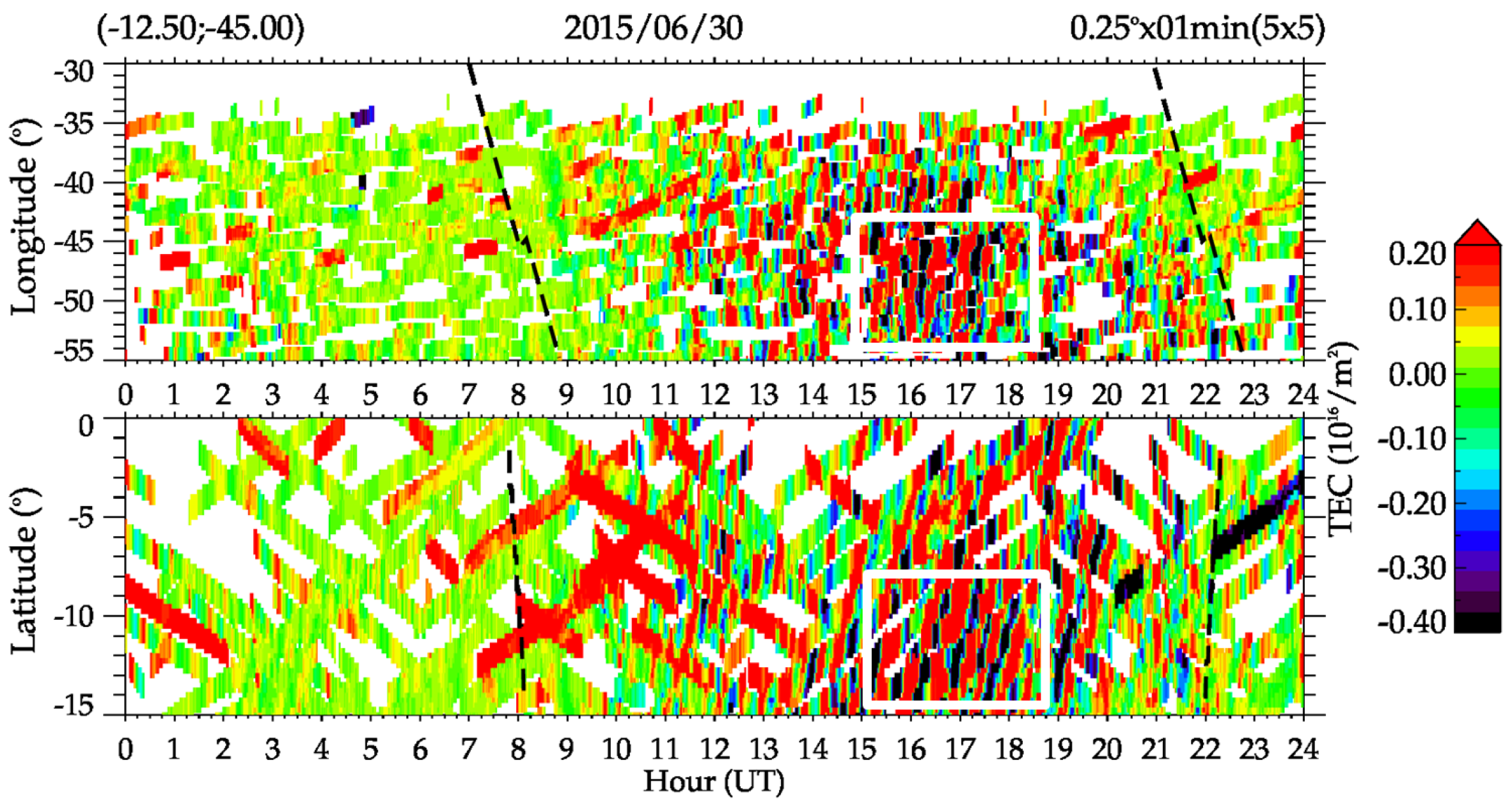
Method of Generating the Two-Dimensional dTEC Maps

Generating dTEC maps requires the corresponding longitude and latitude of ionospheric piercing point (IPP) position, which are estimated in [40,41,42]; where λ r and ϕ r are longitude and latitude of the receiver respectively.
ϕ i p p = s i n 1 s i n ϕ r c o s ( ψ ) + c o s ( ϕ r ) s i n ( ψ ) c o s ( A z )
λ i p p = λ r + s i n 1 s i n ( ψ ) s i n ( A z ) c o s ( ϕ i p p )
The two-dimensional maps of the dTEC, within the area of 30–55 W and 0–15 S, were generated with a temporal resolution of 1 min and a spatial resolution of 0 . 25 × 0 . 25 and 5 × 5 smoothing in longitude and latitude, which results in 1 degree in latitude and longitude, i.e., 1 in 300 km altitude corresponds to approximately 116 km. The color table used has a range of 0.2 to −0.4 TECU. Figure 3 shows an example of dTEC maps over South America on 30 June 2015 at 16:45:00 Universal time (UT = 13:45:00 local time (LT)). The concentric MSTID oscillations can be identified with the red and blue denoting crest (black dashes on top of each) and trough, respectively. On this day, MSTIDs oscillations with wavefront elongated from the northwest to the southeast were observed propagating northeastward between 15:00 UT and 18:00 UT (12:00 LT to 15:00 LT).
The series of dTEC maps were generated at 16:45:00 UT (13:45:00 LT) to observe the propagation of the MSTIDs in the South American region on June 30 2015. For example, Figure 4 shows the dTEC maps from 16:50:00 UT (13:50:00 LT) to 17:05:00 UT (14:05:00 LT) in every 5 min time interval. The animation of Figure 4 is available through the supplementary information related to this manuscript (see Movie_MSTID01).
In order to characterize the MSTIDs into wavelength, propagation direction, period, and phase speed, keograms were created from a series of dTEC maps [35] by taking latitudinal and longitudinal cuts of each dTEC map. For example, a cut was made at latitude 12 . 5 S and longitude 45 . 0 W in every 1 min of the series of dTEC maps generated from 30 June 2015. This technique helps in identifying the oscillations of MSTIDs and their behaviors over 24 h in one single frame. This analytical method has been used in many research works [35,43,44,45,46,47,48]. Figure 5 presents a keogram of the dTECmap; the abscissa is the interval of time and the ordinate is the corresponding distance in geographic coordinates. From the keogram, the MSTID oscillations can be identified with positive (red) and negative (blue) dTEC lines denoting the crest and trough respectively. The black dashed lines indicate the dawn and dusk solar terminator at 300 km altitude.
In order to calculate the wavelength, period, direction of propagation, and phase velocity, we employed a spectral analysis, using discrete Fourier transforms as shown in the appendix of [35] to characterized the MSTIDs. This was done by selecting the area of interest between longitude 40–55 W and latitude 7–14 N against 15:00 to 19:00 UT, as indicated by the white box shown in Figure 5.
The following criteria were considered when analyzing the MSTID characteristics:
  • The direction of propagation was determined by the tilt of the MSTID in the latitudinal and longitudinal components.
  • The propagation direction must be perpendicular to the front of the TID, and the variation azimuth starts from the geographic North ( 0 ) and continues clockwise.
  • The wave phases selected in a particular component should be moving in the same direction.
  • The horizontal wavelength should not exceed 1500 km [6,35].
  • The amplitude of the dTEC oscillation should be more than 0.2 TECU [6].
  • It is requested that the areas to be analyzed are equal and exist in the same time domain in both longitudinal and latitudinal components of the keogram.
  • The time interval for the oscillation(s) should be at least 30 min.
  • The oscillation should have at least two wavefront and propagates on the maps, assuming that the propagation direction is perpendicular to the wavefront of the MSTID.
  • The Wavefront should be greater than 3 in latitude and longitude on the keograms.

3. Results

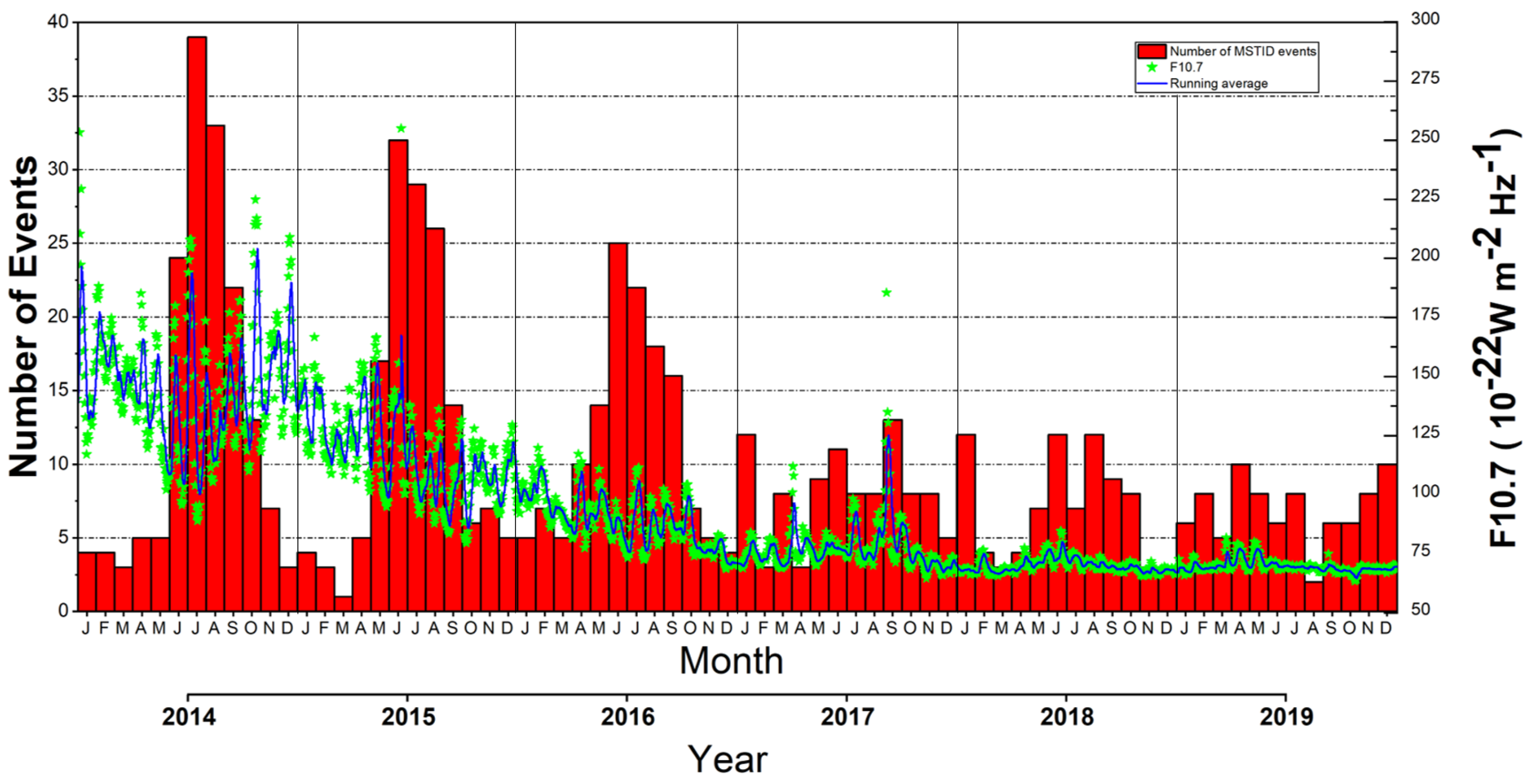
3.1. Occurrence of MSTIDs during Solar Cycle 24

After analyzing the dTEC maps obtained by the GPS and GLONASS receivers in the South American equatorial region from January 2014 to December 2019, we estimated the horizontal wavelength, period, and phase speed of 712 MSTIDs, as well as their local time of occurrence during geomagnetically quiet conditions.
The present study covers half a period of the solar cycle 24 epoch. In order to investigate the possible effects of solar activity on the occurrence rate of MSTID events, we present the climatology of the six-year MSTIDs as shown in Table 1. There is a clear annual variation in the statistical analysis of the MSTID events from the maximum solar phase through the descending phase to the minimum solar phase activity. The MSTID occurrence was the maximum (162 events) in 2014 (solar maximum) and reduced to the half (83 events) in 2019 (solar minimum). It indicates the solar cycle dependency of the events.
To investigate the monthly/seasonal variations of the occurance rate of MSTIDs during the maximum, descending, and minimum solar phases in solar cycle 24, the 6-year dataset was divided into three seasons, equinox (March-May and September-November), summer (December–February), and winter (June–August). The solar flux F10.7 cm and the total MSTID events are plotted as a function of month and year, as shown in Figure 6. The monthly occurrence rate of MSTIDs during geomagnetically quiet conditions is indicated with the red histogram, while the green represents the solar flux (F10.7), and the blue line is the respective eighty-one day running average.
The seasonal variation peaks were around the winter solstice months in all years, with the exception of the minimum solar phase, where the usual winter preferences are not clear. On the other hand, the summer solstice events seem to increase from the solar maximum to minimum. The low-level MSTID activity during the summer months, especially during the maximum solar phase, is a potential interest to study. The occurrence pattern during the equinoxes from 2014–2016 are quite similar, as well as 2017–2019. From Figure 6, it is clear that the strong semiannual variation, winter maximum, and summer minimum during the solar maximum disappeared during the solar minimum phase. We attest to the fact that the present equatorial MSTIDs show a strong positive correlation with the solar activity.

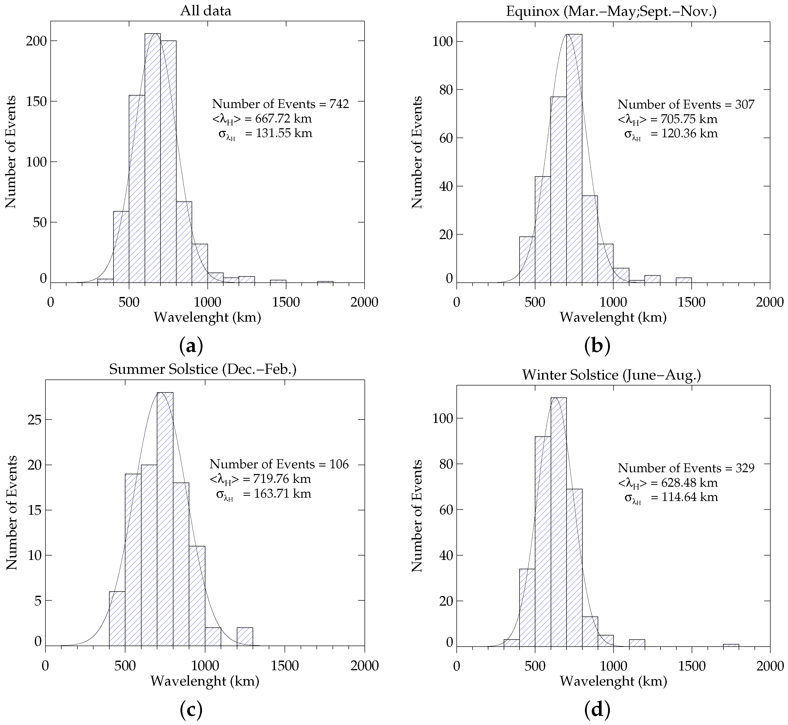
3.2. Horizontal Wavelength of the MSTIDs

In order to investigate the horizontal wavelength of the present work, the number of events is plotted against the horizontal wavelength. Figure 7 shows the horizontal wavelength of the MSTIDs observed over the South American equatorial region for (a) all seasons, (b) equinoxes, (c) summer, and (d) winter, respectively. The horizontal wavelengths are divided into 100 km bins and the solid black line represent the Gaussian fit of the distribution. Most of the horizontal wavelengths in (a), (b), and (d) are between 500 and 800 km and occurred during daytime and evening time, although there are few nighttime events during equinox. In summer, the majority of the events are distributed between 500 and 900 km and occurred during dusk and nighttime with few daytime events, while the winter distribution peaks between 500 and 700 km. The mean values of all, equinoxes, summer, and winter are 667 ± 131 , 705 ± 120 , 719 ± 163 , and 628 ± 114 km for (a), (b), (c), and (d) respectively. The difference of the wavelength between summer and winter is significant, which will be discussed in the next section.

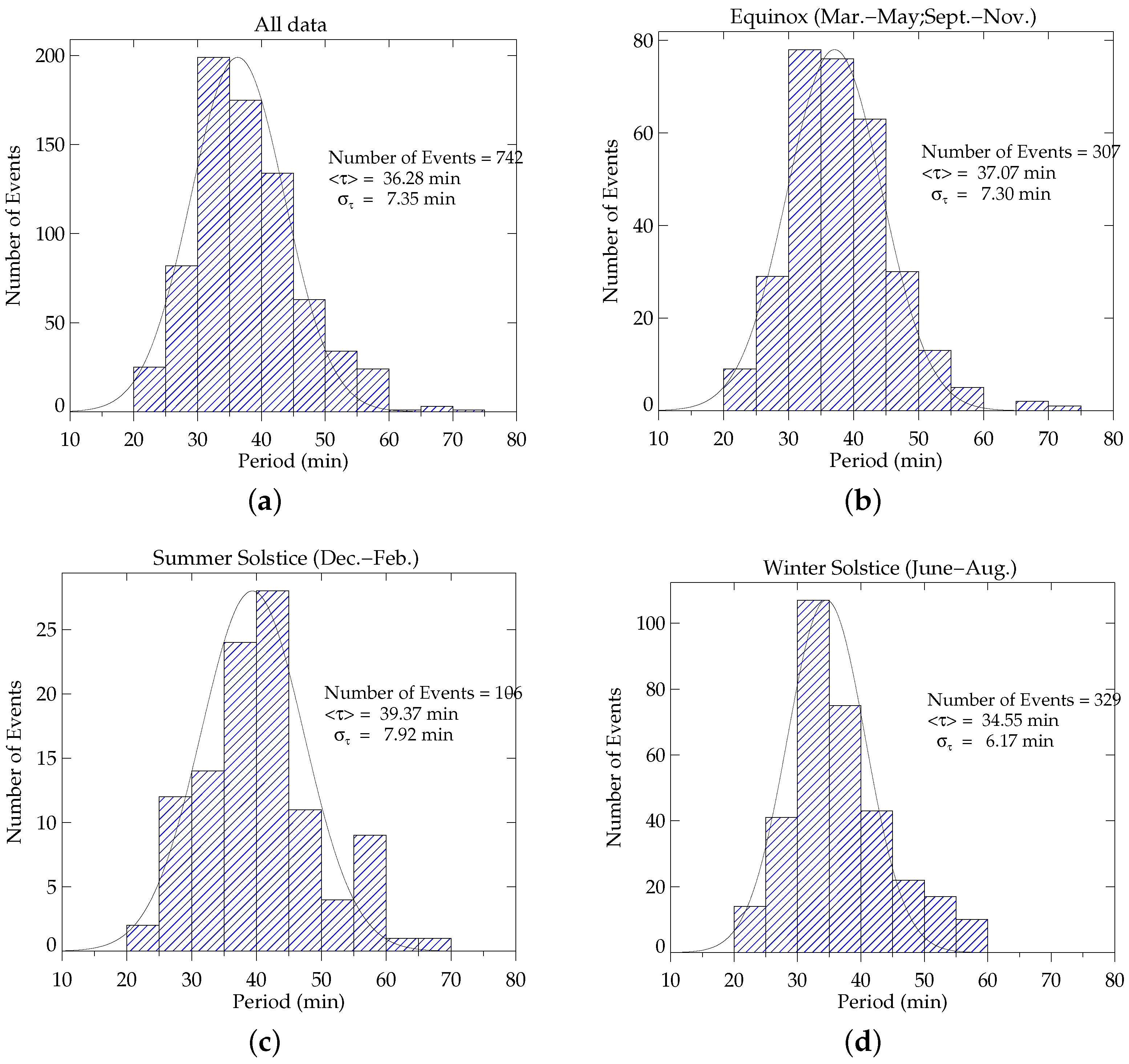
3.3. Period of MSTIDs

The number of event is plotted against the corresponding period of the MSTIDs observed over the South American Equatorial region in Figure 8 for (a) all seasons, (b) equinoxes, (c) summer, and (d) winter. The periods are binned into 10 min intervals. Most of the periods for (a), (b), (c), and (d) range from 20 to 60 min with mean values of 36 ± 7 , 37 ± 7 , 39 ± 7 , and 34 ± 6 min, respectively. In equinoxes, the maximum period is concentrated around 30 to 45 min, while summer and winter are 35 to 45 min and 30 to 40 min, respectively. There is no significant difference of the period between the seasons.

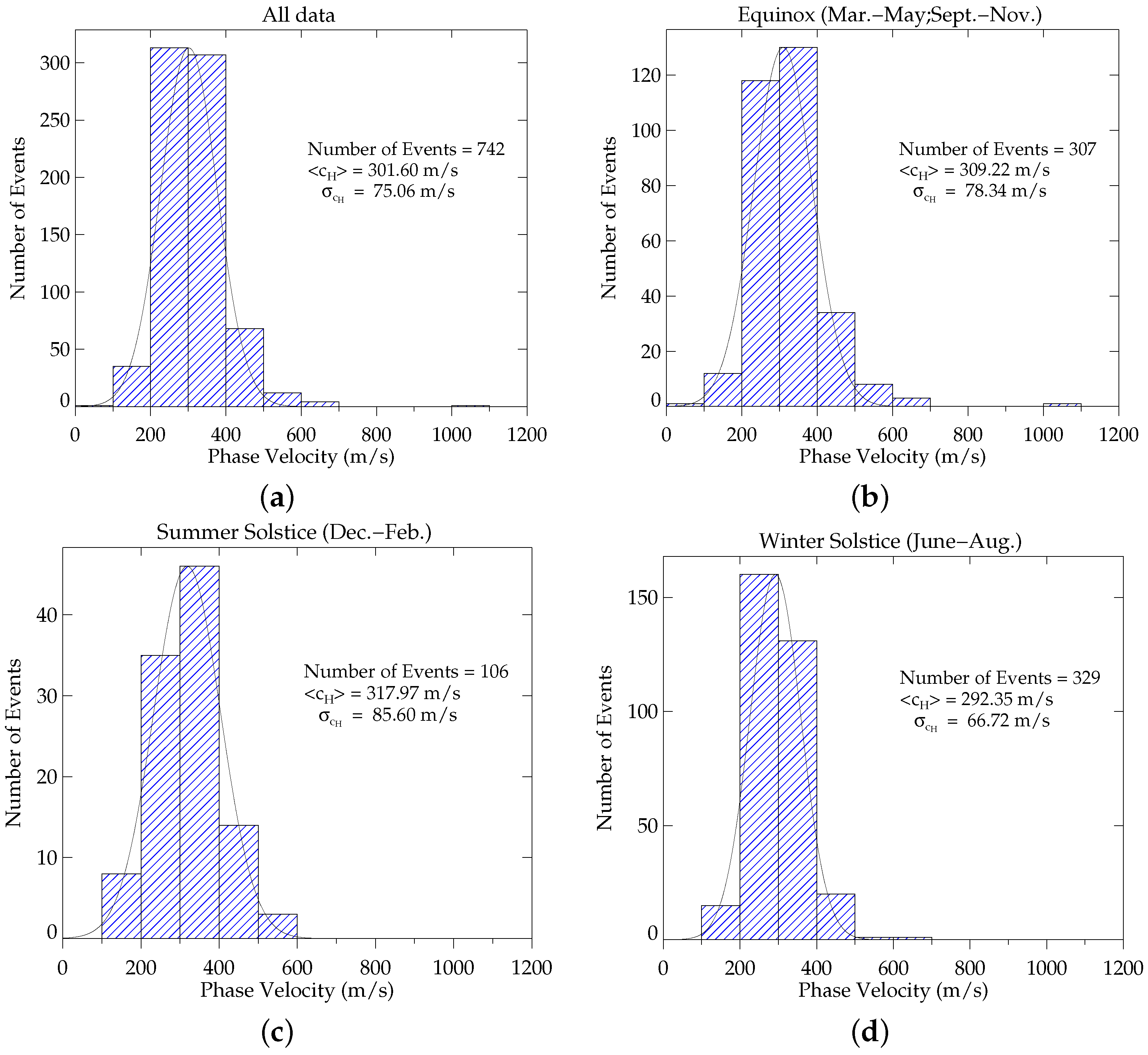
3.4. Horizontal Phase Velocity of the MSTIDs

Figure 9 presents the phase velocities of the MSTIDs observed for (a) all seasons, (b) equinoxes, (c) summer, and (d) winter. The phase velocities are divided into 100 m/s bin. Most of the phase velocities are distributed between 200 and 400 m/s. The (a), (b), and (c) range from 100 to 600 m/s, while the winter is between 100 and 500 m/s. The number of events is highest between 300–400 m/s during summer, while during the winter it is 200–300 m/s. The mean distribution of the horizontal phase velocity for (a), (b), (c), and (d) are 301 ± 60 , 309 ± 78 , 317 ± 85 , and 291 ± 66 m/s, respectively.

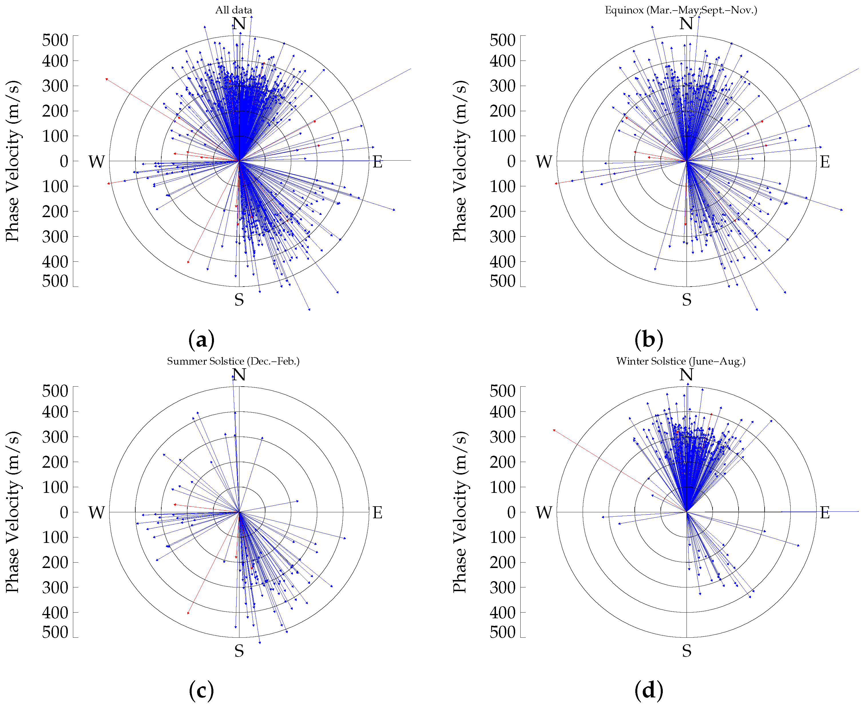
3.5. Propagation Direction of the MSTIDs

Figure 10 shows the propagation direction of the MSTIDs observed as a function of phase velocity from January 2014 to December 2019 for (a) all seasons, (b) equinoxes, (c) summer, and (d) winter. The data was classified into 30 bins and the propagation direction was defined as the angles clockwise from geographical North. As shown in the figure, the red arrows denote the nighttime MSTID events, while the blue arrows are daytime and evening time. We did not find the azimuthal variation of the ocurrence rate of the MSTIDs between daytime and evening events. In the equinoxes, the MSTID activities propagated predominantly in thr north-northeast, north-northwest, and south-southeast directions. In summer, the propagation directions are preferentially south-southeast and a few westward, while in winter they predominantly propagated to the north-northeast and north-northwest directions with few southeastward. There is a significant difference between summer and winter events in their propagation directions. The few nighttime events captured did not show any preferential propagation direction.

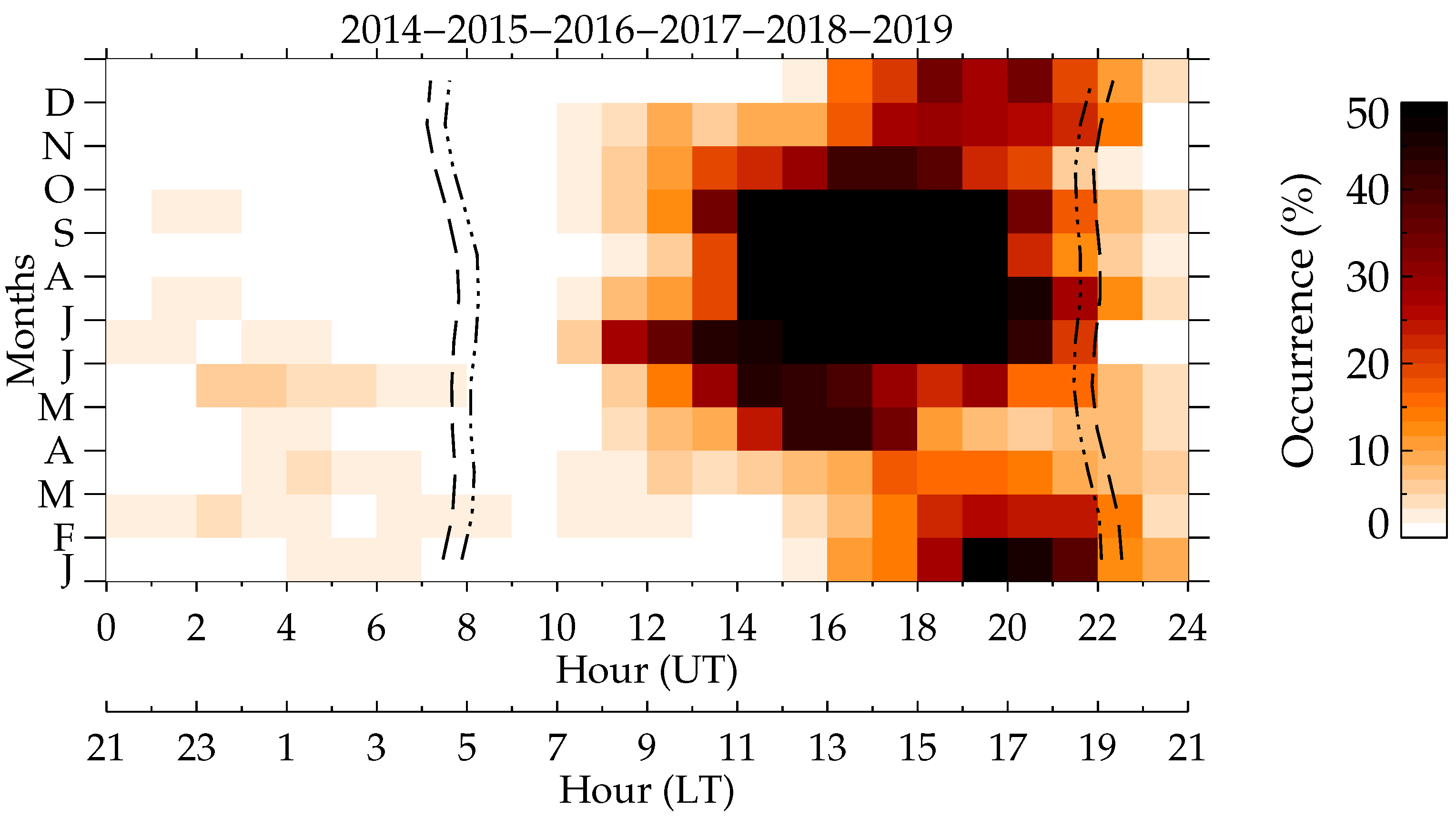
3.6. Local Time Dependence of the Equatorial MSTID

Figure 11 show the local time and seasonal variations of the MSTID occurrence rate in monthly and hourly bins. The months are represented by their initials, while the dawn and dusk solar terminator are shown at the altitude of 100 km and 300 km as dotted and broken lines, respectively. The occurrence rate is defined as the ratio of the time of the MSTID to the monthly and hourly observation intervals. It should be noted in the present work that the MSTID occurrence in the South American equatorial region strongly depends on the local time. The occurrence rates are classified into daytime (7:00–17:00 LT), evening time (17:00–20:00 LT), and nighttime (21:00–4:00). A high occurrence rate can be seen during the daytime, which mostly occurs in winter months with a secondary peak in the equinoctial months. The evening events are seen in winter and summer months with minor peak in equinoctial months. There is no clear seasonality in the nighttime events. The occurrence rate in daytime is ∼80% of the total number of MSTIDs observed, while the evening MSTID is ∼18%, and the nighttime accounted for only ∼2% of the total MSTIDs observed. The occurrence of MSTIDs near the dawn terminator side in the present work was rare.

4. Discussion

Using GPS and GLONASS data obtained over the South American equatorial region from January 2014–December 2019, we developed TEC perturbation maps that identify the presence of MSTIDs. A total of 712 MSTIDs were detected during geomagnetically quiet time, and their aforementioned characteristics were calculated. The statistical analysis of the equatorial MSTIDs is presented with respect to the solar minimum, descending, and maximum phases.

4.1. Characteristics of the Equatorial MSTIDs

The horizontal wavelengths observed in the present work were concentrated between 500 and 800 km with a mean value of 667 ± 131 km; the periods peaked around 30 to 45 min with a mean value of 37 ± 7 min; and the majority of the horizontal phase velocities had values between 200 and 400 m/s with a mean of 301 ± 75 m/s. The main difference between the present work and previous works by [35] among others, is the fact that the present horizontal wavelengths are much higher, although, they were conducted using the same GNSS dTEC map and 1 h running average technique. Furthermore, the phase speeds of the present equatorial MSTIDs and those observed by [35] in the southeast of Brazil are similar but faster than those observed by [7,11,49]. Ref. [34] reported MSTIDs with periods of 20–35 min and opposite directions of propagation, depending on the hemisphere in the South American equatorial region; however, the focus was on only magneto-conjugated TIDs of the equatorial region.
In the midlatitude, ref. [11] reported MSTIDs with horizontal wavelength, period, and phase velocity ranging between 100 and 450 km, 20 to 60 min, and 50 to 200 m/s, respectively, using dTEC maps; while [7] used dTEC maps to observe the Japanese sector and reported MSTIDs with horizontal wavelength, period, and phase velocity ranging from 100 to 600 km, 15 to 60 min, and 50 to 300 m/s, respectively. In the low-latitude region over China, ref. [49] used the Hong Kong Continuously Operating Reference Stations network to record MSTIDs with the horizontal wavelength, phase speed, and period in the spring, autumn, and winter daytime (from 10:00 to 17:00 LT) between 250 and 450 km, 140 and 240 m/s, and 20 and 50 min, while these data and between 200 and 450 km, and 220 m/s, and 30 and 45 min in the spring and summer nighttime (from 22:00 to 03:00 LT), respectively. Ref. [33] also used ionosonde to observe the MSTIDs horizontal phase velocities between 150 and 300 m/s. In the southeast of Brazil ( 15 to 30 S), ref. [35] used GPS dTEC maps to study MSTIDs and observed the horizontal wavelength, period, and phase speed between 200 and 1000 km, 15 and 35 min, 100 and 600 m/s with the mean values of 445 ± 106 km, 23 ± 3 min, and 322 ± 80 m/s, respectively.
The seasonal propagation direction of summer and winter suggests a consistent cyclic picture with predominantly northward propagation during the winter months and transitioning to south-southeastward during the summer periods. In winter, the propagation direction of [35] is only northwards, while that of the present work was northward and south-southeastward. However, in summer, the propagation direction of MSTIDs observed by [35], propagated in all directions, while that of the present work is predominantly southeastward. Meanwhile, the propagation directions in the equinox of the two works are similar. The winter and summer propagation direction demonstrates a strong link between the MSTIDs observed in the southeast of Brazil by [35] and the present work. For example, it is possible that most of the observed equatorial MSTIDs propagated northward in the present work during winter have their sources in the low latitude. Similarly, the dominant southeastward MSTIDs during summer might have been triggered by the gravity waves that were generated by intertropical convergence zone (ITCZ) [33,50], which lies with the study area during summer, and migrates to the north in winter.
These equatorial MSTIDs were likely induced by the secondary or tertiary gravity waves created in the thermosphere from the dissipation of primary gravity waves that were excited from deep convection in the troposphere [51,52]. The present characteristics are consistent with the TIDs. Ref. [52] studied at the bottomside of the F layer (230–290 km) observed by the TIDDBIT ionospheric sounder with periods between 15 and 90 min, horizontal wavelengths of 100 and 3000 km, and horizontal phase speeds of 140 to 650 m/s. In the case of the South American continent, ref. [53] used a gravity wave resolving the global circulation model (GCM) to investigate the effects on the mesosphere and thermosphere from a strong mountain wave (MW) event over the Southern Andes during the winter. They reported that those gravity waves broke and attenuated at an altitude of 50–80 km, thereby creating local body forces that generated large-scale secondary gravity waves having concentric ring structure with horizontal wavelengths between 500 and 2000 km, horizontal phase speeds from 70 to 100 m/s, and periods of 3 to 10 h, and can consequently break and generate tertiary gravity waves, which then propagated to the northeast of Brazil.

4.2. Seasonal Variation of Equatorial MSTIDs

As presented in the previous section, we observed a strong seasonal variation in the frequency of occurrence, summer minimum, and winter maximum. This tendency is much stronger in the period of the solar maximum (2014–2016). Concerning this, there were two factors to be considered, one is seasonal variation of gravity wave activity in the middle atmosphere, and the other is the gravity wave filtering mechanism in the lower thermosphere.
The MSTIDs predominantly occur during daytime in winter and nighttime in summer with a secondary peak in the equinoxes. From the present statistical analysis, we realized that the number of observed equatorial MSTIDs were 286, 97, and 329 for equinoxes, summer, and winter, respectively. Our present results are consistent with [35,49] and mid latitudes [5,6,7,11]. Atmospheric gravity waves and their propagation characteristics in relation to the mean flow, such as background wind, might be crucial to the seasonal variation of the present equatorial MSTIDs. The earliest observations of the traveling ionospheric disturbances conducted by [54,55,56] led [9] to hypothesize that TIDs were the manifestations of neutral internal gravity waves in the ionospheric plasma; this has been generally accepted today. The medium-scale gravity waves are known to transport energy and momentum throughout the atmospheric layers, resulting in a coupling between them [45,48,57].
To explain the influence of background wind in the current seasonal variation of the equatorial MSTIDs, we adopted the dispersion relation of gravity waves equation with negligible dissipation, ion drag, and wave-induced diffusion [58], as shown Equation (7). This equation also allows for the ray tracing of gravity waves from the lower atmosphere into the thermosphere and ionosphere [52]. Where m is the vertical wave number, N is the Brunt V a ¨ i s a ¨ l a ¨ frequency, c horizontal phase speed of the gravity waves, u is the neutral wind velocity, and k is the horizontal wave number.
m 2 = N 2 c u 2 k 2 1 4 H 2
In the work of [59] on the thermospheric winds and temperatures in the northeast of Brazil, it was reported that while the temperature climatology shows the expected solar cycle dependence, the neutral winds are most heavily dominated by seasonal change. During summer, the velocity of the neutral wind, u, is higher than in winter. Hence, c u will be smaller, resulting in a larger vertical wave number, m. From the dispersion-relation equation for gravity waves, the vertical wave number will be larger in summer than in winter, and eventually the vertical wavelength could be larger in winter than in summer. Gravity waves with larger vertical wave numbers are dissipated due to the high viscosity and thermal conductivity in the thermosphere [12,60].
In this regard, the gravity waves could be filtered out by the critical level or dissipated in the thermosphere due to high viscosity [48,52]. As a result, a few gravity waves with longer wavelength and higher phase speed are likely to propagate into the ionospheric level as MSTIDs in summer, which consequently minimizes the number of MSTIDs activities in the season. On the other hand, in winter, the neutral wind velocity u is slow and lesser than any of the phase velocities of the MSTID in the present work. Hence, c u will be larger, resulting in a small vertical wave number m. In this case, the gravity waves could propagate into the thermosphere/ionosphere without critical level effect or dissipation caused by high thermospheric viscosity [52].
Ref. [61] reported that the energy of the gravity waves at 120 km altitude was slightly high but much higher at 300 km altitude during winter; however, in summer, the gravity waves lacked the ability to propagate vertically upward. They further reported that the zonal wind filtering effect between 100 and 200 km altitude is the mechanism that normally blocks the vertical propagation of the gravity waves. This implies that the high frequency gravity waves with high energy generated in the troposphere are capable of propagating into the thermosphere to induce wave structures in the ionosphere during winter or were excited by secondary and tertiary gravity waves in the thermosphere from the likely dissipated primary gravity waves triggered by deep convection sources in the troposphere.
The source mechanism that generated gravity waves in the troposphere could contribute to the seasonal variations of the present equatorial MSTIDs statistics. For example, ref. [35] reported that in winter there is a strong cold front emanating from the mid and high latitudes, which extends to the low latitudes. Ref. [53] also reported that medium- and large-scale daytime secondary and tertiary gravity waves, which were likely Mountain waves with concentric ring structures from the Southern Andes, are possible to excite MSTIDs that propagate north-northeastward over the Brazilian region. Ref. [48] observed medium-scale gravity waves propagating northeastward, which were likely generated by the deep convective source over the Amazon region that are capable of propagating to the ionospheric level. These sources are the possible proxy for the gravity waves that likely excited the north-northeastward and north-northwestward MSTIDs observed over the South American equatorial region. The penetrative cumulus convection in the ITCZ was the most likely generation mechanism of the gravity waves that excited the summer MSTIDs, which predominantly propagated southeastward [33,50].

4.3. Long Term Variability of Equatorial MSTIDs

The percentage occurrence rate of equatorial MSTIDs for the 6-year study were 43.3%, 33.7%, and 23.0% for the maximum (2014–2015), descending (2016–2017), and minimum (2018–2019) solar phases, respectively. The daytime climatology of the equatorial MSTIDs show their dependence on solar activities; hence, for the first time we report the positive trend of the equatorial MSTID occurrence and solar activities in the South American equatorial region. Once again, the annual variation of the present work is more applicable to the daytime MSTID, since ∼70% were observed during the daytime. Ref. [8] first studied MSTIDs across the globe during the solar descending (1998) and maximum (2000 and 2001) phase, and reported that the nighttime MSTID activity at the Japanese and Australian longitudinal sectors show negative correlation with the solar activity; whereas, solar activity dependence was not seen in the daytime MSTID activity. Ref. [62] also studied MSTIDs over California, New Zealand, Alaska, and Hawaii during solar maximum conditions and reported that most of the MSTID climatological trends were modulated by the solar cycle intensity. The inverse dependence of the occurrence of nighttime MSTIDs in relation to solar activity has previously been reported by [20,21,63,64,65] in the mid and low latitudes.
Ref. [57] report a strong solar cycle effect on gravity wave propagation into the thermosphere, and that they can propagate to higher altitudes during high sunspot activity relative to minimum conditions. Ref. [3] further reported that gravity waves can propagate to higher altitudes during high sunspot activity conditions, more than during solar minimum conditions. This implies that there is a strong solar cycle effect on gravity wave propagation into the thermosphere. Therefore, solar cycle effects on gravity wave propagation might have caused the decreasing rate of MSTIDs from January 2014 (solar maximum) to December 2019 (solar minimum).
Another factor that could be a possible contributor is the gravity wave propagation characteristics in relation to the thermospheric temperature and viscosity. The thermospheric temperature determines the viscosity of the medium and is highly dense during the solar minimum and consequent increase in the dissipative gravity waves, hence impeding their propagation into the thermosphere/ionosphere. According to [66], the dissipation rates due to thermospheric viscosity and thermal conduction are inversely proportional to the neutral gas density. This dissipation rate depends on the temperature structure of the thermosphere, which consequently affects the wave group velocity. That is, a hotter thermosphere refracts the wave energy at more oblique angles and hence, increases the dissipation rate. Therefore, the gravity wave dissipation depends strongly on local time and solar activity [66].
From the dispersion relation Equation (7) of the gravity waves, ref. [52] reported that in the absence of dissipation, the vertical wavelength of gravity wave increases by T ¯ / T 0 ¯ or greater if its intrinsic frequency is close to the smaller thermospheric buoyancy frequency N = T ¯ / T 0 ¯ N 0 , where T ¯ and T 0 ¯ are the asymptotic temperatures in the thermosphere and lower atmosphere, respectively. They, however, mention that in the presence of dissipation, vertical wavelength increases in the thermosphere during active solar conditions, which is more applicable during the solar maximum. However, during the extreme solar minimum, there is negligible forcing above an altitude of 230 km, and this forcing extends up to 360 km altitude during active solar conditions. Ref. [67] also reported that medium-scale gravity waves in the thermosphere with high frequency and long vertical wavelength components penetrate into the highest altitudes.
In order to investigate the thermospheric temperature in relation to the dissipation of gravity waves in the thermosphere, we plotted altitude as a function of temperature using values from the NRLMSIS-00 model as shown in Figure 12. Each line represents the profiles of average neutral temperature for a particular year as indicated in the plot. While the thermospheric temperature during solar minimum is ∼650 K, that of the maximum phase is ∼950 K. It is clear that the temperature variation between the solar maximum and minimum in the thermosphere is wide enough to influence the dissipative difference between the solar phases. Ref. [68] reported that the basic structure of thermospheric neutral winds above about 150 km altitude is formed by atmospheric expansion due to solar heating on the dayside, creating a pressure bulge with a temperature maximum developing near 14:00 LT. This establishes the fact that there is high viscosity in the thermosphere, which leads to high dissipation of gravity waves during low solar activity.
Ref. [69] reported that the increase in temperatures associated with the increase in solar flux was seen in the progression of temperature from 2009 through 2012, which is consistent with the results of [59] in the same equatorial region over Brazil. From the thermospheric viscosity analogy they discussed using modelled and observational temperature data, gravity waves could dissipate due to high viscosity in the thermosphere, which is frequent during the solar minimum. This implies that during the solar minimum, only gravity waves with longer vertical wavelength and higher phase velocity can exist or survive to induced MSTIDs in the thermposphere [12]. With respect to the thermospheric temperature data during the solar maximum and minimum phases observed by [59,69], we could establish the connection between the solar activities and the gravity wave dissipation due to thermospheric viscosity as the precursor of the wide variation of the occurrence rate of the present MSTIDs.
Although, some of the values of the MSTIDs are above the supersonic speed, it’s still possible that the high viscosity condition in the thermosphere during the solar descending and minimum phase filtered out most of the gravity wave events with low speed. Ref. [70] reported that the gravity wave vertical wavelength (m) in the thermosphere is larger than in the lower atmosphere, and this increase is much larger when the sun is active than when the sun is quiet. This, of course, can minimizes the dissipation rate of gravity waves in the thermosphere during high solar activities, thereby, propagating into the ionospheres as TIDs. This could also be the possible reason for the positive correlation of the MSTID occurrence rate in solar cycle 24.

5. Conclusions

We have analyzed data collected by the GNSS dual frequency receivers network to develope detrended TEC maps that identify and characterize the medium-scale traveling ionospheric disturbances (MSTIDs) over the South American equatorial region (latitude: 0 to 15 S and longitude: 30 to 55 W ). Statistical analysis of the occurrence rate of MSTIDs during the solar maximum phase, descending phase, and minimum phase has been carried out over the South American region. Furthermore, the seasonal variability of occurrence of the MSTIDs, their horizontal wavelengths, periods, phase velocities, and propagation direction were calculated. We found out that:
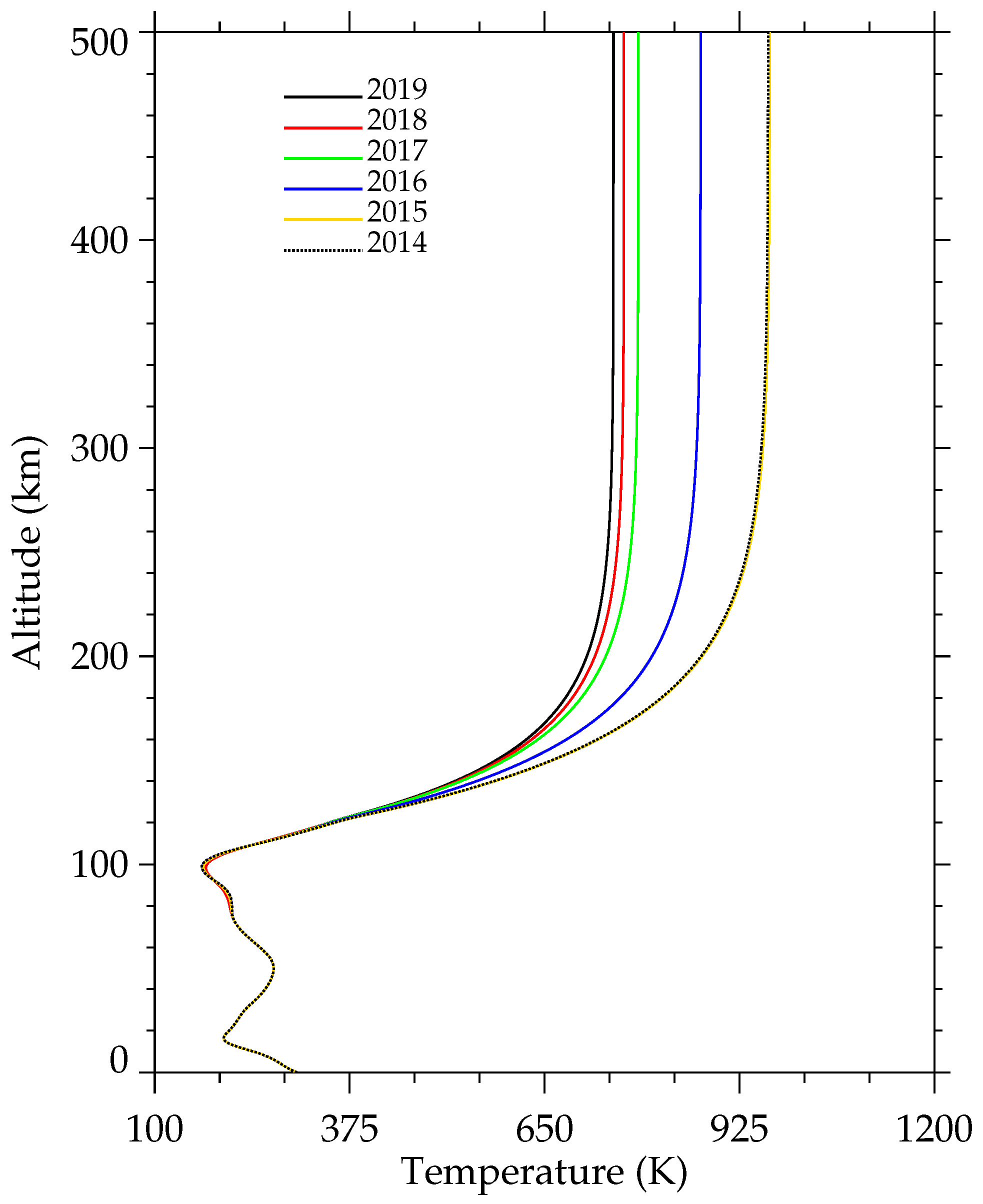
  • A total of 712 MSTIDs were observed during geomagnetic quiet conditions and the statistical analysis was done during the solar cycle 24 (from January 2014 to December 2019). The number of MSTIDs observed increases with the solar activity; that is, most of the them were observed during the solar maximum phase and decrease in the minimum phase. This might have been caused by gravity wave dissipation due to high viscosity in the thermosphere as a result of low and high thermospheric temperature during solar minimum and maximum, respectively.
  • The predominant daytime MSTIDs representing 80% of the total observation occurred in winter with the secondary peak in the equinox, while the evening time MSTID, which is 18% of the entire events, occurred in summer and equinox, and the remaining 2% of the MSTIDs were observed during nighttime. The seasonal variation of the MSTID events was attributed to the source mechanisms generating them, the wind filtering and dissipation effect, and the local time dependency.
  • The horizontal wavelengths of the MSTIDs were mostly concentrated between 500 and 800 km, with a mean value of 667 ± 131 km. The observed periods ranged from 30 to 45 min, with a mean value of 36 ± 7 min. The observed horizontal phase speeds were distributed around 200 to 400 m/s, with coarresponding mean of 301 ± 75 m/s.
  • The MSTIDs in the winter solstice and equinoctial months preferentially propagated northeastward and northwestward. Meanwhile, during the summer solstice they propagated in all directions. The anisotropy of the propagation direction might be due to several reasons: the wind and dissipative filtering effects, ion drag effects, primary source region, and the presence of the secondary or tertiary gravity waves in the thermosphere. The atmospheric gravity waves from strong convective sources originated from the equatorial and Amazon region might be the primary precursor of the northeastward and northwestward propagating MSTIDs during the summer solstice and autumn equinox. Nevertheless, the strong cold front emanating from the low latitude might have been the primary source for the northeastward and northwestward MSTIDs during the winter solstice and spring equinox. In all seasons, we noted that the MSTIDs propagating southeastward were probably excited by the likely gravity waves generated by the ITCZ.

Supplementary Materials

The following are available online at https://www.mdpi.com/article/10.3390/atmos12111409/s1, Video S1: Movie_MSTID01.

Author Contributions

Conceptualization, P.E., C.A.O.B.F., C.M.W., H.T. and D.G.; methodology, C.A.O.B.F., C.M.W., D.B. and H.T.; software, C.A.O.B.F., C.M.W. and D.B.; validation, C.A.O.B.F., H.T., C.M.W., D.B., A.V.B. and S.O.L.; formal analysis, C.A.O.B.F., H.T. and S.O.L.; investigation, C.A.O.B.F., H.T., D.B., T.T.A. and S.O.L.; resources, H.T., C.A.O.B.F., N.A.B.K.; data curation, C.A.O.B.F.; writing—original draft preparation, H.T., C.A.O.B.F., C.M.W., S.O.L., N.A.B.K., T.T.A. and A.V.B.; writing—review and editing, P.E., H.T., C.A.O.B.F., N.A.B.K., C.M.W., S.O.L. and T.T.A. All authors have read and agreed to the published version of the manuscript.

Funding

This research was initially funded by Nacional de Desenvolvimento Cientifico e Tecnologico” (CNPq), project no. 141044/2017-9 and “Coordenacao de Aperfeicoamento de Pessoal de Nivel Superior” (CAPES). The drafting of the paper and publication expenses are funded by African Institute for Mathematical Sciences (AIMS) Rwanda.

Institutional Review Board Statement

Not applicable.

Informed Consent Statement

Not applicable.

Data Availability Statement

The data used in this paper can be access from the official website of the RMBC, RAMSAC, LISN and IGS as well as National Institute for Space Research (INPE) EMBRACE.

Acknowledgments

With the deepest gratitude, I wish to appreciate the financial support and institutional framework of the “Conselho Nacional de Desenvolvimento Cientifico e Tecnologico” (CNPq), project no. 141044/2017-9 and “Coordenacao de Aperfeicoamento de Pessoal de Nivel Superior” (CAPES) for the PhD scholarship as well as providing free accessibility for several online journals. C.A.O.B. Figueiredo thanks “Fundação de Amparo à Pesquisa do Estado de São Paulo (FAPESP)” under the process 2018/09066-8 and 2019/22548-4 and the National Institute for Space Research (INPE) including São Paulo Research Foundation (FAPESP). Diego Barros also thank “Conselho Nacional de Desenvolvimento Cientifico e Tecnológico (CNPq) under the process 301988/2021-8”. We thank all the institutes that own the GNSS receivers network over South America: RBMC (Brazilian Institute of Geography and Statistics, Brazil), RAMSAC (National Geographic Institute, Argentina), CORS (National Geodetic Survey, USA), IGS (International GNSS Service) and UNAVCO (National Science Foundation, USA and National Atmospheric and Space Administration, USA), for making available the RINEXs files, substantial for obtaining the results. We are grateful to the Brazilian Space Climate Study and Monitoring program (EMBRACE) for making RINEX files available. I also thank the American Geophysical Union (AGU) for the Max Hammond Student Travel Grant Award for good abstract to participate in the 2019 AGU Fall Meeting in San Francisco, CA, U.S.A. I thank the Committee on Space Research (COSPAR) for granting me the opportunity to participate in Capacity Building Workshop on Space Weather in 2018 at INPE and awarding my group for best presentation. My appareciation to African Institute for Mathematical Sciences (AIMS) Ghana and Rwanda for providing me all I need during the drafting of this paper.

Conflicts of Interest

The authors of this current work, solemnly declare no conflict of interest as far as the entire work is concerned.

References

  1. Hunsucker, R.; Delana, B.; Hargreaves, J. ATS-6 RBE measurements of ionospheric storm-time behaviour of TEC and other parameters at College, Alaska. In International Symposium on Beacon Satellite Studies of the Earth’s Environment; National Physical Laboratory of India: New Delhi, India, 1984; pp. 467–477. [Google Scholar]
  2. Francis, S.H. A theory of medium-scale traveling ionospheric disturbances. J. Geophys. Res. 1974, 79, 5245–5260. [Google Scholar] [CrossRef]
  3. Crowley, G.; Azeem, I. Extreme Ionospheric Storms and Their Effects on GPS Systems. In Extreme Events in Geospace; Elsevier: Amsterdam, The Netherlands, 2018; pp. 555–586. [Google Scholar]
  4. Squat, K.; Schlegel, K. A review of atmospheric gravity waves and travelling ionospheric disturbances: 1982–1995. Ann. Geophys. 1996, 14, 917. [Google Scholar]
  5. Tsugawa, T.; Otsuka, Y.; Coster, A.J.; Saito, A. Medium-scale traveling ionospheric disturbances detected with dense and wide TEC maps over North America. Geophys. Res. Lett. 2007, 34. [Google Scholar] [CrossRef]
  6. Otsuka, Y.; Suzuki, K.; Nakagawa, S.; Nishioka, M.; Shiokawa, K.; Tsugawa, T. GPS observations of medium-scale traveling ionospheric disturbances over Europe. Ann. Geophys. 2013, 31, 163–172. [Google Scholar] [CrossRef]
  7. Otsuka, Y.; Kotake, N.; Shiokawa, K.; Ogawa, T.; Tsugawa, T.; Saito, A. Statistical study of medium-scale traveling ionospheric disturbances observed with a GPS receiver network in Japan. In Aeronomy of the Earth’s Atmosphere and Ionosphere; Abdu, M.A., Pancheva, D., Eds.; Springer: Dordrecht, The Netherlands, 2011; pp. 291–299. [Google Scholar]
  8. Kotake, N.; Otsuka, Y.; Tsugawa, T.; Ogawa, T.; Saito, A. Climatological study of GPS total electron content variations caused by medium-scale traveling ionospheric disturbances. J. Geophys. Res. Space Phys. 2006, 111. [Google Scholar] [CrossRef]
  9. Hines, C.O. Internal atmospheric gravity waves at ionospheric heights. Can. J. Phys. 1960, 38, 1441–1481. [Google Scholar] [CrossRef]
  10. Miller, C.A. Electrodynamics of midlatitude spread F 2. A new theory of gravity wave electric fields. J. Geophys. Res. Space Phys. 1997, 102, 11533–11538. [Google Scholar] [CrossRef]
  11. Kotake, N.; Otsuka, Y.; Ogawa, T.; Tsugawa, T.; Saito, A. Statistical study of medium-scale traveling ionospheric disturbances observed with the GPS networks in Southern California. Earth Planets Space 2007, 59, 95–102. [Google Scholar] [CrossRef] [Green Version]
  12. Otsuka, Y.; Shinbori, A.; Tsugawa, T.; Nishioka, M. Solar activity dependence of medium-scale traveling ionospheric disturbances using GPS receivers in Japan. Earth Planets Space 2021, 73, 1–11. [Google Scholar] [CrossRef]
  13. Perkins, F. Spread F and ionospheric currents. J. Geophys. Res. 1973, 78, 218–226. [Google Scholar] [CrossRef]
  14. Otsuka, Y.; Onoma, F.; Shiokawa, K.; Ogawa, T.; Yamamoto, M.; Fukao, S. Simultaneous observations of nighttime medium-scale traveling ionospheric disturbances and E region field-aligned irregularities at midlatitude. J. Geophys. Res. Space Phys. 2007, 112. [Google Scholar] [CrossRef]
  15. Hernandez-Pajares, M.; Juan, J.M.; Sanz, J. Medium-scale traveling ionospheric disturbances affecting GPS measurements: Spatial and temporal analysis. J. Geophys. Res. Space Phys. 2006, 111. [Google Scholar] [CrossRef]
  16. Kintner, P.M.; Ledvina, B.M.; De Paula, E.R. GPS and ionospheric scintillations. Space Weather 2007, 5. [Google Scholar] [CrossRef]
  17. Takahashi, H.; Wrasse, C.M.; Figueiredo, C.A.O.B.; Barros, D.; Abdu, M.A.; Otsuka, Y.; Shiokawa, K. Equatorial plasma bubble seeding by MSTIDs in the ionosphere. Prog. Earth Planet. Sci. 2018, 5, 32. [Google Scholar] [CrossRef] [Green Version]
  18. Takahashi, H.; Wrasse, C.; Figueiredo, C.; Barros, D.; Paulino, I.; Essien, P.; Abdu, M.; Otsuka, Y.; Shiokawa, K. Equatorial plasma bubble occurrence under propagation of MSTID and MLT gravity waves. J. Geophys. Res. Space Phys. 2020, 125, e2019JA027566. [Google Scholar] [CrossRef]
  19. Retterer, J.; Roddy, P. Faith in a seed: On the origins of equatorial plasma bubbles. Ann. Geophys. 2014, 32, 485–498. [Google Scholar] [CrossRef] [Green Version]
  20. Pimenta, A.A.; Kelley, M.C.; Sahai, Y.; Bittencourt, J.A.; Fagundes, P.R. Thermospheric dark band structures observed in all-sky OI 630 nm emission images over the Brazilian low-latitude sector. J. Geophys. Res. Space Phys. 2008, 113. [Google Scholar] [CrossRef] [Green Version]
  21. Candido, C.M.N.; Pimenta, A.A.; Bittencourt, J.A.; Becker-Guedes, F. Statistical analysis of the occurrence of medium-scale traveling ionospheric disturbances over Brazilian low latitudes using OI 630.0 nm emission all-sky images. Geophys. Res. Lett. 2008, 35. [Google Scholar] [CrossRef] [Green Version]
  22. Makela, J.J.; Miller, E.S.; Talaat, E.R. Nighttime medium-scale traveling ionospheric disturbances at low geomagnetic latitudes. Geophys. Res. Lett. 2010, 37. [Google Scholar] [CrossRef]
  23. Amorim, D.C.M.; Pimenta, A.A.; Bittencourt, J.A.; Fagundes, P.R. Long-term study of medium-scale traveling ionospheric disturbances using OI 630 nm all-sky imaging and ionosonde over Brazilian low latitudes. J. Geophys. Res. Space Phys. 2011, 116. [Google Scholar] [CrossRef] [Green Version]
  24. Paulino, I.; Medeiros, A.F.; Vadas, S.L.; Wrasse, C.M.; Takahashi, H.; Buriti, R.A.; Leite, D.; Filgueira, S.; Bageston, J.V.; Sobral, J.H.A.; et al. Periodic waves in the lower thermosphere observed by OI630 nm airglow images. Ann. Geophys. 2016, 34, 293–301. [Google Scholar] [CrossRef] [Green Version]
  25. Machado, C.S. Estudo de Distúrbios Ionosféricos Propagantes de Média Escala no Hemisfério sul Utilizando Técnicas óticas, de Rádio e Simulações Numéricas. Ph.D. Thesis, Instituto Nacional de Pesquisas Espaciais (INPE), São José dos Campos, Brazil, 2017. [Google Scholar]
  26. Figueiredo, C.; Takahashi, H.; Wrasse, C.M.; Otsuka, Y.; Shiokawa, K.; Barros, D. Investigation of Nighttime MSTIDS Observed by Optical Thermosphere Imagers at Low Latitudes: Morphology, Propagation Direction, and Wind Filtering. J. Geophys. Res. Space Phys. 2018, 139, 7843–7857. [Google Scholar] [CrossRef]
  27. Tsugawa, T.; Saito, A.; Otsuka, Y. A statistical study of large-scale traveling ionospheric disturbances using theGPS network in Japan. J. Geophys. Res. Space Phys. 2004, 109. [Google Scholar] [CrossRef]
  28. Otsuka, Y.; Shiokawa, K.; Ogawa, T.; Wilkinson, P. Geomagnetic conjugate observations of medium-scale traveling ionospheric disturbances at midlatitude using all-sky airglow imagers. Geophys. Res. Lett. 2004, 31. [Google Scholar] [CrossRef]
  29. Shiokawa, K.; Otsuka, Y.; Ogawa, T. Quasiperiodic southward moving waves in 630-nm airglow images in the equatorial thermosphere. J. Geophys. Res. Space Phys. 2006, 111. [Google Scholar] [CrossRef] [Green Version]
  30. Fukushima, D.; Shiokawa, K.; Otsuka, Y.; Ogawa, T. Observation of equatorial nighttime medium-scale traveling ionospheric disturbances in 630-nm airglow images over 7 years. J. Geophys. Res. Space Phys. 2012, 117. [Google Scholar] [CrossRef] [Green Version]
  31. Saito, A.; Fukao, S.; Miyazaki, S. High resolution mapping of TEC perturbations with the GSI GPS network over Japan. Geophys. Res. Lett. 1998, 25, 3079–3082. [Google Scholar] [CrossRef]
  32. Ding, F.; Wan, W.; Xu, G.; Yu, T.; Yang, G.; Wang, J.S. Climatology of medium-scale traveling ionospheric disturbances observed by a GPS network in central China. J. Geophys. Res. Space Phys. 2011, 116. [Google Scholar] [CrossRef]
  33. MacDougall, J.; Abdu, M.A.; Batista, I.; Buriti, R.; Medeiros, A.F.; Jayachandran, P.T.; Borba, G. Spaced transmitter measurements of medium scale traveling ionospheric disturbances near the equator. Geophys. Res. Lett. 2011, 38. [Google Scholar] [CrossRef] [Green Version]
  34. Jonah, O.F.; Kherani, E.A.; De Paula, E.R. Investigations of conjugate MSTIDS over the Brazilian sector during daytime. J. Geophys. Res. Space Phys. 2017, 122, 9576–9587. [Google Scholar] [CrossRef]
  35. Figueiredo, C.; Takahashi, H.; Wrasse, C.; Otsuka, Y.; Shiokawa, K.; Barros, D. Medium-scale traveling ionospheric disturbances observed by detrended total electron content maps over Brazil. J. Geophys. Res. Space Phys. 2018, 123, 2215–2227. [Google Scholar] [CrossRef]
  36. Mannucci, A.J.; Wilson, B.D.; Yuan, D.N.; Ho, C.H.; Lindqwister, U.J.; Runge, T.F. A global mapping technique for GPS-derived ionospheric total electron content measurements. Radio Sci. 1998, 33, 565–582. [Google Scholar] [CrossRef]
  37. Boucher, C.; Altamimi, Z. ITRS, PZ-90 and WGS 84: Current realizations and the related transformation parameters. J. Geod. 2001, 75, 613–619. [Google Scholar] [CrossRef]
  38. Cai, C.; Gao, Y. A combined GPS/GLONASS navigation algorithm for use with limited satellite visibility. J. Navig. 2009, 62, 671–685. [Google Scholar] [CrossRef]
  39. Goral, W.; Skorupa, B. Determination of intermediate orbit and position of GLONASS satellites based on the generalized problem of two fixed centers. Acta Geodyn. Geromater. 2012, 9, 283–291. [Google Scholar]
  40. Otsuka, Y.; Ogawa, T.; Saito, A.; Tsugawa, T.; Fukao, S.; Miyazaki, S. A new technique for mapping of total electron content using GPS network in Japan. Earth Planets Space 2002, 54, 63–70. [Google Scholar] [CrossRef]
  41. Basu, S.; Basu, S.; Valladares, C.E.; Yeh, H.C.; Su, S.Y.; MacKenzie, E.; Sultan, P.J.; Aarons, J.; Rich, F.J.; Doherty, P.; et al. Ionospheric effects of major magnetic storms during the International Space Weather Period of September and October 1999: GPS observations, VHF/UHF scintillations, and in situ density structures at middle and equatorial latitudes. J. Geophys. Res. Space Phys. 2001, 106, 30389–30413. [Google Scholar] [CrossRef] [Green Version]
  42. Prol, F.d.S.; Camargo, P.d.O.; Muella, M.T.d.A.H. Comparative study of methods for calculating ionospheric points and describing the gnss signal path. Bol. Ciências Geodésicas 2017, 23, 669–683. [Google Scholar] [CrossRef] [Green Version]
  43. Sobral, J.H.A.; Takahashi, H.; Abdu, M.A.; Taylor, M.J.; Sawant, H.; Santana, D.C.; Gobbi, D.; de Medeiros, A.F.; Zamlutti, C.J.; Schuch, N.J.; et al. Thermospheric F-region travelling disturbances detected at low latitude by an OI 630 nm digital imager system. Adv. Space Res. 2001, 27, 1201–1206. [Google Scholar] [CrossRef]
  44. Saito, S.; Yamamoto, M.; Hashiguchi, H.; Maegawa, A.; Saito, A. Observational evidence of coupling between quasi-periodic echoes and medium-scale traveling ionospheric disturbances. Ann. Geophys. 2007, 25, 2185–2194. [Google Scholar] [CrossRef]
  45. Taylor, M.J.; Pautet, P.D.; Medeiros, A.; Buriti, R.; Fechine, J.; Fritts, D.; Vadas, S.; Takahashi, H.; Sao Sabbas, F. Characteristics of mesospheric gravity waves near the magnetic equator, Brazil, during the SpreadFEx campaign. Ann. Geophys. 2009, 27, 461. [Google Scholar] [CrossRef] [Green Version]
  46. Paulino, I.; Takahashi, H.; Gobbi, D.; Medeiros, A.; Buriti, R.; Wrasse, C. Observações de ondas de gravidade de média escala na região equatorial do Brasil. In Proceedings of the 12th International Congress of the Brazilian Geophysical Society & EXPOGEF, Rio de Janeiro, Brazil, 15–18 August 2011; pp. 2123–2126. [Google Scholar]
  47. Narayanan, V.L.; Shiokawa, K.; Otsuka, Y.; Saito, S. Airglow observations of nighttime medium-scale traveling ionospheric disturbances from Yonaguni: Statistical characteristics and low-latitude limit. J. Geophys. Res. Space Phys. 2014, 119, 9268–9282. [Google Scholar] [CrossRef]
  48. Essien, P.; Paulino, I.; Wrasse, C.M.; Campos, J.A.V.; Paulino, A.R.; Medeiros, A.F.; Buriti, R.A.; Takahashi, H.; Agyei-Yeboah, E.; Lins, A.N. Seasonal characteristics of small-and medium-scale gravity waves in the mesosphere and lower thermosphere over the Brazilian equatorial region. Ann. Geophys. 2018, 36, 899–914. [Google Scholar] [CrossRef] [Green Version]
  49. Chen, G.; Zhou, C.; Liu, Y.; Zhao, J.; Tang, Q.; Wang, X.; Zhao, Z. A statistical analysis of medium-scale traveling ionospheric disturbances during 2014–2017 using the Hong Kong CORS network. Earth Planets Space 2019, 71, 1–14. [Google Scholar] [CrossRef]
  50. Röttger, J. Travelling disturbances in the equatorial ionosphere and their association with penetrative cumulus convection. J. Atmos. Terr. Phys. 1977, 39, 987–998. [Google Scholar] [CrossRef]
  51. Vadas, S.L.; Crowley, G. Sources of the traveling ionospheric disturbances observed by the ionospheric TIDDBIT sounder near Wallops Island on 30 October 2007. J. Geophys. Res. Space Phys. 2010, 115. [Google Scholar] [CrossRef]
  52. Vadas, S.L.; Fritts, D.C. Influence of solar variability on gravity wave structure and dissipation in the thermosphere from tropospheric convection. J. Geophys. Res. Space Phys. 2006, 111. [Google Scholar] [CrossRef] [Green Version]
  53. Vadas, S.L.; Becker, E. Numerical modeling of the generation of tertiary gravity waves in the mesosphere and thermosphere during strong mountain wave events over the Southern Andes. J. Geophys. Res. Space Phys. 2019, 124, 7687–7718. [Google Scholar] [CrossRef]
  54. Munro, G. Short-period changes in the F region of the ionosphere. Nature 1948, 162, 886–887. [Google Scholar] [CrossRef]
  55. Munro, G. Travelling disturbances in the ionosphere. Proc. R. Soc. Lond. Ser. A. Math. Phys. Sci. 1950, 202, 208–223. [Google Scholar]
  56. Munro, G. Travelling Ionospheric Disturbances in the F region. Aust. J. Phys. 1958, 11, 91–112. [Google Scholar] [CrossRef] [Green Version]
  57. Vadas, S.L.; Taylor, M.J.; Pautet, P.D.; Stamus, P.; Fritts, D.C.; Liu, H.L.; São Sabbos, F.; Batista, V.; Takahashi, H.; Rampinelli, V. Convection: The likely source of the medium-scale gravity waves observed in the OH airglow layer near Brasilia, Brazil, during the SpreadFEx campaign. Ann. Geophys. 2009, 27, 231. [Google Scholar] [CrossRef] [Green Version]
  58. Gossard, E.E.; Hooke, W.H. Waves in the Atmosphere: Atmospheric Infrasound and Gravity Waves-Their Generation and Propagation; Elsevier Scientific Publishing Co.: Amsterdam, The Netherlands, 1975; Volume 2. [Google Scholar]
  59. Fisher, D.J.; Makela, J.J.; Meriwether, J.W.; Buriti, R.A.; Benkhaldoun, Z.; Kaab, M.; Lagheryeb, A. Climatologies of nighttime thermospheric winds and temperatures from Fabry-Perot interferometer measurements: From solar minimum to solar maximum. J. Geophys. Res. Space Phys. 2015, 120, 6679–6693. [Google Scholar] [CrossRef] [Green Version]
  60. Pitteway, M.L.V.; Hines, C.O. The viscous damping of atmospheric gravity waves. Can. J. Phys. 1963, 41, 1935–1948. [Google Scholar] [CrossRef]
  61. Miyoshi, Y.; Fujiwara, H.; Jin, H.; Shinagawa, H. A global view of gravity waves in the thermosphere simulated by a general circulation model. J. Geophys. Res. Space Phys. 2014, 119, 5807–5820. [Google Scholar] [CrossRef]
  62. Hernandez-Pajares, M.; Juan, J.M.; Sanz, J.; Aragon-Angel, A. Propagation of medium-scale traveling ionospheric disturbances at different latitudes and solar cycle conditions. Radio Sci. 2012, 47. [Google Scholar] [CrossRef] [Green Version]
  63. Bowman, G.G. A review of some recent work on mid-latitude spread-F occurrence as detected by ionosondes. J. Geomagn. Geoelectr. 1990, 42, 109–138. [Google Scholar] [CrossRef] [Green Version]
  64. Garcia, F.; Kelley, M.; Makela, J.; Huang, C.S. Airglow observations of mesoscale low-velocity traveling ionospheric disturbances at midlatitudes. J. Geophys. Res. Space Phys. 2000, 105, 18407–18415. [Google Scholar] [CrossRef]
  65. Shiokawa, K.; Ihara, C.; Otsuka, Y.; Ogawa, T. Statistical study of nighttime medium-scale traveling ionospheric disturbances using midlatitude airglow images. J. Geophys. Res. Space Phys. 2003, 108. [Google Scholar] [CrossRef]
  66. Cole, K.D.; Hickey, M.P. Energy transfer by gravity wave dissipation. Adv. Space Res. 1981, 1, 65–75. [Google Scholar] [CrossRef]
  67. Vincent, R.A. The dynamics of the mesosphere and lower thermosphere: A brief review. Prog. Earth Planet. Sci. 2015, 2, 1–13. [Google Scholar] [CrossRef] [Green Version]
  68. Rishbeth, H. Thermospheric winds and the F-region: A review. J. Atmos. Terr. Phys. 1972, 34, 1–47. [Google Scholar] [CrossRef]
  69. Makela, J.J.; Fisher, D.J.; Meriwether, J.W.; Buriti, R.A.; Medeiros, A.F. Near-continual ground-based nighttime observations of thermospheric neutral winds and temperatures over equatorial Brazil from 2009 to 2012. J. Atmos. Sol.-Terr. Phys. 2013, 103, 94–102. [Google Scholar] [CrossRef]
  70. Richmond, A. Gravity wave generation, propagation, and dissipation in the thermosphere. J. Geophys. Res. Space Phys. 1978, 83, 4131–4145. [Google Scholar] [CrossRef]
Figure 1. Distribution of the GNSS ground receivers network. RMBC, RAMSAC, LISN, and IGS are represented by red, blue, violet, and green, respectively.
Atmosphere 12 01409 g001
Figure 2. Vertical TEC (upper panel) with elevation greater than 30 and the corresponding dTEC (lower panel).
Atmosphere 12 01409 g002
Figure 3. Detrending TEC (dTEC) maps with 1 min resolution over South America equatorial region 30 June 2014 at 16:45:00 UT (13:45:00 LT).
Atmosphere 12 01409 g003
Figure 4. The series of dTEC maps on 30 June 2015 from 16:50:00 UT (13:50:00 LT) to 17:05:00 UT (14:05:00 LT) in every 5 min time interval.
Atmosphere 12 01409 g004
Figure 5. The keograms created from dTEC maps on 30 June 2015; longitudinal (top) and latitudinal (bottom). The black dashed lines indicate the dawn and dusk solar terminator.
Atmosphere 12 01409 g005
Figure 6. Solar cycle 24 dependence on occurrence. The monthly occurrence rate of the MSTIDs are indicated by the red histogram; the green represents the solar flux (F10.7), while the blue is the respective eigthy-one day average.
Atmosphere 12 01409 g006
Figure 7. The horizontal wavelength distribution of the MSTIDs observed between January 2014 and December 2019 for (a) all seasons, (b) equinoxes, (c) summer, and (d) winter.
Atmosphere 12 01409 g007
Figure 8. Distribution of the observed period of the MSTIDs observed between January 2014 and December 2019 for (a) all seasons, (b) equinoxes, (c) summer, and (d) winter.
Atmosphere 12 01409 g008
Figure 9. The horizontal phase velocity distribution of the observed medium-scale traveling ionospheric disturbances for (a) all seasons, (b) equinoxes, (c) summer, and (d) winter.
Atmosphere 12 01409 g009
Figure 10. The propagation direction of the observed medium-scale traveling ionospheric disturbances for (a) all seasons, (b) equinoxes, (c) summer, and (d) winter. The red arrows indicate the nighttime MSTID events while that of the blue are daytime and dusk.
Atmosphere 12 01409 g010
Figure 11. Time dependence and seasonal variation of the occurrence of MSTIDs observed over the South American equatorial region from January 2014 to December 2019. The months are represented by their initials and the dawn and dusk solar terminator are shown at the altitude of 100 km (dotted lines) and 300 km (broken line).
Atmosphere 12 01409 g011
Figure 12. Thermospheric neutral temperature profiles from 2014 to 2019 by the NRLMSIS-00 model atmosphere.
Atmosphere 12 01409 g012
Table 1. The annual occurrence rate of MSTIDs during geomagnetically quiet conditions from 2014 to 2019.
YearSolar Cycle PhaseMSTID events
2014Maximum162
2015Maximum146
2016Descending139
2017Descending96
2018Minimum86
2019Minimum83
Publisher’s Note: MDPI stays neutral with regard to jurisdictional claims in published maps and institutional affiliations.

