
Evaluation of F10.7, Sunspot Number and Photon Flux Data for Ionosphere TEC Modeling and Prediction Using Machine Learning Techniques


Abstract
:1. Introduction
2. Features Evaluation
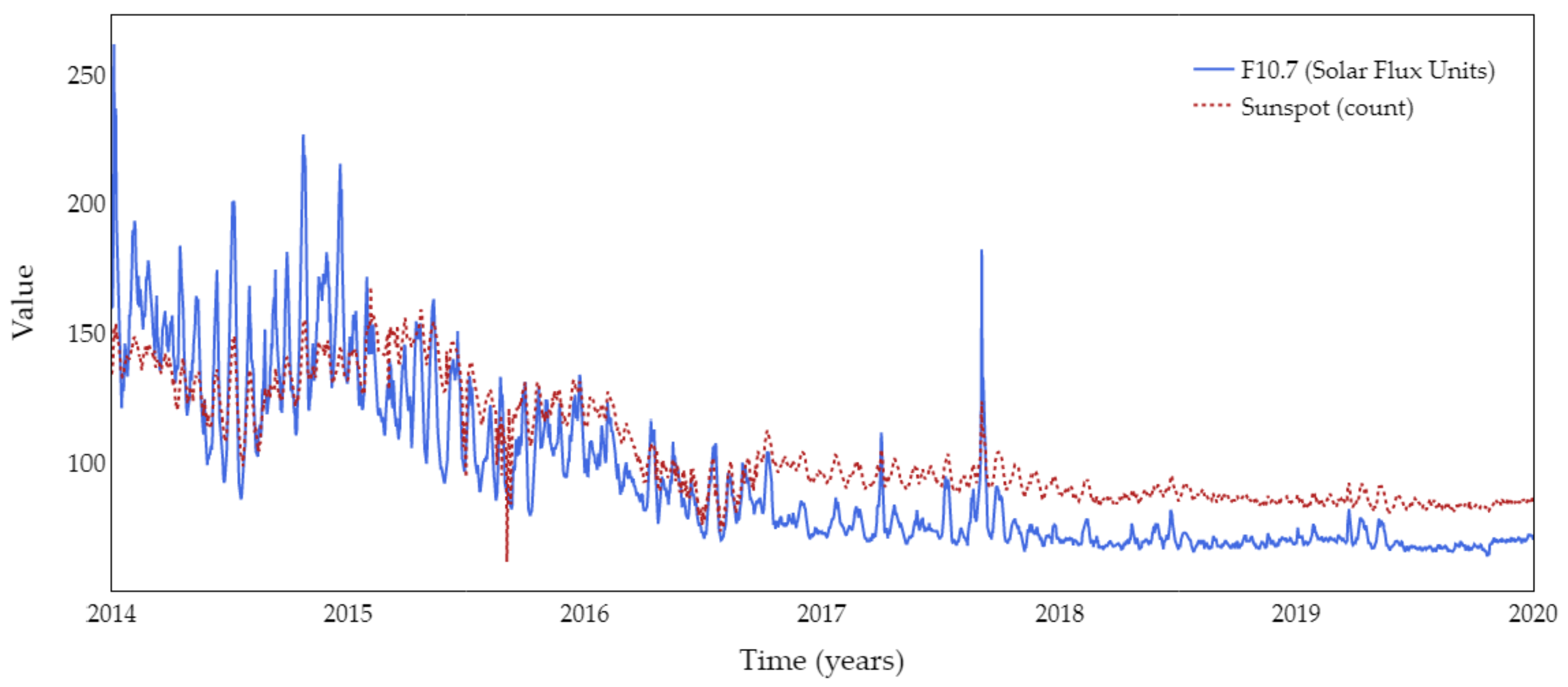
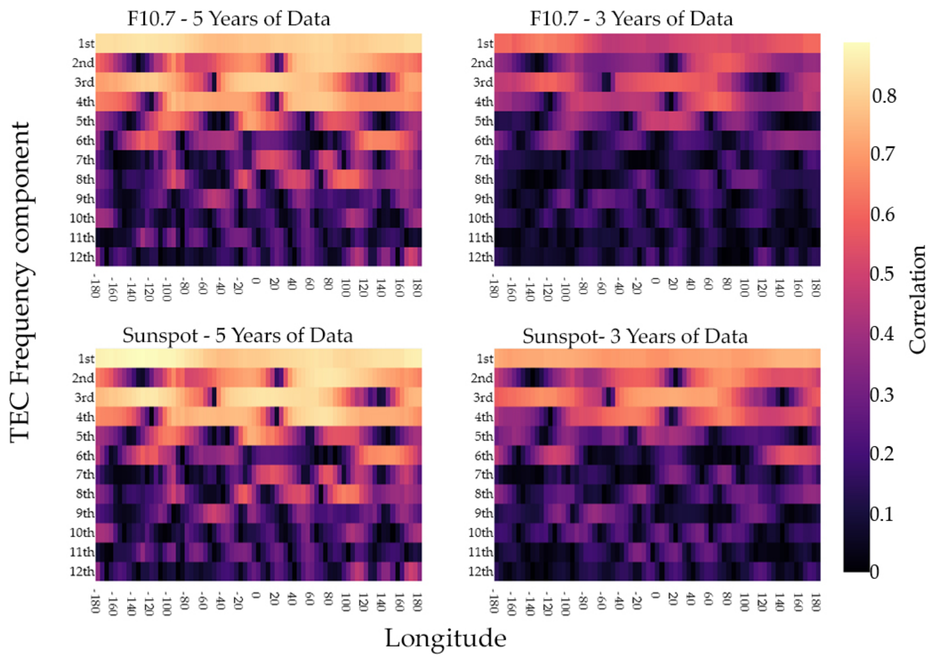
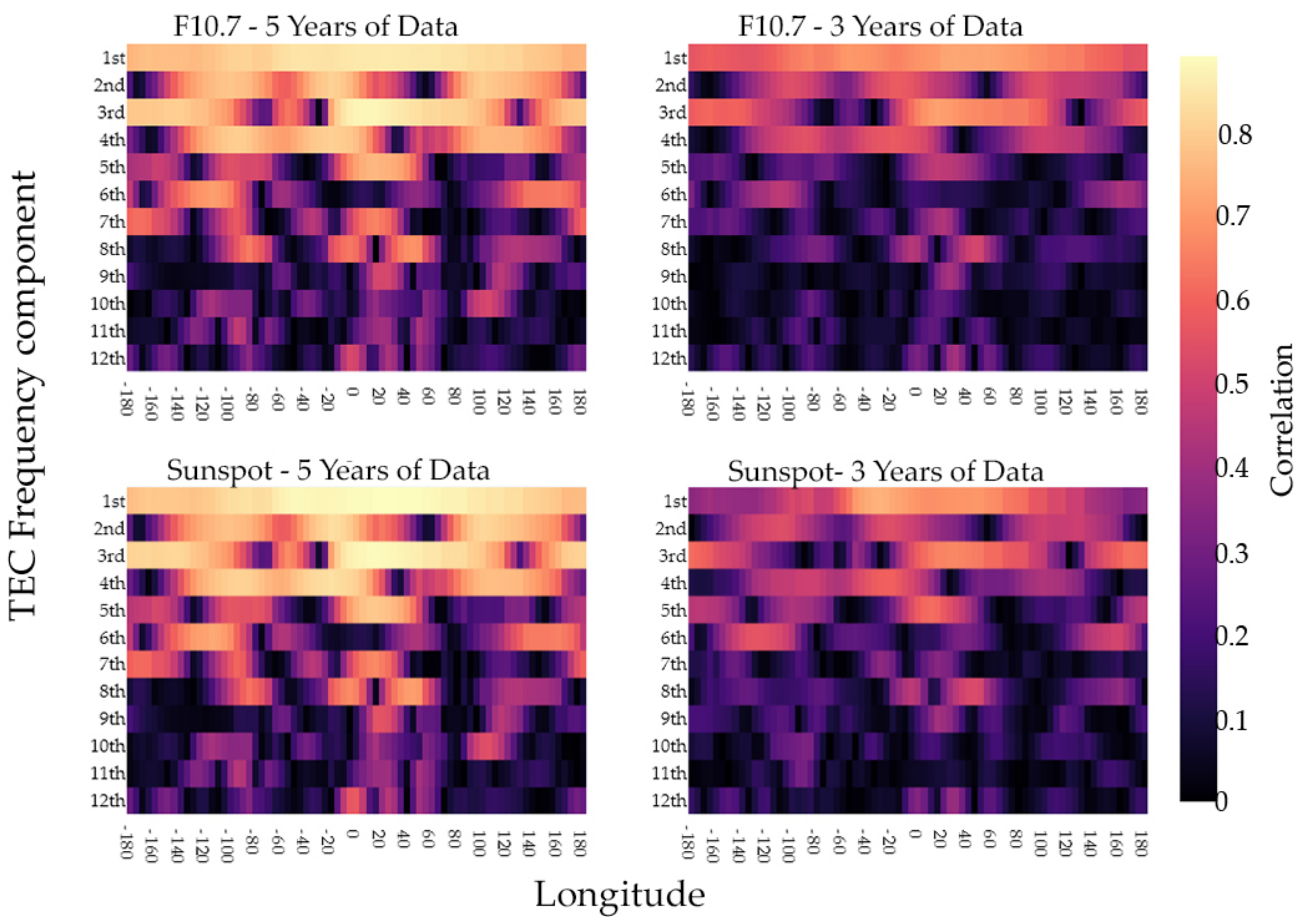
2.1. F10.7
2.2. Sunspot Number
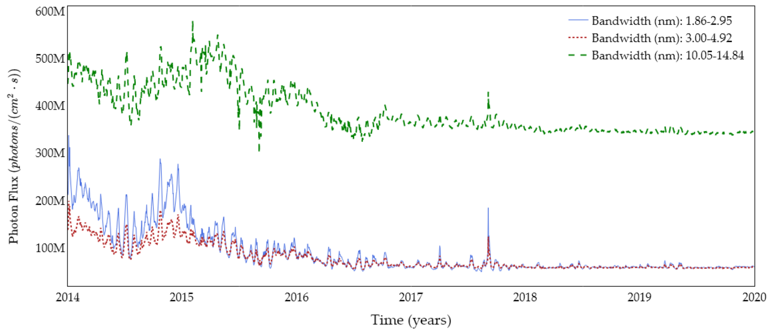
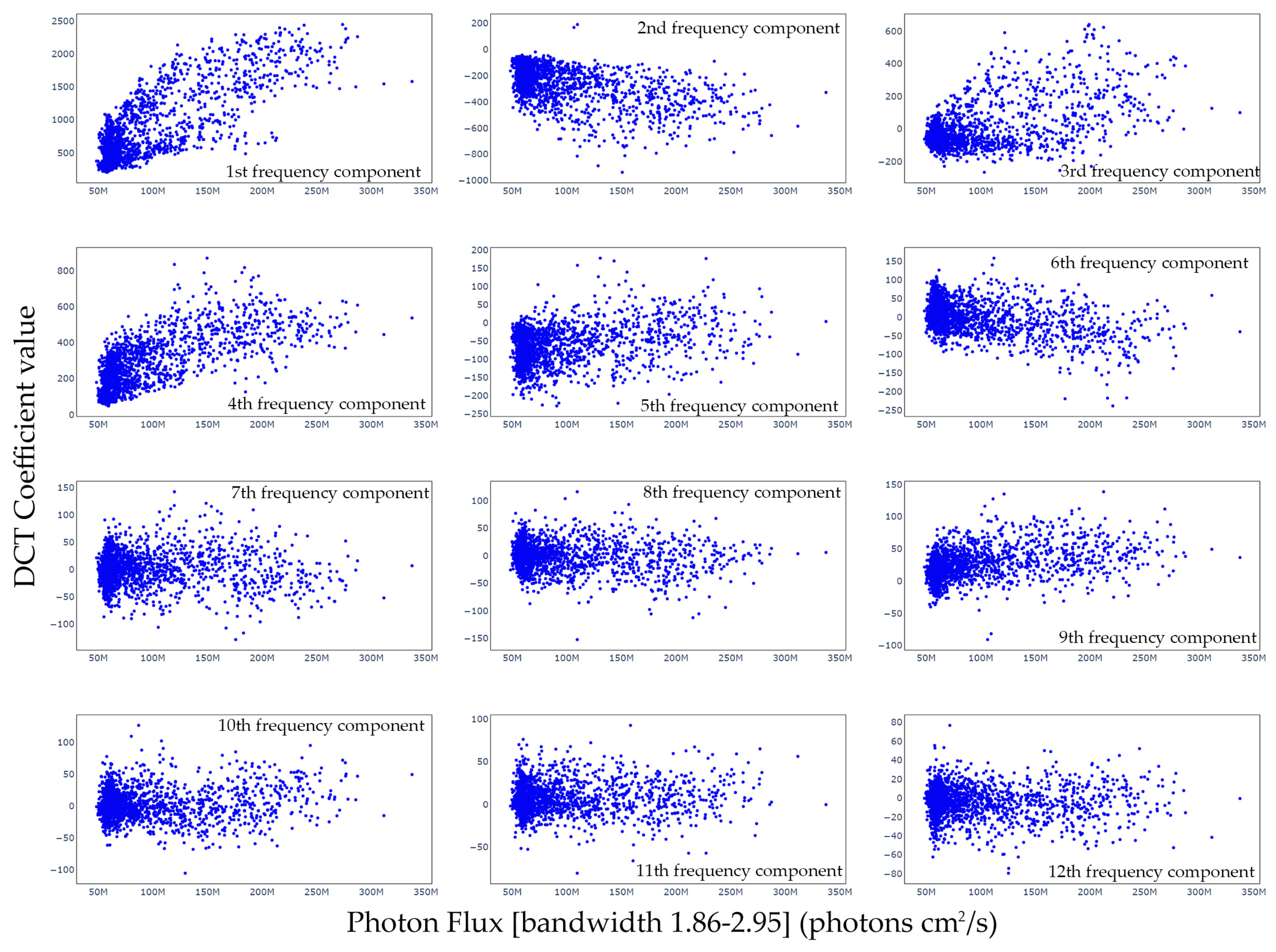
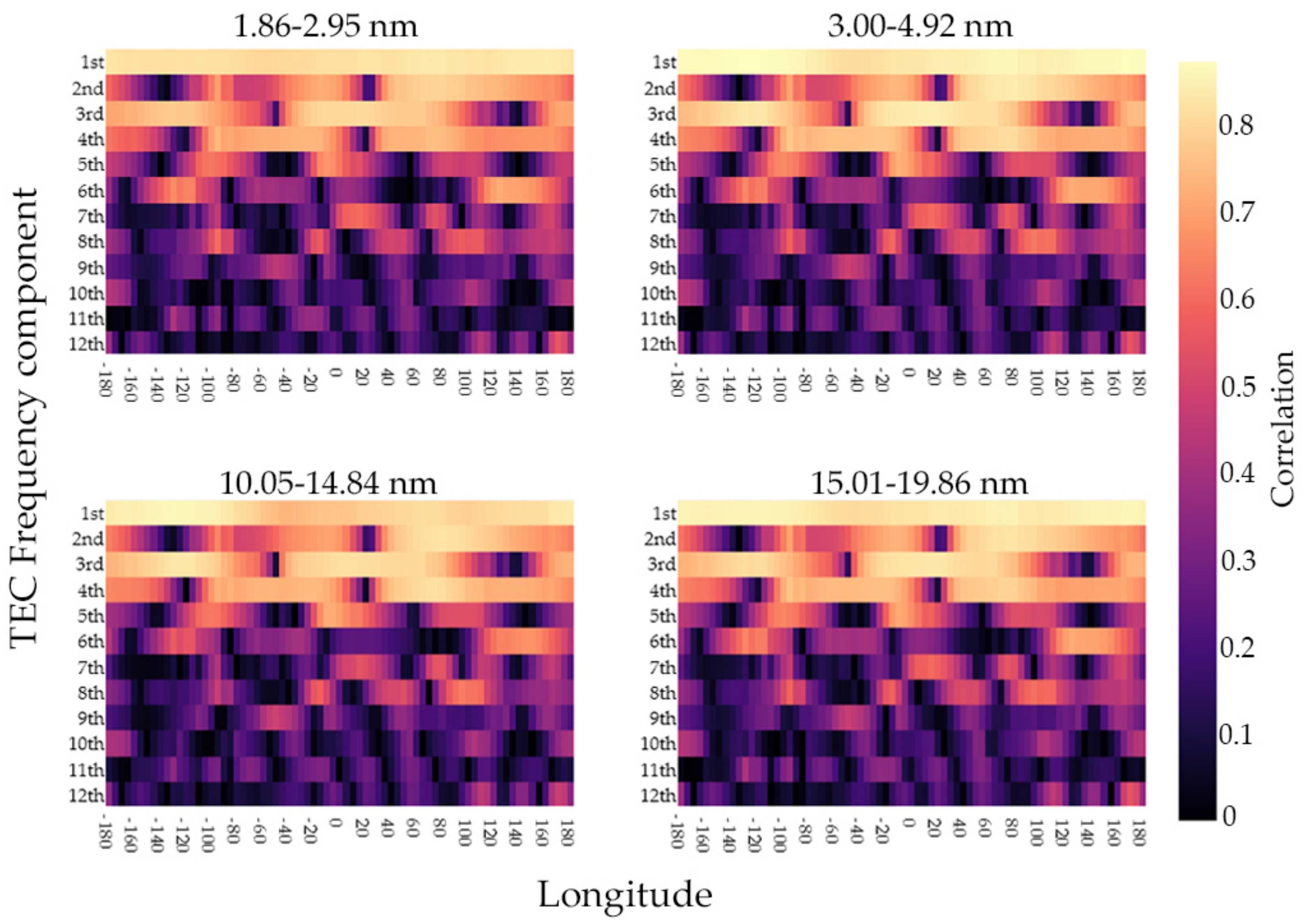
2.3. Photon Flux
3. Ionosphere Modeling
3.1. Linear Regression
3.2. Polynomial Regression
3.3. Support Vector Machine
3.4. Regularization Methods
4. Model Analysis and Experiments
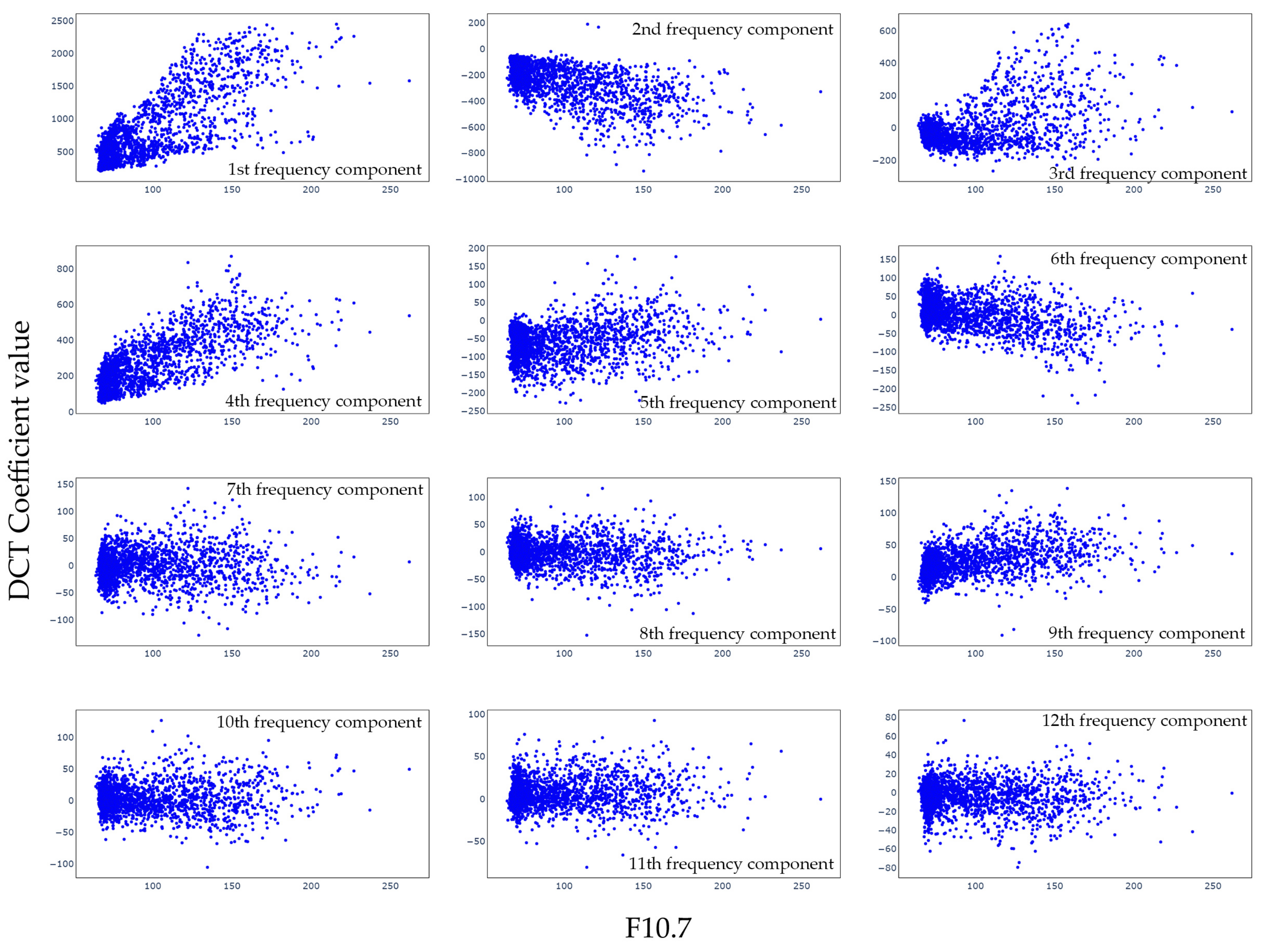
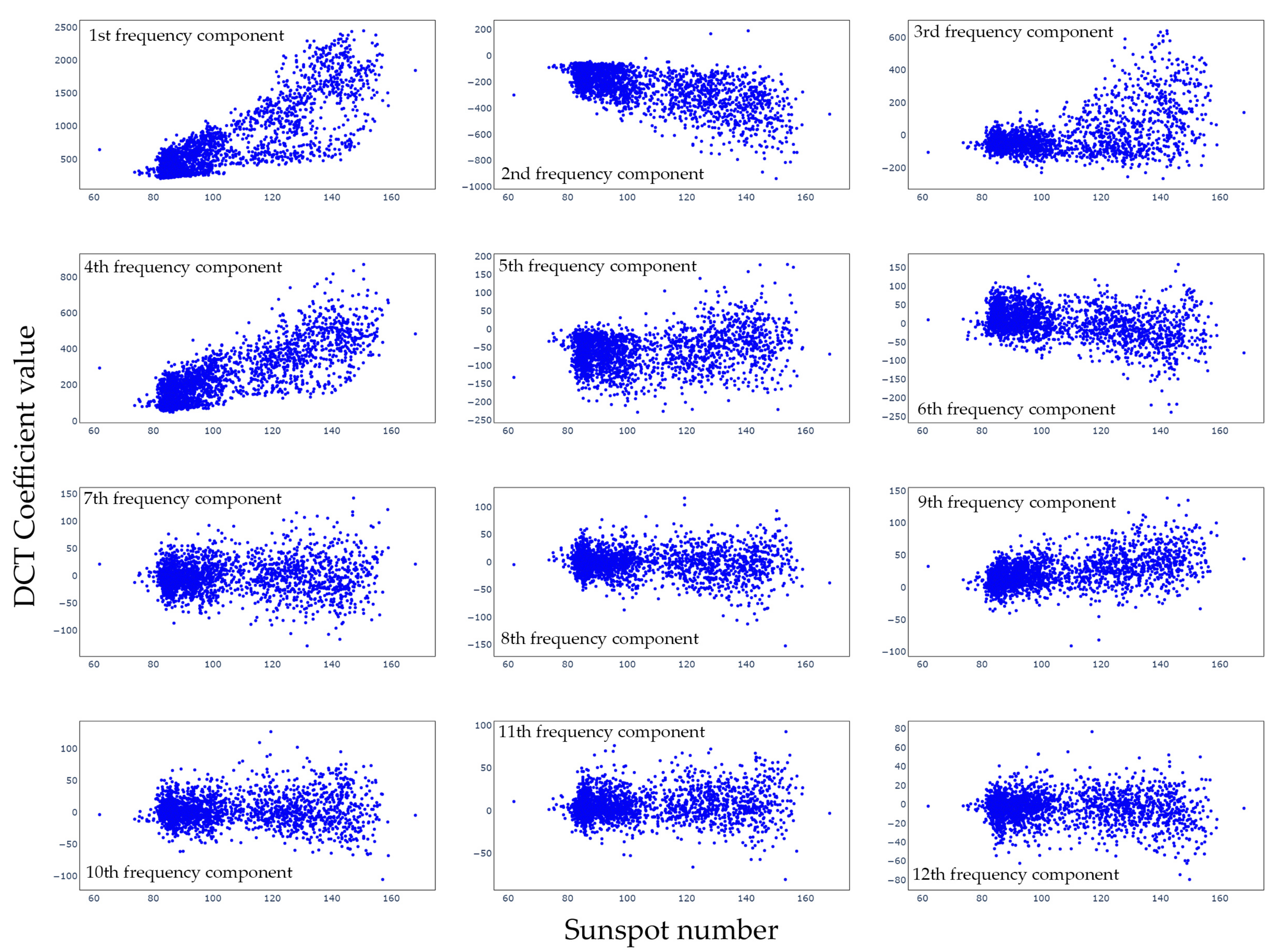
4.1. Features Correlation Analysis
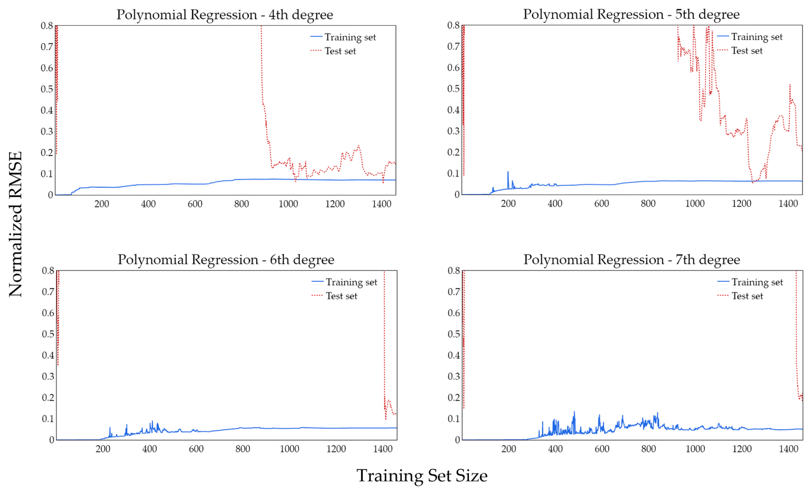
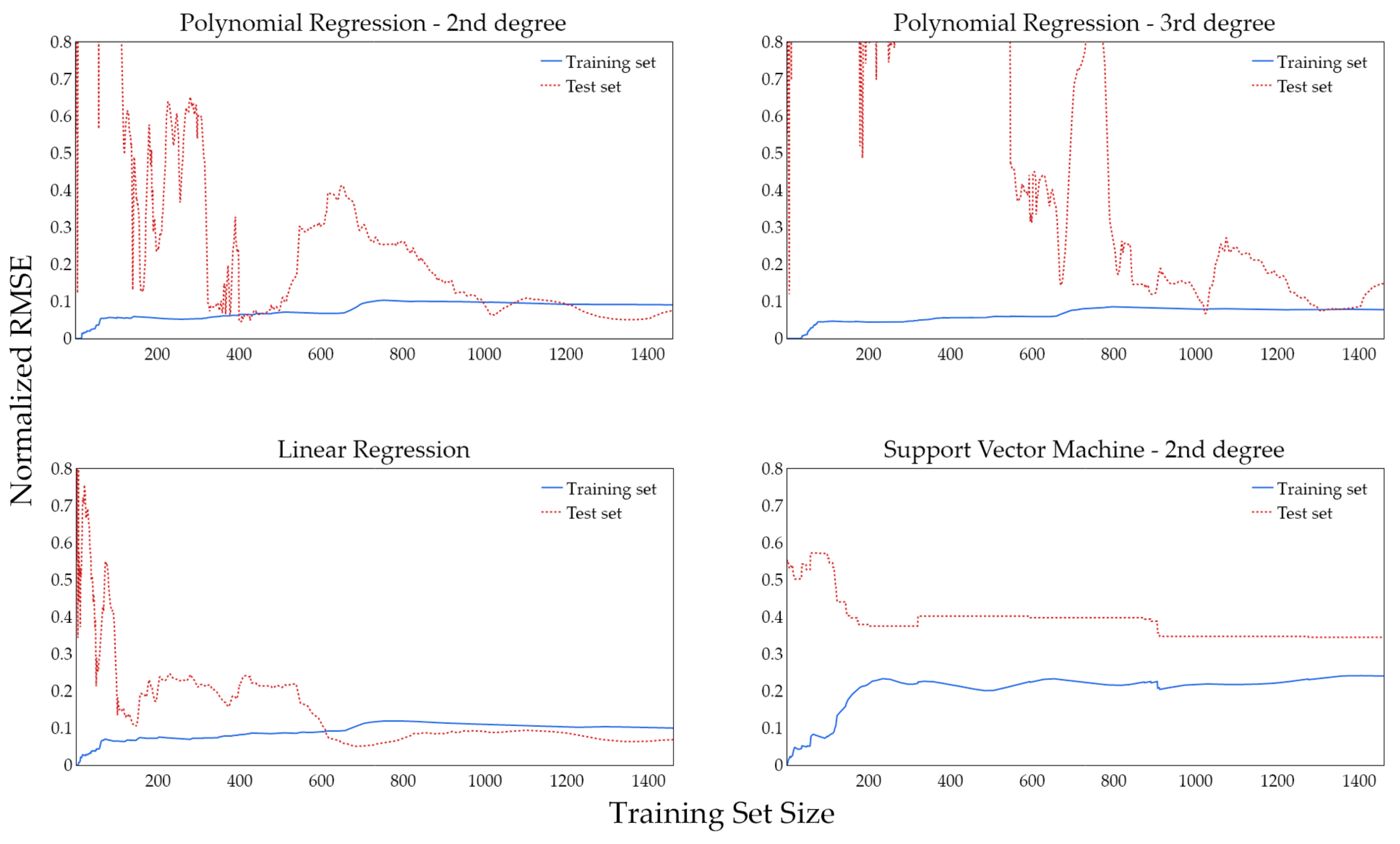
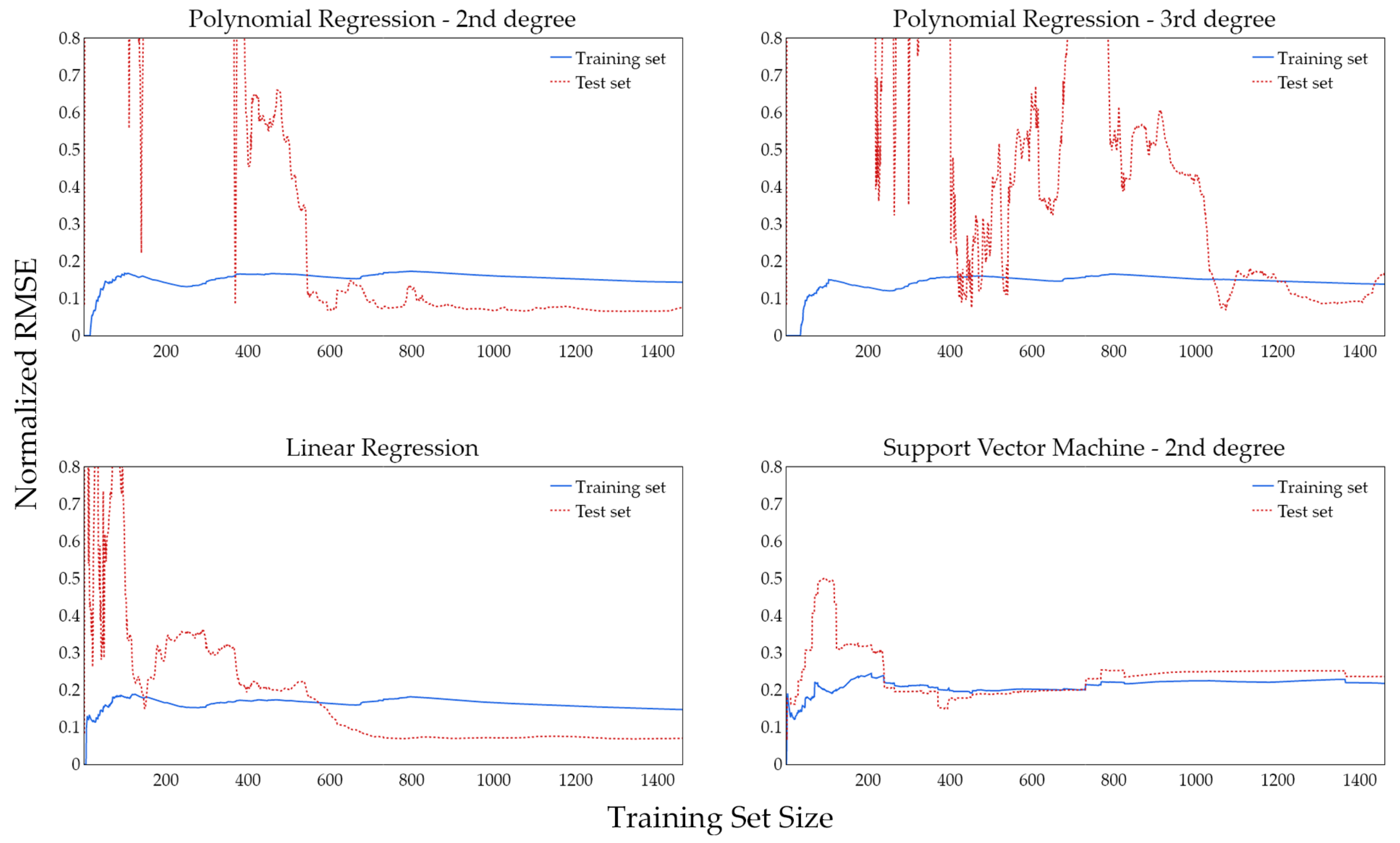
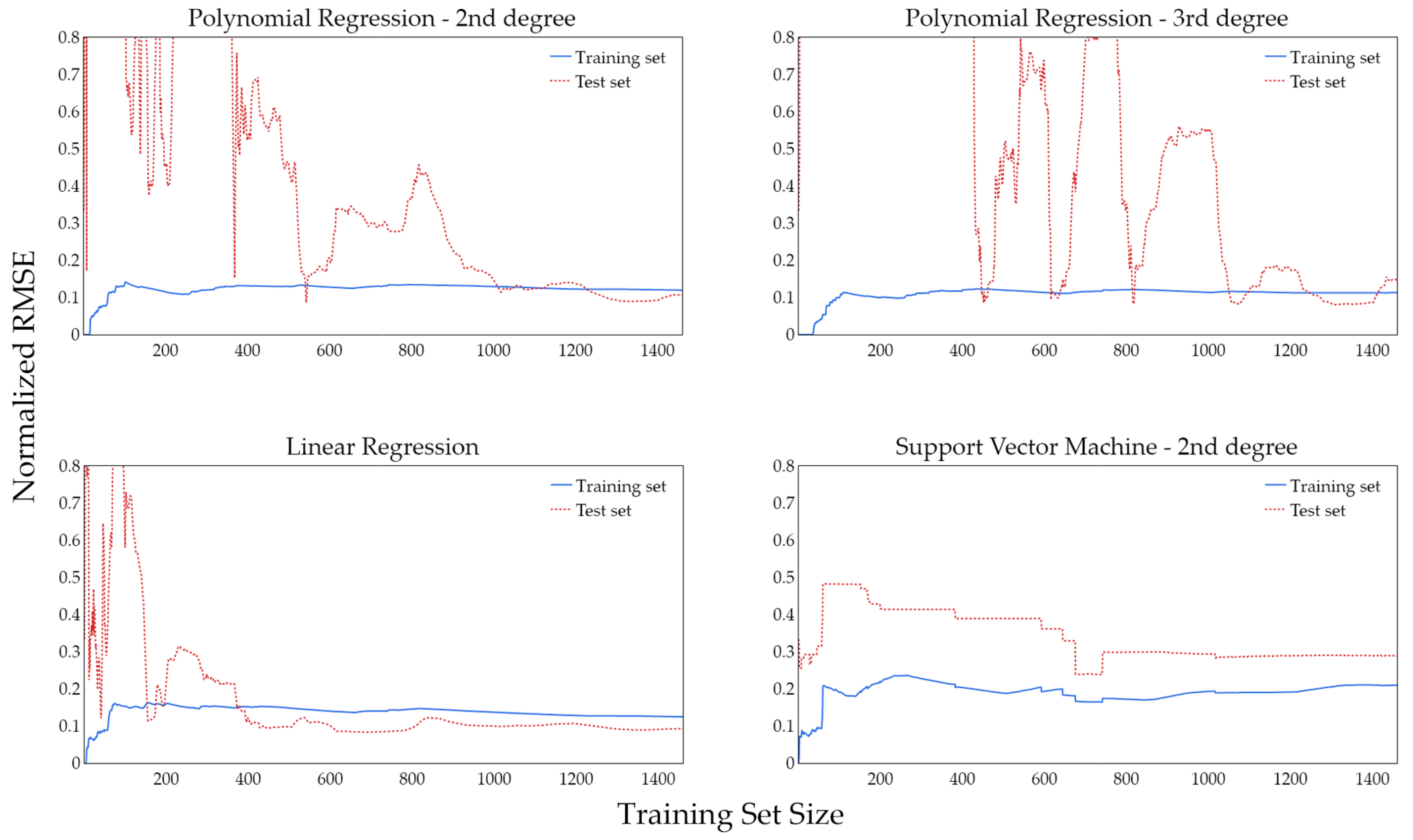
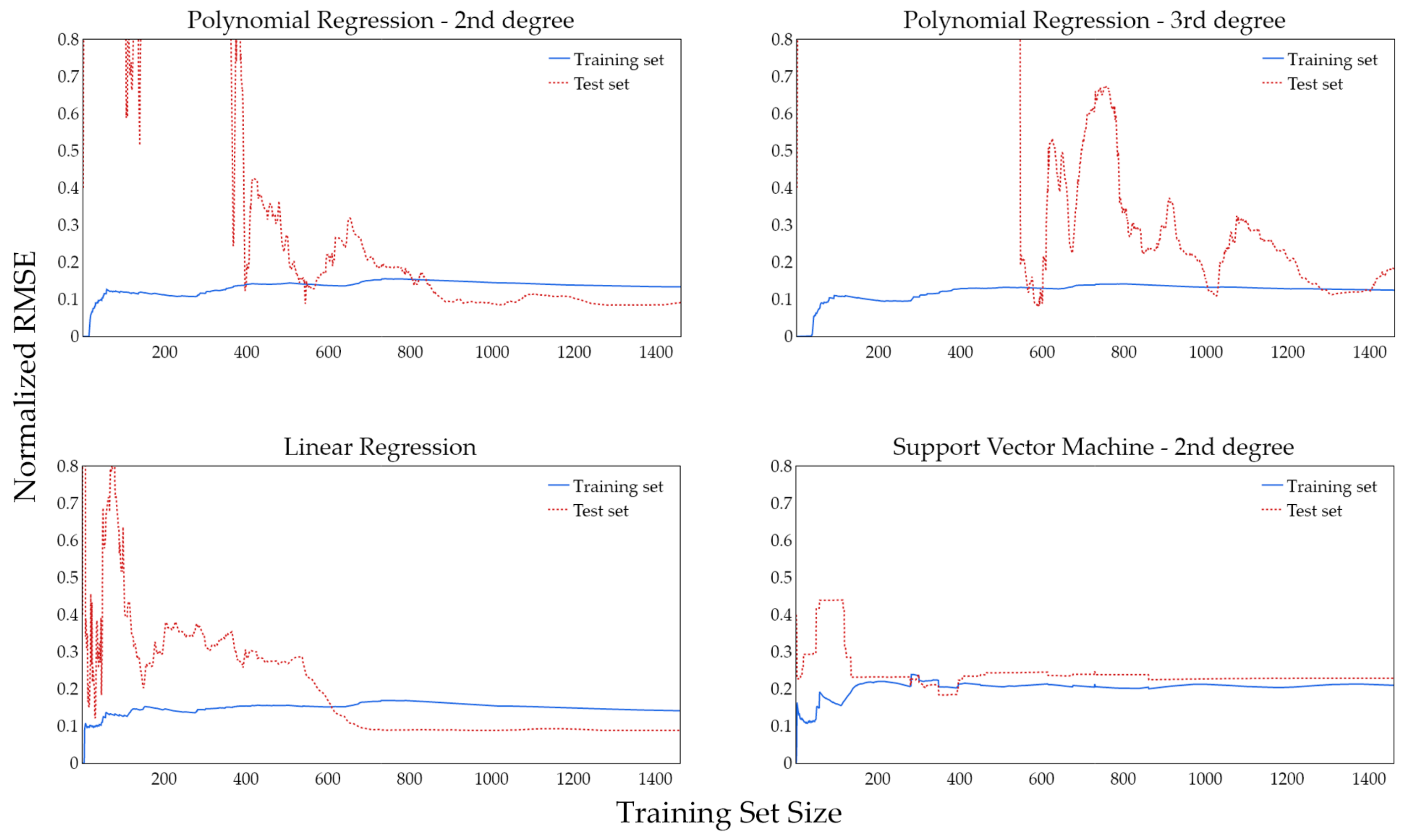
4.2. Learning Curves
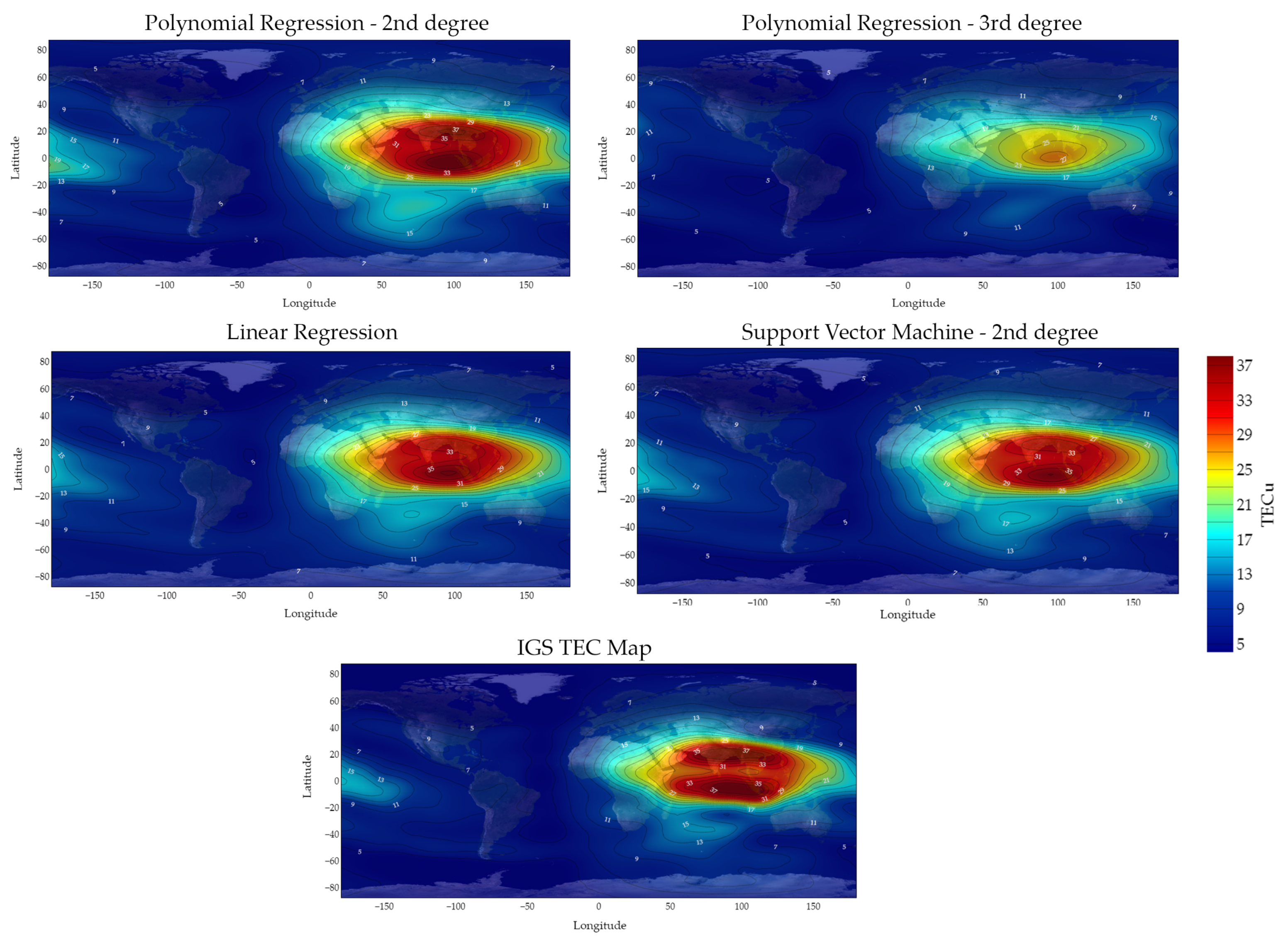
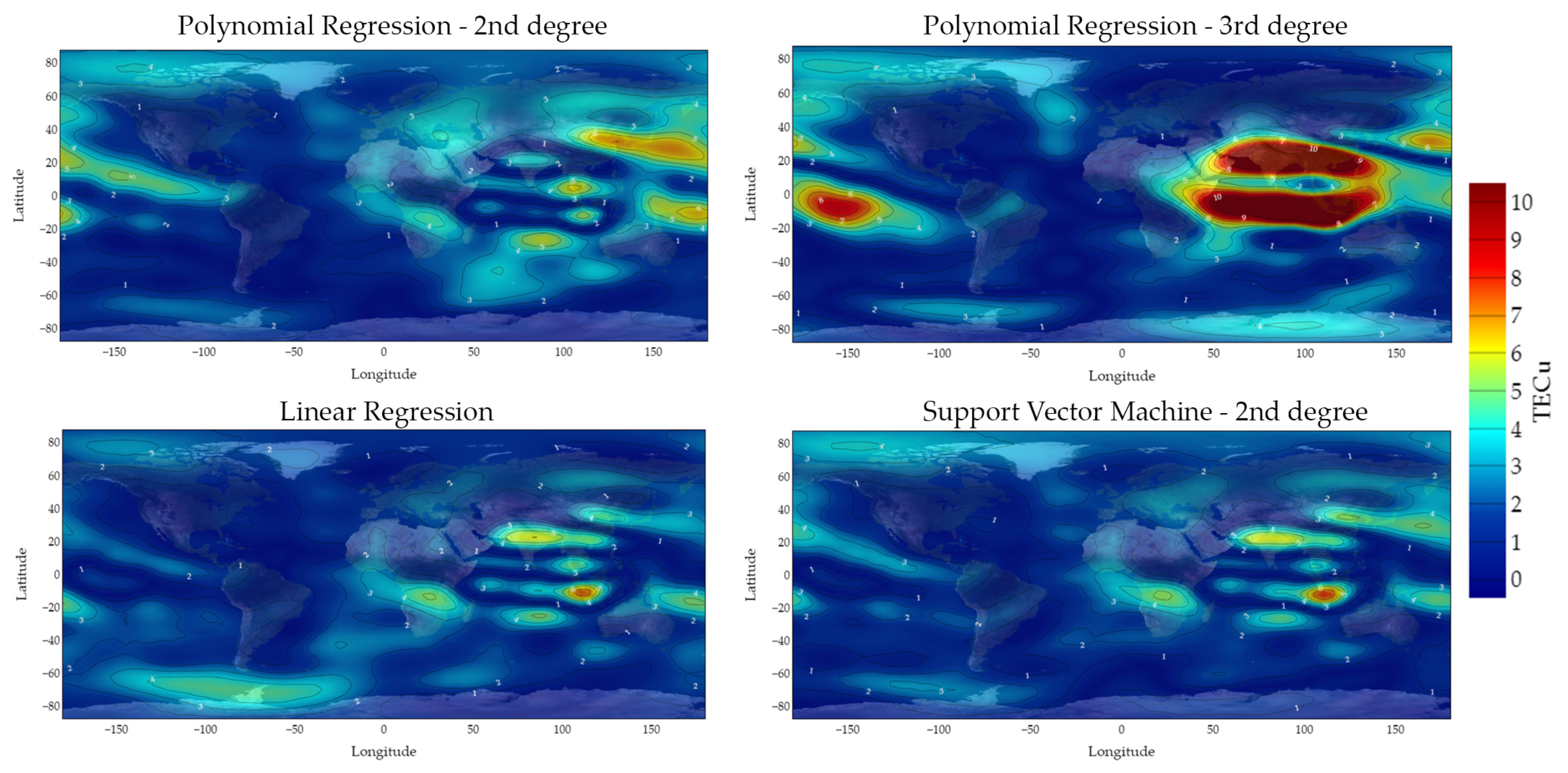
4.3. Reconstruction of TEC Maps
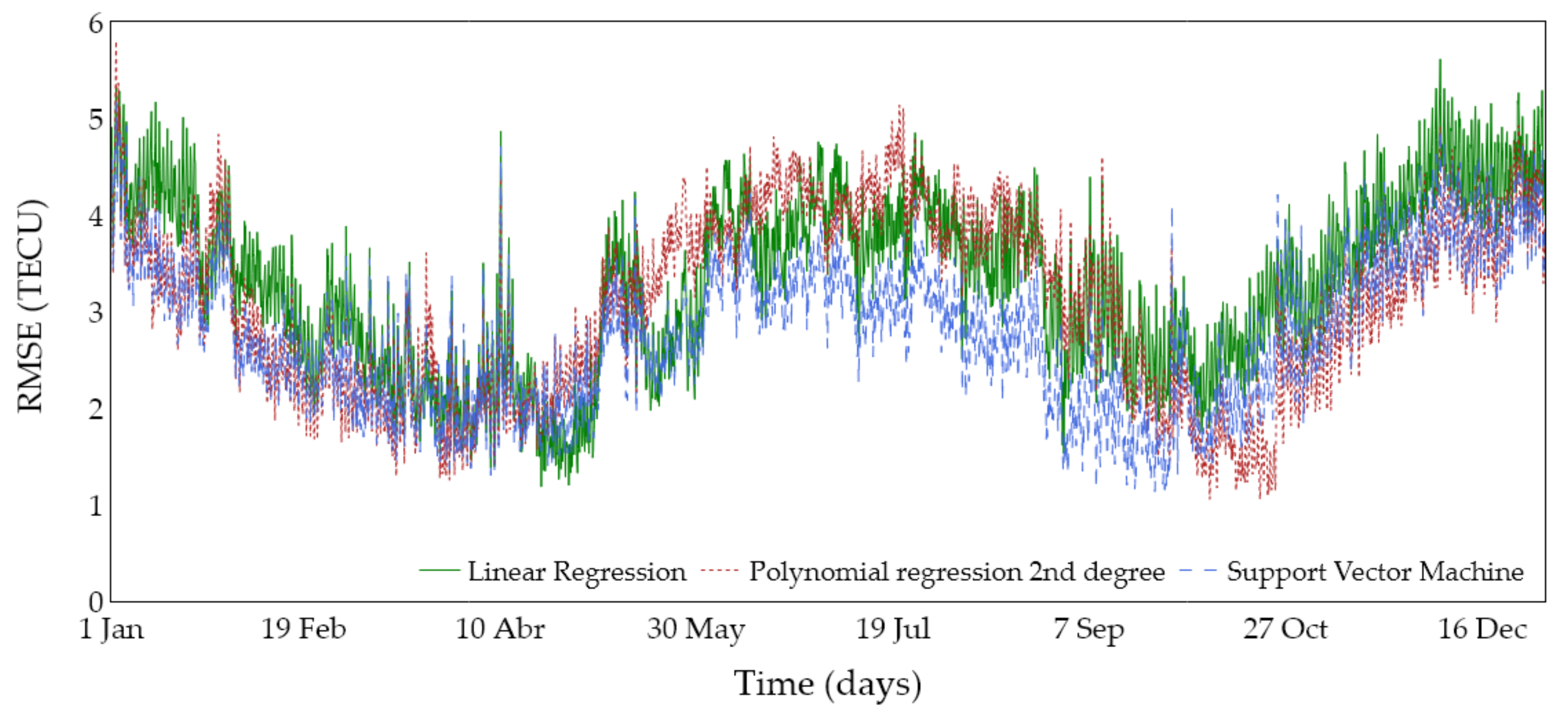
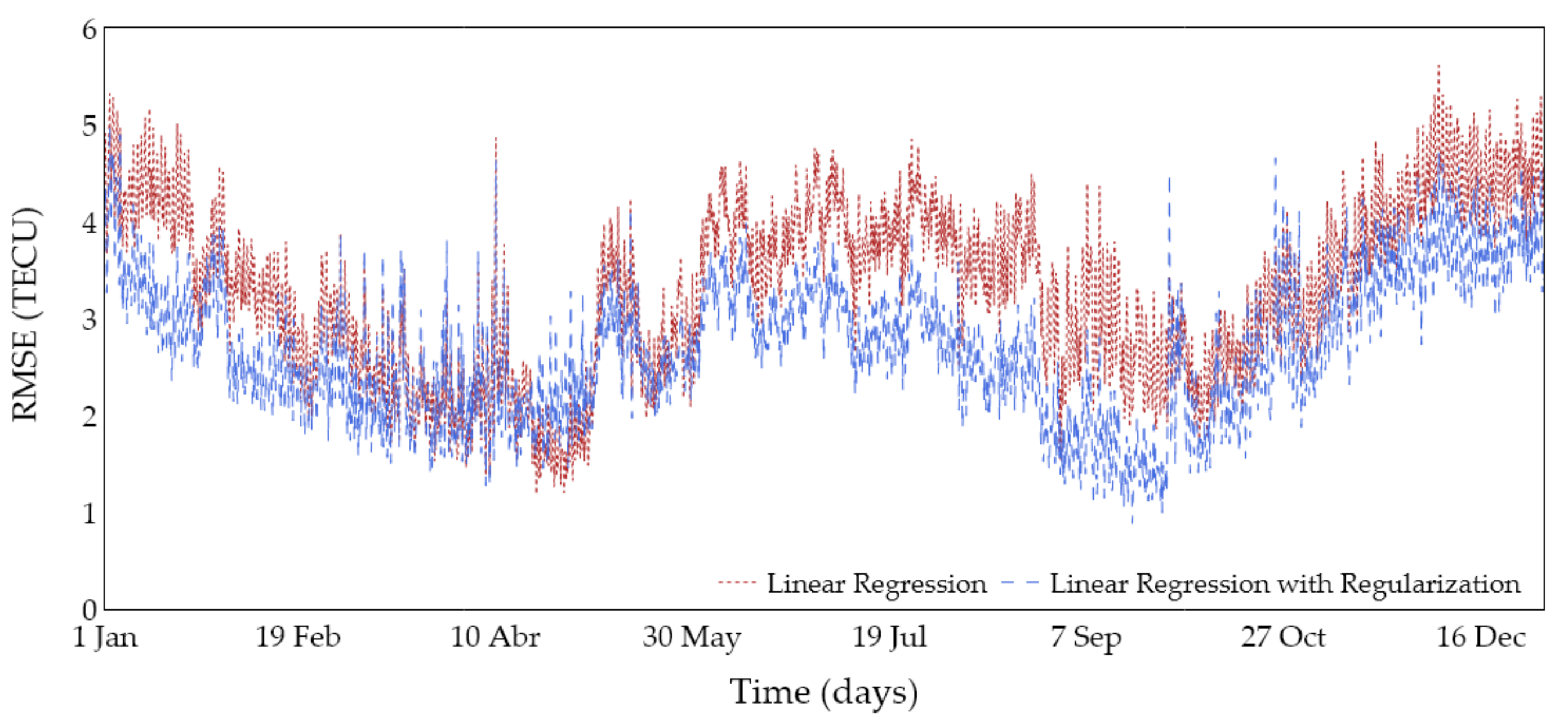
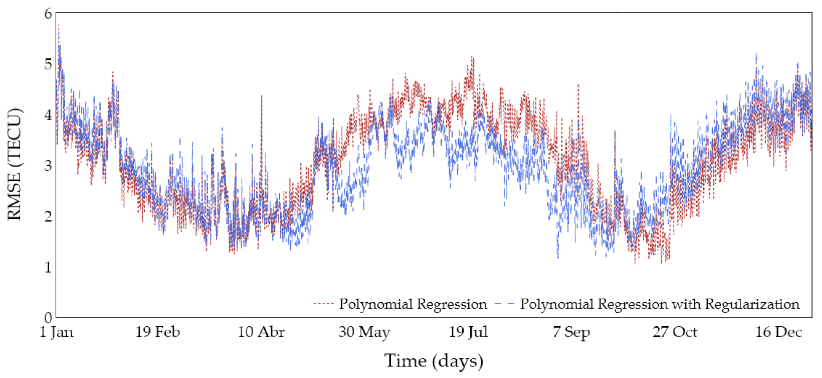
5. RMSE Results
Regularization
6. Conclusions and Future Work
Author Contributions
Funding
Institutional Review Board Statement
Informed Consent Statement
Data Availability Statement
Acknowledgments
Conflicts of Interest
Abbreviations
| TEC | Total Electron Content |
| GNSS | Global Navigation Satellite System |
| GPS | Global Positioning System |
| IGS | International GNSS Service |
| UTC | Coordinated Universal Time |
| DCT | Discret Cosine Transform |
| CME | Coronal Mass Ejection |
| RMSE | Root Mean Squared Error |
| NASA | National Aeronautics and Space Administration |
| SVM | Support Vector Machine |
| LASSO | Least Absolute Shrinkage and Selection Operator |
| MSE | Mean Squared Error |
References
- Moldwin, M. An Introduction to Space Weather, 3rd ed.; Cambridge University Press: New York, NY, USA, 2008; p. 156. [Google Scholar]
- GNSS Atmospheric Products—Ionosphere. Available online: https://cddis.nasa.gov/archive/gnss/products/ionex/ (accessed on 21 August 2020).
- Klobuchar, J.A. Ionospheric Time-Delay Algorithm for Single-Frequency GPS Users. IEEE Trans. Aerosp. Electron. Syst. 1987, AES-23, 325–331. [Google Scholar] [CrossRef]
- Bilitza, D.; Altadill, D.; Reinisch, B.; Galkin, I.; Shubin, V.; Truhlik, V. The International Reference Ionosphere: Model Update 2016. In Proceedings of the EGU General Assembly 2016, Vienna, Austria, 17–22 April 2016. [Google Scholar]
- Nava, B.; Coïsson, P.; Radicella, S.M. A new version of the NeQuick ionosphere electron density model. J. Atmos. Sol. Terr. Phys. 2008, 70, 1856–1862. [Google Scholar] [CrossRef]
- Jakowski, N.; Hoque, M.M.; Mayer, C. A new global TEC model for estimating transionospheric radio wave propagation errors. J. Geod. 2011, 85, 965–974. [Google Scholar] [CrossRef]
- Feng, J.; Han, B.; Zhao, Z.; Wang, Z. A New Global Total Electron Content Empirical Model. Remote Sens. 2019, 11, 706. [Google Scholar] [CrossRef] [Green Version]
- Géron, A. Hands-on Machine Learning with Scikit-Learn and Tensorflow, 2nd ed.; O’Reilly Media: Sebastopol, CA, USA, 2017; p. 549. [Google Scholar]
- Geryl, P.; Alvestad, J. A Formula for the Start of a New Sunspot Cycle; Springer: New York, NY, USA, 2020. [Google Scholar]
- Lin, C.H.; Liu, J.Y.; Fang, T.W.; Chang, P.Y.; Tsai, H.F.; Chen, C.H.; Hsiao, C.C. Motions of the equatorial ionization anomaly crests imaged by FORMOSAT-3/COSMIC. Geophys. Res. Lett. 2007, 34. [Google Scholar] [CrossRef]
- Xuguang, C.; Burns, G.A.; Wenbin, W.; Daniell, E.; Martinis, C.R.; McClintock, W.; Inez, S. Batista Observation of postsunset OI 135.6 nm radiance enhancement over South America by the GOLD mission. J. Geophys. Res. Space Phys. 2020, 126. [Google Scholar] [CrossRef]
- Gopalswamy, N. History and development of coronal mass ejections as a key player in solar terrestrial relationship. Geosci. Lett. 2016, 3, 8. [Google Scholar] [CrossRef] [Green Version]
- Chou, M.-Y.; Pedatella, N.M.; Wu, Q.; Huba, J.D.; Charles, C.H.L.; Schreiner, W.S.; Braun, J.J.; Eastes, R.; Yue, J. Observation and Simulation of the Development of Equatorial Plasma Bubbles: Post-Sunset Rise or Upwelling Growth? JGR Space Phys. 2020, 125, e2020JA028544. [Google Scholar]
- Karan, D.K.; Daniell, R.E.; England, S.L.; Martinis, C.R.; Richard, W.E.; Burns, G.A.; McClintock, W.E. First zonal drift velocity measurement of equatorial plasma bubbles (EPBs) from a geostationary orbit using GOLD data. J. Geophys. Res. Space Phys. 2020, 125, e2020JA028173. [Google Scholar] [CrossRef]
- Choudhuri, A.R. Nature’s Third Cycle, 3rd ed.; Oxford University Press: New York, NY, USA, 2015; p. 286. [Google Scholar]
- Tobiska, W.K.; Woods, T.; Eparvier, F.; Viereck, R.; Floyd, L.; Bouwer, D.; Rottman, G.; White, O.R. The SOLAR2000 empirical solar irradiance model and forecast tool. J. Atmos. Sol. Terr. Phys. 2000, 62, 1233–1250. [Google Scholar] [CrossRef]
- Rao, K.R.; Yip, P. Discrete Cosine Transform, Algorithms, Advantages, Applications, 1st ed.; Academic Press: Cambridge, MA, USA, 1990; p. 512. [Google Scholar]
- Hastie, T.; Tibshirani, R.; Friedman, J. The Element of Statistical Learning, Data Mining, Inference and Prediction, 2nd ed.; Springer Science+Business Media: New York, NY, USA, 2017; p. 446. [Google Scholar]
- Wasserman, L. All of Statistics, 1st ed.; Springer Science+Business Media: New York, NY, USA, 2004; p. 446. [Google Scholar]
- Hearst, A. Support vector machines. IEEE Intell. Syst. 1998, 13, 18–28. [Google Scholar] [CrossRef] [Green Version]
- Murphy, K. Machine Learning, a Probabilistic Perspective; MIT Press: Cambridge, MA, USA, 2012. [Google Scholar]
- Hastie, T.; Tibshirani, R.; Friedman, J. Statistics for High-Dimensional Data, 1st ed.; Springer Science+Business Media: New York, NY, USA, 2011; p. 575. [Google Scholar]
- Bogdan, M.; van den Berg, E.; Su, W.; Candès, E.J. Statistical Estimation and Testing via the Sorted L1 Norm; Departments of Mathematics and Computer Science, Wrocław University of Technology and Jan Długosz University: Częstochowa, Poland, 2013. [Google Scholar]
- Tibshirani, R. Regression Shrinkage and Selection via the Lasso. J. R. Stat. Soc. Ser. B (Methodol.) 1996, 58, 267–288. [Google Scholar] [CrossRef]


| Model | Global RMSE [TECU] |
|---|---|
| Linear Regression | 3.42 |
| Polynomial Regression (2nd degree) | 3.23 |
| Support Vector Machine | 2.89 |
| Model | Global RMSE (TECU) |
|---|---|
| Linear Regression with regularization | 2.80 |
| Polynomial Regression (2nd degree) with regularization | 3.07 |
Publisher’s Note: MDPI stays neutral with regard to jurisdictional claims in published maps and institutional affiliations. |
© 2021 by the authors. Licensee MDPI, Basel, Switzerland. This article is an open access article distributed under the terms and conditions of the Creative Commons Attribution (CC BY) license (https://creativecommons.org/licenses/by/4.0/).
Share and Cite
Benoit, A.G.M.d.S.; Petry, A. Evaluation of F10.7, Sunspot Number and Photon Flux Data for Ionosphere TEC Modeling and Prediction Using Machine Learning Techniques. Atmosphere 2021, 12, 1202. https://doi.org/10.3390/atmos12091202
Benoit AGMdS, Petry A. Evaluation of F10.7, Sunspot Number and Photon Flux Data for Ionosphere TEC Modeling and Prediction Using Machine Learning Techniques. Atmosphere. 2021; 12(9):1202. https://doi.org/10.3390/atmos12091202
Chicago/Turabian StyleBenoit, Andres Gilberto Machado da Silva, and Adriano Petry. 2021. "Evaluation of F10.7, Sunspot Number and Photon Flux Data for Ionosphere TEC Modeling and Prediction Using Machine Learning Techniques" Atmosphere 12, no. 9: 1202. https://doi.org/10.3390/atmos12091202