Spatiotemporal Analysis of Haze in Beijing Based on the Multi-Convolution Model

Abstract

As a kind of air pollution, haze has complex temporal and spatial characteristics. From the perspective of time, haze has different causes and levels of pollution in different seasons. From the perspective of space, the concentration of haze in adjacent areas will affect each other, showing some correlation. In this paper, we construct a multi-convolution haze-level prediction model for predicting haze levels in different areas of Beijing, which uses the remote sensing satellite image of the Beijing divided into nine regions as input and the haze pollution level as output. We categorize the predictions into four seasons in chronological order and use frequency histograms to analyze haze levels in different regions in different seasons. The results show that the haze pollution in the southern regions is significantly different from that in the northern regions. In addition, the haze tends to be clustered in adjacent areas. We use Global Moran’s I to analyze the predictions and find that haze is related to the geographical location in summer and autumn. We also use Local Moran’s I, Moran scatter plot, and Local Indicators of Spatial Association (LISA) to study the spatial characteristics of haze in adjacent areas. The results show, for the spatial distribution of haze in Beijing, that the southern regions present a high-high agglomeration, while the northern regions exhibit a ‘low-low agglomeration. The temporal evolution of haze on the seasonal scale, according to the chronological order of winter, spring, and summer to autumn, shows that the haze gradually becomes agglomerated. The main finding is that the haze pollution in southern Beijing is significantly different from that of northern regions, and haze tends to be clustered in adjacent areas.

1. Introduction

In recent years, haze has attracted the media’s attention, and that of the government and population of various countries. It has triggered a wide-ranging discussion on how to coordinate economic development and environmental protection. However, this started a public panic about air pollution and how this affected the physical health of people. Moreover, haze predicts human damage from air pollution [1,2]. For these reasons, haze has aroused the concern of researchers. Therefore, a large amount of experimental data and theoretical reasoning are focused on the cause of haze [3,4,5,6,7,8], the scope of pollution [9,10,11,12,13,14,15,16], the hazards [2,11,17,18,19,20,21,22], spatial and temporal distribution, and prevention measures.

With the establishment of many ground detection stations, the detection data of PM2.5 and PM10, which are the primary pollutants of haze, gradually increase, which facilitates the study of its spatial and temporal characteristics [8,14,15,20,22,23,24,25]. Researchers have performed analyses of the spatial and temporal evolution of haze in different areas based on satellite images [4,14,26,27,28]. Gehrig et al. [29] studied the long-term observations of PM2.5 and PM10 in seven regions of Switzerland and obtained the range of PM2.5 concentrations in different regions. Although there were different haze concentrations in different regions, the correlation between daily PM2.5 and PM10 concentrations was very high in all regions. In terms of time characteristics, the haze pollution in the Swiss region in winter is the most severe of the four seasons, and the haze pollution in the spring is the lightest. Zhang et al. [30] analyzed the PM2.5 concentration data of 190 cities in China. They found that the significant seasonal variation of PM2.5 occurred in winter and the lowest in summer on the time scale. In terms of the geographical distribution, the PM2.5 concentrations in the northern region are generally higher than in the south. Zhao et al. [27] collected PM2.5 and PM10 concentrations from 30 ground detection stations in Beijing and analyzed haze concentrations’ temporal and spatial distribution in winter and spring. The results showed that the concentration of haze in the northern mountains area is lower than that in the south of Beijing, and the haze pollution in urban and rural areas is quite different. The time characteristics of haze showed that there is serious pollution in winter and slight pollution in spring, the highest concentration of PM2.5 and PM10 appears in January, and the lowest concentration appears in April. Zhao et al. [31] compared the time characteristics of urban and rural areas in Beijing.

The concentration prediction of PM2.5 and PM10 as the primary pollutants of haze is also one of the most concerning areas, and researchers have proposed many different prediction models. In the early days of haze prediction, Fuller et al. [32] used empirical models to predict the daily average concentrations of PM2.5 and PM10 in some regions of the U.K., but the scalability was poor due to the model being based on observations in local areas. Dong et al. [33] proposed a hidden Markov-based prediction model to predict PM2.5 concentration. After training, the hidden Markov model can finally predict the PM2.5 concentration value in the next 24 h. Lee et al. [34] combined the MODIS aerosol optical depth (AOD) over England with ground monitoring data to predict haze concentrations in specific areas. As neural networks began to show solid complex-fitting capabilities, researchers began to apply different neural networks to predict haze. Ordieres et al. [35] compared the performance of three neural network structures—multilayer perceptron, radial basis function neural network, and squared multilayer perceptron—with classic predictive models in daily average PM2.5 concentration predictions. The neural networks are significantly better than the classic approaches. Marzano et al. [36] established a recurrent neural network to predict climate phenomena with input from remote sensing satellite imagery.

Unlike previous prediction models, which mainly predict PM2.5/PM10 concentration in a single area [37], this paper proposed a multi-convolution haze-level prediction model to simultaneously predict PM2.5 concentration levels in multiple adjacent areas. This paper used remote sensing satellite images from Beijing as the model’s input. The images are cut into nine blocks of the same size and applied in various data processing methods, including radiation correction, geometric correction, area extraction and synthesis, RGB image synthesis, and image cutting. This paper then uses the daily PM2.5 level of nine blocks as output.

In addition to predicting the haze levels in different blocks in Beijing, we also analyzed haze’s temporal and spatial characteristics in different areas. Previous researchers have focused on the temporal and spatial characteristics of haze in one area while ignoring the haze correlation between areas bordering each other. Therefore, this paper divided the predicted results into four seasons in chronological order and used frequency histograms to analyze the haze levels in different regions. Furthermore, this paper used the Global Moran’s I to obtain the correlation between haze in different seasons and geographic locations. It used the Local Moran’s I, Moran scatter plot, and Local Indicators of Spatial Association (LISA) to study the spatial characteristics of haze in adjacent regions.

2. Data Processing and Calibration

2.1. Remote Sensing Image Processing

In the haze spatial evolution, the haze in the immediate vicinity will be highly correlated to the appropriate length of time. In order to analyze the temporal and spatial evolution characteristics of haze, the input of the model needs to involve different regions. Therefore, we chose Beijing as the research object according to the administrative division. Beijing is the capital of China and has severe haze pollution [28]. There are 36 air pollutant monitoring stations relatively evenly distributed in different parts of Beijing, which provide us with historical haze concentration data for different regions [1]. Based on the available data from the ground stations, the time span is chosen as 2013 to 2015.

In this paper, we collect two types of dataset:

(1)

Real-time PM2.5 concentration was released by ground monitoring stations in Beijing in 2013 and 2014. The data in 2014 are converted into haze levels according to the correspondence table of haze concentration and haze level, which formed a training set of multi-convolution combined haze-level prediction models. The data in 2015 is also converted to haze levels to test model accuracy.

(2)

MOD02_1km data for the Beijing area in 2013 and 2014. The MOD02_1km data is a remote sensing satellite image containing latitude and longitude information in the Beijing area and is the model input.

We preprocess the remote sensing satellite images in Beijing to improve the model’s classification prediction accuracy and data consistency. We use ENVI 5.0 software (L3Harris Geospatial, Boulder, CO, USA) to process satellite images: radiation correction, geometric correction, area extraction and synthesis, RGB image synthesis, and image cutting.

(1)

Radiation correction. We use ENVI 5.0 to automate the radiation correction of MOD02_1km data.

(2)

Geometric correction. We use the MODIS data processing tool, Georeference MODIS in the ENVI software, to geometrically correct the data of the emissivity channel. In the calibration, we select the Beijing coordinate system in World Geodetic System 1984 (WGS-84) standard to geometrically correct the emissivity file and establish Ground Control Points (GCPS) as the standard for other channels to maintain consistent geometric correction results. Then we use GCPS generated by the emissivity to correct the reflectance file. After reading the GCPS, the Triangulation correction method and the Bilinear resampling method are selected so that the correction result of the reflectance can match the emissivity.

(3)

Area extraction and synthesis. According to the administrative area of Beijing: 39.4° N–41.1° N; 115.4° E–117.4° E, we cut the administrative regional geographic graphic files in ENVI software to obtain satellite images of the Beijing area. Next, we use the same method to cut the emissivity file and reflectivity file of the satellite image, then place the file of the emissivity channel on the top, and the reflectivity channel file on the bottom. Finally, we synthesize the image to obtain the full channel satellite image with the same administrative scope and uniform size.

(4)

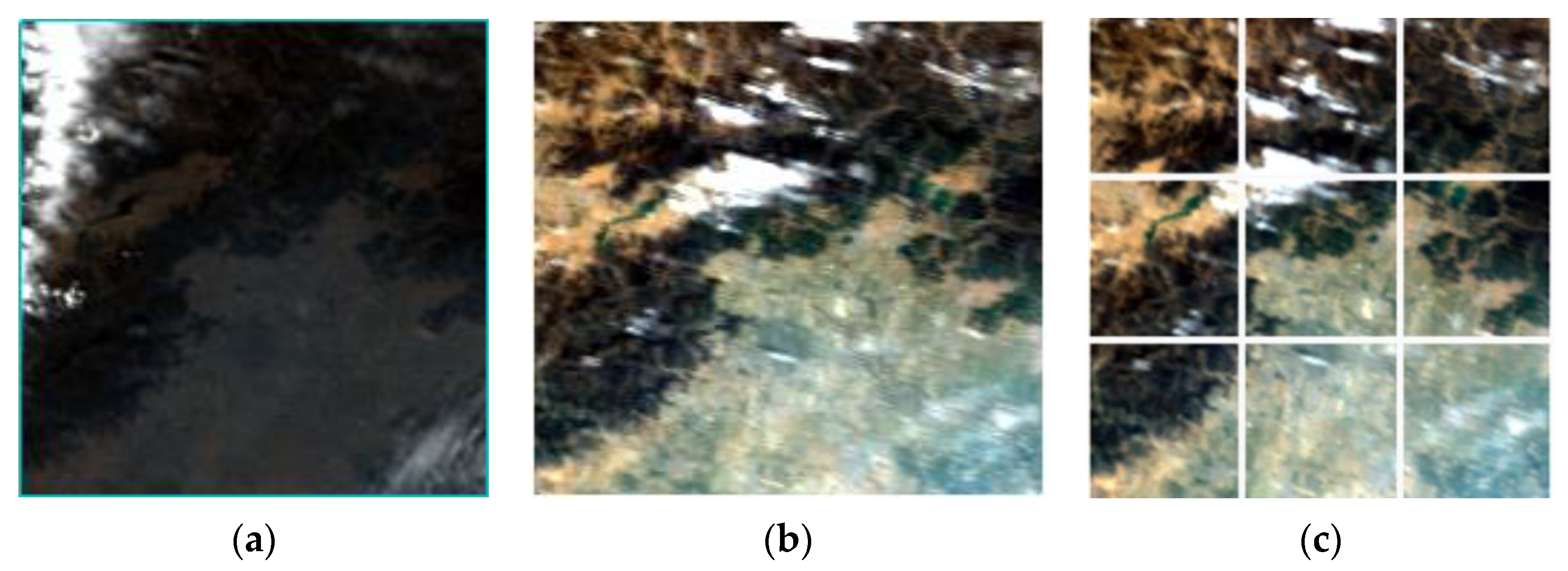
RGB image synthesis. The processed satellite image contains multiple channels, where channels 1–7 monitor the edge of the land and cloud. The wavelength and spatial resolution of each channel are shown in Table 1. We want to convert satellite images into three-channel RGB images by combining multiple suitable channels. The wavelength range of red light is between 622 and 780; green light is between 492 and 577; blue light is between 455 and 470. Comparing the visible light and satellite channel information, we synthesize the satellite’s channel 1, channel 4, and channel 3, and the synthesized results are shown in Figure 1a,b.

(5)

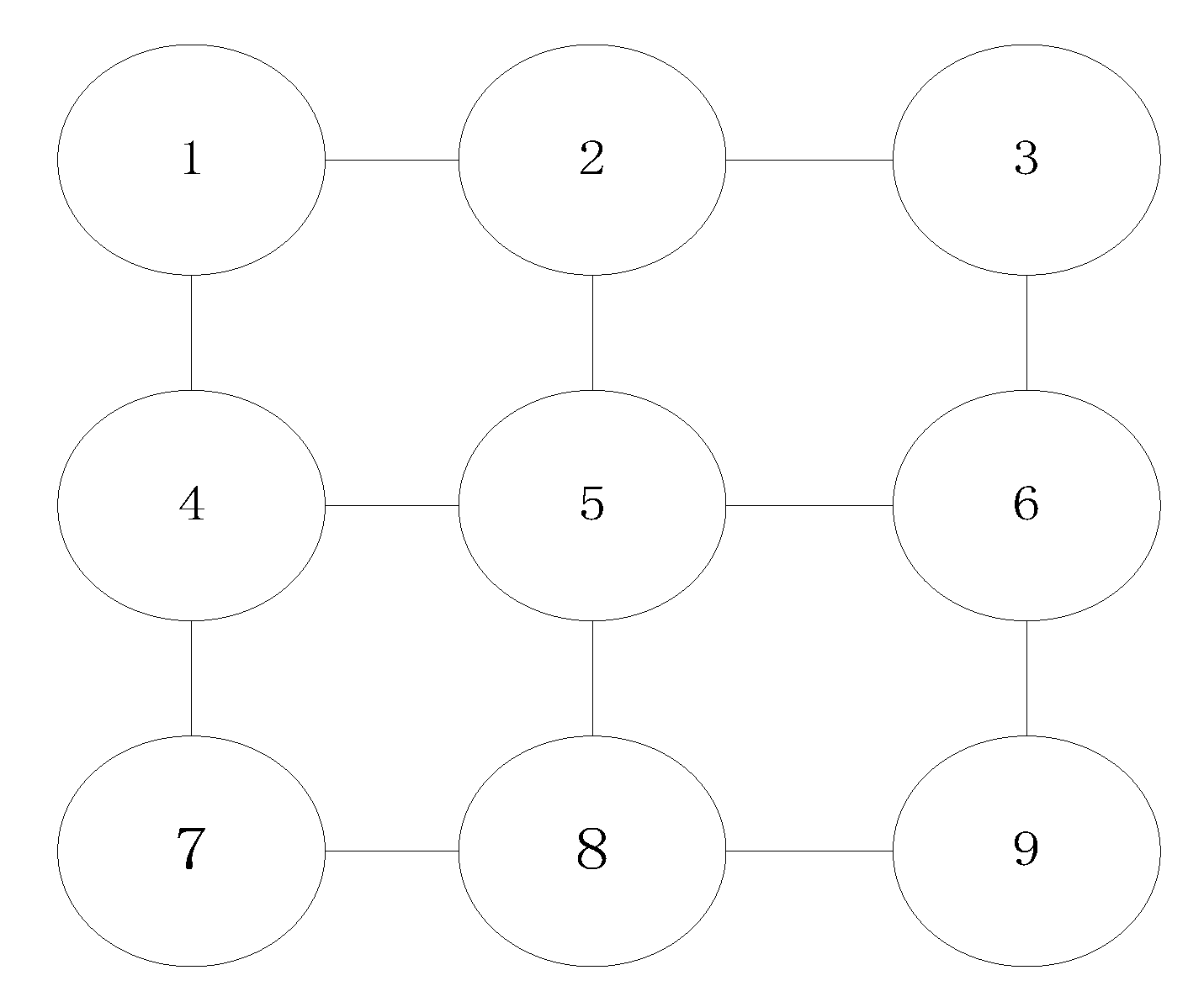
Image cutting: We cut the satellite image into nine equally sized blocks, as shown in Figure 1c. Every block of the image contains an actual region of Beijing. Thus, different blocks are adjacent from spatial relationships, which helps us study the haze’s spatial evolution.

After the synthesized RGB satellite image Figure 1b is cut, Figure 1c contains nine blocks of the same size, and we sort them from left to right and from top to bottom in Block 1 to Block 9. The administrative divisions contained in different blocks are shown in Table 2.

Figure 1. (a) is the satellite image with full channel information, and (b) is the synthesized RGB image. (c) is cut into nine equally sized blocks based on (b).

Figure 1. (a) is the satellite image with full channel information, and (b) is the synthesized RGB image. (c) is cut into nine equally sized blocks based on (b).

Table 1. Spatial resolution and wavelength interval of each channel in MOD021KM.

Channel	Wavelength Interval (nm)	Spatial Resolution (m)
1	620–670	250
2	841–876	250
3	459–479	500
4	545–565	500
5	1230–1250	500
6	1628–1652	500
7	2105–2155	500

Table 1. Spatial resolution and wavelength interval of each channel in MOD021KM.

Channel	Wavelength Interval (nm)	Spatial Resolution (m)
1	620–670	250
2	841–876	250
3	459–479	500
4	545–565	500
5	1230–1250	500
6	1628–1652	500
7	2105–2155	500

Table 2. Correspondence between block and administrative divisions.

Block	Administrative Divisions
1	Yanqing
2	Huairou
3	Miyun
4	Changping + Haidian (Metropolitan Area)
5	Shunyi + Chaoyang (Metropolitan Area)
6	Pinggu
7	Mentougou + Fangshan
8	Metropolitan Area + Daxing
9	Tongzhou

Table 2. Correspondence between block and administrative divisions.

Block	Administrative Divisions
1	Yanqing
2	Huairou
3	Miyun
4	Changping + Haidian (Metropolitan Area)
5	Shunyi + Chaoyang (Metropolitan Area)
6	Pinggu
7	Mentougou + Fangshan
8	Metropolitan Area + Daxing
9	Tongzhou

2.2. Haze Level Transformation

The haze-level prediction model outputs haze levels in different regions. Therefore, we divide the collected PM2.5 concentration in Beijing into 10 levels. Level 1: 0–35 μg/m³, air quality is good, basically no pollution; level 2: 36–70 μg/m³, acceptable; level 3: 71–105 μg/m³, mild pollution; level 4: 106–140 μg/m³, moderate pollution; level 5–7: 141–245 μg/m³, severe pollution; level 8–10: 245–500 μg/m³, severe pollution. We use the one-hot vector to label the training set, as in (1).

$$y_i=\left[p,c_1,c_2,\dots c_n\right]$$

(1)

The p-bit of the first element in the vector indicates whether there is a cloud layer effect and whether haze characteristics can be extracted. If p = 1, it means that haze characteristics are undetectable. In this case, the parameter optimization is to ignore the subsequent elements so that the adjustment of the parameters will not be affected in training; if p = 0, it means that the haze characteristics can be detected. When n represents the number of haze level, the subsequent c_n represent the corresponding haze level. If the number of c₄ is 1, it indicates the corresponding haze level of the input data is 4. i indicates the serial number of the region where the PM2.5 concentration is located, and i ranges from 1 to 9. Hence, the ground truth corresponding to each satellite image is as shown in (2).

$$y=\left[\begin{array}{ccccccccc}{p}^1& c_1^1& \dots & c_{10}^1& \dots & p^9& c_1^9& \dots & c_{10}^9\end{array}\right]$$

(2)

3. Method

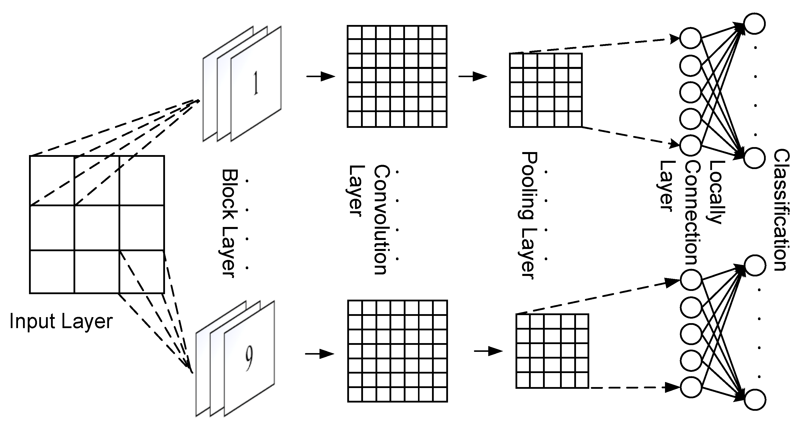
3.1. Joint Structure of Multi-Convolution Neural Networks

In order to identify haze grades for finer spatial scales and study the temporal and spatial evolution of haze in different regions of Beijing, we use a multi-convolution network structure to segment the haze data and then classify it. The multi-convolution neural network structure includes an input layer, block layer, convolution layer, pooling layer, local full connection layer, and classification layer [37], as shown in Figure 2. In this network, we use unified input and unified output.

The input layer accepts the processed satellite images in the Section 2 as inputs to obtain more spatio-temporal data.

The block layer is a sliding window, whose size is 60 × 60 × 3. The sliding step is 60, so the original 180 × 180 × 3 images can be divided into 9 blocks from the upper to the lower, from left to right, and then input into the different convolution neural networks.

Nine convolution layers acquire image features of nine different regions. Because different regions have different background information, such as geographical environment, the separated convolution layer can distinguish the fine-grained differences of different regions and provide the haze levels of different regions.

The pooling layer can help reduce the size of the model and increase the speed of the operation. First, we set padding with 0 and choose the maximum pooling function. Max pooling uses the maximum value of the region to replace all the elements in the region.

The locally full connection layer prevents cross-contamination of the different layer outputs at the fully connected layer, preserving the characteristics of each region. Each locally full connection corresponds to a soft-max classification layer. The classification layer consists of 99 nodes corresponding to nine regions. The marking and representation of data is the same as in Equation (2).

3.2. Spatial Autocorrelation Analysis of Haze Concentration

Global spatial autocorrelation analysis can reflect the relationship between haze concentration and spatial distribution. Suppose a piece of data is related to geographic location. In that case, the distribution of the data in geographic space is also correlated, and the degree of correlation is inversely proportional to the region’s distance. Its distribution methods are clustering, random distribution, and regular distribution. Through the spatial autocorrelation analysis of haze, this phenomenon can be better understood. Its essence is to analyze haze distribution in different geographic spaces and the correlation between different regions. In this section, the specific forms of using the matrix notation method to mark the data of the nine blocks are from top to bottom, and from left to right are Block 1 to Block 9.

3.2.1. Global Moran’s I

We use the Global Moran’s I to study the overall spatial characteristics of haze, indicating whether the haze is related to space, as in (3).

$$I=\frac{n{\sum }_{i=1}^n{\sum }_{j=1}^n{w}_{ij}\left(p_i-\overline{p}\right)\left(p_j-\overline{p}\right)}{{\sum }_{i=1}^n{\sum }_{j=1}^n{w}_{ij}·{\sum }_{i=1}^n{(p_i-\overline{p})}^2}$$

(3)

This paper cuts the satellite image into nine sub-regions of the same size, so n = 9 in the Equation. $p_i,p_j$ denote the average levels for Block i and Block j in one of the seasons. $\overline{p}$ denotes the average haze level for all blocks in a given season.$w_{ij}$ represents the weight between Block i and Block j. Since the image is equally divided, the areas on the diagonal are not considered to be adjacent. Then its spatial adjacency graph is as shown in Figure 3 below:

From the adjacency relationship in the above figure, we can obtain its spatial adjacency matrix, the weight matrix in this section. We set each side to be 1, and the weight between two blocks is 1, as in Equation (4), and the weight matrix is as shown in Equation (5).

$$w_{ij}=\{\begin{array}{l}1 \mathrm{if} \mathrm{Block} i \mathrm{is} \mathrm{adjacent} \mathrm{to} \mathrm{Block} j\\ 0 \mathrm{other}\end{array}$$

(4)

$$W=\left[\begin{array}{ccc}\begin{array}{ccc}0& 1& 0\\ 1& 0& 1\\ 0& 1& 0\end{array}& \begin{array}{ccc}1& 0& 0\\ 0& 1& 0\\ 0& 0& 1\end{array}& \begin{array}{ccc}0& 0& 0\\ 0& 0& 0\\ 0& 0& 0\end{array}\\ \begin{array}{ccc}1& 0& 0\\ 0& 1& 0\\ 0& 0& 1\end{array}& \begin{array}{ccc}0& 1& 0\\ 1& 0& 1\\ 0& 1& 0\end{array}& \begin{array}{ccc}1& 0& 0\\ 0& 1& 0\\ 0& 0& 1\end{array}\\ \begin{array}{ccc}0& 0& 0\\ 0& 0& 0\\ 0& 0& 0\end{array}& \begin{array}{ccc}1& 0& 0\\ 0& 1& 0\\ 0& 0& 1\end{array}& \begin{array}{ccc}0& 1& 0\\ 1& 0& 1\\ 0& 1& 0\end{array}\end{array}\right]$$

(5)

In this section, the essential reason for using the Moran’s I is to analyze and indirectly reflect the correlation between the two spatially adjacent areas of the haze concentration level. In order to facilitate the analysis and use of the Moran’s I, we use (6)–(8) to simplify (3).

$$S_0={{\displaystyle \sum }}_{i=1}^n{{\displaystyle \sum }}_{j=1}^n{w}_{ij}$$

(6)

$$z_i=\left(p_i-\overline{p}\right)$$

(7)

$$z^T=\left[z_1,z_2,\dots ,z_n\right]$$

(8)

The simplified global Moran’s I is given by (9).

$$I=\frac{n}{S_0}\frac{{\sum }_{i=1}^n{\sum }_{j=1}^n{w}_{ij}{z}_i{z}_j}{{\sum }_{i=1}^n{z}_i^2}=\frac{n}{S_0}\frac{z^{T}Wz}{z^{T}z}$$

(9)

The range of the global Moran’s I is between [−1, 1]. If I > 0, the haze has a positive correlation with the space and, the closer the value is to 1, the stronger the correlation, and there is a strong positive correlation between haze and space. Conversely, if I < 0, the haze is negatively correlated with space, and the closer the value is to −1, the stronger the negative correlation.

The analysis methods of spatial autocorrelation generally consist of the following three types: 1. Local Indicators of Spatial Association (LISA); 2. G statistics; 3. Moran scatter plot; the first is the method of local spatial analysis, which will be used in the following experiment. In the global analysis, the Moran scatter diagram is adopted as the analysis method, and its four quadrants respectively represent the spatial relationship between the four blocks and their neighboring blocks, and the corresponding relationships are as follows:

As shown in Figure 4, the Moran scatter plot consists of four quadrants representing four different spatial association types. The relationship of the first quadrant is high–high, indicating that the haze concentration level of the area and the surrounding area are both high, and the spatial difference is slight. The spatial relationship is a positive correlation. The relationship of the second quadrant is low–high, indicating that the haze level of the area and the surrounding area differs significantly. The level of the area is low, and the haze level around it is high. The spatial relationship is now negatively correlated. The relationship of the third quadrant is low–low, indicating the haze concentration in this area is low, and the spatial relationship is positive. The relationship between the fourth quadrant is high–low, indicating that the haze level in the area is high. However, the haze concentration level in the surrounding area is low. The spatial relationship is negatively correlated. Quadrant 1 and quadrant 3 reveal positive local spatial autocorrelation, and quadrant 2 and quadrant 4 reveal negative local spatial autocorrelation.

3.2.2. Local Moran’s I

Like the global Moran’s I, the local Moran’s I focuses on a specific block to describe the similarity between Block i and its adjacent areas, as shown in (10).

$$I_i=\frac{n\left(p_i-\overline{p}\right){\sum }_{j=1}^n{w}_{i,j}\left(p_j-\overline{p}\right)}{{\sum }_{i=1}^n{(p_i-\overline{p})}^2}=\frac{n{z}_i{\sum }_{j=1}^n{w}_{i,j}{z}_j}{z^{T}z}$$

(10)

The standardized statistics for local Moran’s I monitoring are specified in the following form:

$$Z\left(I_i\right)=\frac{I_i-E\left(I_i\right)}{\sqrt{Var\left(I_i\right)}}$$

(11)

This formula can be used to study the spatial heterogeneity of each region, and can also study and analyze the relative spatial relationship and its changes, where $E\left(I_i\right)$ represents the mathematical expectation of the Local Moran’s I of the i-th Block under the condition of no spatial autocorrelation, and its formula is expressed as:

$$E\left(I\right)=-\frac{1}{n-1}$$

(12)

$\sqrt{Var\left(I_i\right)}$ represents the standard deviation of the Local Moran’s I in the region. Since the LISA method is relatively intuitive, in the local analysis the Local Moran’s I of LISA is used for spatial analysis.

By comparing the sign of $Z\left(I_i\right)$ and the value of the local correlation coefficient $I_i$, the spatial units whose local correlation index reaches a certain threshold can be divided into four types of spatial autocorrelation relationships, as shown in the following

Table 3. Corresponding values of time–space relationship.

${\mathit{I}}_{\mathit{i}}$	$\mathit{Z}\left({\mathit{I}}_{\mathit{i}}\right)<0$	$\mathit{Z}\left({\mathit{I}}_{\mathit{i}}\right)>0$
Positive	low-high	high-high
negative	low-low	high-low

.

Among these, the local Moran’s I, whose significance level reaches a certain threshold, indicates a positive correlation in the spatial relationship. If it is significantly negative, it indicates a negative correlation between the two research areas in the space–time relationship. Combined with the standardized measurement Z, the time–space relationship can be analyzed. The high–high type indicates that the haze density level of area i and its neighboring blocks are relatively high. This area is a point where haze occurs frequently. The low–low type indicates that the haze concentration levels of the research block i and the surrounding adjacent blocks are relatively low. It indicates an area with lighter haze pollution. The other two types, low–high and high–low respectively, indicate that the high-pollution area surrounds the polluted area, and the high-pollution area is surrounded by the low-pollution area, showing a negative correlation. Compared with the spatial analysis obtained by general actual monitoring sites, the research in this section has the advantage that the research areas are distributed in equal blocks in time and space, and the distances are equal. Therefore, the accuracy of the weight matrix is higher.

4. Results

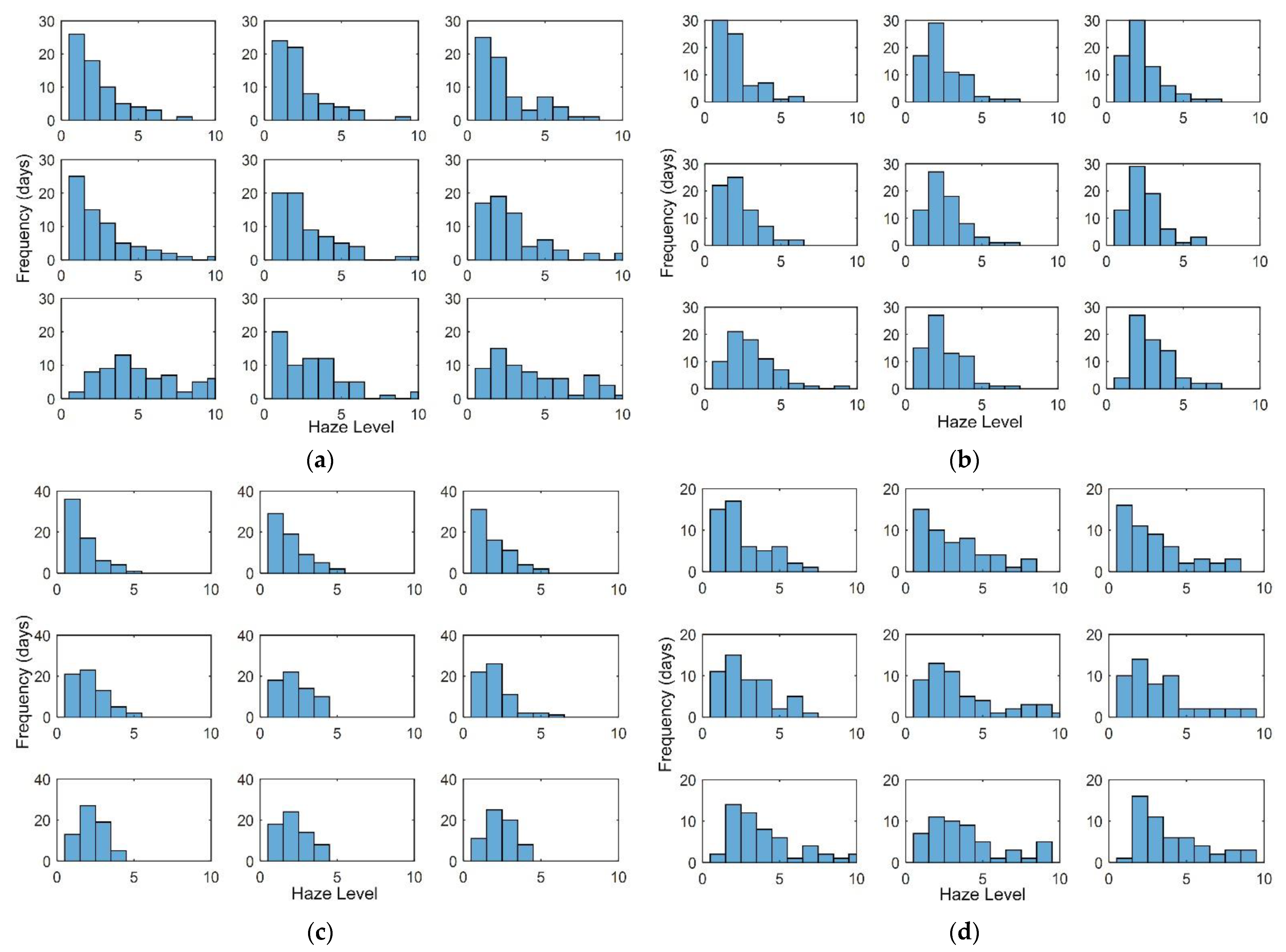
4.1. Analysis of Output Multi-Convolutional Neural Network

We divide the haze prediction results of Beijing in 2014 into nine regions. Further, to visually observe the spatial distribution of haze and the temporal evolution characteristics at the seasonal scale, we divide the results into four seasons and plot the frequency histograms of the haze level. We analyze the overall frequency of haze, some areas with obvious haze characteristics in different seasons and the similarity between different regions. The frequency histograms of haze levels in winter, spring, summer, and autumn are respectively shown in Figure 5a–d.

Then the results are analyzed in three aspects:

(1) Frequency of overall haze; (2) Analysis of the highest and lowest grade areas; (3) Similarity between blocks.

Figure 5a shows that:

• The concentration of haze in winter is generally high, especially in Block 7, Block 8, and Block 9. Block 7 is average in different levels and has the most severe haze pollution.
• There is a high similarity among Block 3, Block 4 and Block 5, and they have the lowest average of haze levels.
• There is a haze with super-high concentration levels in the middle and southern regions, and these areas have more daily pollution such as that from vehicle emission and urban construction due to high population density.

The frequency histograms of haze levels in spring show:

1.

Overall haze levels in spring are low. Block 1 has the lowest haze level, mainly concentrated between level 1and level 2. The concentration in the blocks adjacent to Block 1 is low, and the trend of increasing concentration follows the increasing speed of distance.

2.

The most extensive average haze level among the nine blocks occurs in Block 7, whose haze levels are concentrated at levels 3 and 4. Block 7 also has severe haze and has low similarity to the surrounding area.

3.

Block 1 and Block 4 have high similarities. Likewise, block 2 is similar to Block 3, and there is a high similarity between Block 5 and Block 8 and Block 9.

Figure 5c shows:

1.

Summer is the season with the weakest pollution in a year. In haze distribution, the pollution in the central region is more severe than in the upper region and weaker than in the lower region. The lower region has the most polluted air and the pollution decreases towards the upper region.

2.

All the haze levels in summer are under level 5. The Block with the lowest average concentration is still Block 1. Block 7 and Block 9 have the highest average concentration.

3.

Blocks 4, 7, 8, and 9 exhibit a high correlation, and Blocks 1, 2, and 3 show a high similarity.

Analyzing the frequency histograms in autumn, we can draw the following conclusions:

1.

The concentration of haze in autumn is generally high with decreasing low levels and increasing severe haze pollution.

2.

Blocks 1, 2, and 4 have mainly low levels, while other blocks have higher haze levels, such as level 8 or level 9.

3.

Block 1 and Block 4 have high similarity, Block 2 and Block 3 have high similarity, Block 5 is similar to Block 6, and the three blocks in the south have high similarity.

From the degree of haze pollution at a seasonal scale, Beijing’s pollution intensity is in the order: autumn > winter > spring > summer.

If the generation of data is related to the geographical location, the spatial distribution of the data is also location-dependent, and the correlation is positive to the distance. There are three distribution forms: clustering, random distribution, and rule distribution. Haze is a kind of data related to location. We conducted a spatial autocorrelation analysis of the prediction results to analyze the distribution of haze in different geographies and the correlation between different regions. We used Global Moran’s I and Local Moran’s I to analyze the global and local spatial characteristics of haze, respectively.

4.2. Results of Spatial Autocorrelation Experiment

In this experiment, Moran scatter plot and the LISA plot were used to analyze and study the spatial relationship of haze in different seasons. Then, the total spatial autocorrelation during the period was analyzed. The global Moran’s I result are shown in

Table 4. Global Moran Index Table.

Season	Winter	Spring	Summer	Autumn
global Moran’s I	0.071	0.052	0.375	0.349

:

The Moran’s I of the haze of Beijing in winter, spring, summer, and autumn is 0.071, 0.052, 0.375, and 0.349. It shows that the haze concentration in the four seasons is positively correlated with the geographical area. This relationship is the strongest in summer and autumn, indicating that the spatial correlation in these two seasons is more prominent. Moran’s I in winter and spring is very close to zero, indicating that the haze randomly occurs in nine blocks in these two seasons, while in summer and autumn, the haze has the characteristics of regional accumulation.

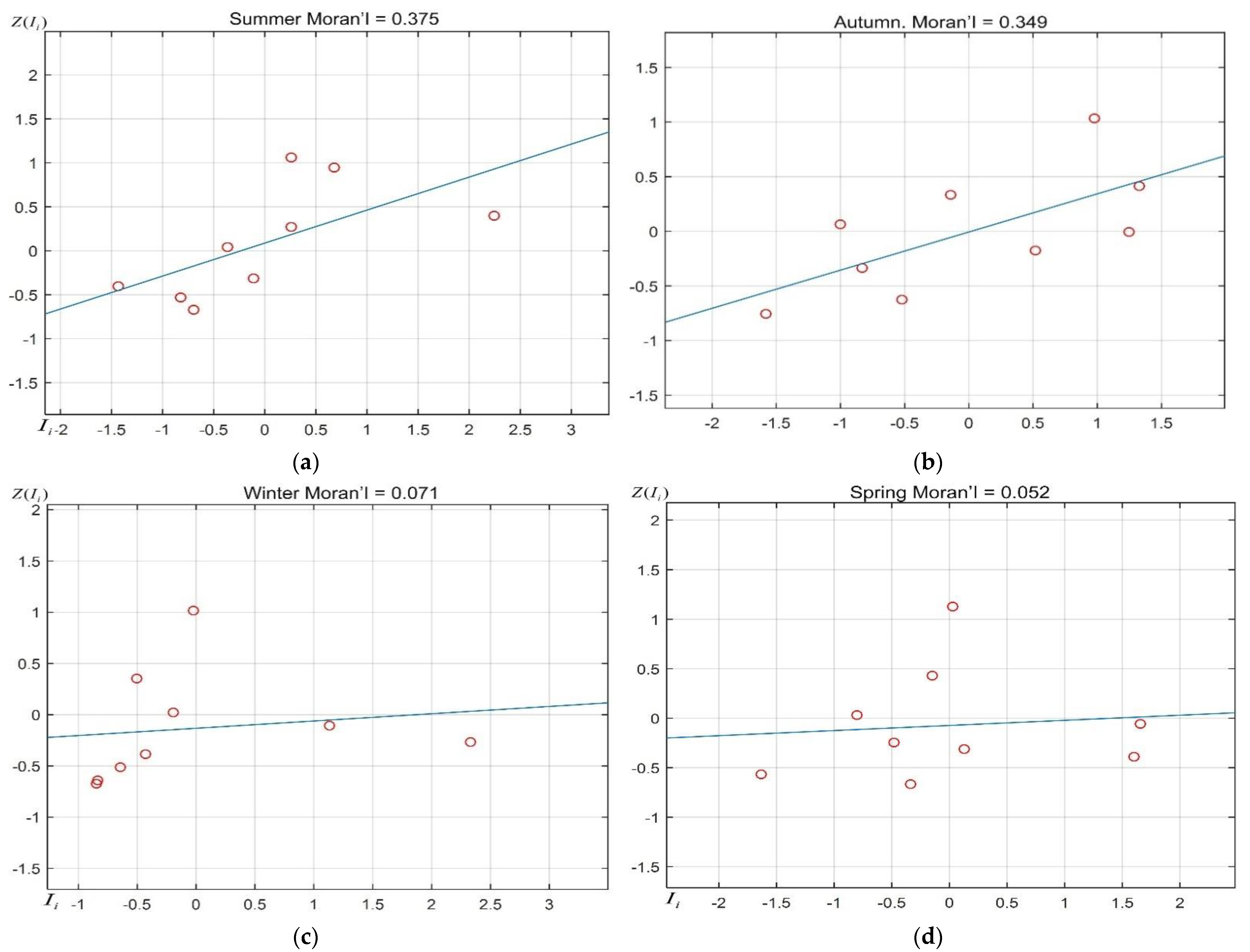
4.2.1. Moran Scatter Plot Results and Analysis

The point in the Moran scatter plot represents an area, and the slope of a linearly fitted curve is equal to the global Moran’s I. According to the global Moran’s I results, there is a high correlation between haze and spatial position in summer and autumn, and the correlation in spring and winter is low. Moran scatter plots for summer, autumn, winter, and spring are shown in Figure 6a–d.

Figure 6a shows that four blocks are in the first quadrant, one block is in the second quadrant, and four blocks are in the third quadrant, and there are generally positive correlation characteristics. Blocks 5, 7, 8, and 9 are in the first quadrant, exhibiting the characteristics of high–high, which means that the haze levels in these four blocks are high, and there is a high positive correlation. Block 4 is in the second quadrant and has a characteristic of low–high. Blocks 1, 2, 3, and 6 are located in the third quadrant, exhibiting a low–low characteristic, and the haze levels of the four blocks are low. In general, the overall characteristics of haze in summer are aggregation type, including high concentration aggregation and low concentration aggregation.

Figure 6b shows two blocks in the first quadrant, two blocks in the second quadrant, three blocks in the third quadrant, and two blocks in the fourth quadrant, which generally show a positive correlation. Blocks 8 and 9 located in the first quadrant exhibit high–high characteristics. Block 4 and Block 6 are in the second quadrant, exhibiting the characteristics of low–high. Blocks 1, 2, and 3 are in the third quadrant, exhibiting low–low characteristics. Finally, Blocks 5 and 7 are in the fourth quadrant exhibiting a ‘high–low’ characteristic. In general, the haze aggregation in autumn is worse than in summer, but there are fewer isolated points, and the overall appearance is aggregated.

The global Moran’s I is small in spring and winter, and the correlation between haze and geographic location is generally weak. There is no block with ‘high–high’ characteristics in the spring, and the other three characteristics are evenly distributed. The coefficient of positive correlation of the overall haze is also low, and the distribution is discrete. There is no high–high characteristic in winter, but there are more low–low blocks, and the correlation is better than in spring. The remaining low-concentration areas surround two high-concentration areas, and the overall distribution shows low concentration aggregation.

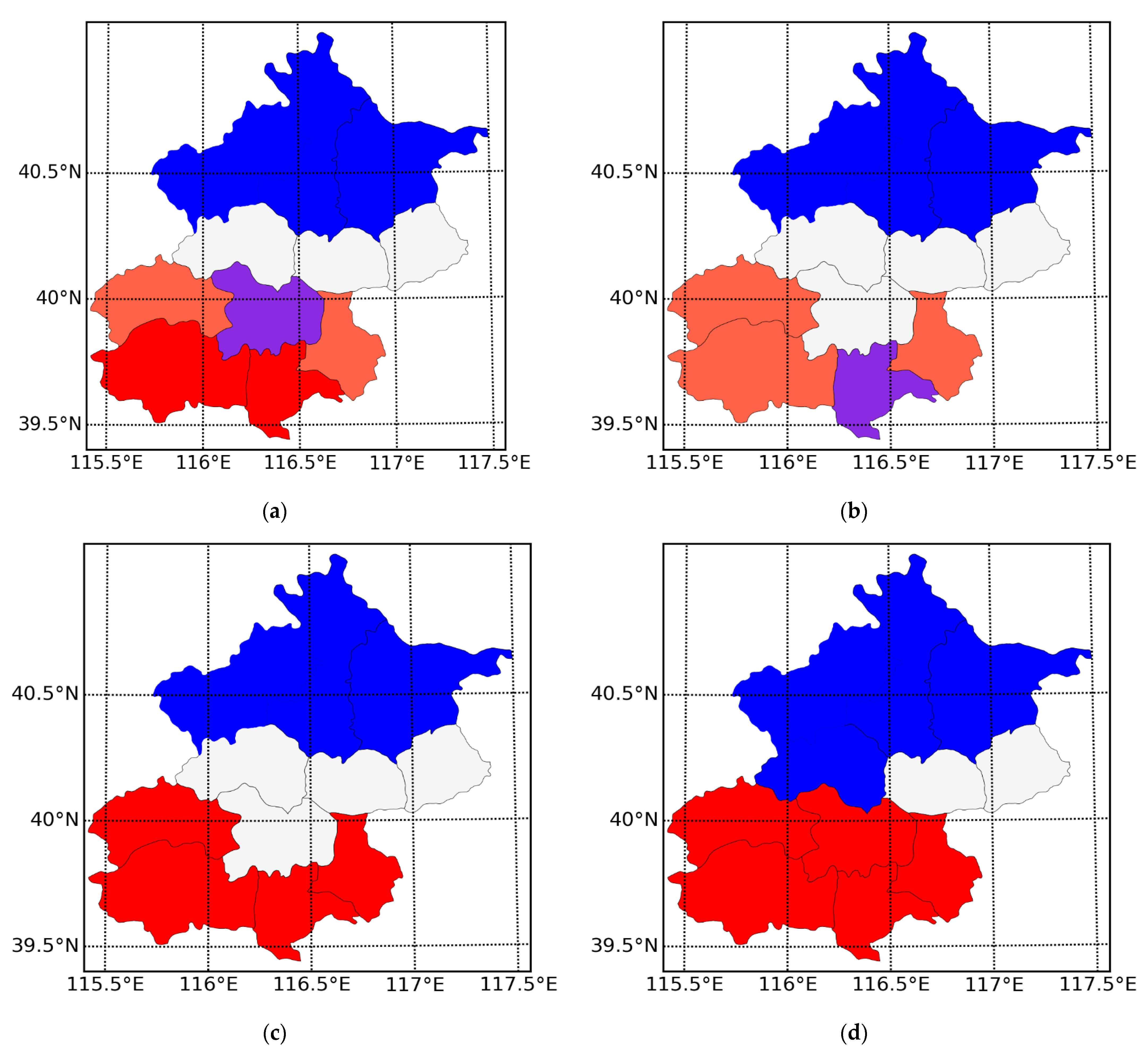
4.2.2. Results and Analysis of LISA Cluster Map

We also use the LISA to visualize the haze aggregation characteristics of the nine blocks. The autoregressive analysis of the local space of nine blocks, combined with the block information table in Table 1, explains the specific spatial location and the saliency of agglomeration. The saliency is the Z value used in the theoretical introduction. In the experiment of this section, the Geoda tool is used for LISA analysis. We use red for H-H, blue for L-L, pink for H-L, and purple for L-H. The LISA maps of winter, spring, summer, and autumn are shown in Figure 7a–d.

From the LISA map of Figure 7a, the low agglomeration area is in northern Beijing in winter, and the high agglomeration area is in the south of Beijing. The low agglomeration area is larger than the high agglomeration area. Thus, the central area of Beijing is the L-H type, where the haze concentration in the winter is far lower than the haze concentration of the surrounding area.

Compared with the winter, the concentration in Block 8 becomes the ‘L-H’ type, and the ‘Fangshan’ in Block 7 becomes the ‘H-L’ type. As a result, the haze pollution in the middle part of the high-concentration area in spring is degraded, so that the ‘H-H’ agglomeration area disappears in the spring, and the ‘L-L’ low-concentration area is the same as the winter consisting of the four areas of the northern area.

As shown in Figure 7c, the agglomeration characteristics in summer are apparent, and the northern blocks are still low-concentration areas. However, the haze concentration in southern Beijing begins to rise, forming an H-H agglomeration area.

Figure 7d shows that the central area of Beijing has become a high-aggregation pattern, which further expands into the south. In contrast, the haze concentration in the north has been in the ‘L-L’ agglomeration type.

The LISA maps for the above four seasons all pass the 5% significance level test, and spatial correlation types of regions in different seasons are shown in

Table 5. Spatial correlation types of regions in different seasons.

Seasons	H-H	H-L	L-L	L-H
Winter	Fangshan, Daxing	Mentougou, Tongzhou	Yanqing, Huairou, Miyun, Changping	Metropolitan Area
Spring	-	Mentougou, Fangshan, Tongzhou	Yanqing, Huairou, Miyun, Changping	Daxing
Summer	Mentougou, Fangshan, Daxing, Tongzhou	-	Yanqing, Huairou, Miyun	-
Autumn	Mentougou, Fangshan, Daxing, Tongzhou, Metropolitan Area	-	Yanqing, Huairou, Miyun, Changping	-

.

The results in Table 5 are arranged in chronological order from top to bottom. Thus, we can analyze the temporal evolution of haze at the seasonal scale.

(1)

The Yanqing, Huairou, and Miyun in the north of Beijing are stable low-concentration areas. As a result, the overall pollution level is low, and the seasonal impact is small. Changping is also relatively stable and only becomes a non-aggregation zone in summer.

(2)

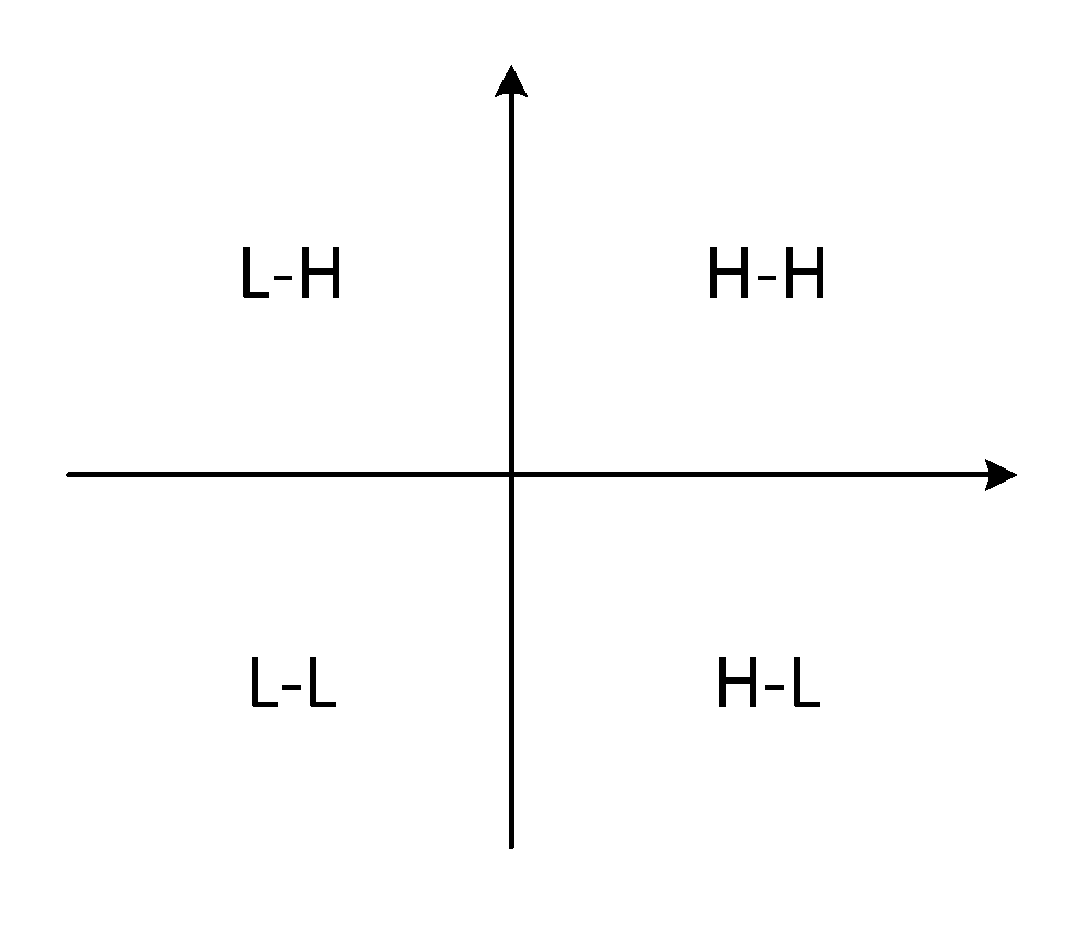
Fangshan in winter is the ‘H-H’ agglomeration area, which became the ‘H-L’ agglomeration area in the spring, indicating the concentration of haze in the vicinity of Fangshan has decreased in the spring.

(3)

Mentougou and Tongzhou have high haze concentrations in summer and autumn, affecting the haze level of the surrounding areas, forming a high concentration area in southern Beijing and the Fangshan and Daxing.

(4)

The areas belonging to ‘H-L’ and ‘L-H’ are easily affected by the haze around them and become high or low accumulation areas in summer and autumn, improving spatial autocorrelation.

5. Discussion

In this paper, we propose a multi-convolution haze-prediction model to predict the daily haze pollution level in different areas of Beijing. We divide the predictions into nine regions and four seasons to study the fine-grained haze pollution and time characteristics. We use the haze level frequency histograms to present the results. From the degree of haze pollution at the seasonal scale, the intensity of haze pollution in Beijing is in the order: autumn > winter > spring > summer. From the distribution of the pollution, the overall pollution in northern Beijing is weak, and the seasonal changes are also small. On the other hand, the haze pollution in the southern regions is intense and shows an aggregation trend.

Moreover, we use the global Moran’s I to measure the correlation between haze and geographical location. The results show that, in general, haze in summer and autumn has regional aggregation characteristics, while in winter and spring the haze distribution is relatively random.

Since the global Moran’s I can only reflect the overall correlation between the haze and the geographical location, we use the local Moran’s I, the Moran scatter plot and the Local Indicators of Spatial Association (LISA) to study the spatial characteristics of haze in the vicinity. The results show that there are obvious agglomeration areas in summer and autumn, while the aggregation effects in spring and winter were relatively weak. Thus, the spatial distribution of haze in Beijing is as follows: the southern region presents a high-high agglomeration, while the northern region exhibits a low-low agglomeration. The temporal evolution of haze on the seasonal scale is according to the chronological order of winter, spring, and summer to autumn, the haze gradually becoming agglomerated.

6. Conclusions

Inspired by the idea of YOLO and other object detection convolutional neural networks, this paper cuts the remote sensing image, analyzes the haze concentration in different areas qualitatively and quantitatively, and derives the spatial laws of different seasons to predict and analyze the haze in a finer time dimension. This paper first proposes the structure of the multi-convolution joint neural network, classifies the spatio-temporal data of haze in the Beijing area by block level, and carries out the frequency statistical analysis method on the output results of the multi-convolution joint neural network. First, the frequency of occurrence of haze levels was displayed and analyzed accordingly. Then, to analyze the results more finely, the Moran’s I of spatial autocorrelation analysis was used in subsequent research to analyze the spatial relationship between each block. Then, to analyze the haze’s temporal and spatial evolution more intuitively, the spatial variation of the haze is analyzed in the LISA cluster map on the time unit of the seasonal scale. Finally, it is concluded that the temporal and spatial distribution of haze in the Beijing area is high in the south and low in the north. Moreover, its temporal and spatial evolution characteristics on a seasonal scale are that, according to the time changes from winter, spring, summer to autumn, the relationship of the haze concentration between each sub-region gradually changes from a discrete state to a concentrated state.

References

1. Zhang, M.; Song, Y.; Cai, X. A health-based assessment of particulate air pollution in urban areas of Beijing in 2000–2004. Sci. Total Environ. 2007, 376, 100–108. [Google Scholar] [CrossRef]
2. Boldo, E.; Medina, S.; Le Tertre, A.; Hurley, F.; Mücke, H.-G.; Ballester, F.; Aguilera, I. Apheis: Health impact assessment of long-term exposure to PM 2.5 in 23 European cities. Eur. J. Epidemiol. 2006, 21, 449–458. [Google Scholar] [CrossRef]
3. Zhang, R.; Jing, J.; Tao, J.; Hsu, S.-C.; Wang, G.; Cao, J.; Lee, C.S.L.; Zhu, L.; Chen, Z.; Zhao, Y. Chemical characterization and source apportionment of PM 2.5 in Beijing: Seasonal perspective. Atmos. Chem. Phys. 2013, 13, 7053–7074. [Google Scholar] [CrossRef] [Green Version]
4. Prospero, J.M.; Olmez, I.; Ames, M. Al and Fe in PM 2.5 and PM 10 suspended particles in south-central Florida: The impact of the long range transport of African mineral dust. Water Air Soil Pollut. 2001, 125, 291–317. [Google Scholar] [CrossRef]
5. Chen, X.; Yin, L.; Fan, Y.; Song, L.; Ji, T.; Liu, Y.; Tian, J.; Zheng, W. Temporal evolution characteristics of PM2.5 concentration based on continuous wavelet transform. Sci. Total Environ. 2020, 699, 134244. [Google Scholar] [CrossRef]
6. Dankwa, S.; Zheng, W.; Gao, B.; Li, X. Terrestrial Water Storage (TWS) Patterns Monitoring in the Amazon Basin Using Grace Observed: Its Trends and Characteristics. In Proceedings of the IGARSS 2018—2018 IEEE International Geoscience and Remote Sensing Symposium, Valencia, Spain, 22–27 July 2018; pp. 768–771. [Google Scholar]
7. Ding, Y.; Tian, X.; Yin, L.; Chen, X.; Liu, S.; Yang, B.; Zheng, W. Multi-scale Relation Network for Few-Shot Learning Based on Meta-learning. In Proceedings of the International Conference on Computer Vision System (2019), Thessaloniki, Greece, 23–25 September 2019; pp. 343–352. [Google Scholar]
8. Zhou, Y.; Zheng, W.; Shen, Z. A New Algorithm for Distributed Control Problem with Shortest-Distance Constraints. Math. Probl. Eng. 2016, 2016, 1604824. [Google Scholar] [CrossRef]
9. Pandolfi, M.; Gonzalez-Castanedo, Y.; Alastuey, A.; Jesus, D.; Mantilla, E.; De La Campa, A.S.; Querol, X.; Pey, J.; Amato, F.; Moreno, T. Source apportionment of PM 10 and PM 2.5 at multiple sites in the strait of Gibraltar by PMF: Impact of shipping emissions. Environ. Sci. Pollut. Res. 2011, 18, 260–269. [Google Scholar] [CrossRef]
10. Li, X.; Zheng, W.; Yin, L.; Yin, Z.; Song, L.; Tian, X. Influence of social-economic activities on air pollutants in Beijing, China. Open Geosci. 2017, 9, 314–321. [Google Scholar] [CrossRef] [Green Version]
11. Liu, S.; Gao, Y.; Zheng, W.; Li, X. Performance of two neural network models in bathymetry. Remote Sens. Lett. 2015, 6, 321–330. [Google Scholar] [CrossRef]
12. Ni, X.; Yin, L.; Chen, X.; Liu, S.; Yang, B.; Zheng, W. Semantic representation for visual reasoning. MATEC Web Conf. 2019, 277, 02006. [Google Scholar] [CrossRef]
13. Tang, Y.; Liu, S.; Deng, Y.; Zhang, Y.; Yin, L.; Zheng, W. Construction of force haptic reappearance system based on Geomagic Touch haptic device. Comput. Methods Programs Biomed. 2020, 190, 105344. [Google Scholar] [CrossRef] [PubMed]
14. Zheng, W.; Li, X.; Xie, J.; Yin, L.; Wang, Y. Impact of human activities on haze in Beijing based on grey relational analysis. Rend. Lincei 2015, 26, 187–192. [Google Scholar] [CrossRef]
15. Zheng, W.; Li, X.; Yin, L.; Wang, Y. The retrieved urban LST in Beijing based on TM, HJ-1B and MODIS. Arab. J. Sci. Eng. 2016, 41, 2325–2332. [Google Scholar] [CrossRef]
16. Yin, L.; Li, X.; Zheng, W.; Yin, Z.; Song, L.; Ge, L.; Zeng, Q. Fractal dimension analysis for seismicity spatial and temporal distribution in the circum-Pacific seismic belt. J. Earth Syst. Sci. 2019, 128, 22. [Google Scholar] [CrossRef] [Green Version]
17. Schwartz, J.; Laden, F.; Zanobetti, A. The concentration-response relation between PM (2.5) and daily deaths. Environ. Health Perspect. 2002, 110, 1025–1029. [Google Scholar] [CrossRef] [Green Version]
18. Franklin, M.; Zeka, A.; Schwartz, J. Association between PM 2.5 and all-cause and specific-cause mortality in 27 US communities. J. Expo. Sci. Environ. Epidemiol. 2007, 17, 279–287. [Google Scholar] [CrossRef] [Green Version]
19. Tucker, W.G. An overview of PM2. 5 sources and control strategies. Fuel Process. Technol. 2000, 65, 379–392. [Google Scholar] [CrossRef]
20. Liu, S.; Wang, L.; Liu, H.; Su, H.; Li, X.; Zheng, W. Deriving bathymetry from optical images with a localized neural network algorithm. IEEE Trans. Geosci. Remote Sens. 2018, 56, 5334–5342. [Google Scholar] [CrossRef]
21. Ma, Z.; Zheng, W.; Chen, X.; Yin, L. Joint embedding VQA model based on dynamic word vector. PeerJ Comput. Sci. 2021, 7, e353. [Google Scholar] [CrossRef] [PubMed]
22. Zheng, W.; Li, X.; Yin, L.; Wang, Y. Spatiotemporal heterogeneity of urban air pollution in China based on spatial analysis. Rend. Lincei 2016, 27, 351–356. [Google Scholar] [CrossRef]
23. Zheng, W.; Liu, X.; Yin, L. Research on image classification method based on improved multi-scale relational network. PeerJ Comput. Sci. 2021, 7, e613. [Google Scholar] [CrossRef]
24. Zheng, W.; Yin, L.; Chen, X.; Ma, Z.; Liu, S.; Yang, B. Knowledge base graph embedding module design for Visual question answering model. Pattern Recognit. 2021, 120, 108153. [Google Scholar] [CrossRef]
25. Zheng, W.; Liu, X.; Ni, X.; Yin, L.; Yang, B. Improving Visual Reasoning Through Semantic Representation. IEEE Access 2021, 9, 91476–91486. [Google Scholar] [CrossRef]
26. Zheng, W.; Liu, X.; Yin, L. Sentence Representation Method Based on Multi-Layer Semantic Network. Appl. Sci. 2021, 11, 1316. [Google Scholar] [CrossRef]
27. Zhao, C.-X.; Wang, Y.-Q.; Wang, Y.-J.; Zhang, H.-L.; Zhao, B.-Q. Temporal and spatial distribution of PM2. 5 and PM10 pollution status and the correlation of particulate matters and meteorological factors during winter and spring in Beijing. Huan Jing Ke Xue Huanjing Kexue 2014, 35, 418–427. [Google Scholar] [PubMed]
28. Ando, M.; Katagiri, K.; Tamura, K.; Yamamoto, S.; Matsumoto, M.; Li, Y.; Cao, S.; Ji, R.; Liang, C. Indoor and outdoor air pollution in Tokyo and Beijing supercities. Atmos. Environ. 1996, 30, 695–702. [Google Scholar] [CrossRef]
29. Gehrig, R.; Buchmann, B. Characterising seasonal variations and spatial distribution of ambient PM10 and PM2. 5 concentrations based on long-term Swiss monitoring data. Atmos. Environ. 2003, 37, 2571–2580. [Google Scholar] [CrossRef]
30. Zhang, Y.-L.; Cao, F. Fine particulate matter (PM 2.5) in China at a city level. Sci. Rep. 2015, 5, 14884. [Google Scholar] [CrossRef] [Green Version]
31. Zhao, X.; Zhang, X.; Xu, X.; Xu, J.; Meng, W.; Pu, W. Seasonal and diurnal variations of ambient PM2.5 concentration in urban and rural environments in Beijing. Atmos. Environ. 2009, 43, 2893–2900. [Google Scholar] [CrossRef]
32. Fuller, G.W.; Carslaw, D.C.; Lodge, H.W. An empirical approach for the prediction of daily mean PM10 concentrations. Atmos. Environ. 2002, 36, 1431–1441. [Google Scholar] [CrossRef]
33. Dong, M.; Yang, D.; Kuang, Y.; He, D.; Erdal, S.; Kenski, D. PM2.5 concentration prediction using hidden semi-Markov model-based times series data mining. Expert Syst. Appl. 2009, 36, 9046–9055. [Google Scholar] [CrossRef]
34. Lee, H.; Liu, Y.; Coull, B.; Schwartz, J.; Koutrakis, P. A novel calibration approach of MODIS AOD data to predict PM2.5 concentrations. Atmos. Chem. Phys. 2011, 11, 7991–8002. [Google Scholar] [CrossRef] [Green Version]
35. Ordieres, J.; Vergara, E.; Capuz, R.; Salazar, R. Neural network prediction model for fine particulate matter (PM2.5) on the US–Mexico border in El Paso (Texas) and Ciudad Juárez (Chihuahua). Environ. Model. Softw. 2005, 20, 547–559. [Google Scholar] [CrossRef]
36. Reid, C.E.; Jerrett, M.; Petersen, M.L.; Pfister, G.G.; Morefield, P.E.; Tager, I.B.; Raffuse, S.M.; Balmes, J.R. Spatiotemporal prediction of fine particulate matter during the 2008 Northern California wildfires using machine learning. Environ. Sci. Technol. 2015, 49, 3887–3896. [Google Scholar] [CrossRef] [PubMed]
37. He, L.; Li, H.; Liu, F.; Liu, N.; Sun, Z.; He, Z. Multi-patch convolution neural network for iris liveness detection. In Proceedings of the 2016 IEEE 8th International Conference on Biometrics Theory, Applications and Systems (BTAS), Niagara Falls, NY, USA, 6–9 September 2016; pp. 1–7. [Google Scholar]
Figure 2. The structure of the multi-convolution neural network.
Atmosphere 12 01408 g002
Figure 3. Spatial adjacency diagram.
Atmosphere 12 01408 g003
Figure 4. Moran scatter image limit relationship.
Atmosphere 12 01408 g004
Figure 5. The frequency histograms of haze levels in (a) winter. (b) spring. (c) summer. (d) autumn.
Atmosphere 12 01408 g005
Figure 6. The Moran scatter plot in and respectively. (a) summer, (b)autumn, (c) winter, and (d) spring.
Atmosphere 12 01408 g006
Figure 7. LISA map of the nine regions in (a) winter. (b) spring. (c) summer. (d) autumn.
Atmosphere 12 01408 g007