Comparison of Seasonal foEs and fbEs Occurrence Rates Derived from Global Digisonde Measurements

Abstract

A global climatology of sporadic-E occurrence rates (ORs) based on ionosonde measurements is presented for the peak blanketing frequency, fbEs, and the ordinary mode peak frequency of the layer, foEs. ORs are calculated for a variety of sporadic-E frequency thresholds: no lower limit, 3, 5, and 7 MHz. Seasonal rates are calculated from 64 Digisonde sites during the period 2006–2020 using ionograms either manually or automatically scaled with ARTIST-5. Both foEs and fbEs ORs peak in the Northern Hemisphere during the boreal summer, with a decrease by roughly a factor of 2–3 in fbEs rates relative to foEs rates without a lower threshold on the sporadic-E intensity. This ratio of foEs to fbEs OR increases with increasing sporadic-E intensity, up to a factor of 5 for the 7 MHz threshold. An asymmetry is observed with the Southern Hemisphere peaks during the austral summer, with slightly lower rates compared with the Northern Hemisphere during the boreal summer. A drastic decrease in ORs is observed for the higher intensity thresholds, such that the fbEs occurrence rates for 7 MHz are nearly zero during most locations and seasons. These updated occurrence rates can be used for future statistical comparisons with GPS radio occultation-based sporadic-E occurrence rates.

1. Introduction

Sporadic-E ($E_s$) is an abnormally strong and thin plasma layer in the E-layer of the ionosphere that can occasional reach peak plasma frequencies greater than the local foF2 [1]. Skywave radio wave propagation can be drastically altered by $E_s$, affecting High Frequency (HF) communications [2,3] and radar operations, including over-the-horizon radar [4]. This potentially significant impact on HF operations motivates the need for an up-to-date global occurrence rate (OR) climatology for varying levels of sporadic-E intensity.

Ref. [5] provides a global climatology of $E_s$ occurrence rates based on ionograms from 45 ionosonde sites. Ionosondes provide a robust method for measuring stronger sporadic-E layers where the peak plasma frequency is above the background ionospheric density [6,7]. While the [5] climatology remains widely used as a standard for global $E_s$ occurrence rates, recent improvements in ionosonde technology [8] and automatic ionogram scaling [9] provide an opportunity to update occurrence rates and distinguish between blanketing and non-blanketing layers [10].

There are many sporadic-E classifications [11] and two commonly used $E_s$ frequency parameters measured by ionosondes: the peak blanketing frequency, fbEs, and the ordinary mode peak frequency of the layer, foEs. Physically, the blanketing frequency corresponds to the peak continuous layer across the entire sporadic-E structure that completely reflects any signal with a frequency below the fbEs [10,12]. The foEs corresponds to the peak frequency reflected by the $E_s$ layer, related to the peak plasma density, which is likely patchy or only present in a limited region of the layer. The difference between these two parameters is important, and both values should be included when creating a global climatology of sporadic-E occurrence rates.

Two thorough reviews on sporadic-E research are provided in Refs. [2,13]. Recently, various studies have used ionosonde data to characterize $E_s$ during or after specific events (i.e., solar eclipse [14], tsunami [15], geomagnetic storms [16,17], etc.). Additionally, regional $E_s$ occurrence rates have been analyzed in Europe [18], South Korea [19], the United States of America [20], China [21], New Zealand [22], and various locations around the globe [23]. Updated sporadic-E maps for foEs $\ge 7$ MHz are outlined in Ref. [24]; however, an updated global map of $E_s$ occurrence rates for varying plasma intensities derived from modern ionosonde data, to our knowledge, has not been produced.

In addition to ionosondes, sporadic-E can be measured from other instruments, such as incoherent scatter radars (ISRs) [25], ground-based global navigation satellite system (GNSS) measurements [26,27,28], and GPS radio occultation (RO) [29,30]. ISR measurements provide the most detailed observations of $E_s$ characteristics and structure [13,31,32], but the limited number of sites across the globe and measurement cadence are lacking for global climatological studies. Ground-based GNSS measurements allow for unprecedented large-scale studies of $E_s$ morphology for strong layers (foEs > 14 MHz) over areas with GNSS networks, such as Japan [26] and China [27,28]. These ground-based measurements provide detailed information on the elongation, orientation, scale-size, and horizontal motion of the layers in addition to regional occurrence rates for exceptionally strong $E_s$ layers.

GPS radio occultation (RO) measurements provide a dense set of global measurements and have recently been used to estimate global $E_s$ occurrence rates [29,30,33,34]. However, the direct relationship between GPS-RO measurements to sporadic-E parameters and intensity are difficult to determine because of the unknown length, orientation, and vertical thickness of the sporadic-E layers [35].

The $E_s$ perturbation to GPS signals relies on the phase delay of the layer with respect to the background, which is proportional to the product of the distance and the index of refraction. The lack of information on the length, orientation, and vertical thickness of the layers generates an uncertainty in the interpretation of GPS-RO measurements [36].

From this, $E_s$ occurrence rates derived from GPS-RO can vary by a factor of five between studies [37,38]. Improving global climatological $E_s$ maps produced by GPS-RO measurements can be accomplished by comparing the RO-based occurrence rates to more direct measurements from ionosondes to map each technique to a specific sporadic-E parameter of interest (e.g., fbEs $\ge 3$ MHz). However, this first requires an updated global set of occurrence rates based on ionosonde measurements, which motivated the current study.

Here, we utilized all available data from the Global Ionospheric Radio Observatory (GIRO) network of Digisondes [39] to produce updated sporadic-E occurrence rates for foEs and fbEs over each available site. Occurrence rates were calculated for a variety of sporadic-E plasma intensities: no lower threshold, 3, 5, and 7 MHz. The direct $E_s$ measurements from ionosondes were used to calculate an updated “ground-truth” for occurrence rates, which can then be used to validate GPS-RO-based occurrence rates in future studies.

2. Methods

2.1. Data Set Development

Ionogram derived sporadic-E parameters automatically scaled using the ARTIST software for Digisondes [9] were downloaded from the GIRO web portal (http://giro.uml.edu/didbase/scaled.php (accessed on 21 November 2021). Additionally, information from the Digital Ionogram Database (https://ulcar.uml.edu/DIDBase/ (accessed on 21 November)) was combined with the scaled parameters to determine the ARTIST software version used for the scaling and ionogram inversion.

Large differences in the fbEs and foEs occurrence rates were found between ARTIST-4 and ARTIST-5 (see Section 2.3), with unrealistically low fbEs values and abnormally high foEs values from ARTIST-4. From this, we limited the Digisonde data to only ionograms either manually scaled or automatically scaled using ARTIST-5. There are sites without a specified auto-scaled software on DIDBase, and, in most cases, the site used a country- or site-specific auto-scaled software. To obtain consistent results these sites were removed from the final data set.

In certain cases, there are times when there are only 10’s to 100’s of ionograms for a specified season for a particular site. Although this is useful to study specific events, these spurious cases can skew the average occurrence rate to higher or lower percentages due to the lack of total data available. To overcome this, when determining an occurrence rate, we required the total number of ionograms to be $>4320$ for seasonal averages. This ensures that the ionogram was operating approximately half of the time period assuming an ionogram was collected every 15 min (the regular measurement cadence for most Digisondes).

The ionograms and scaling of certain sites with abnormal results in relation to nearby sites were analyzed to determine the reliability of $E_s$ estimates. From this, two sites were removed from the analysis (URSI station codes WU430 and BP440) as a result of foEs OR estimates below two standard deviations from the spatial mean calculated from nearby sites. These exceptionally low ORs are not present in previous East Asia sector climatologies for either ionosonde [5] or GPS-RO [30,37,38]-based measurements.

In fact, Refs. [5,30] showed elevated occurrence rates and activity in this East Asia sector, which supports the removal of these two sites from the climatological calculations. URSI station code RO041 was also removed due to a lack of fbEs measurements during this time period resulting in fbEs ORs of zero. All other sites were used for the analysis as long as the conditions on the number of ionograms during a given time period were satisfied.

To calculate the occurrence rates, both the number of sporadic-E measurements over a time period and the total number of measurements is required. One method for calculating the total number of vertical ionograms during a given period is to use the number of foF2 measurements as a proxy. However, in our analysis, it was clear that this can easily lead to instances where the $E_s$ occurrence rate is greater than 100%.

One specific case is shown in Figure 1 where a strong blanketing $E_s$ layer completely shielded the F2 peak and foF2 could not be determined. Since we are unable to physically check every ionogram, we alternatively used the confidence score (CS) reported by ARTIST-5 as an indicator of the total number of ionograms in a given time period. For example, the occurrence rate for fbEs ≥ 3 MHz is calculated by

$$OR(fbEs\ge 3\mathrm{MHz})=\frac{N(fbEs\ge 3\mathrm{MHz})}{N_{CS}},$$

(1)

where $OR(fbEs\ge 3\mathrm{MHz})$ is the occurrence rate for fbEs greater than or equal to 3 MHz, $N(fbEs\ge 3\mathrm{MHz})$ is the number of fbEs measurements during the time period of interest above the 3 MHz threshold, and $N_{CS}$ is the total number of vertical ionograms provided by the number of confidence scores. In addition to the 3 MHz threshold, 5 and 7 MHz thresholds were also analyzed along with a general sporadic-E occurrence rate with no lower boundary (any foEs or fbEs measurement), and this same technique was used for the foEs occurrence rates.

The 3, 5, and 7 MHz thresholds follow the methodology and results provided in Ref. [5]. It must be noted that most ionosondes run into frequency allocation and sensitivity issues below ∼1.5 MHz, and thus there is a natural lower threshold for ionosonde-based $E_s$ measurements that is not present with Incoherent Scatter Radar (ISR) measurements (see [40]).

The final dataset resulted in a total of 64 stations with data from 2006 through 2020 (Figure 2). The data was split into seasons of boreal winter (December, January, and February), spring (March, April, and May), summer (June, July, and August), and fall (September, October, and November), and by the ARTIST-5 reported strength of $E_s$. All averages were performed for the entire day with no separation between local times (i.e., night and day), as the primary goal of this effort is to provide a baseline for statistical comparison against GPS-RO-derived occurrence rates.

The background E-layer density was not removed using the techniques outlined in Ref. [41] to calculate the strength of the metallic ion layer. The occurrence rates were averaged for each year, and the final values displayed are the averages over the range of years. A simple estimate of uncertainty is provided by the standard deviation over the range of years. Some stations only have data for one year, and thus no standard deviation is reported. It must be noted that there are certainly errors in the automatic ionogram scaling [42]. However, these errors are difficult to quantify as they depend on the site, frequency allocations in the E-region frequency ranges, and other factors that may cause a “false-positive” for sporadic-E.

2.2. Overview of Data from DIDBase and GIRO

As of 26 September 2020, there were a total of 36,113,430 scaled ionograms in the GIRO database from 1988–2020 recorded at 120 sites across the globe, with 31,560,182 ionograms stored in the DIDBase (Figure 3). The majority (81.6%) of ionograms were processed using a version of the software ARTIST, with the remaining scaled from unknown sources (14.4%), the software Autoscala (3.6%), and ParuaAuto (0.2%) from specific persons (0.1%). Notably, the 14.4% scaled from unknown sources were from 15 sites that used either a Dynasonde or IPS-5A for data collection. The other 0.2% were from various days and sites where no scaler or software was reported on DIDBase.

A further breakdown of the ARTIST-scaled data shows that less than 2.5% of ARTIST scaled ionograms are from version 1–3, ∼30% are scaled with ARTIST-4, 15.8% with ARTIST-4.5 and the majority (52.7%) with ARTIST-5. This is notable since only ARTIST-5 has a built-in function to accurately detect blanketing Es, whereas all earlier versions appear to be more focused on the foEs parameter. There are sub-versions of ARTIST as well denoted with a six-digit number. For example, there are two versions of ARTIST-5 with software numbers 500100, and 500200. To simplify the analysis, these sub-versions were ignored and only the overall software version was taken into consideration.

Finally, more ionosondes have been installed over the years, naturally increasing the amount of data available. For example, the number of total ionograms has increased since 1988 by ∼360% following a general second order polynomial trend upwards to approximately four million ionograms in 2019 (Figure 3). To overcome any bias in data analysis due to a lack of data in earlier years, we used strict criteria for the number of ionograms at one site during a given time period (see Section 2.1).

2.3. Comparing ARTIST-4, ARTIST-4.5 and ARTIST-5

The most abundant source of auto-scaled ionosonde data comes from ARTIST-5; however, using only ARTIST-5 data restricts our analysis to years more recent than 2006, and excludes sites that continued to use ARTIST-4, and ARTIST-4.5. For this reason, we compared results from these three versions to highlight differences in auto-scaling. Using SAOExplorer v3.5.3 ionograms were downloaded and reprocessed using the built-in version of ARTIST-5. Due to the time required for reprocessing, only a subset of data in the year 2006 from four sites was analyzed.

As displayed in Figure 4A, four sites were selected to represent the temperate zone in the Northern (EG931) and Southern (LM42B) Hemisphere, the Equatorial Zone (KJ609), and the Auroral Zone (GA762). Subsequently, data from March, June, September, and December of 2006 were reprocessed with ARTIST-5, where data from EG931, LM42B, were initially processed with ARTIST-4, and GA762 with ARTIST-4.5. Most (81.5%) of the data at KJ609 were analyzed with ARTIST-4.5; however, some were analyzed with ARTIST-5.

Figure 4B shows that the foEs differences between ARTIST-4 and ARTIST-5 are most often centered around zero. However, there are many foEs differences above 5 MHz, which is a significant difference for typical sporadic-E layer strengths. This difference is important when using ionosonde measurements as the ground-truth for sporadic-E strengths and motivates the choice to use ARTIST-5 for the occurrence rate calculations.

The trends displayed in Figure 4C show the large differences in occurrence rates calculated using the different versions of ARTIST. While ARTIST-4 (before ∼2006) appears to overestimate foEs occurrence rates, fbEs is rarely measured, which produces occurrence rates near zero. For example, the EG931 fbEs occurrence rates were nearly zero for the ARTIST-4 measurements and increased to above 5% after 2006 when the ARTIST software was upgraded to version 5.

Following these results, the remainder of our analysis was focused solely on ionograms manually scaled or automatically scaled by ARTIST-5. It must be noted that, while sporadic-E estimates from ARTIST-5 are greatly improved over previous versions, any automated process is subject to errors. A long-term comparison of manually scaled and automatically scaled sporadic-E parameters is required to provide a robust estimate of occurrence rate uncertainties by ARTIST-5; however, this uncertainty estimate will not be included in the current analysis.

3. Results and Discussion

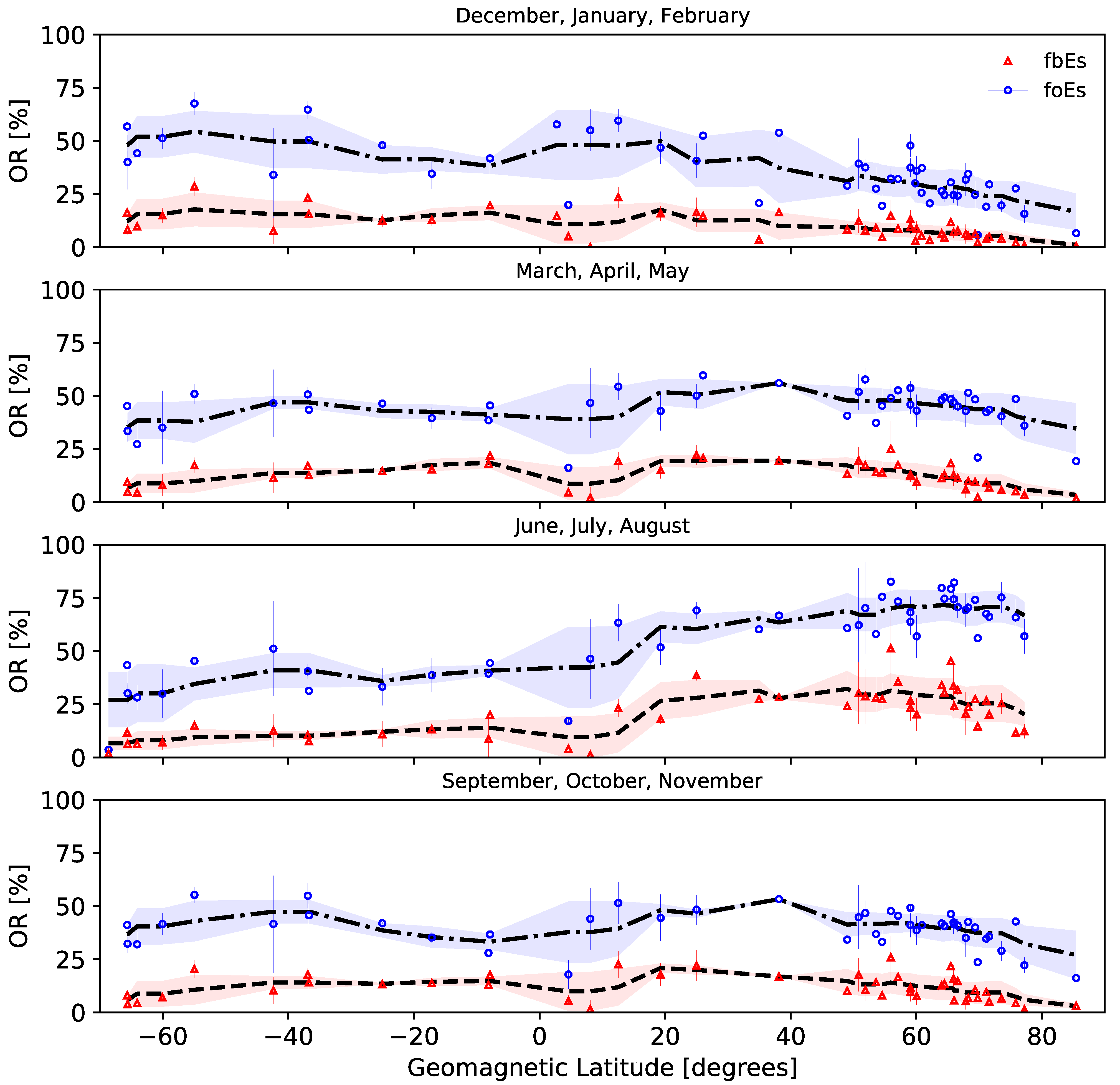
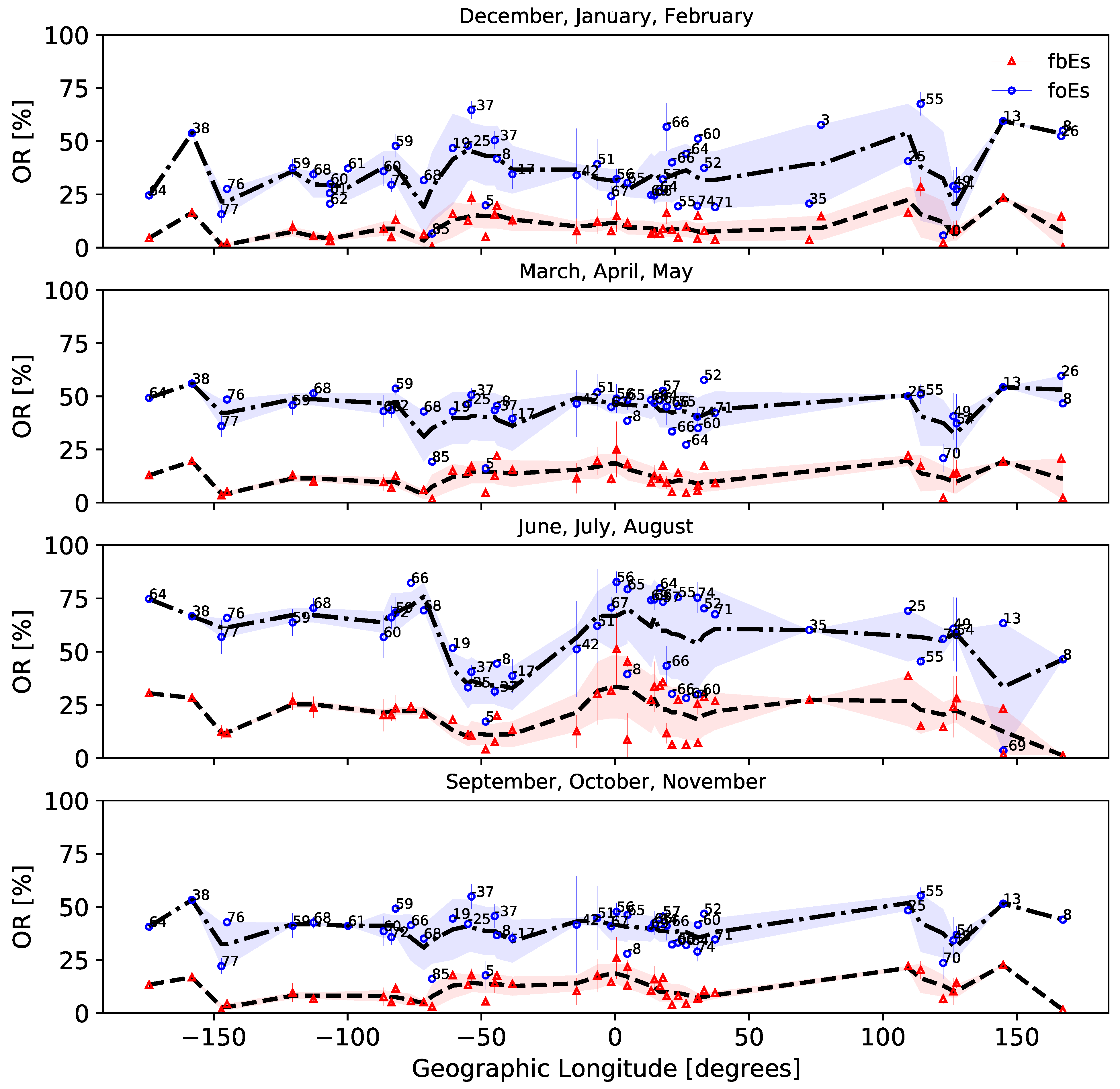
3.1. Total Occurrence Rates: No Lower Threshold

Utilizing data that was auto-scaled using ARTIST-5, we first plotted the available sites on a global map (Figure 2). There were a total of 64 sites that spanned −45° to 80° geographic latitude spanning from 2006 to 2020, which satisfied the criteria outlined in Section 2.1. However, the number of sites and ionograms availability from each year varied widely, from 45 sites in 2006 with an average of 2260 ionograms per month per Digisonde, to 75 sites in 2019 with an average 4260 ionograms per month per ionosonde. To increase the confidence in the occurrence rates for a given season, a lower threshold of 4320 ionograms per site per season was required to use a site in this analysis.

The seasonal occurrence rates calculated for foEs and fbEs without a lower limit on intensity are displayed in Figure 5. The results are displayed as a function of the geomagnetic latitude, as the magnetic dip angle plays a vital role in the wind shear theory for sporadic-E formation (see Ref. [2]). In additional to the uncertainty calculated from the standard deviation over the range of years (error bars), a spatial running average and standard deviation with a $\pm {10}^{\circ }$ window is also displayed. Care must be taken with the spatial trends, as missing data points could be markedly different from the running average. For example, Refs. [37,38] show relatively large changes over short distances with patches of elevated or depleted ORs. The spatial trends as a function of geomagnetic latitude outlined in Figure 5 average out the small scale variation that is observed in the individual sites.

The general trend of maximum occurrence rates in the geomagnetic mid-latitudes is present with peak ORs around 30% for fbEs and 70% for foEs during the boreal summer. Through the wind shear theory, metallic ions produced by meteoroid ablation converge through diurnal and semidiurnal tidal wind shears [2,13]. Ion convergence through the Lorentz force is dependent on the magnetic dip angle, which is maximized at the geomagnetic equator and minimized at the geomagnetic poles for a zonal wind shear. However, formation rates are reduced at the geomagnetic equator because electrons are highly magnetized at E-region altitudes [1], which constrains the electrons to horizontal motion from a zonal wind shear at the equator.

This limits the vertical ion flow through charge separation and subsequent electric fields created by the constrained electrons (see the discussion in Ref. [37]). Through this, a peak in sporadic-E formation is expected at mid-latitudes with reduced rates at the geomagnetic equator and poles. Additionally, meteoric deposits show seasonal variability with maxima during local summer [23,43]. This general behavior is present in Figure 5, with mid-latitude peaks during the local summer. A slight decrease in the rates near the arctic and equatorial zones is also visible as expected through the wind shear theory.

As observed in previous climatologies, an asymmetry between the Northern and Southern Hemispheres is present [5,37,38]. While the austral summer also shows increased ORs in the Southern Hemisphere, the peak magnitudes are less than the Northern peaks during the boreal summer, with rates of 50% and 20% for foEs and fbEs, respectively. The South Atlantic Anomaly (SAA) plays a large role in this asymmetry due to the weaker magnetic field, which reduces the Lorentz force magnitudes required for ion convergence. Fall and Spring OR trends were nearly flat across the range of geomagnetic latitudes, with foEs rates around 40% and fbEs rates around 15%.

Overall, the foEs ORs were larger than the fbEs rates by a factor of 2–3. This difference is due to the stricter criteria placed on fbEs, which must be a continuous metallic ion layer above the ionosonde site that completely blankets radio wave transmissions with frequencies below the fbEs. The foEs corresponds to patchy layers or partially blocked ionosonde sites, which increases the overall likelihood of measurement.

While the general behavior of $E_s$ ORs as a function of geomagnetic latitude are believed to be caused primarily by zonal wind shears, the factors controlling the longitudinal trends are less understood. The relatively small number of global ionosonde sites creates difficulties in developing global maps; however, latitudinal and longitudinal trends can be analyzed. Ultimately, global OR maps require the use of additional datasets, such as GPS-RO, to fill the missing gaps in regions between ionosonde stations.

The ionosonde-derived trends as a function of the geographic longitude are displayed in Figure 6. Large-scale fluctuations are primarily due to changes in geomagnetic latitude. However, OR differences of over 10% can be observed for sites with similar geomagnetic latitudes but varying longitudes. For example, ORs for Santa Maria and Cachoeira Paulista, Brazil (URSI codes SMK29 and CAJ2M) show a nearly 15% difference in ORs during austral summer even though the geomagnetic latitudes are nearly equal at −37${}^{\circ }$. A longitude separation of $9^{\circ }$ indicates that other conditions, such as variations in tidal wind shears or atmospheric gravity waves (AGWs), can affect the measured ORs.

Kelvin–Helmholtz instabilities [44] can modulate $E_s$ layers to form billowy, small-scale structures [26,27,45] that affect both the spatial profiles and ionosonde measurements of the layers. This supports previous global [5,37,38] and regional [28] occurrence rate studies with large variations over relatively short distances. A simple trend as a function of geographic longitude is difficult to extract because of the strong dependence on geomagnetic latitude; however, the variation between regions with similar latitudes indicates a complex formation dependence on additional factors not included in the simple wind shear theory.

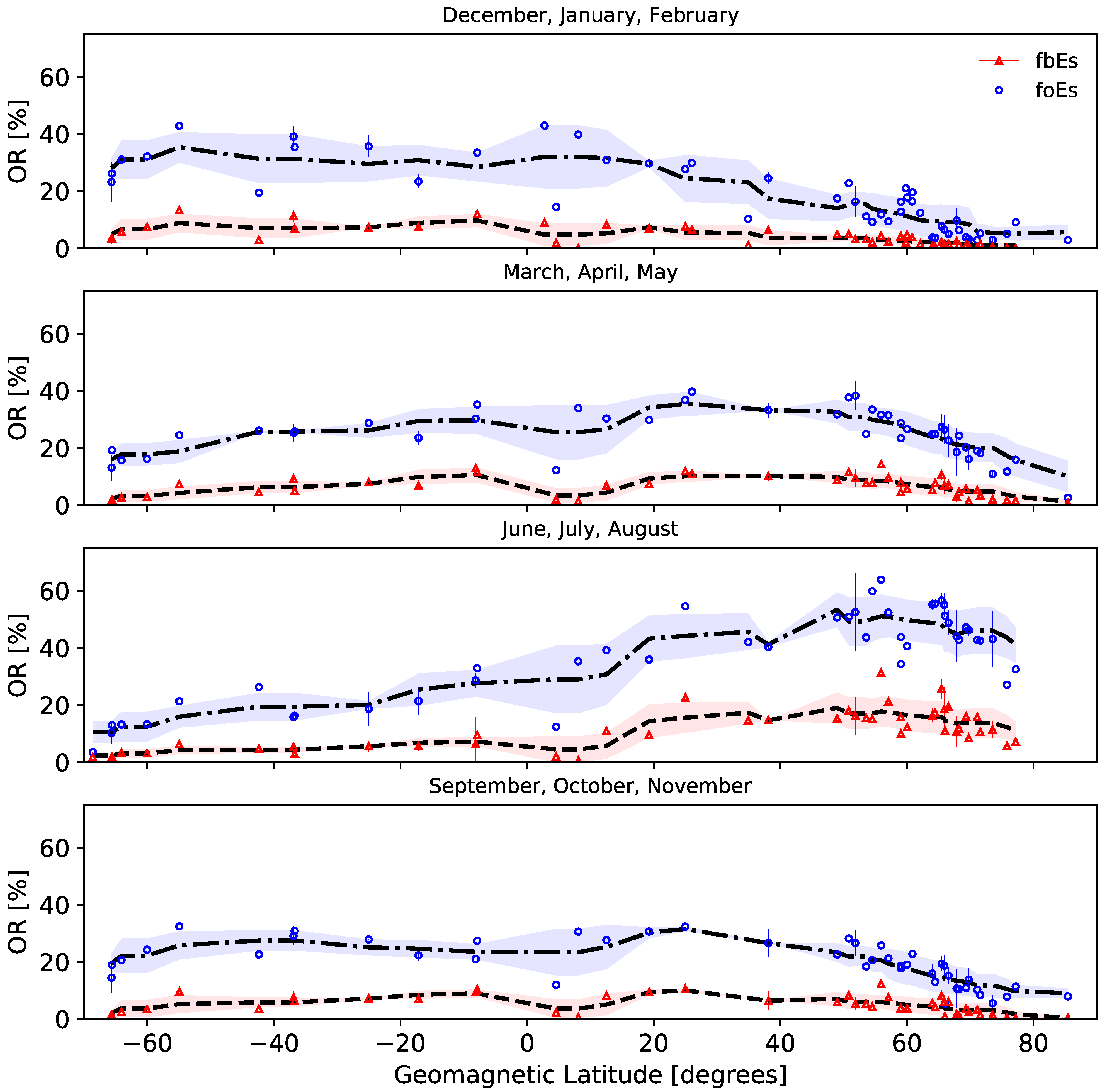
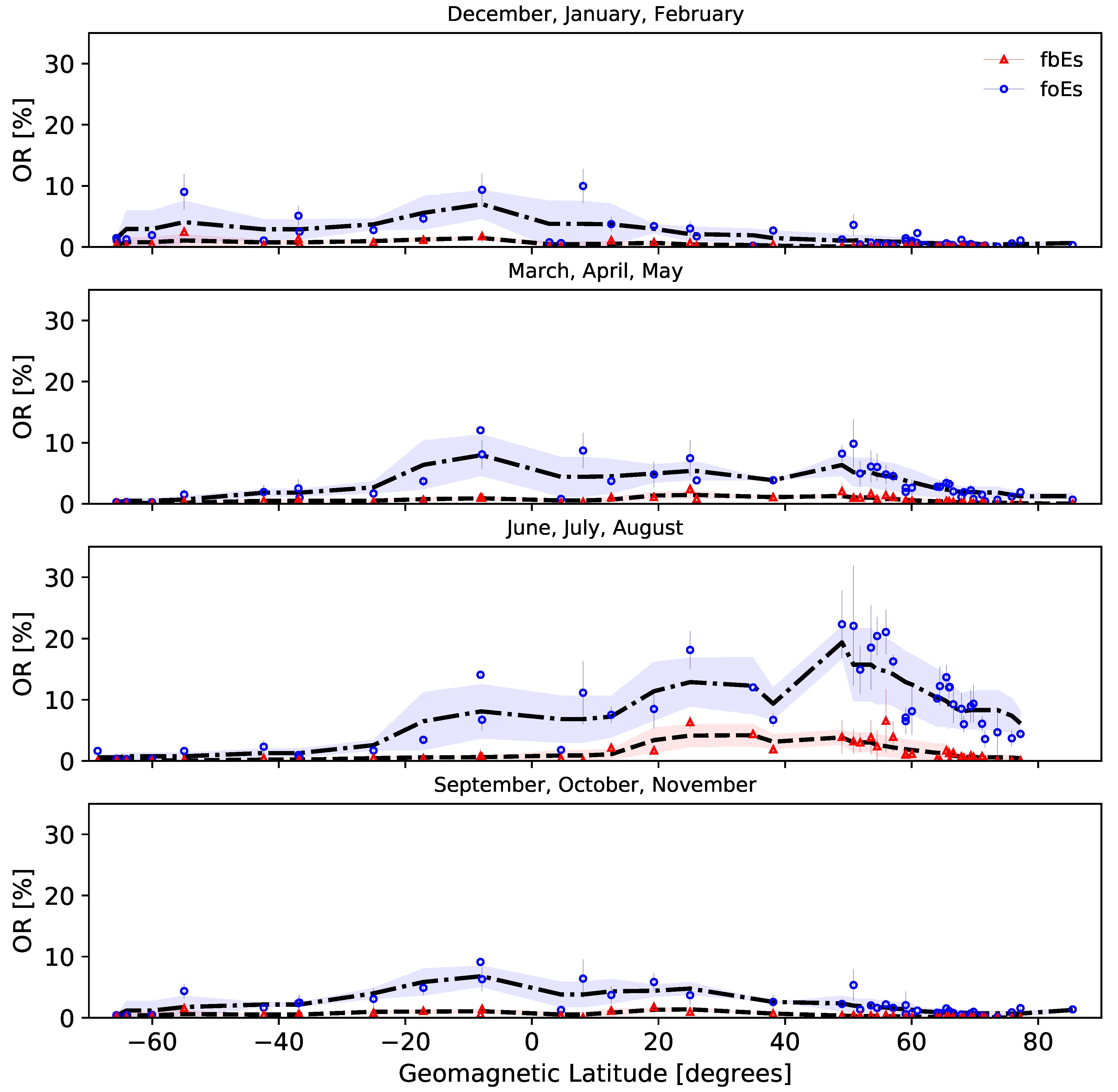
3.2. Three, Five, and Seven MHz Thresholds

ORs for the 3 MHz threshold follow the same general trends as the ORs without a lower limit on intensity, but the magnitudes are reduced by a factor of roughly 2/3 (Figure 7). The peak boreal summer foEs rates are approximately 50% in the Northern Hemisphere, and a peak of 35% is observed in the Southern Hemisphere for the austral summer. Similarly, peak fbEs rates of 15% are observed in the Northern Hemisphere for boreal summer and 10% for the Southern Hemisphere austral summer. Fall and spring foEs peaks are around 30% with fbEs rates ∼10%. In this case, the factor between the foEs and fbEs ORs is slightly larger than 3, which is close to the factor of 2–3 for the rates without a lower threshold.

For the 5 MHz threshold (Figure 8), similar trends are observed with peak foEs ORs below 20% and fbEs rates peaking around 5% in the Northern Hemisphere during the boreal summer. Interestingly, a peak foEs in the Southern Hemisphere of approximately 10% occurs around −10${}^{\circ }$ geomagnetic latitude during the austral summer, fall, and spring. The fbEs rates are very low (below 1%) for the majority of locations and seasons, with a noticeable increase in the Northern Hemisphere during the boreal summer. For this threshold, the foEs to fbEs ratio is around 4 for most latitudes and seasons.

Finally, the 7 MHz threshold ORs (Figure 9) show trends similar to the 5 MHz threshold, but with peak values nearly a factor of 4 lower. Peak foEs rates of ∼5% occur in the Northern Hemisphere during the boreal summer, with fbEs rates less than 1%. For the other seasons, the fbEs rates are essentially zero, while the foEs rates have a peak of approximately 2% near −10${}^{\circ }$ geomagnetic latitude. Here, the foEs to fbEs ratio of rates is around 5, which is larger than the ratios for the other lower thresholds.

In comparison with previous climatologies, the general trends as a function of geomagnetic latitude match the recent GPS-RO-derived trends outlined in Refs. [37,38]. The occurrence rate magnitudes in Ref. [37], which peak near 10% during local summer in the mid-latitudes align well with our fbEs $\ge 3$ MHz magnitudes (Figure 7). Conversely, the mid-latitude local summer OR magnitudes of ∼50% found in Ref. [38] are in agreement with our foEs $\ge 3$ MHz rates. This provides insight into the OR differences between GPS-RO studies and should be explored in more detail. The OR peaks of 25% for fEs $\ge 5$ MHz found in Ref. [5] are slightly larger than the peak foEs magnitudes of ∼20% displayed in Figure 8 for the same threshold.

Additionally, the peak occurs near the geomagnetic equator in the East Asia sector in Ref. [5] while the current results show a mid-latitude peak with reduced rates near the equator. These differences can most likely be attributed to updates in ionosonde equipment and processing tools. It must also be noted that the fEs measurements in Ref. [5] likely correspond to fxEs rather than foEs, and thus a slight difference in OR magnitudes should be expected.

4. Conclusions

Seasonal foEs and fbEs occurrence rates were calculated globally for a variety of $E_s$ intensity thresholds: no lower limit, 3, 5, and 7 MHz. Digisonde data over the period 2006–2020 processed with ARTIST-5 from 64 sites was used to obtain the mean occurrence rates and uncertainties. Large differences in sporadic-E measurements were observed using different versions of automatic scaling software (ARTIST), and the final data was limited to ionograms either processed manually or automatically with ARTIST-5.

From this, the peak $E_s$ formation was found to occur in the Northern Hemisphere during the boreal summer (June, July, and August), matching the results of many previous studies. The occurrence rates heavily depended on the intensity thresholds, with higher intensities occurring less often. The fbEs rates were lower than the foEs rates by a factor of 2–3 without a lower intensity threshold; however, this ratio increased as the intensity threshold increased. This difference is due to the stricter criteria placed on the blanketing layers, which must possess a continuous layer over the ionosonde while the foEs can be patchy or partially cover the site.

The local summer rates in the Northern Hemisphere peak around 70% for foEs, while the fbEs peaks around 30% for no lower limit on the sporadic-E intensity. An asymmetry was observed in the Southern Hemisphere during the austral summer with peak foEs rates around 50% and fbEs rates around 20%. It must be noted that the concentration of Digisonde sites is much larger in the Northern Hemisphere, which poses a problem with proper sampling of the Southern Hemisphere. However, this asymmetry has also been observed in other climatological studies of sporadic-E occurrence. The fall and spring rates were mostly flat with local minima towards the geomagnetic poles and equator.

Occurrence rates for the 3, 5, and 7 MHz thresholds showed similar trends as the rates without a lower limit on intensity, but the peak magnitudes decreased as the threshold increased. The respective peak rates in the Northern Hemisphere during the boreal summer for foEs (fbEs) with 3, 5, and 7 MHz thresholds were approximately: 50% (15%), 20% (5%), and 5% (1%). The Southern Hemisphere peaks showed the same asymmetry as the rates with no lower limit on intensity.

These updated occurrence rates provide a baseline for an updated sporadic-E climatology that can be used as the “ground-truth” for occurrence rate studies with GPS radio occultation, providing a method of attributing a sporadic-E intensity to the many GPS-RO techniques outlined in the literature. The large differences in occurrence rates for the varying intensity thresholds may provide insight into the factor of ∼5 difference in sporadic-E occurrence rates between GPS-RO-based sporadic-E climatology studies: the different techniques likely correspond to different sporadic-E intensities, and future work is required to properly match the different techniques to the results of this analysis.

References

1. Rishbeth, H.; Garriott, O.K. Introduction to Ionospheric Physics; Academic Press: Cambridge, MA, USA, 1969. [Google Scholar]
2. Whitehead, J. Recent work on mid-latitude and equatorial sporadic-E. J. Atmos. Terr. Phys. 1989, 51, 401–424. [Google Scholar] [CrossRef]
3. Rice, D.; Sojka, J.; Eccles, J.; Raitt, J.; Brady, J.; Hunsucker, R. First results of mapping sporadic E with a passive observing network. Space Weather 2011, 9, 12001. [Google Scholar] [CrossRef]
4. Fabrizio, G.A. High Frequency over-the-Horizon Radar: Fundamental Principles, Signal Processing, and Practical Applications; McGraw-Hill Education: New York, NY, USA, 2013. [Google Scholar]
5. Smith, E.K. Worldwide Occurrence of Sporadic E; US Department of Commerce; National Bureau of Standards: Gaithersburg, MD, USA, 1957; Volume 582. [Google Scholar]
6. Matsushita, S.; Reddy, C. A study of blanketing sporadic E at middle latitudes. J. Geophys. Res. 1967, 72, 2903–2916. [Google Scholar] [CrossRef]
7. Whitehead, J. The structure of sporadic E from a radio experiment. Radio Sci. 1972, 7, 355–358. [Google Scholar] [CrossRef]
8. Reinisch, B. IONOSONDES and the measurements they make. In Proceedings of the International Reference Ionosphere 2019 Workshop, Nicosia, Cyprus, 2–13 September 2019. [Google Scholar]
9. Galkin, I.A.; Reinisch, B.W. The new ARTIST 5 for all digisondes. Ionosonde Netw. Advis. Group Bull. 2008, 69, 1–8. [Google Scholar]
10. Reddy, C.; Mukunda Rao, M. On the physical significance of the Es parameters fbEs, fEs, and foEs. J. Geophys. Res. 1968, 73, 215–224. [Google Scholar] [CrossRef]
11. Piggott, W.R.; Rawer, K. URSI Handbook of Ionogram Interpretation and Reduction; Technical Report; World Data Center A: Washington, DC, USA, 1972. [Google Scholar]
12. Cathey, E.H. Some midlatitude sporadic-E results from the Explorer 20 satellite. J. Geophys. Res. 1969, 74, 2240–2247. [Google Scholar] [CrossRef]
13. Haldoupis, C. A tutorial review on sporadic E layers. In Aeronomy of the Earth’s Atmosphere and Ionosphere; Springer: Berlin/Heidelberg, Germany, 2011; pp. 381–394. [Google Scholar]
14. Chen, G.; Wang, J.; Reinisch, B.; Li, Y.; Gong, W. Disturbances in Sporadic-E During the Great Solar Eclipse of 21 August 2017. J. Geophys. Res. Space Phys. 2021, 126, e2020JA028986. [Google Scholar] [CrossRef]
15. Wang, J.; Chen, G.; Yu, T.; Deng, Z.; Yan, X.; Yang, N. Middle-Scale Ionospheric Disturbances Observed by the Oblique-Incidence Ionosonde Detection Network in North China after the 2011 Tohoku Tsunamigenic Earthquake. Sensors 2021, 21, 1000. [Google Scholar] [CrossRef]
16. Denardini, C.M.; Resende, L.C.A.; Moro, J.; Chen, S.S. Occurrence of the blanketing sporadic E layer during the recovery phase of the October 2003 superstorm. Earth Planets Space 2016, 68, 80. [Google Scholar] [CrossRef] [Green Version]
17. Wei, L.; Jiang, C.; Hu, Y.; Aa, E.; Huang, W.; Liu, J.; Yang, G.; Zhao, Z. Ionosonde Observations of Spread F and Spread Es at Low and Middle Latitudes During the Recovery Phase of the 7–9 September 2017 Geomagnetic Storm. Remote Sens. 2021, 13, 1010. [Google Scholar] [CrossRef]
18. Zaalov, N.; Moskaleva, E. Statistical analysis and modelling of sporadic E layer over Europe. Adv. Space Res. 2019, 64, 1243–1255. [Google Scholar] [CrossRef]
19. Jo, E.; Kim, Y.H.; Moon, S.; Kwak, Y.S. Seasonal and local time variations of sporadic E layer over South Korea. J. Astron. Space Sci. 2019, 36, 61–68. [Google Scholar]
20. Paul, A.K. On the variability of sporadic E. Radio Sci. 1990, 25, 49–60. [Google Scholar] [CrossRef]
21. Qiu, L.; Zuo, X.; Yu, T.; Sun, Y.; Liu, H.; Sun, L.; Zhao, B. The characteristics of summer descending sporadic E layer observed with the ionosondes in the China region. J. Geophys. Res. Space Phys. 2021, 126, e2020JA028729. [Google Scholar] [CrossRef]
22. Baggaley, W. Changes in the frequency distribution of foEs and fbEs over two solar cycles. Planet. Space Sci. 1985, 33, 457–459. [Google Scholar] [CrossRef]
23. Haldoupis, C.; Pancheva, D.; Singer, W.; Meek, C.; MacDougall, J. An explanation for the seasonal dependence of midlatitude sporadic E layers. J. Geophys. Res. Space Phys. 2007, 112. [Google Scholar] [CrossRef]
24. Smith, E.K. Temperate zone sporadic-E maps (foEs > 7 MHz). Radio Sci. 1978, 13, 571–575. [Google Scholar] [CrossRef]
25. Mathews, J. Sporadic E: Current views and recent progress. J. Atmos. Sol.-Terr. Phys. 1998, 60, 413–435. [Google Scholar] [CrossRef]
26. Maeda, J.; Heki, K. Morphology and dynamics of daytime mid-latitude sporadic-E patches revealed by GPS total electron content observations in Japan. Earth Planets Space 2015, 67, 89. [Google Scholar] [CrossRef] [Green Version]
27. Sun, W.; Zhao, X.; Hu, L.; Yang, S.; Xie, H.; Chang, S.; Ning, B.; Li, J.; Liu, L.; Li, G. Morphological Characteristics of Thousand-Kilometer-Scale Es Structures Over China. J. Geophys. Res. Space Phys. 2021, 126, e2020JA028712. [Google Scholar] [CrossRef]
28. Sun, W.; Hu, L.; Yang, Y.; Zhao, X.; Yang, S.; Xie, H.; Li, Y.; Liu, L.; Ning, B.; Li, G. Occurrences of regional strong Es irregularities and corresponding scintillations characterized using a high-temporal-resolution GNSS network. J. Geophys. Res. Space Phys. 2021, 126, e2021JA029460. [Google Scholar] [CrossRef]
29. Hocke, K.; Igarashi, K.; Nakamura, M.; Wilkinson, P.; Wu, J.; Pavelyev, A.; Wickert, J. Global sounding of sporadic E layers by the GPS/MET radio occultation experiment. J. Atmos. Sol.-Terr. Phys. 2001, 63, 1973–1980. [Google Scholar] [CrossRef]
30. Wu, D.L.; Ao, C.O.; Hajj, G.A.; de La Torre Juarez, M.; Mannucci, A.J. Sporadic E morphology from GPS-CHAMP radio occultation. J. Geophys. Res. Space Phys. 2005, 110, A01306. [Google Scholar] [CrossRef] [Green Version]
31. Hysell, D.; Nossa, E.; Larsen, M.; Munro, J.; Sulzer, M.; González, S. Sporadic E layer observations over Arecibo using coherent and incoherent scatter radar: Assessing dynamic stability in the lower thermosphere. J. Geophys. Res. Space Phys. 2009, 114, A12303. [Google Scholar] [CrossRef]
32. Christakis, N.; Haldoupis, C.; Zhou, Q.; Meek, C. Seasonal variability and descent of mid-latitude sporadic E layers at Arecibo. Ann. Geophys 2009, 27, 923–931. [Google Scholar] [CrossRef] [Green Version]
33. Arras, C.; Wickert, J.; Beyerle, G.; Heise, S.; Schmidt, T.; Jacobi, C. A global climatology of ionospheric irregularities derived from GPS radio occultation. Geophys. Res. Lett. 2008, 35, L14809. [Google Scholar] [CrossRef]
34. Wickert, J.; Pavelyev, A.; Liou, Y.; Schmidt, T.; Reigber, C.; Igarashi, K.; Pavelyev, A.; Matyugov, S. Amplitude variations in GPS signals as a possible indicator of ionospheric structures. Geophys. Res. Lett. 2004, 31, 24801. [Google Scholar] [CrossRef]
35. Gooch, J.Y.; Colman, J.J.; Nava, O.A.; Emmons, D.J. Global ionosonde and GPS radio occultation sporadic-E intensity and height comparison. J. Atmos. Sol.-Terr. Phys. 2020, 199, 105200. [Google Scholar] [CrossRef]
36. Stambovsky, D.W.; Colman, J.J.; Nava, O.A.; Emmons, D.J. Simulation of GPS radio occultation signals through Sporadic-E using the multiple phase screen method. J. Atmos. Sol.-Terr. Phys. 2021, 214, 105538. [Google Scholar]
37. Chu, Y.H.; Wang, C.; Wu, K.; Chen, K.; Tzeng, K.; Su, C.L.; Feng, W.; Plane, J. Morphology of sporadic E layer retrieved from COSMIC GPS radio occultation measurements: Wind shear theory examination. J. Geophys. Res. Space Phys. 2014, 119, 2117–2136. [Google Scholar] [CrossRef]
38. Arras, C.; Wickert, J. Estimation of ionospheric sporadic E intensities from GPS radio occultation measurements. J. Atmos. Sol.-Terr. Phys. 2018, 171, 60–63. [Google Scholar] [CrossRef]
39. Reinisch, B.W.; Galkin, I.A. Global ionospheric radio observatory (GIRO). Earth Planets Space 2011, 63, 377–381. [Google Scholar] [CrossRef] [Green Version]
40. Haldoupis, C. Midlatitude sporadic E. A typical paradigm of atmosphere-ionosphere coupling. Space Sci. Rev. 2012, 168, 441–461. [Google Scholar] [CrossRef]
41. Haldoupis, C. An Improved Ionosonde-Based Parameter to Assess Sporadic E Layer Intensities: A Simple Idea and an Algorithm. J. Geophys. Res. Space Phys. 2019, 124, 2127–2134. [Google Scholar] [CrossRef]
42. Bossy, L. Accuracy comparison of ionogram inversion methods. Adv. Space Res. 1994, 14, 39–42. [Google Scholar] [CrossRef]
43. Singer, W.; Zahn, U.V.; Weiß, J. Diurnal and annual variations of meteor rates at the arctic circle. Atmos. Chem. Phys. 2004, 4, 1355–1363. [Google Scholar] [CrossRef] [Green Version]
44. Bernhardt, P.A. The modulation of sporadic-E layers by Kelvin–Helmholtz billows in the neutral atmosphere. J. Atmos. Sol.-Terr. Phys. 2002, 64, 1487–1504. [Google Scholar]
45. Hysell, D.; Nossa, E.; Larsen, M.; Munro, J.; Smith, S.; Sulzer, M.; González, S. Dynamic instability in the lower thermosphere inferred from irregular sporadic E layers. J. Geophys. Res. Space Phys. 2012, 117, A08305. [Google Scholar] [CrossRef]
Figure 1. A particularly strong blanketing sporadic-E layer over Roquetes, Spain. In this scenario, the foF2 cannot be determined because fbEs > foF2.
Atmosphere 12 01558 g001
Figure 2. A map of the Digisonde sites used to calculate the E s occurrence rates.
Atmosphere 12 01558 g002
Figure 3. The number of ionograms automatically scaled over time separated by autoscaling software and version.
Atmosphere 12 01558 g003
Figure 4. (A) Map showing the four sites used in the analysis. (B) Histogram of the four sites and the difference in foEs between ARTIST4/4.5–ARTIST5. (C) Yearly occurrence rates calculated using only using data from March, June, September, and December for foEs (blue) and fbEs (red). The straight line represents the average occurrence rates with the lightly shaded regions representing the standard deviation over available data. In 2006, the additional bold dots represent updated occurrence rates recalculated using ARTIST-5 in SAOExplorer v3.5.3.
Atmosphere 12 01558 g004
Figure 5. Occurrence rates for fbEs and foEs without a lower limit on intensity separated by geomagnetic latitude. Error bars correspond to the standard deviation of the yearly averages taken over all years with sufficient data. The trend lines and shading correspond to spatial running averages and standard deviations calculated with a ± 10 window, respectively.
Atmosphere 12 01558 g005
Figure 6. Occurrence rates for fbEs and foEs without a lower limit on intensity separated by geographic longitude. Error bars correspond to the standard deviation of the yearly averages taken over all years with sufficient data. The trend lines and shading correspond to spatial running averages and standard deviations calculated with a ± 10 window, respectively. Annotated numbers next to the foEs points correspond to the geomagnetic latitudes.
Atmosphere 12 01558 g006
Figure 7. Occurrence rates for fbEs and foEs 3 MHz separated by geomagnetic latitude. Error bars correspond to the standard deviation of the yearly averages taken over all years with sufficient data. The trend lines and shading correspond to spatial running averages and standard deviations calculated with a ± 10 window, respectively.
Atmosphere 12 01558 g007
Figure 8. Occurrence rates for fbEs and foEs 5 MHz separated by geomagnetic latitude. Error bars correspond to the standard deviation of the yearly averages taken over all years with sufficient data. The trend lines and shading correspond to spatial running averages and standard deviations calculated with a ± 10 window, respectively.
Atmosphere 12 01558 g008
Figure 9. Occurrence rates for fbEs and foEs 7 MHz separated by geomagnetic latitude. Error bars correspond to the standard deviation of the yearly averages taken over all years with sufficient data. The trend lines and shading correspond to spatial running averages and standard deviations calculated with a ± 10 window, respectively.
Atmosphere 12 01558 g009
Publisher’s Note: MDPI stays neutral with regard to jurisdictional claims in published maps and institutional affiliations.