Article

Forecasting of Drought: A Case Study of Water-Stressed Region of Pakistan

1
Department of Basic Sciences and Related Studies, Mehran University of Engineering and Technology, Jamshoro 76090, Pakistan
2
Department of Electrical Engineering, Mehran University of Engineering and Technology, Jamshoro 76090, Pakistan
3
Department of Mechanical Engineering, Mehran University of Engineering and Technology, Jamshoro 76090, Pakistan
4
Department of Mathematics, Sukkur Institute of Business Administration University, Sukkur 65200, Pakistan
*
Author to whom correspondence should be addressed.
Atmosphere 2021, 12(10), 1248; https://doi.org/10.3390/atmos12101248
Submission received: 11 August 2021 / Revised: 21 September 2021 / Accepted: 22 September 2021 / Published: 26 September 2021

Abstract

:
Demand for water resources has increased dramatically due to the global increase in consumption of water, which has resulted in water depletion. Additionally, global climate change has further resulted as an impediment to human survival. Moreover, Pakistan is among the countries that have already crossed the water scarcity line, experiencing drought in the water-stressed Thar desert. Drought mitigation actions can be effectively achieved by forecasting techniques. This research describes the application of a linear stochastic model, i.e., Autoregressive Integrated Moving Average (ARIMA), to predict the drought pattern. The Standardized Precipitation Evapotranspiration Index (SPEI) is calculated to develop ARIMA models to forecast drought in a hyper-arid environment. In this study, drought forecast is demonstrated by results achieved from ARIMA models for various time periods. Result shows that the values of p, d, and q (non-seasonal model parameter) and P, D, and Q (seasonal model parameter) for the same SPEI period in the proposed models are analogous where “p” is the order of autoregressive lags, q is the order of moving average lags and d is the order of integration. Additionally, these parameters show the strong likeness for Moving Average (M.A) and Autoregressive (A.R) parameter values. From the various developed models for the Thar region, it has been concluded that the model (0,1,0)(1,0,2) is the best ARIMA model at 24 SPEI and could be considered as a generalized model. In the (0,1,0) model, the A.R term is 0, the difference/order of integration is 1 and the moving average is 0, and in the model (1,0,2) whose A.R has the 1st lag, the difference/order of integration is 0 and the moving average has 2 lags. Larger values for R2 greater than 0.9 and smaller values of Mean Error (ME), Mean Absolute Error (MAE), Mean Percentile Error (MPE), Mean Absolute Percentile Error (MAPE), and Mean Absolute Square Error (MASE) provide the acceptance of the generalized model. Consequently, this research suggests that drought forecasting can be effectively fulfilled by using ARIMA models, which can be assist policy planners of water resources to place safeguards keeping in view the future severity of the drought.

1. Introduction

With the increasing human consumption rate of water around the world, and especially in highly arid regions that have experienced water depletion, the demand for water resources has increased dramatically [1]. Furthermore, changing patterns of global climate have further resulted as an impediment to human survival [2]. Thus, the human population and other species on Earth are subject to more and more droughts. In arid as well as semi-arid regions, droughts are common and repeating. Drastic change in the projection of floods and droughts has been seen in the 21st century compared to the 20th century. Mainly, the effect of prolonged droughts on natural ecosystems has highly deteriorated regional agriculture, water resources and the environment [3,4,5]. In such complex situations, the unavailability of proper evaluation of drought may result in wrong decisions and actions by policy makers and monitors [6,7]. For this reason, scientists divide drought conditions into four main categories, namely meteorology [8], agriculture [9], hydrology and socioeconomics [10]. In order to describe these drought categories, drought detection and monitoring indicators have different natural variables over the required time period, such as Precipitation (PCPN), soil moisture, Potential Evapotranspiration (PET), vegetation condition, and ground water along with surface water. In simple words, a drought index measures the actual features and their correlated effects [11]. The prominent attributes or qualities that must be focused on in the index are the time span, intensity, magnitude and spatial extent of the drought; nevertheless, incorporating all these features into one index is highly an arduous task. For this, numerous indices have been put forward by researchers. Some of them are, the Palme Drought Severity Index (PDSI) [12], Surface Water Supply Index (SWSI) [13], Palfai Aridity Index (PAI) [14], Standardized Precipitation Index (SPI) [15,16], and Standardized Precipitation Evapotranspiration Index (SPEI). The examination through any of above indices is subject to the essence of the index, local surroundings, accessibility of facts and rationality [17]. The advantages and disadvantages of drought indices are based upon the clarity and provisional flexibilities of their administration Standardized Precipitation Index (SPI) has been endorsed as a standard drought index by the world meteorological organization that is likely due to its simple calculations, as precipitation data is itself enough to direct and test without the demand of statistical barriers. Furthermore, the SPI is also capable of showing high performance in finding and computing drought potency [18,19]. Despite of all this ease, the SPI still has some issues regarding water balance. This led to the development of SPEI and eliminated these problems in the SPI release. SPEI focuses on PDSI sensitivity to PET mutations and the multifaceted compound of SPI [20]. Both SPEI and SPI have almost the same evaluation procedure. In this way, the use of climate water balance by SPEI is the differentiation between the two indices [21,22]. For this purpose, now days, SPEI has been widely used as a relevant index to observe the drought in various regions worldwide [23].
At present, the crucial challenge in the research of droughts is in the development of reasonable techniques and methods to forecast the start and end points of droughts. Thus, the significance of drought prediction advances from the reduction of drought effects [24]. It has been attempted multiple times to utilize statistical models in meteorological drought forecasting, depending upon time series methods such as ARIMA models, exponential smoothing and neural networks [25]. ARIMA is a classic model for statistical evaluation that makes use of time series data to foresee subsequent tendencies in meteorological variables such as annual and monthly temperature and precipitation can also be estimated through ARIMA models [26]. In a meteorological time series, the ARIMA model approach can exceed multiple new models such as exponential smoothing and neural network. Thus, due to its statistical properties together with effective methodology in establishing the model, ARIMA has relative advantage to the other models [27].
A lot of research has focused on contemporary drought predictions. It uses a new imitation hybrid wavelet-Bayesian regression model to develop a meteorological time series for extended lead-time drought prediction [28], which is a combined model using wavelet and fuzzy logic [29]. A group of authors also discussed the application of a wavelike fuzzy logic model based on meteorological variables to PDSI measurement [30]. Mishra also provides a drought prediction model that uses hybrid, single-neural and synthetic randomized Artificial Neural Network (ANN) models to predict droughts based on SPI. All these efforts are fruitful and sufficient in predicting time-series droughts [31]. The Standardized Precipitation Index (SPI) is currently widely utilized in both scholarly and operational applications around the world. The SPI at short time scales is lower limited, referring to non-normally distributed for arid climates or those with a distinct dry season when zero values are typical. The SPI is always greater than a particular number in certain instances, and thus fails to signal the onset of a drought. The non-normality rates appear to be closely associated to local precipitation climates. Herein, the authors present the Standardized Precipitation Evapotranspiration Index (SPEI) as an enhanced drought indicator that is particularly well suited for research of the effect of global warming on drought severity. The SPEI evaluates the effect of reference evapotranspiration on drought severity, similar to the Palmer Drought Severity Index (PDSI), but its multi-scalar nature allows identification of distinct drought types and drought consequences on various systems [19].
Thus, the SPEI, like the standardized precipitation index, has the sensitivity of the PDSI in measuring evapotranspiration demand (induced by variations and trends in climatic variables other than precipitation), is easier to compute, and is multi-scalar (SPI). Detailed discussions of the SPEI’s theory, computations, and comparisons to other widely used drought indicators including the PDSI and SPI are given by [32]. The SPEI is calculated in the same way as the SPI is calculated. However, rather than using precipitation as an input, the SPEI employs “climatic water balance,” which is the difference between precipitation and reference Potential evapotranspiration. At various time frames, the climatic water balance is estimated (i.e., over three month, six months, nine months, twelve months, and 24 months). Despite the fact that the SPEI was just recently developed, it has already been employed in a number of research looking at drought variability.
The first step in the SPI calculation is to determine the probability density function (PDF), which describes the long-term observed precipitation. It also allows the SPI to be computed at any location and at any number of time scales, depending upon the impacts of interest to the user. Ratios of drought on the basis of analysis of stations across Colorado are given in Table 1 [33].
With the help of normal distribution of SPI above percentage are expected. The cumulative probability is then applied to the inverse normal (Gaussian) function, yielding the SPI. This approach is a transformation of equivalence. The equiprobability transformation’s key feature is that the probability of being less than a particular value of the produced cumulative probability should be the same as the probability of being less than the normal distribution’s equivalent value [33]. Based on the time series of drought monitoring findings of the Vegetation Temperature Condition Index (VTCI), Autoregressive Integrated Moving Average (ARIMA) models were developed. From the erecting stage to the maturity stage of winter wheat (early March to late May in each year at a ten-day interval) of the years 2000 to 2009, about 90 VTCI pictures produced from Advanced Very High-Resolution Radiometer (AVHRR) data were selected to create the ARIMA models. The ARIMA models’ category drought predictions findings in April 2009 are more severe in the northeast of the Plain, which accord well with the monitoring results. The AR(1) models have smaller absolute errors than the SARIMA models, both in terms of frequency distributions and statistic findings. SARIMA models, on the other hand, are better at detecting changes in the drought situation than AR(1) models. These findings suggest that ARIMA models can better predict the type and extent of droughts, and that they can be used to predict droughts in the plain [34]. Time series forecasting has been extensively used and has emerged as a key method for drought forecasting. The Autoregressive Integrated Moving Average (ARIMA) model is one of the most extensively used time series models. The ARIMA model’s wide application owes to its flexibility and methodical search (identification, estimation, and diagnostic check) for an acceptable model at each stage. The ARIMA model offers various advantages over other approaches, such as moving average, exponential smoothing, and neural networks, including predicting and more information on time-related changes. Hydrologic time series have also been analyzed and modelled using ARIMA models [35]. From the literature review and retrospective analysis, it has been found that the SPEI was not utilized as a drought index previously. Therefore, the main focus of this research investigation is to establish the stochastic model ARIMA to lay and predict the SPEI series on discrete time series. In addition, it also provides a subjective method to deal with climate-related parameters for 14 years of drought, i.e., (2005–2019).

2. Research Methodology

2.1. Area of the Study

In two districts of Sindh’s Tharparkar desert, the resistance of rural households to food insecurity was studied. Drought has been the most dangerous risk for the study region because of its severe consequences on food, income, health, people’s adaptability, and livestock survival. A resilience index was used by scholars to measure the inhabitants’ resilience to the severe dry circumstances. Income and food access, agricultural assets, non-agricultural assets, access to basic services, social safety nets, sensitivity, adaptive capability, climate change, agricultural methods and technology, and enabling institutional environment were used to generate the household resilience index.
The Tharparkar region was vulnerable since it relied heavily on natural resources for its livelihood. Any community’s access to water resources supported their survival even in the most adverse conditions. Because Nagarparkar was close to publicly accessible water, it was more robust than Islamkot, which had no water nearby [36].
Climate change is now a reality, exacerbating the misery of people who live in arid ecosystems. Rainfall has decreased, temperatures have risen, and the frequency of extreme events has increased in the semi-arid desert of district Tharparkar. People of Tharparkar have been coping with drought and aridity of the terrain for thousands of years by employing traditional wisdom. However, global shifts in weather patterns, as well as worsening social and economic situations, have forced the people of this desert region into a precarious position. From the perspective of changing climatic patterns, this research analyzes the link between climate-induced natural disasters, notably drought, and food insecurity and water scarcity.
Drought in the district has shifted from its typical pattern of little or no rainfall to increased but unpredictable rainfall, posing a greater threat to people’s livelihoods and, as a result, a multiplier effect on water and food poverty. In the absence of social protection and basic essentials for existence during a drought, women are particularly vulnerable. Women, for example, have traditionally carried the burden of managing water resources, resulting in increased workload during droughts and water scarcity [37]. The research for this paper has been conducted on the basis of data collected from Tharparkar region of Sindh province in Pakistan. The Figure 1 and Figure 2 shows the directorial regions of the district of Tharparkar, Sindh in overall map of South Asia and Pakistan, respectively.
Figure 2 shows the location of Mithi weather station. The main localities of the region of Thar are predominately plain deserts together with some mountain peaks greater than 3000 m. The main cities of the Tharparkar where this study has been conducted are Mithi, Diplo, Islamkot, Nagarparkar, and Dhali. Mainly the climate of all these areas is extremely hot in daytime, but at night the temperature of the region decreases. Tharparkar is listed among top hottest areas of Pakistan with extreme temperature in summer ranges between 35 to 45 °C, while in winter it ranges between 9 to 28 °C. Additionally, the rain gauge station within Tharparkar is located at Mithi that has recorded 277 mm of rainfall annually, but this differs significantly yearly [38].

2.2. Data Sources and Preparation

This study has been carried out on the basis of data collected from Pakistan Meteorological Department (PMD) Karachi. The research includes precipitation records and varying air temperatures of Mithi Meteorological station, Tharparkar. The data also include some facts obtained from close localities of Mithi such as Islamkot and Diplo by utilizing linear regression methods. With the help of nonparametric tests, the parameters of the acquired data values were thoroughly checked. In this research, data has been obtained from the Mithi weather station for 2005–2019 period, whose altitude is 42 m (138 feet), longitude is 69.800430 m and latitude is 24.740065 m [38].
The future climate data will be generated through ARIMA model using R-programming language. From the collected data, a long-term dataset for SPEI series of 3, 6, 9, 12- and 24-month time scales will be established. Time-series plots provide long-term and concrete information regarding drought situations at the regional scale with a 0.5-degree geographic resolution and monthly time resolution. It also has a multi-scale nature that gives timescales for the SPEI between 1 and 8 months. The potential evapotranspiration (PET) equation to calculate the SPEI indices is given as:
PET = 0.408 Δ ( R n G ) + γ ( 900 T + 273 ) U 2 ( e s e a ) Δ + ( 1 + 0.34 U 2 )
where Δ is the slope of vapor pressure curve (kPa °C−1), Rn the surface net radian (MJ.m−2 day−1), G the soil heat flux density (MJ.m−2 day−1), γ the psychometric constant (kPa °C−1), T the mean daily air temperature (°C−1), U2 the wind speed (m.s−1), es the saturated vapor pressure and ea the actual vapor pressure [39]. Table 2 illustrates the standard precipitation evaporation and transpiration (SPEI) value of the dry/wet classification value [33,40,41].

2.3. Autoregressive and Moving Average Model (ARMA)

From the statistical analysis of time series, ARMA model gives a wretched representation of a static stochastic technique as far as 2 polynomials, the 1st for the A.R and the 2nd for the M.A. The A.R part contains reverting the variable all alone slacked values. The M.A part includes modeling the error term as a linear combination of error terms arising contemporaneously and at changed time in earlier. The model is typically mentioned to as the ARMA (p, q) display where p is the order of the A.R part and q is the order of the M.A [42].
Z t = ω + η t + i = 1 p β i Z t i + i = 1 q α i η t i
where ω is mean of the series, α i is the parameter of the moving average model, and β i is the parameter of the autoregressive model, whereas η t , η t i , and Z t i are error terms known as white noise and Z t is the time series.

2.4. Autoregressive Integrated Moving Average Model (ARIMA)

In econometrics and statistics and specifically in time series analysis, the ARIMA model is speculation of ARMA model. Together the formulations are fixed to time series data either to all the more likely comprehend the data or to forecast future outcomes in row. ARIMA models are related sometimes where data shows non-stationarity proofs, where an underlying differencing step can be connected at least multiple times to wipe out the non-stationarity [43].

2.4.1. Non-Seasonal Model

In general the non-seasonal ARIMA model is A.R having order p and M.A of order q and operate on the time series differences z t ; thus ARIMA family formulation is categorized by three parameter (p, d, q) that can either have 0 or positive integral values.
Generally non-Seasonal ARIMA model is written as:
β ( C ) d z t = α ( C ) a t
where β ( C ) and α ( C ) are polynomials of order p and q, shows the order of difference [44].

2.4.2. Seasonal Model

General multiplicative seasonal ARIMA model, which is known as SARIMA model defined as ARIMA ( p , d , q ) ( P , D , Q ) s where ( p , d , q ) the non-seasonal part of model is and ( P , D , Q ) s is the seasonal part of the model is given as:
β p ( C ) Φ p ( C s ) d s D z t = α q ( C ) Θ Q ( C s ) a t
where p is the order of non-seasonal auto regression, d is the number of regular differencing, q is the order of non-seasonal MA, P is the order of seasonal auto regression, D is the number of seasonal differencing, Q is the order of seasonal MA, s is the length of season, Φ p is the seasonal AR parameter of order P, and Θ Q is the seasonal MA parameter of order Q [45].

2.5. Model Identification

Model identification comprises recognizing the possible ARIMA model that depicts the nature of time series. In order to ascertain the order of model, the Autocorrelation Function (ACF) and Partial Autocorrelation Function (PACF) were utilized for assistance. The information obtained through the utility of ACF and PACF was also helpful in advocating various types of new models that could be established. The selection of the ultimate model is performed by employing the penalty function statistics through the Akaike Information Criterion (AIC) and Schwarz Bayesian Criterion (SBC). These criteria assist in ranking the models, where the models which have the least value of criterion are considered the best. AIC is an estimator of prediction error and thereby relative quality of statistical models for a given set of data. Given a collection of models for the data, AIC estimates the quality of each model, relative to each of the other models. Thus, AIC provides a means for model selection.
AIC = 2 k 2 ln ( L ^ ) L ^
Let k be the number of estimated parameters in the model. Let L ^ be the maximum value of the likelihood function for the model.
In statistics, SBC is a criterion for model selection among a finite set of models; the model with the lowest BIC is preferred. It is based, in part, on the likelihood function and it is closely related to the AIC.
SBC = 2 ln ( L ^ ) + k ln ( n )
Here k represents number of parameters in the model, (p + q + P + Q); whereas, L depicts likelihood function of ARIMA model. Additionally, n shows number of observations [46,47].

2.6. Parameter Estimation

After the reorganization of suitable model, the assessment of model parameters is attained with the help of the procedure and methods proposed by Box and Jenkins, the evaluation of model values for A.R and M.A parts were made possible. To ascertain the statistical significance of A.R and M.A parameters, they were tested whether they are important or not. The related parameters such as standard error of estimates and their linked t-values are also determined [48].

2.7. Diagnostic Checking

The final step in the development of model is diagnosing the ARIMA model. It is one of the significant steps of model development it point towards the appropriateness of model that inspects the assumptions of model unquestionably. The acceptability or appropriateness of model guarantees that the time series is in the time with model assumptions and that the prophecy of values is well founded. To examine the correlation of residuals with error terms, various diagnostic statistics and plots of residuals have been inspected to make it sure that whether these residuals correspond with error terms or not.
MAE = 1 N i = 1 N | ( X m ) i ( X s ) i |
RMSE = 1 N i = 1 N [ ( X m ) i ( X s ) i ] 2
where N is the number of forecasting events, Xm the observed SPEI and Xs the predicted SPEI [49].
MAE = 1 N i = 1 N | x i x ^ i |
MPE = 100 % N i = 1 N ( x i x ^ i x i )
MAPE = 100 % N i = 1 N | x i x ^ i x i |
MASE = 1 N i = 1 N | x i x ^ i | 2
where 1 N i = 1 N is test set, x i predicted value and x ^ i is actual value. (N is the number of total data points).
In this research, all of the SPEI forecasting ARIMA models have been developed using the forecasting packages already available in R-programming language. Packages used are t series, forecast, SPEI and Uurca [50].

3. Results and Discussion

3.1. Climate Descriptive Analysis

For better understanding of the nature of drought in the area of research, a detailed examination of climate parameters was employed to achieve more accurate results. In Figure 3, annual means of high drought-pertinent parameters have been shown. In the region of the Tharparkar, the monthly highest temperature is recorded mostly in June, July and August. In this way, the lowest mean temperature occurs in December, January and February. In general, Tharparkar is warm area in the province of Sindh. However, due to the variability in the altitudes of various localities of the area, there is a small rise in monthly mean temperature throughout the region which is due to lake of rain fall and changing climatic conditions. Together with changing mean temperatures, there has also been seen dissimilarity in the monthly mean precipitation over the year. Zero mean precipitation is reported in the months of June, July, August and September. With the changes of temperature and precipitation, the region also faces acute water crisis throughout the year except in the times of monsoons. The compensation of this lack of water availability requires to be fulfilled by utilizing alternative water resources or through sound water management and rationalization methods. Such methods are mostly common across globe.
Through the examination of drought-linked climatic parameters for the region of Tharparkar, remarkable decrease in the level of precipitation has been proved. This continuous decline in the rate of precipitation has resulted in the significant rise of temperature. Thus, the prevailing circumstances may drive a slight increase in frequency and magnitude of drought patterns. Actually, the prime rationale concerned with changing drought circumstances is that it will deplete actual water resources. In this way, lack of water availability may further deteriorate the conditions considered fit for human survival.

3.2. Drought Frequency Variations

The SPEI time series illustrates at variable time scales that covers the period from 2005 to 2019 for Tharparkar region shown in Figure 2. The outcome of this research manifests that the area of Tharparkar will face more and more drought in future. Figure 3. shows a clear idea that there is a continuous rise in the conditions of drought. In the starting years, the drought tendency proceeds towards the natural limits of close normal and reasonably. Wet scales with few years showing irregular non-typical values. These abnormal values are related to the shortage of rainfall, while on the contrary, in previous decade, the beginning of drought conditions with extreme dry patterns started to occur. All the localities of the region of Tharparkar depict time evolution, with slight deviations among others. This situation is the result of changing climatic patterns and their effect. The other parts of the world, e.g., Egypt [51], Turkey [52], Portugal [53], and China [54] also show such circumstances due to climatic change impact.
The Figure 3 has two panels, in which the right side panel shows time series graphs of the given data, in which we can see the pattern of drought yearly; in the left side panel the color red shows the drought and color blue means no drought. The right panel shows time series graphs of SPEI-3, 6,9,12 and 24, showing the highest drought in the years on the x-axis, which is different in each scale of SPEI, but most of the SPEI shows in 2009 to 2014. Moreover, the time series and annual cycle of the precipitation and PET are shown in Figure 4, Figure 5 and Figure 6, respectively. Our data source is Karachi Pakistan Meteorological Department (PMD) (https://www.pmd.gov.pk/en/, accessed on 21 September 2021) and the trend of drought is clearly shown, with the highest drought during the period of 2009 to 2014 and the lowest trend in the period of 2017 to 2019; the same period is also verified by the SPEI time series graph in Figure 3.
Additionally, as our selected region is desert area, there is no other source of water such as a canal or river and there is no source of water without rain for agriculture and other uses. Therefore, severe drought occurs, which can be seen from the annual precipitation graph (Figure 4, Figure 5 and Figure 6) of the Mithi weather station.

Unit Root Test

In the literature there are various tests but, in this research, we have selected the three most important and different tests on SPEI, given below as:
  • Augmented Dickey–Fuller test
  • Phillips–Perron unit root test
  • KPSS test for level stationarity.
Table 3 shows that the SPEI- 3, 6, 9, 12 and 24.have the 1st difference unit root test whereas the SPEI 24 has the 2nd difference unit root test.
Table 4 shows that the SPEI- 3, 6, 9, 12 and 24 have the 1st difference unit root test whereas the SPEI 24 has the 2nd difference unit root test.
Table 5 shows that the all SPEI- 3, 6, 9, 12 and 24 has the 1st difference unit root test.

3.3. Estimation of Model Parameters

In Table 6, Table 7, Table 8, Table 9, Table 10, Table 11, Table 12 and Table 13, the model parameters are standard error, p-value and related significance value at a significance level less than 0.05 for Tharparkar region. In comparison with the parametric values it has been observed to be very small. The above proposition bears exclusion of the model parametric values of SPEI at the three-month time scale. Furthermore, at the significance level of less than 0.05, almost all ARIMA model parameters are significant. Therefore, these parameters ought to be incorporated in the model. Other models also showed identical results. Table 6 describes the generalized ARIMA seasonal and non-seasonal models for Tharparkar.
In the case of (1,1,3)(0,0,0) model estimation, the series is stationary and has no time dependence so the best prediction for this kind of series is the average of the series. In (1,1,3) model, A.R term is 1, difference/order of integration is 1 and moving average is 3, and in the model (0,0,0) whose A.R has 0 lag, difference/order of integration is 0 and moving average has also 0 lag.
In the case of (1,1,3) model estimation, the series is stationary, and prediction for this kind of series is the average of the series, whose A.R. term is 1 lag, difference/order of integration is 1 and moving average is 3 lags. This is the best ARIMA model at SPEI-3.
The (1,1,1)(0,0,2) model estimation, the series is stationary, and prediction for this kind of series is the average of the series, model (1,1,1) whose A.R. term is 1 lag, difference/order of integration is 1 and moving average is 1 lag, and the (0,0,2) model who’s A.R has 0, difference/order of integration is 0 and moving average has 2 lags.
In the case of (1,1,1) model estimation, the series is stationary, and prediction for this kind of series is the average of the series, whose A.R. term is 1 lag, difference/order of integration is 1 and moving average is 1 lag. This is the best ARIMA model at SPEI-6.
For the (1,1,1)(1,0,0) model estimation, the series is stationary, and prediction for this kind of series is the average of the series, model (1,1,1) whose A.R. term is 1 lag, difference/order of integration is 1 and moving average is 1 lag, and the (1,0,0) model who’s A.R has 1 lag, difference/order of integration is 0 and moving average has 0.
For the (0,1,0)(1,0,2) model estimation, the series is stationary and prediction for this kind of series is the average of the series, model (0,1,0) whose A.R. term is 0, difference/order of integration is 1 and moving average is 0, and the (1,0,2) model who’s A.R has 1 lag, difference/order of integration is 0 and moving average has 2 lags.

3.4. Diagnostic Checking of Residuals

In order to test the authenticity of the model, diagnostic examination was carried out after the assessment of model parameters. 
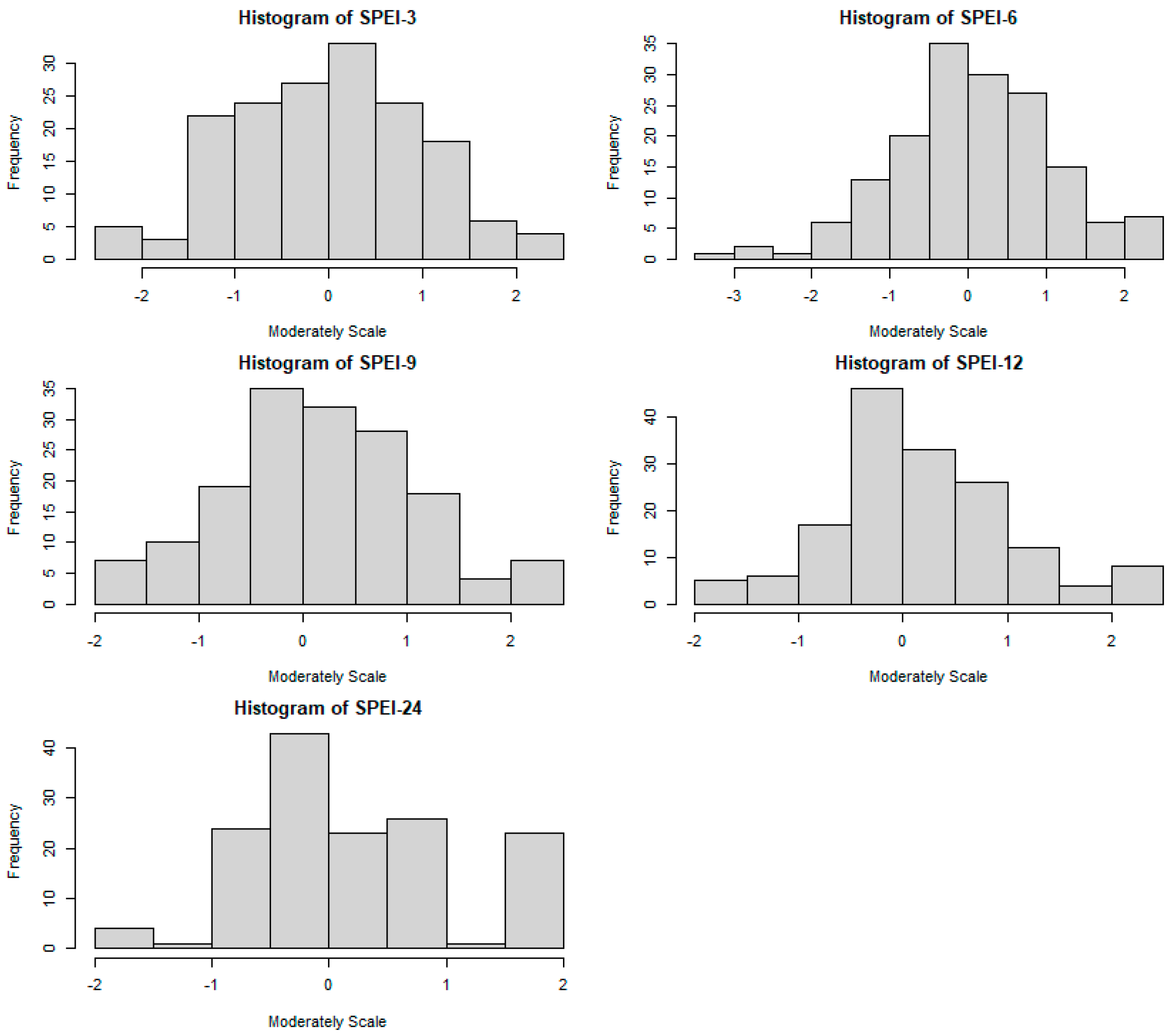
Figure 7 depicts the ACF and PACF of the residuals at various time scales. All the values of the ACF and PACF are found within the limit of 0.01 range for all lags. Thus, no significant association is found between residuals in Figure 8 and the normally distributed histograms of residuals for the SPEI at varying time scales have been represented. This result for the shaped model is sufficient for the SPEI time series data and residuals to error terms. The greatest accuracy predicting models linked to every examined SPEI time scale with accuracy fit measures (ME, RMSE, MAE, MPE, MAPE, MASE and Theil’s U) are shown in Table 14. In general, substantial results have been obtained for drought predicting with the help of ARIMA models in Tharparkar. In short explanation, the ARIMA models that have longer time scales shows profound ability of forecast and fit exactly with drought prediction in upcoming times.
Almost familiar results have been shown across world and put into the SPI that forms the core of SPEI, i.e., China [54] and India [35]. These research studies have shown that the time series of SPEI for Mithi, Tharparkar has the same nature as of Figure 3. In addition to this, the time series of SPEI-12 and -24 has a similar trend, and likewise for the time series of SPEI-3 and -6, respectively. The identical order seems to be for the time series depending on 12 and 24 months however, the related 3- and 6-month scale do not show this result.
From the Figure 5 for PACF and ACF it is clearly shown that the selected data is stationary.

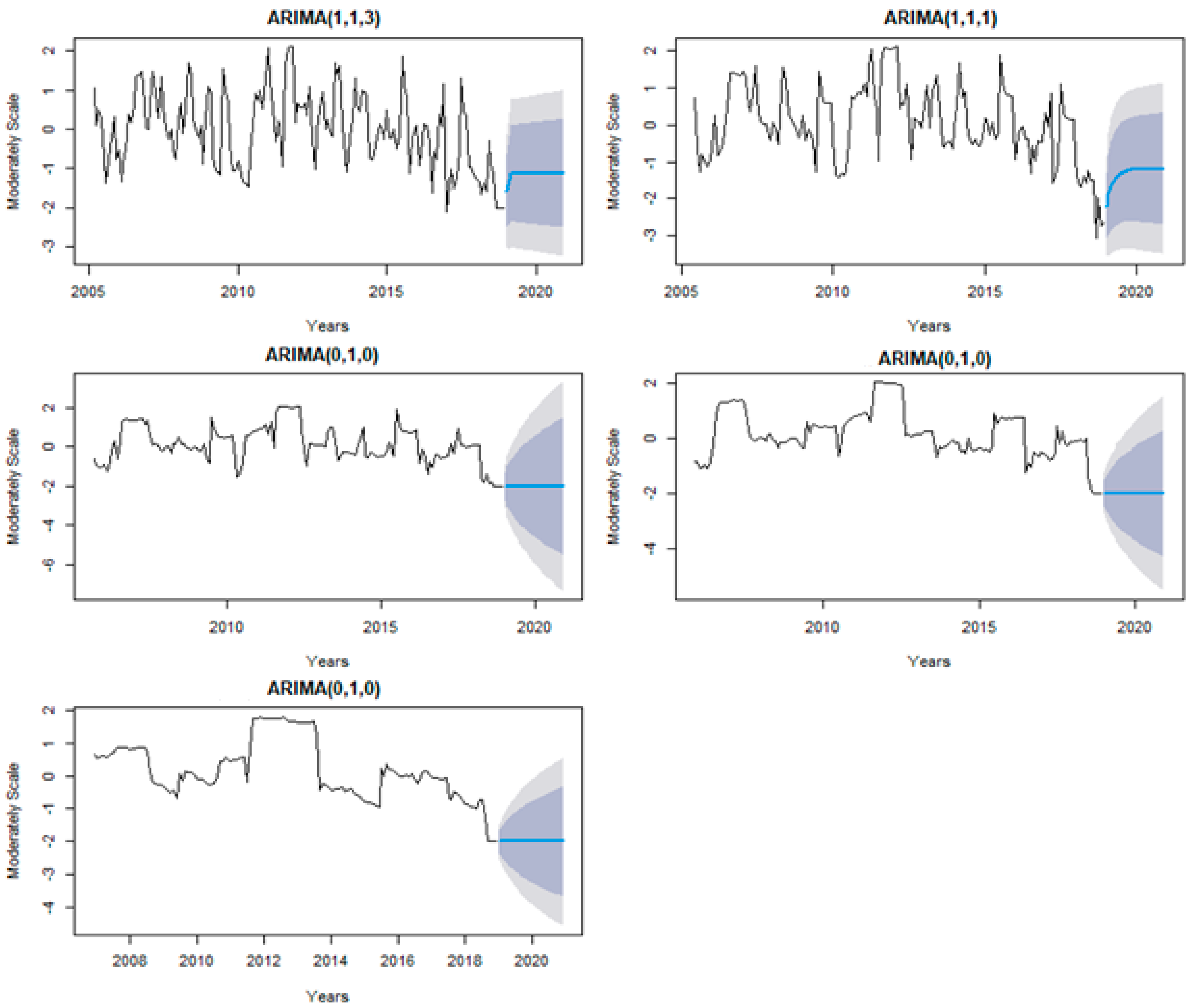
3.5. Model Forecasting

In fact, forecasting is one of the prime factors in decision making. It bears significant importance for the process about decision making and future planning. It assists in predicting the uncertain future by utilizing the behavior of past and ongoing experiments and observations. The forecasting that is performed using the ARIMA models lays out a sound basis for meteorological phenomena. The forecasting of drought is carried out by selecting the city of Tharparkar and then the data of that location has been utilized to foresee the data series of the SPEI at various time scales, from the 2005 to 2019 period to assess the agreement of data, where the examined and detected SPEI were plotted for its evaluation. Through the prism of comparison within predicted and observed data in Figure 9 and Figure 10, high authenticity of forecasted data is observed. No doubt, with the increase in number of SPEI time series, the forecasting ability of model will be improved. This enhancement in the ability of model is due to rising number of SPEI time series that filters the final values, resulting in the decline of sudden shifts in the curve of SPEI.
The comparison of A.R and M.A coefficients suggests that the ARIMA models of 24-month time scale for Tharparkar is quite accurate. ARIMA models of 3-month time scale are similar in the surrounding regions of Tharparkar. The ARIMA models of 24-month time scale also showed the very accurate results. In Table 7, Table 8, Table 9, Table 10, Table 11, Table 12 and Table 13, the estimation of like parameters of developed ARIMA model has been shown. From the outcome in Table 14, the value of p, d, q, P, D, and Q received from the models shaped for Tharparkar are almost alike at the same time scales. Hence, the ARIMA model (0,1,0), (1,0,2) at 24-SPEI could be summarized for the whole region of Tharparkar. In addition to this, the ARIMA model (1,1,3)(0,0,0) at 3-SPEI is also applicable to the neighboring cities of Tharparkar as they are very close to it. In Table 15, Table 16, Table 17, Table 18 and Table 19, the point forecasted values of SPEI-3, 6, 9, 12 and 24 for five years model has been shown.
For the (0,1,0)(1,0,2) model estimation, the series is stationary and prediction for this kind of series is the average of the series, model (0,1,0) whose A.R. term is 0, difference/order of integration is 1 and moving average is 0, and the (1,0,2) model who’s A.R has 1 lag, difference/order of integration is 0 and moving average has 2 lags.

3.6. Comparison with Previous Study

The comparative results of present and a previous study has been shown in Table 20. It is investigated that the present standard error and t-value of different SPEI (3, 6 and 24) have significant coherence with previous study [39].

4. Conclusions

This research proves SPEI as a unique and powerful multi-scalar drought index for the examination of drought event variations in the region of Tharparkar, Sindh. The prime objective of this research work is categorized into two parts. The first part deals with the evaluation of climatic parameters and drought frequency on the basis of SPEI. This research concluded that the water crisis are a result of overlapping of two unfavorable factors—a decrease in precipitation amounts and an increase of temperature in the region of Tharparkar. Therefore, due to the deficiency of water, the likelihood of drought events has been greatly increased such situation is ultimately generating immense threat to available water resources. In addition to this, the variation in SPEI also shows unusual course of drought (extremely dry) since preceding decade. However, from these results, it is also evident that the situation of hyper-arid regions could be more alarming and eye-opening. It should be noted that the forecast of drought events is one of the most troublesome issues faced be meteorologists.
In this way, the second objective of this research was related to the development and test of ARIMA models for the forecast of drought by utilizing SPEI with 3, 6, 9, 12, and 24-month time scales. The identification of the ARIMA models was conducted on the basis of AIC and SBC values. The basic point for researchers is the credibility of forecasted values. Because the implementation of drought alleviation policies depends upon these forecasted values. In this way, a series of diagnostic checking tests were conducted after the inspection of the parameters of said models. The ARIMA model (0,1,0)(1,0,2) at 24-SPEI could be selected from other possible models for the region of Tharparkar. Additionally, the ARIMA model (1,1,3)(0,0,0) at 3-SPEI, the ARIMA model (1,1,1)(0,0,2) at 6-SPEI, the ARIMA model (1,1,1)(1,0,0) at 9-SPEI and the ARIMA model (0,1,0)(1,0,2) at 12-SPEI can be generalized for Tharparkar region. This is because other localities are very close to the Mithi region. It was also observed that the result obtained through the ARIMA model at the 24-SPEI time scale was the best forecasting model, that follows the lower values of ME, RMSE, MAE, MPE, MAPE and MASE. The ARIMA model at SPEI 3-time scale was found to be the worst model for the prediction of drought for the region of Tharparkar. The best ARIMA models represent profound accuracy in foretelling the droughts, as these can perform a very significant role for planners and water resources managers in measures for such regions as well as in view of drought.
In fact, the connectivity between climate change shown in droughts and the present water resources in Tharparkar is the need of the hour. Thus, in the Tharparkar region, it is very important to overcome the forecasted drought conditions and this should be considered as a significant future study. Additionally, unfortunately the Tharparkar region in Pakistan has only one meteorological station located at Mithi, which is the limitation of our study. Therefore, this study can be extended using different models and a larger set of data in future.

Author Contributions

Conceptualization, P.K. and S.F.S.; Data curation, P.K. and L.K.; Formal analysis, S.F.S., M.A.U., L.K. and R.F.Z.; Methodology, P.K. and R.F.Z.; Project administration, S.F.S. and M.A.U.; Software, P.K., L.K. and R.F.Z. All authors have read and agreed to the published version of the manuscript.

Funding

This research was supported from the Higher Education Commission (HEC), Islamabad, Pakistan under the National Research Program for Universities (NRPU 6872).

Institutional Review Board Statement

Not applicable.

Informed Consent Statement

Not applicable.

Data Availability Statement

Data sharing not applicable.

Acknowledgments

Authors acknowledge the support of the Higher Education Commission (HEC), Islamabad, Pakistan and the Mehran University of Engineering and Technology, Jamshoro, Pakistan. This research was supported from the Higher Education Commission (HEC), Islamabad, Pakistan under the National Research Program for Universities (NRPU-6872).

Conflicts of Interest

The authors declare that they have no known competing financial interest or personal relationships that could have appeared to influence the work reported in this paper.

Nomenclature

ACFAutocorrelation Function
AICAkaike information criterion
ANNArtificial Neural Network
A.RAutoregressive
ARIMAAutoregressive Integrated moving Average
M.AMoving Average
MAEMean Absolute Error
MAPEMean Absolute Percentile Error
MASEMean Absolute Square Error
MEMean Error
MPEMean Percentile Error
PACFPartial Autocorrelation Function
PAIPalfai aridity index
PCPNprecipitation
PDSIPalme drought severity index
PETpotential evapotranspiration
RMSERoot Mean Square Error
SBCSchwarz’s Bayesian criterion
SPEIStandardized Precipitation Evapotranspiration Index
SPIStandardized precipitation index
SWSISurface water supply index
Symbols
Δ slope of vapor pressure
d order of difference
Rnsurface net radian
Gsoil heat flux density
γ psychometric constant
Tmean daily air temperature
U2the wind speed
essaturated vapor pressure
eaactual vapor pressure
ω Mean of the series
η t error terms
η t i MA error terms
α i Parameter of Moving average model
β i Parameter of Autoregressive model
Z t Time series
Z t i AR error terms
β ( C ) Polynomial
α ( C ) Polynomial
Φ p seasonal AR parameter of order P
Θ Q seasonal MA parameter of order Q
X m observed SPEI
X s predicted SPEI
x i predicted value
x ^ i actual value
d number of regular difference for Non-Seasonal Model
pAutoregressive Parameter for Non-Seasonal Model
qMoving Average Parameter for Non-Seasonal Model
Dnumber of regular difference for Seasonal Model
PAutoregressive Parameter for Seasonal Model
QMoving Average Parameter for Seasonal Model

References

  1. Boretti, A.; Rosa, L. Reassessing the projections of the World Water Development Report. NPJ Clean Water 2019, 2, 1–6. [Google Scholar] [CrossRef]
  2. Diffenbaugh, N.S.; Pal, J.S.; Trapp, R.J.; Giorgi, F. Fine-scale processes regulate the response of extreme events to global climate change. Proc. Natl. Acad. Sci. USA 2005, 102, 15774–15778. [Google Scholar] [CrossRef] [PubMed] [Green Version]
  3. Sheffield, J.; Wood, E. Projected changes in drought occurrence under future global warming from multi-model, multi-scenario, IPCC AR4 simulations. Clim. Dyn. 2008, 31, 79–105. [Google Scholar] [CrossRef]
  4. Berbel, J.; Esteban, E. Droughts as a catalyst for water policy change. Analysis of Spain, Australia (MDB), and California. Glob. Environ. Chang. 2019, 58, 101969. [Google Scholar] [CrossRef]
  5. Zandalinas, S.I.; Mittler, R.; Balfagón, D.; Arbona, V.; Gómez-Cadenas, A. Plant adaptations to the combination of drought and high temperatures. Physiol. Plant. 2018, 162, 2–12. [Google Scholar] [CrossRef] [Green Version]
  6. Madani, K.; AghaKouchak, A.; Mirchi, A. Iran’s Socio-economic Drought: Challenges of a Water-Bankrupt Nation. Iran. Stud. 2016, 49, 997–1016. [Google Scholar] [CrossRef]
  7. Marengo, J.A.; Alves, L.M.; Alvala, R.C.; A Cunha, A.P.M.; Brito, S.; Moraes, O. Climatic characteristics of the 2010-2016 drought in the semiarid Northeast Brazil region. Anais Acad. Bras. Cienc. 2018, 90, 1973–1985. [Google Scholar] [CrossRef]
  8. Montaseri, M.; Amirataee, B. Comprehensive stochastic assessment of meteorological drought indices. Int. J. Clim. 2017, 37, 998–1013. [Google Scholar] [CrossRef]
  9. Belayneh, A.; Adamowski, J. Drought forecasting using new machine learning methods. J. Water Land Dev. 2013, 18, 3–12. [Google Scholar] [CrossRef]
  10. Jesus, E.T.d.; Amorim, J.d.S.; Junqueira, R.; Viola, M.R.; Mello, C.R. Meteorological and Hydrological Drought from 1987 to 2017 in Doce River Basin, Southeastern Brazil; RBRH: Porto Alegre, Brazil, 2020; Volume 25. [Google Scholar]
  11. Vangelis, H.; Tigkas, D.; Tsakiris, G. The effect of PET method on Reconnaissance Drought Index (RDI) calculation. J. Arid. Environ. 2013, 88, 130–140. [Google Scholar] [CrossRef]
  12. Li, J.; Wang, Z.; Wu, X.; Xu, C.-Y.; Guo, S.; Chen, X. Toward Monitoring Short-Term Droughts Using a Novel Daily Scale, Standardized Antecedent Precipitation Evapotranspiration Index. J. Hydrometeorol. 2020, 21, 891–908. [Google Scholar] [CrossRef]
  13. Kwon, H.-J.; Kim, S.-J. Assessment of distributed hydrological drought based on hydrological unit map using SWSI drought index in South Korea. KSCE J. Civ. Eng. 2010, 14, 923–929. [Google Scholar] [CrossRef]
  14. Bucur, D.; Corduneanu, F.; Vintu, V.; Balan, I.; Crenganis, L. Impact of drought on water resources in North Eastern Romania. Case study—The prut river. Environ. Eng. Manag. J. 2016, 15, 1213–1222. [Google Scholar] [CrossRef]
  15. Kalisa, W.; Zhang, J.; Igbawua, T.; Ujoh, F.; Ebohon, O.J.; Namugize, J.N.; Yao, F. Spatio-temporal analysis of drought and return periods over the East African region using Standardized Precipitation Index from 1920 to 2016. Agric. Water Manag. 2020, 237, 106195. [Google Scholar] [CrossRef]
  16. Bong, C.H.J.; Richard, J. Drought and climate change assessment using Standardized Precipitation Index (SPI) for Sarawak River Basin. J. Water Clim. Chang. 2020, 11, 956–965. [Google Scholar] [CrossRef]
  17. Hoffmann, D.; Gallant, A.J.E.; Arblaster, J.M. Uncertainties in Drought from Index and Data Selection. J. Geophys. Res. Atmos. 2020, 125, 031946. [Google Scholar] [CrossRef]
  18. Anshuka, A.; Buzacott, A.J.V.; Vervoort, R.W.; van Ogtrop, F.F. Developing drought index–based forecasts for tropical climates using wavelet neural network: An application in Fiji. Theor. Appl. Clim. 2021, 143, 557–569. [Google Scholar] [CrossRef]
  19. Vicente-Serrano, S.M.; Beguería, S.; López-Moreno, J.I. A multiscalar drought index sensitive to global warming: The standard-ized precipitation evapotranspiration index. J. Clim. 2010, 23, 1696–1718. [Google Scholar] [CrossRef] [Green Version]
  20. Wainwright, H.M.; Steefel, C.; Trutner, S.D.; Henderson, A.N.; Nikolopoulos, E.I.; Wilmer, C.F.; Chadwick, K.D.; Falco, N.; Schaettle, K.B.; Brown, J.B.; et al. Satellite-derived foresummer drought sensitivity of plant productivity in Rocky Mountain headwater catch-ments: Spatial heterogeneity and geological-geomorphological control. Environ. Res. Lett. 2020, 15, 084018. [Google Scholar] [CrossRef]
  21. Zarei, A.R.; Shabani, A.; Moghimi, M.M. Accuracy Assessment of the SPEI, RDI and SPI Drought Indices in Regions of Iran with Different Climate Conditions. Pure Appl. Geophys. PAGEOPH 2021, 178, 1387–1403. [Google Scholar] [CrossRef]
  22. Li, L.; She, D.; Zheng, H.; Lin, P.; Yang, Z.-L. Elucidating Diverse Drought Characteristics from Two Meteorological Drought Indices (SPI and SPEI) in China. J. Hydrometeorol. 2020, 21, 1513–1530. [Google Scholar] [CrossRef]
  23. Bai, X.; Shen, W.; Wu, X.; Wang, P. Applicability of long-term satellite-based precipitation products for drought indices considering global warming. J. Environ. Manag. 2020, 255, 109846. [Google Scholar] [CrossRef]
  24. Hao, Z.; Singh, V.P.; Xia, Y. Seasonal Drought Prediction: Advances, Challenges, and Future Prospects. Rev. Geophys. 2018, 56, 108–141. [Google Scholar] [CrossRef] [Green Version]
  25. Rhee, J.; Im, J. Meteorological drought forecasting for ungauged areas based on machine learning: Using long-range climate forecast and remote sensing data. Agric. For. Meteorol. 2017, 237–238, 105–122. [Google Scholar] [CrossRef]
  26. Papacharalampous, G.; Tyralis, H.; Koutsoyiannis, D. Predictability of monthly temperature and precipitation using automatic time series forecasting methods. Acta Geophys. 2018, 66, 807–831. [Google Scholar] [CrossRef]
  27. Chen, P.; Niu, A.; Liu, D.; Jiang, W.; Ma, B. Time Series Forecasting of Temperatures using SARIMA: An Example from Nanjing. In IOP Conference Series: Materials Science and Engineering; IOP Publishing: England, UK, 2018. [Google Scholar]
  28. Hao, Z.; Hao, F.; Singh, V.P.; Ouyang, W.; Cheng, H. An integrated package for drought monitoring, prediction and analysis to aid drought modeling and assessment. Environ. Model. Softw. 2017, 91, 199–209. [Google Scholar] [CrossRef]
  29. Ozger, M. Significant wave height forecasting using wavelet fuzzy logic approach. Ocean Eng. 2010, 37, 1443–1451. [Google Scholar] [CrossRef]
  30. Hassanzadeh, Y.; Ghazvinian, M.; Abdi, A.; Baharvand, S.; Jozaghi, A. Prediction of short and long-term droughts using artificial neural networks and hydro-meteorological variables. arXiv 2020, arXiv:2006.02581. [Google Scholar]
  31. Ozger, M.; Mishra, A.K.; Singh, V.P. Estimating Palmer Drought Severity Index using a wavelet fuzzy logic model based on mete-orological variables. Int. J. Climatol. 2011, 31, 2021–2032. [Google Scholar] [CrossRef]
  32. Akinremi, O.O.; McGinn, S.M.; Barr, A. Evaluation of the Palmer Drought Index on the Canadian Prairies. J. Clim. 1996, 9, 897–905. [Google Scholar] [CrossRef] [Green Version]
  33. McKee, T.B.; Doesken, N.J.; Kleist, J. The relationship of drought frequency and duration to time scales. In Proceedings of the 8th Conference on Applied Climatology, Boston, MA, USA, 17–22 January 1993. [Google Scholar]
  34. Tian, M.; Wang, P.; Khan, J. Drought forecasting with vegetation temperature condition index using ARIMA models in the Guan-zhong Plain. Remote Sens. 2016, 8, 690. [Google Scholar] [CrossRef] [Green Version]
  35. Han, P.; Wang, P.; Tian, M.; Zhang, S.; Liu, J.; Zhu, D. Application of the ARIMA Models in Drought Forecasting Using the Standardized Precipitation Index. In Proceedings of the International Conference on Computer and Computing Technologies in Agriculture, Beijing, China, 18–20 September 2013. [Google Scholar]
  36. Shahzad, L.; Yasin, A. Analyzing Resilience and Food Insecurity of Drought Prone Communities of Tharparkar Desert. Available online: https://www.researchsquare.com/article/rs-472894/v1 (accessed on 21 September 2021).
  37. Memon, M.H.; Aamir, N.; Ahmed, N. Climate Change and Drought: Impact of Food Insecurity on Gender Based Vulnerability in District Tharparkar. Pak. Dev. Rev. 2018, 57, 307–321. [Google Scholar] [CrossRef] [Green Version]
  38. Pakistan Meteorological Department. PMD. Karachi. 1947. Available online: https://www.pmd.gov.pk/en/ (accessed on 21 September 2021).
  39. Mossad, A.; Alazba, A.A. Drought Forecasting Using Stochastic Models in a Hyper-Arid Climate. Atmosphere 2015, 6, 410–430. [Google Scholar] [CrossRef] [Green Version]
  40. Dikshit, A.; Pradhan, B.; Huete, A. An improved SPEI drought forecasting approach using the long short-term memory neural network. J. Environ. Manag. 2021, 283, 111979. [Google Scholar] [CrossRef]
  41. Agnew, C.T. Using the SPI to Identify Drought; University College London: London, UK, 2000. [Google Scholar]
  42. Valipour, M.; Banihabib, M.E.; Behbahani, S.M.R. Parameters estimate of autoregressive moving average and autoregressive in-tegrated moving average models and compare their ability for inflow forecasting. J. Math. Stat. 2012, 8, 330–338. [Google Scholar]
  43. Yuan, C.; Liu, S.; Fang, Z. Comparison of China’s primary energy consumption forecasting by using ARIMA (the autoregressive integrated moving average) model and GM (1, 1) model. Energy 2016, 100, 384–390. [Google Scholar] [CrossRef]
  44. Peiris, M.S.; Singh, N. Predictors for Seasonal and Nonseasonal Fractionally Integrated ARIMA Models. Biom. J. 1996, 38, 741–752. [Google Scholar] [CrossRef]
  45. Chang, Y.-W.; Liao, M.-Y. A Seasonal ARIMA Model of Tourism Forecasting: The Case of Taiwan. Asia Pac. J. Tour. Res. 2010, 15, 215–221. [Google Scholar] [CrossRef]
  46. Akaike, H. A new look at the statistical model identification. IEEE Trans. Autom. Control. 1974, 19, 716–723. [Google Scholar] [CrossRef]
  47. Mishra, A.K.; Singh, V.P. A review of drought concepts. J. Hydrol. 2010, 391, 202–216. [Google Scholar] [CrossRef]
  48. Makridakis, S.; Hibon, M. ARMA Models and the Box-Jenkins Methodology. J. Forecast. 1997, 16, 147–163. [Google Scholar] [CrossRef]
  49. Afrifa-Yamoah, E.; Mueller, U.; Taylor, S.M.; Fisher, A.J. Missing data imputation of high-resolution temporal climate time series data. Meteorol. Appl. 2019, 27, 1873. [Google Scholar] [CrossRef]
  50. RC Team. R: A Language and Environment for Statistical Computing. R Foundation for Statistical Computing. Available online: http://www.R-project.org/ (accessed on 15 July 2021).
  51. Mossad, A.; Mehawed, H.S.; El-Araby, A. Seasonal drought dynamics in El-Beheira governorate, Egypt. Am. J. Environ. Sci. 2014, 10, 140–147. [Google Scholar] [CrossRef] [Green Version]
  52. Sönmez, F.K.; Komuscu, A.U.; Erkan, A.; Turgu, E. An analysis of spatial and temporal dimension of drought vulnerability in Turkey using the standardized precipita-tion index. Nat. Hazards 2005, 35, 243–264. [Google Scholar] [CrossRef]
  53. Paulo, A.; Rosa, R.D.; Pereira, L.S. Climate trends and behaviour of drought indices based on precipitation and evapotranspiration in Portugal. Nat. Hazards Earth Syst. Sci. 2012, 12, 1481–1491. [Google Scholar] [CrossRef]
  54. Yu, M.; Li, Q.; Hayes, M.J.; Svoboda, M.; Heim, R.R., Jr. Are droughts becoming more frequent or severe in China based on the standardized precipitation evapotranspiration in-dex: 1951–2010? Int. J. Climatol. 2014, 34, 545–558. [Google Scholar] [CrossRef]
Figure 1. (a) Location of Pakistan in South Asia; (b) location of Tharparkar district in Pakistan. Both are highlighted with an arrow.
Atmosphere 12 01248 g001
Figure 2. Location of Mithi weather station (Meteorological Station); the data is collected for this station that was established in 2004.
Atmosphere 12 01248 g002
Figure 3. Time series plots of SPEI- 3, 6, 9, 12 and 24 are in right panel, and the left panel shows drought condition plots of SPEI- 3, 6, 9, 12 and 24.
Atmosphere 12 01248 g003
Figure 4. Precipitation and the highest rainfall during the period 2016 to 2019 and the lowest rain fall in the period of 2009 to 2014.
Atmosphere 12 01248 g004
Figure 5. Annual cycle of the precipitation the input data starts from 2004 to 2019.
Atmosphere 12 01248 g005
Figure 6. Annual cycle of the PET from 2004 to 2019 (Monthly variation).
Atmosphere 12 01248 g006
Figure 7. ACF and PACF of SPEI- 3, 6, 9, 12 and 24 from this we can identified the data is stationary.
Atmosphere 12 01248 g007
Figure 8. Residuals of SPEI- 3, 6, 9, 12 and 24 are normally distributed.
Atmosphere 12 01248 g008
Figure 9. The long-term projection of SPEI for 5 year.
Atmosphere 12 01248 g009
Figure 10. The long-term projection of SPEI for 30 years.
Atmosphere 12 01248 g010
Table 1. Ratio of drought in Colorado [33].
Drought ConditionRatio in Percentage
Mild24%
Moderate9.2%
Severe4.4%
Extreme2.3%
Table 2. SPEI scale [33,40,41].
ConditionsSPEI
DryExtremely SPEI 2
Severely 2 < SPEI 1.5
Moderately 1.5 < SPEI 1
NormalNear 1 < SPEI 1
WetModerately 1 < SPEI 1.5
Severely 1.5 < SPEI 2
Extremely SPEI 2
Table 3. Augmented Dickey–Fuller test.
SPEIDecisionp-Value of Unit Root at LevelUnit Root at 1st DifferenceUnit Root at 2nd Difference
SPEI-3No0.01N/AN/A
SPEI-6No0.01N/AN/A
SPEI-9No0.01134N/AN/A
SPEI-12No0.03514N/AN/A
SPEI-24Yes0.56350.01N/A
Table 4. Phillips–Perron unit root test.
SPEIDecisionp-Value of Unit Root at LevelUnit Root at 1st DifferenceUnit Root at 2nd Difference
SPEI-3No0.01N/AN/A
SPEI-6No0.01N/AN/A
SPEI-9No0.01N/AN/A
SPEI-12No0.09258N/AN/A
SPEI-24Yes0.55610.01N/A
Table 5. KPSS test for level stationarity.
SPEIDecisionp-Value of Unit Root at LevelUnit Root at 1st Difference
SPEI-3No0.1N/A
SPEI-6No0.1N/A
SPEI-9No0.1N/A
SPEI-12No0.1N/A
SPEI-24No0.0469N/A
Table 6. Seasonal ARIMA and non-seasonal ARIMA models.
Time ScalesSeasonal ARIMA ModelsNon-Seasonal ARIMA Models
SPEI-3ARIMA (1,1,3)(0,0,0)ARIMA (1,1,3)
SPEI-6ARIMA (1,1,1)(0,0,2)ARIMA (1,1,1)
SPEI-9ARIMA (1,1,1)(1,0,0)ARIMA (0,1,0)
SPEI-12ARIMA (0,1,0)(1,0,2)ARIMA (0,1,0)
SPEI-24ARIMA (0,1,0)(1,0,2)ARIMA (0,1,0)
Table 7. SPEI-3 ARIMA (1,1,3)(0,0,0) for Seasonal.
SPEI 3 CoefficientStandard Errort-Valuep-Value
A R t 1 −0.03920.2060−0.19029130.3912019
M A t 1 −0.26540.1910−1.3895290.15169
M A t 2 −0.20650.0991−2.0837540.04607481
M A t 3 −0.37570.1038−3.6194610.0006903546
Table 8. SPEI-3 ARIMA (1,1,3) for non-seasonal.
SPEI 3 CoefficientStandard Errort-Valuep-Value
A R t 1 −0.03920.2060−0.19029130.3912019
M A t 1 −0.26540.1910−1.3895290.15169
M A t 2 −0.20650.0991−2.0837540.04607481
M A t 3 −0.37570.1038−3.6194610.0006903546
Table 9. SPEI-6 ARIMA (1,1,1)(0,0,2) for seasonal.
SPEI 6 CoefficientStandard Errort-Valuep-Value
A R t 1 0.67000.08957.4860348.854317 × 10−12
M A t 1 −0.91510.0528−17.331441.045039 × 10−39
M A t 2 −0.26010.1105−2.3538460.02562977
M A t 3 −0.29320.1369−2.1417090.04085877
Table 10. SPEI-6 ARIMA (1,1,1) for non-seasonal.
SPEI 6 CoefficientStandard Errort-Valuep-Value
A R t 1 0.69390.08128.5455671.644041 × 10−14
M A t 1 −0.94560.0428−22.093461.130022 × 10−52
Table 11. SPEI-9 ARIMA (1,1,1)(1,0,0) for seasonal.
SPEI 9 CoefficientStandard Errort-Valuep-Value
A R t 1 0.80700.071711.255234.54369 × 10−22
M A t 1 −0.96190.0412−23.347096.873699 × 10−56
M A t 2 −0.15500.0825−1.8787880.06870885
Table 12. SPEI-12 ARIMA (0,1,0)(1,0,2) for Seasonal.
SPEI 12 CoefficientStandard Errort-Valuep-Value
A R t 1 0.39030.40200.97089550.2483222
M A t 1 −0.94330.4071−2.3171210.02786761
M A t 2 0.13350.25500.52352940.3471406
Table 13. SPEI-24 ARIMA (0,1,0)(1,0,2) for seasonal.
SPEI 24 CoefficientStandard Errort-Valuep-Value
A R t 1 0.12530.13560.92404130.2596008
M A t 1 −0.01250.1671−0.074805510.3972693
M A t 2 −0.73080.1208−6.0496692.116665 × 10−8
Table 14. Errors of SPEI-3, 6, 9, 12 and 24.
AccuracyMERMSEMAEMPEMAPEMASETheil’s U
SPEI-3 Test set−0.22740.85340.7261120.104120.1040.69720.9804
SPEI-6 Test set−0.78310.96480.8858117.805117.8050.85771.048
SPEI-9 Test set−0.49880.87470.7941100.101100.1010.79731.0798
SPEI-12 Test set−0.07841.0090.946291.84191.8410.96321.067
SPEI-24 Test set1.40861.41391.4086206.6870206.6871.99541.067
Table 15. Point forecasted value of SPEI-3 for five years.
Point Forecast
JanuaryFebruaryMarchAprilMayJuneJulyAugustSeptemberOctoberNovemberDecember
2019−1.05594−1.00396−0.97157−0.9729−0.9729−0.9729−0.9729−0.9729−0.9729−0.9729−0.9729−0.9729
2020−0.9729−0.9729−0.9729−0.9729−0.9729−0.9729−0.9729−0.9729−0.9729−0.9729−0.9729−0.9729
2021−0.9729−0.9729−0.9729−0.9729−0.9729−0.9729−0.9729−0.9729−0.9729−0.9729−0.9729−0.9729
2022−0.9729−0.9729−0.9729−0.9729−0.9729−0.9729−0.9729−0.9729−0.9729−0.9729−0.9729−0.9729
2023−0.9729−0.9729−0.9729−0.9729−0.9729−0.9729−0.9729−0.9729−0.9729−0.9729−0.9729−0.9729
Table 16. Point forecasted value of SPEI-6 for five years.
Point Forecast
JanuaryFebruaryMarchAprilMayJuneJulyAugustSeptemberOctoberNovemberDecember
2019−2.19456−1.88657−1.67284−1.52453−1.42161−1.35019−1.30063−1.26624−1.24237−1.22581−1.21432−1.20635
2020−1.20081−1.19697−1.19246−1.19118−1.19029−1.18967−1.18924−1.18894−1.18874−1.18874−1.18859−1.18849
2021−1.18842−1.18838−1.18834−1.18832−1.1883−1.18829−1.18828−1.18828−1.18828−1.18827−1.18827−1.18827
2022−1.18827−1.18827−1.18827−1.18827−1.18827−1.18827−1.18827−1.18827−1.18827−1.18827−1.18827−1.18827
2023−1.18827−1.18827−1.18827−1.18827−1.18827−1.18827−1.18827−1.18827−1.18827−1.18827−1.18827−1.18827
Table 17. Point forecasted value of SPEI-9 for five years.
Point Forecast
JanuaryFebruaryMarchAprilMayJuneJulyAugustSeptemberOctoberNovemberDecember
2019−2−2−2−2−2−2−2−2−2−2−2−2
2020−2−2−2−2−2−2−2−2−2−2−2−2
2021−2−2−2−2−2−2−2−2−2−2−2−2
2022−2−2−2−2−2−2−2−2−2−2−2−2
2023−2−2−2−2−2−2−2−2−2−2−2−2
Table 18. Point forecasted value of SPEI-12 for five years.
Point Forecast
JanuaryFebruaryMarchAprilMayJuneJulyAugustSeptemberOctoberNovemberDecember
2019−2−2−2−2−2−2−2−2−2−2−2−2
2020−2−2−2−2−2−2−2−2−2−2−2−2
2021−2−2−2−2−2−2−2−2−2−2−2−2
2022−2−2−2−2−2−2−2−2−2−2−2−2
2023−2−2−2−2−2−2−2−2−2−2−2−2
Table 19. Point forecasted value of SPEI-24 for five years.
Point Forecast
JanuaryFebruaryMarchAprilMayJuneJulyAugustSeptemberOctoberNovemberDecember
2019−1.90309−1.90309−1.90309−1.90309−1.90309−1.90309−1.90309−1.90309−1.90309−1.90309−1.90309−1.90309
2020−1.90309−1.90309−1.90309−1.90309−1.90309−1.90309−1.90309−1.90309−1.90309−1.90309−1.90309−1.90309
2021−1.90309−1.90309−1.90309−1.90309−1.90309−1.90309−1.90309−1.90309−1.90309−1.90309−1.90309−1.90309
2022−1.90309−1.90309−1.90309−1.90309−1.90309−1.90309−1.90309−1.90309−1.90309−1.90309−1.90309−1.90309
2023−1.90309−1.90309−1.90309−1.90309−1.90309−1.90309−1.90309−1.90309−1.90309−1.90309−1.90309−1.90309
Table 20. A comparison of the present and previous study [39].
SPEIStandard Error of Previous Studyt-Value of Previous StudyStandard Error of Present Studyt-Value of Present Study
3 AR0.1055.840.2060−0.1902913
3 MA0.117−3.270.1910−1.38925
0.104−3.460.0991−2.083754
0.0942.430.1038−3.619461
6 AR0.0547.540.08957.486034
6 MA0.048−15.490.0528−17.3314
0.054−12.010.1105−2.353846
0.052−9.990.1369−2.141709
0.043−11.30
0.033−16.74
24 AR0.0366.980.13560.9240413
24 MA0.048−7.470.1671−0.07480551
0.034−14.540.1208−6.049669
Publisher’s Note: MDPI stays neutral with regard to jurisdictional claims in published maps and institutional affiliations.

