Article

Evaluation of Historical CMIP6 Model Simulations of Seasonal Mean Temperature over Pakistan during 1970–2014

1
Collaborative Innovation Center on Forecast and Evaluation of Meteorological Disasters/Key Laboratory of Meteorological Disaster, Ministry of Education, Nanjing University of Information Science and Technology, Nanjing 210044, China
2
Jiangsu Key Laboratory of Atmospheric Environment Monitoring and Pollution Control, Collaborative Innovation Centre of Atmospheric Environment and Equipment Technology, School of Environmental Science and Engineering, Nanjing University of Information Science and Technology, Nanjing 210044, China
3
Binjiang College of Nanjing University of Information Science and Technology, Wuxi 214000, China
4
School of Atmospheric Sciences and Guangdong Province Key Laboratory for Climate Change and Natural Disaster Studies, Sun Yat-sen University, Zhuhai 519082, China
5
Southern Marine Science and Engineering Guangdong Laboratory (Zhuhai), Zhuhai 519082, China
*
Author to whom correspondence should be addressed.
Atmosphere 2020, 11(9), 1005; https://doi.org/10.3390/atmos11091005
Submission received: 20 July 2020 / Revised: 11 September 2020 / Accepted: 16 September 2020 / Published: 20 September 2020
(This article belongs to the Special Issue Climate Events and Extreme Weather)

Abstract

:
This work employed recent model outputs from coupled model intercomparison project phase six to simulate surface mean temperature during the June–July–August (JJA) and December–January–February (DJF) seasons for 1970–2014 over Pakistan. The climatic research unit (CRU TS4.03) dataset was utilized as benchmark data to analyze models’ performance. The JJA season exhibited the highest mean temperature, whilst DJF displayed the lowest mean temperature in the whole study period. The JJA monthly empirical cumulative distribution frequency (ECDF) range (26 to 28 °C) was less than that of DJF (7 to 10 °C) since JJA matched closely to CRU. The JJA and DJF seasons are warming, with higher warming trends in winters than in summers. On temporal scale, models performed better in JJA with overall low bias, low RMSE (root mean square error), and higher positive CC (correlation coefficient) values. DJF performance was undermined with higher bias and RMSE with weak positive correlation estimates. Overall, CanESM5, CESM2, CESM2-WACCM, GFDL-CM4, HadGEM-GC31-LL, MPI-ESM1-2-LR, MPI-ESM1-2-HR, and MRI-ESM-0 performed better for JJA and DJF.

1. Introduction

The surface temperature increase has placed scientists on alert since the post-industrial era for its harmful impacts on the earth’s ecosystems and human welfare in general. The average warming rate over land has increased by 0.72 °C since 1951 and may increase further by 1.8 to 4 °C by the end of the 21st century [1]. Changes in climate mechanisms, like an increase in temperature, have a considerable impact on hydrology, ecology, and socioeconomics in the form of floods, droughts, heatwaves, and a decrease in low-temperature magnitude and frequency [2,3]. South Asia is the most vulnerable to climate change, under temperature increase, threatening one fourth (1.8 billion) of the global population [4,5]. Rapidly melting Himalayan glaciers under noticeable warming rates, variability in seasonal precipitation, and frequency of extreme events have damaged the economy, agriculture, livelihoods, infrastructure, and general welfare of this region [6].
Pakistan’s climate is changing rapidly as of 2020; it stands as the eighth most vulnerable country to climate change impacts and aftermath [7]. The nation’s economic backbone, agriculture, depends on glaciers and rainfall for commercial, domestic, and agricultural activities [8]. The glaciers of Hindu Kush, Himalayas, and Karakorum are melting rapidly under global warming, further deteriorating the population anguishes by triggering floods, glacial lake outburst floods, land erosion, infrastructure damage, and loss of human lives [9]. From 1901 to 2007, the area-weighted mean temperature over Pakistan was recorded as 0.64 °C, and it is constantly increasing at 0.06 °C/decade [10].
Summer and winter are hydrologically the most important seasons in Pakistan, where most (51–80%) of country water needs are met in the form of rain and snow [11]. Researchers found recently that most of the temperature changes and variability occurred during summer and winter seasons. The minimum temperatures in winters are rising rapidly (0.17–0.37 °C/decade) compared to the summer temperature (which is maximum) over Pakistan [12]. For instance, Ullah et al. [13] observed maximum warming rates (0.22 and 0.33 °C/decade for Tmax and Tmin) during winter and summer (0.20 and 0.25 °C/decade) seasons over Pakistan. Further, Adnan et al. [14] observed maximum temperature during June–July–August (JJA) and minimum temperature during December–January–February (DJF), with the increase in winter minimum temperatures in recent years. The temperature intensity and frequency dynamics with spatiotemporal changes may lead to surface warming, droughts, and heatwaves; under changes in land cover, deforestation, and other human activities [15]. Pakistan, since recent times, is under a warming trend, with a rapid increase in temperature over northern and southwestern mountainous regions, largely due to snow/ice-albedo feedback mechanism, and other factors [16]. Factors like vegetation cover, topography, cloud cover, urbanization scale, land-use change, agricultural practices, industrialization, and others may influence temperature through direct and indirect mechanisms [15,16,17]. The significant cold extremes are warming faster than the warm extremes, over higher latitudes, and altitudes under polar amplification and snow-albedo feedback processes; land surface extremes warm faster than air temperature for the same period [18]. According to [12,19,20,21], the mean temperature manifests the average change and trends in extremes of temperature, i.e., Tmax and Tmin. This link can be useful in understanding and predicting future trends of extreme weather events. Moreover, the Tmean trend changes may be due to changes in either Tmax or Tmin or both [4].
Climate models are fundamental tools to acquire past and future climate information through utilization of estimation techniques for the land, ocean, atmosphere, and ice interactions [22]. General circulation models (GCMs) involve complex mathematical equations and physics, resulting in simulations at various spatiotemporal scales of a day to centuries [23]. The CMIP6 models are the latest generation of the Climate Models Intercomparison Project (CMIP), formulated around three specific scientific questions for earth response to forcings, the origin of the models’ systematic biases and errors, and understanding future climate amidst the internal variability, predictability, and uncertainties. The scientific backdrop of CMIP6 is the seven grand scientific challenges covering climate change dimensions under varying spatiotemporal scales. The CMIP6 has a federated structure with a large number of experiments, uniquely designed. Each CMIP6-endorsed model intercomparison project (21 MIPS) covers unique climate themes. The diagnostic, evaluation, and characterization of Klima (DECK) experiments and historical simulations are developed under different forcings scenarios of past climates. The five newly developed future scenarios of CMIP6, i.e., shared socioeconomic pathways (SSPs), follow the pre-industrial and CO2 forcings of CMIP5-RCPs with new forcings included subsequent to industrial, socioeconomic policy, technological, and human-induced impacts on the climate [24,25,26].
The CMIP6 models exhibit higher sensitivity to greenhouse gases (GHG) emissions compared to CMIP5 [27]. Grose et al. [26] observed CMIP6 has improved aerosols’ effect, models’ resolution, parameterization schemes, and more earth system models included. CMIP6 differs from CMIP5 with higher model climate sensitivity to GHG concentrations, contribution of different aerosols in GHGs, and aerosol forcing-based scenarios. New generation models provide improved temperature simulations under development of model resolution, intricate topography, atmosphere–biosphere transitions, and other features [28]. Higher climate sensitivity in CMIP6 causes overestimations in warming trends, and further carrying biases in future projections as well. Utilizing recalibrated/constrained models, robust use of ensembles based on process links, use of past trends, and climatology for current observation and consistent future projections are recommended procedures against biases. The high equilibrium climate sensitivity models better access the earth system behavior at higher levels of warming to estimate increase in extreme events [29].
Future climate changes can be predicted efficiently when past changes are observed well. [30]. CMIP6 historical simulations give forced (control) and unforced variability of climate, accessed through benchmarking common observations datasets against models. The CO2 emissions and concentration-driven forcings are embedded under pre-industrial control with additional estimated-historical runs to calibrate the CO2 forcings’ magnitude to a true level. Historical simulations give variability on the timescale from one day to several centuries because of close interactions of earth system components. Multi-model ensembles evidently identify signals of interest, since averaging the models’ members also averages/spreads the natural variability. In the case of such variability, the members’ spread around the average is due to unforced internal variability [24,31].
Limited studies have focused on the mean temperature variability across Pakistan under CMIP models. Almazroui et al. [27] observed a significant increase in warming for the 1995–2014 period over Pakistan. The highest annual mean temperature was over Southern Pakistan, while the near future (2030–2049) warming rate (1.1 for SSP1-2.6, 1.2 for SSP2-4.5, and 1.5 °C for SSP5-8.5) showed an increase in temperature, especially over the northern regions of Pakistan. Likewise, Ather and Latif [32] studied inter-seasonal temperature variability over Pakistan using CMIP3 and CMIP5 models; they observed temperature ranges of −15 to 25 °C in DJF, 25 to 30 °C in Mar–Apr–May, 25 to 35 °C in JJA, and −15 to 15 °C in Sep–Oct–Nov for the 1951–2000 period. Further, the JJA higher temperature band in the south stretched the impacts to the north, though in SON, the band retreated. The models (CM2.0, CM2.1, CM2p1, and CM3.0) performed overall good for temperature simulations. Further, Ali et al. [33] also studied historical simulations and statistically downscaled projections, and observed the average temperature warmed up at a rate of up to 0.5 °C for 1976–2005 for the entire Pakistan. The mean temperature gave an increasing trend, although some northern patches showed negative trends and model errors. Further, Sajjad and Ghaffar [34] studied historical and future extremes indices through CMIP5 models for 1960–2013. A significant rise (1.5 to 1.1 °C) in mean maximum temperature was observed over the northern regions of Pakistan. The northwestern regions (Khyber Pakhtun Khwa province) showed an increase of 0.9 °C in the mean maximum for 1960–2013. The central regions (Punjab and Baluchistan) showed an increasing trend (1.9 °C), particularly the mean minimum temperature. Southeastern (Sindh province) regions showed an increasing trend (1.6 °C) in both the maximum and the minimum temperatures. The southwest regions (Baluchistan) showed an increase of 1.8 °C for mean maximum temperature and 1.9 °C for mean minimum temperature. A study by Babar et al. [35] showed the historical climatic research unit (CRU) annual mean temperature of 16.54, 24.59 for summer, and 7.26 °C for winter; the University of Delaware (UDEL) dataset displayed summer mean temperatures of 16.40, 24.55, and 6.94 °C in winter. The CMIP5 multi-model ensemble gave summer mean temperatures of 15.24, 24.50, and 5.03 °C, respectively, in winter over Pakistan. Many models displayed cold bias, particularly over the northern regions, probably owing to the models’ inability to reproduce cloud properties, their coarser resolution, and the snow-albedo mechanism over the region.
This study emphasized CMIP6 models’ simulations and performance evaluations for 1970–2014 mean temperature, which is pertinent to climate change-focused researchers and stakeholders. Quantifying simulations and uncertainties are vital in understanding models’ reliability in determining future temperature trends under climate change [36]. Models’ performances vary considerably, and a reliable multi-model ensemble construct for the future requires strong evaluations [37]. The statistical downscaled products such as CORDEX (https://cordex.org/) do not change bias unless bias correction is applied on models to resolve model spread [38]. The remaining part of the paper is arranged as follows: Section 2 provides models and observation used and methods; Section 3 provides the results and discussion, while Section 4 gives a conclusion drawn from the findings.

2. Materials and Methods
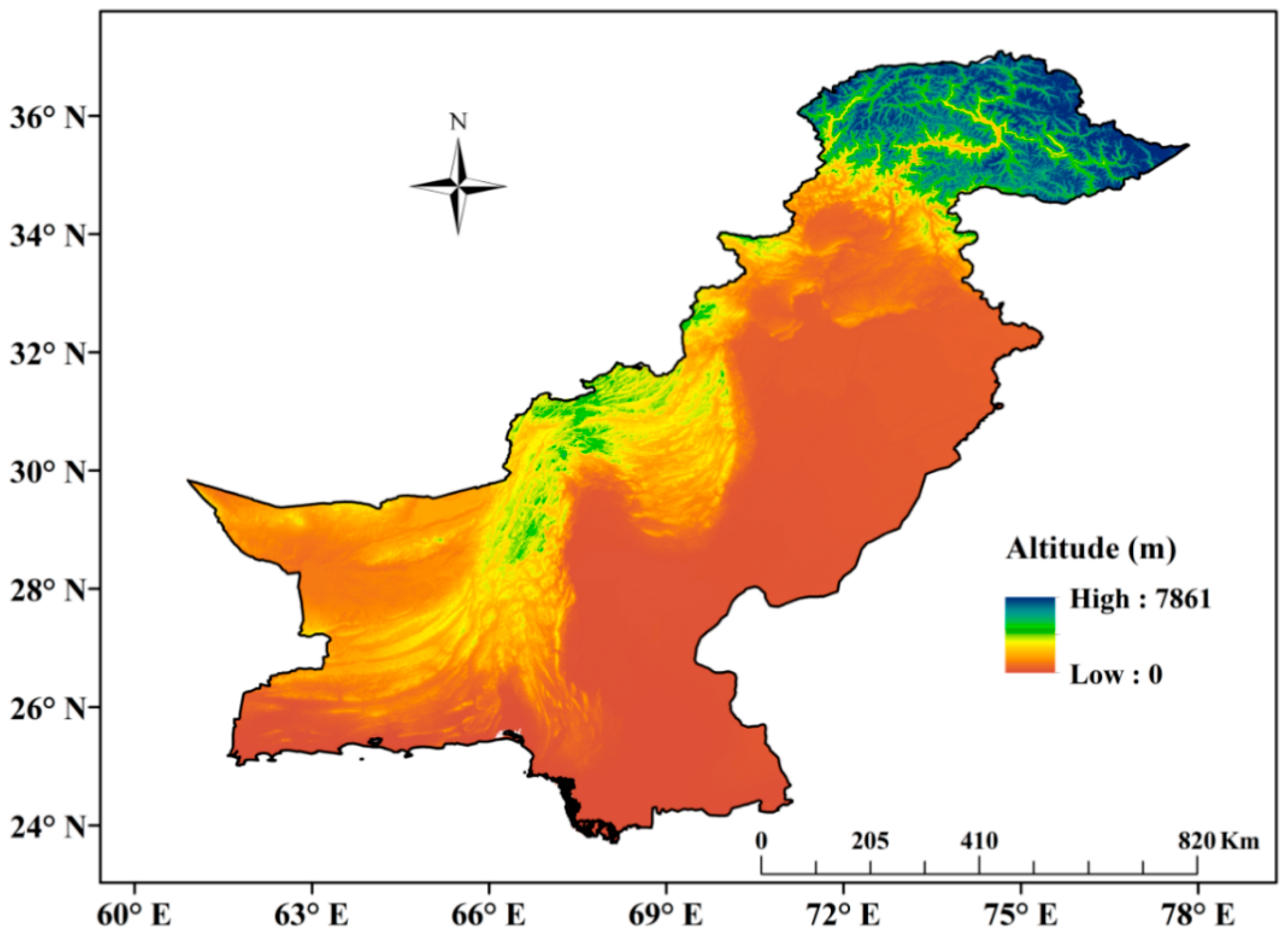
2.1. Study Area

Pakistan is situated in South Asia, extending between 23–37.5° N latitudes and 61–78° E longitudes (Figure 1) and covering an area of 880,940 km2. China borders it in the north, India in the east, Afghanistan and Iran in the west, and the Arabian Sea in the south. It features diverse geography such as the world’s highest mountainous regions (K2 peak-8200 m) in the north and northwest, to sea levels of 0 m at the Arabian Sea in the south. The central areas consist of the Indus Plains of Punjab and Sindh, while deserts are spread in the southeast and hyper-arid lands in the southwest [39].
The overall climate is arid (60% areas), featuring hot summers prominently across southern parts and cold winters in portions of northern humid Himalayan foothills (northeast and west) and northern mountains. The central regions have semi-arid to arid features, while coastal areas retain a unique coastal climate [40,41]. Summers are hot while winters are cold across the country; however, for a few past years, winters have been warming faster than summers [42].

2.2. Data and Methods

This study utilized thirteen CMIP6 climate models (Table 1), mainly covering the 1970–2014 period (https://esgf-node.llnl.gov/search/cmip6) for historical seasonal (JJA and DJF) mean near-surface temperature (tas) simulations over Pakistan. The 1970–2014 timescale was chosen since it is considered the new climatological normal for Pakistan, particularly in temperature change [13,16]. At first, each model’s single members were acquired from first members (member_id = r1i1p1f1) for each model by averaging members’ ensembles from 1970 through 2014. Next, models were treated for standard date format, standard variable unit, and common temporal length to get uniformed interpretable simulations. The model outputs were regridded to a common grid of 1.4 × 1.4° resolutions using the nearest neighbor interpolation technique. The nearest neighbor interpolation allowed better classification of similar close points by weighted average using data triangulation [43]. The land surfaces, particularly hilly terrains, were better interpolated due to sub-regionalization of grid points by the nearest cell center of an input grid [44]. The multi-model ensemble (MM-Ensemble) was created by simple averaging of regridded models for each season, i.e., summer and winter seasons; MM-Ensemble was preferred and believed to contain information from all models [45]. Regridded data were converted into monthly and then to respective seasonal scales. The CRU [46] mean temperature data was utilized as the benchmark for quantifying model simulations performance for summer and winter following [27].
The historical mean climatology of available CMIP6 models and CRU was plotted for summer and winter season. Further, the spatial and temporal performance of each model and MM-Ensemble simulation for seasonal mean simulations against CRU seasonal observations for 1970–2014 was in detail assessed by computing statistical metrics of bias; root mean square error (RMSE), and correlation coefficient (CC). The mathematical procedure of the above metrics was referenced from the following equations [47,48]:
B = 1 n k = 1 n ( M i O i )
C C = k = 1 n ( O i O i ¯ ) ( M i M l ¯ ) k = 1 n ( O i O i ¯ ) 2   k = 1 n ( M i O M l ¯ ) 2  
R M S E = 1 n k = 1 n ( M i O i ) 2
where M is model-simulated and O is observed values series, i refer to observed and simulated pairs, while n is the total number of pairs.
Reliable future projections depend on the accurate picture of the mean climate and past climate trends. The temporal trends in observed and simulated climatology were detected using the Mann–Kendall (MK) trend test [49,50]. The Mann–Kendall test is commonly used in numerous time-series trend studies [9,13,27,51]. This method exempts datasets from normal distribution requirements to handle outliers and missing values [13,49]. The MK test hypothesis states that the trend does not exist (H0), and the trend does exist (H1) in a time series. MK correlation coefficient/Kendall’s Tau establishes trends in time series. The strength of the trend is proportional to the magnitude of the MK test statistic, where greater magnitude exhibits stronger trends and lesser magnitudes show a weaker trend.
Trend test statics S is defined as:
S = i = 1 n 1 j = i + 1 n s g n ( x j x i )  
where x1, x2..xn represent n data points, xj represents the data point at jth time. Positive S indicates an increasing trend while low S value exhibits decreasing trends, i.e.:
s g n ( x j x i ) = { f o r ( x j x i ) > 0 f o r ( x j x i ) = 0 f o r ( x j x i ) < 1 }    
where xj and xi represent the time series observations, and n is length of the time series. When n ≥ 10, the S is approximately independently distributed data with the mean of 0 is with a variance given as:
V a r ( S ) = n ( n 1 ) ( 2 n + 5 ) i = 1 m t i ( t i 1 ) ( 2 t i + 5 ) 18    
where n is number of data points, m is number of tied groups (a tied group is a set of sample data having the similar value), and ti is number of data points in the ith group. MK test statistic, Z, is computed as:
Z =   { S 1 V a r ( S ) 0 S + 1 V a r ( S ) } { i f   S > 0 i f   S = 0 i f S < 0 }      
If Z values remain beyond the confidence level of ±1.96, it shows a statistically significant trend at the 95% confidence level. The trend is considered decreasing if Z is negative and vice-versa. In this study, this method was applied to seasonal and annual (temporal only) time-series data. Moreover, Sen’s slope (SE) computes trend slope in time series [13,40,49]. For an existing linear trend in a time series, slope estimates of n pairs of data can be computed using the relation:
t i = x j x i j i      
where xj and xi represent data values at time j and i, while (j > i).
The median of the N values of Ti is considered as Sen’s estimator of slope, calculated as:
Q i = { T N + 1 2 1 2 ( ( T   N 2 + T   N + 2 2 ) }   { N = O d d N = E v e n }  
Positive Qi exhibits an increasing trend, while negative shows decreasing trends. For odd N, the upper part of Equation (9) is used to get SE, and for odd N, the lower part of the equation is used. Further, the true slope is obtained by applying a two-sided t-test on Qi at a 100% (1-α) confidence interval. Time series data on seasonal and annual scale was treated with MK and Sen’s slope estimator.
Further, the cumulative distribution function (F(x)) was used to fit different theoretical distributions of models’ simulations and compare them with the ones from observed patterns, to determine models’ symmetries deviating from observed patterns [40,48]. The raw model data was initially sorted, standardized, and processed in the high-performance computing (HPC) platform of Nanjing University of Information Science and Technology. Python, MATLAB, and few other open source software were utilized to analyze the datasets and plot the outputs in this work.

3. Results

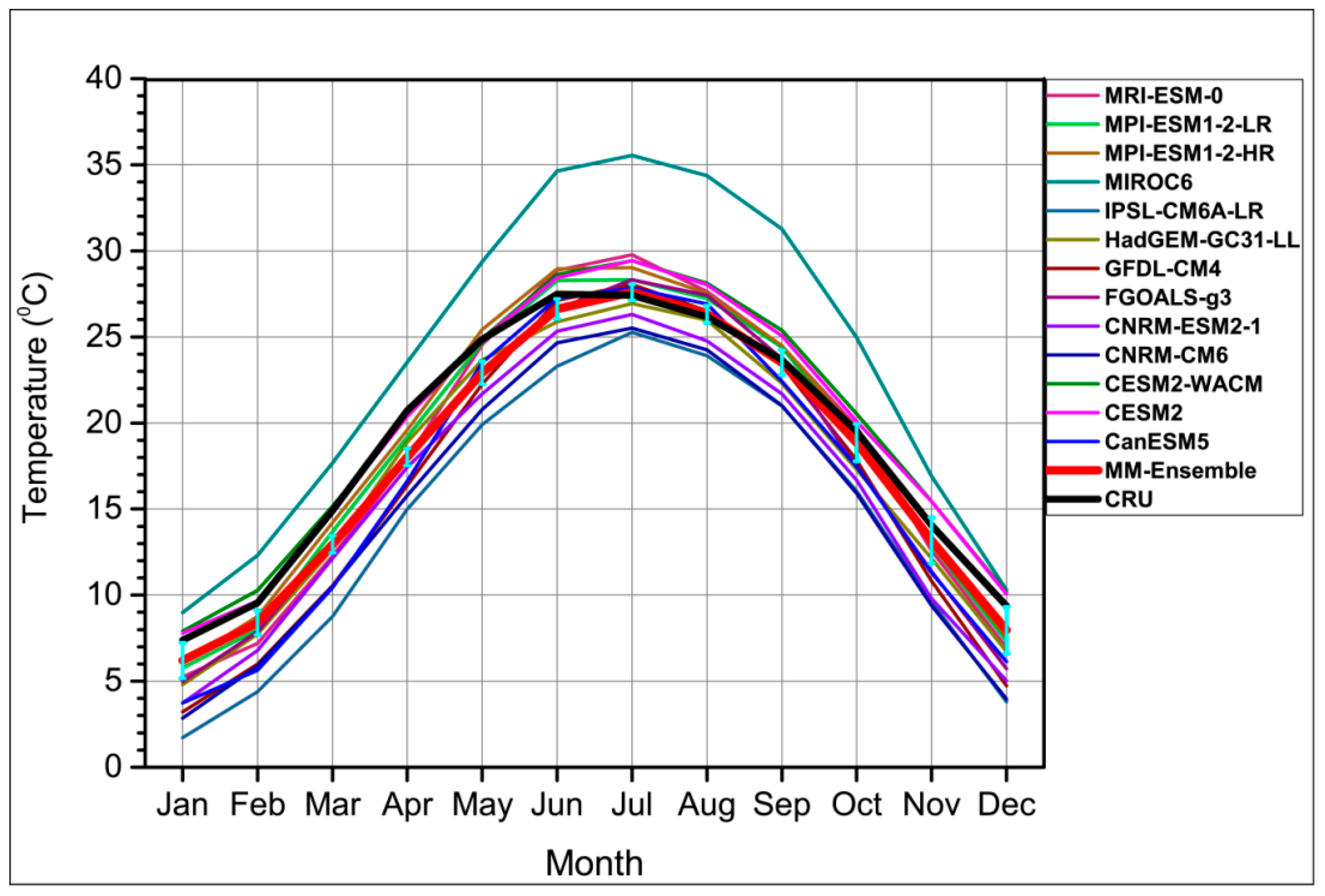
3.1. Mean Temperature Annual Cycle

The annual mean temperature cycle over Pakistan for 1970–2014 is shown in Figure 2. All the datasets display a bell-shaped distribution of mean temperature in the yearly cycle. A model is said to underestimate temperature when it simulates temperature values lower than the observed dataset; and vice versa in overestimation (higher values than observed patterns) of temperature. The CRU showed the annual highest mean temperatures during summer (JJA) and lowest mean temperatures during the winter (DJF) season. The months of June, July, and August exhibited 27 °C, 26 °C, and 25 °C temperatures, respectively, while December, January, and February showed 9 °C, 7 °C, and 9 °C. The MM-Ensemble, CESM2, CESM2-WACM, and MRI-ESM0 were consistent with CRU patterns. MIROC6, however, highly overestimated temperatures in April–October, while IPSL-CM6A-LR highly underestimated temperatures throughout the cycle. For summer (JJA) and winter (DJF), both interestingly displayed the maximum and minimum mean temperatures in the annual cycle. Overall, most of the models and MM-Ensemble simulations (except CNRM-ESM2-1, MIROC6, and IPSL-CM6A-LR) were consistent with CRU for all months. The December–March seasons show the highest underestimations, and May–November displayed the highest overestimations. Summer displayed annual maximum, while winter showed annual minimum temperatures. Previous works observed [20,52] that global circulation patterns influence temperatures of certain months or seasons (winter and summer season months by North Atlantic oscillations) with their contribution to winds, convection, diversion, and through dynamical thermal effects, henceforth, changing temperature magnitudes across this region.

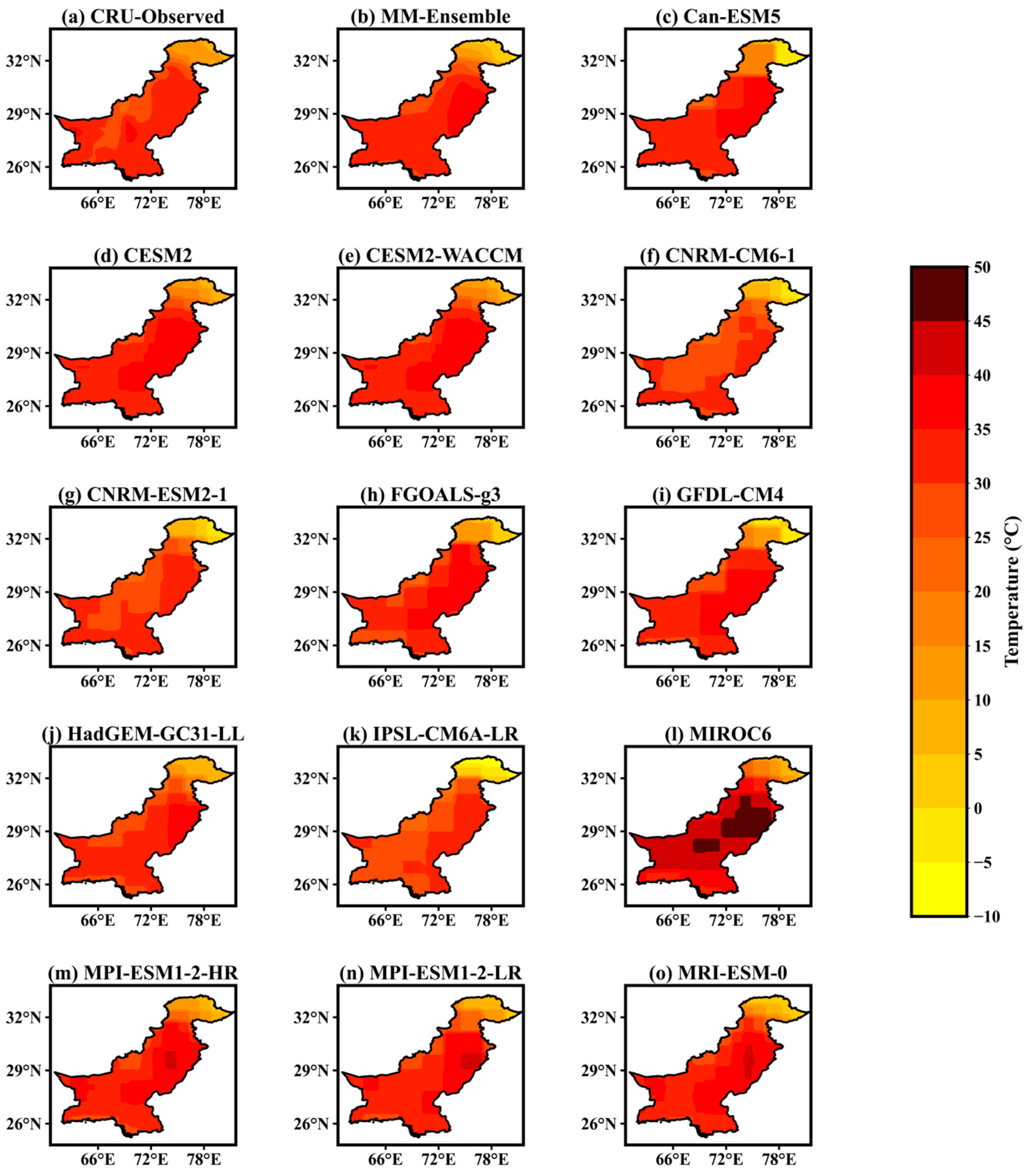
3.2. Summer Mean Temperature Climatology

The summer (JJA) mean temperature climatology patterns and simulations for 1970–2014 are plotted (Figure 3) over Pakistan. CRU patterns show the mean temperature in the range of 30 to 35 °C across southeastern, southern, and southwestern parts. Central-western regions exhibit a temperature of 25 °C to 30 °C and 5 to 20 °C over northern parts. The majority of models simulated north-south temperature dipole with high temperatures (20 °C to >35 °C) over central to southern regions and colder over the north. MM-Ensemble, Can-ESM5, CESM2, CESM2-WACCM, FGOALS, GFDL-CM4, and MRI-ESM-0 replicated CRU temperature over central-east, southeast, southwest, and western sides; some models also underestimated temperature over these regions. When compared to other models, MIROC6 highly overestimated temperature over the central to southern parts of Pakistan. Over northern regions, MM-Ensemble, CESM2, CESM2-WACCM, FGOALS-g3, and MIROC6 showed nearly consistent simulations with CRU patterns, and other models overestimated observed patterns. Overall, MM-Ensemble, CNRM-CM6-1, CNRM-ESM2-1, HadGEM-GC31-LL, MPI-ESM-2-HR, and MRI-ESM-0 models were consistent with CRU patterns (5 °C –35 °C) over the whole country. A study by [53] showed similar results with cold and warm bias over the northern and central regions of Pakistan, displaying a dipole pattern with higher temperatures over southern parts and relatively lowers at higher latitudes.

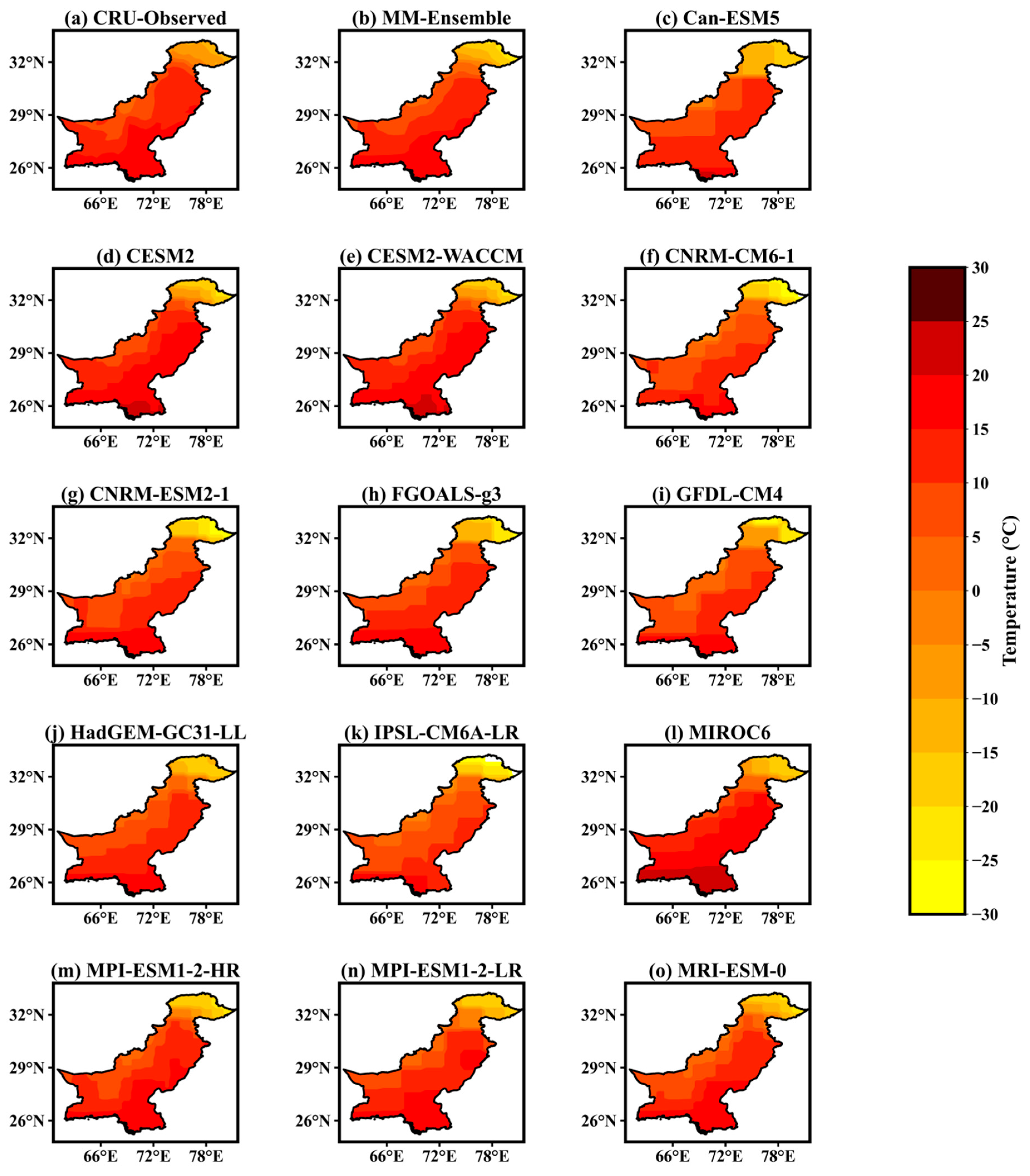
3.3. Winter Mean Temperature Climatology

Winter (DJF) mean temperature climatology for CRU, MM-Ensemble, and models is displayed in Figure 4. During DJF, CRU patterns showed a temperature of 20 °C to 25 °C over the southeast and coastal belt, 5 °C to 15 °C over central and western parts, and −10 °C to 10 °C over northern regions. MM-Ensemble, Can-ESM5, CESM2, MIROC6, MPI-ESM1-2-HR, and MRI-ESM-0 were consistent with observed patterns well in a range of −5 °C to 25 °C over southern parts. Over the north, consistent to the observed temperature patterns were simulated (in range of −20 °C to 5 °C) by MM-Ensemble, Can-ESM5, CESM2, CESM-WACCM, and MIROC6, while the remaining models largely overestimated the mean temperature following the results of [53]. Overall, MM-Ensemble, Can-ESM5, CESM2 CESM2-WACCM, and HadGEM-GC31-LL performed well (range of −5 °C to 25 °C) over the country. The DJF simulations followed a dipole structure with higher temperatures over southern parts and lower at higher and northwestern latitudes, as well as on the east-west stretch. The overall simulations for JJA and DJF temperature matched the findings of previous studies [2,27,35].

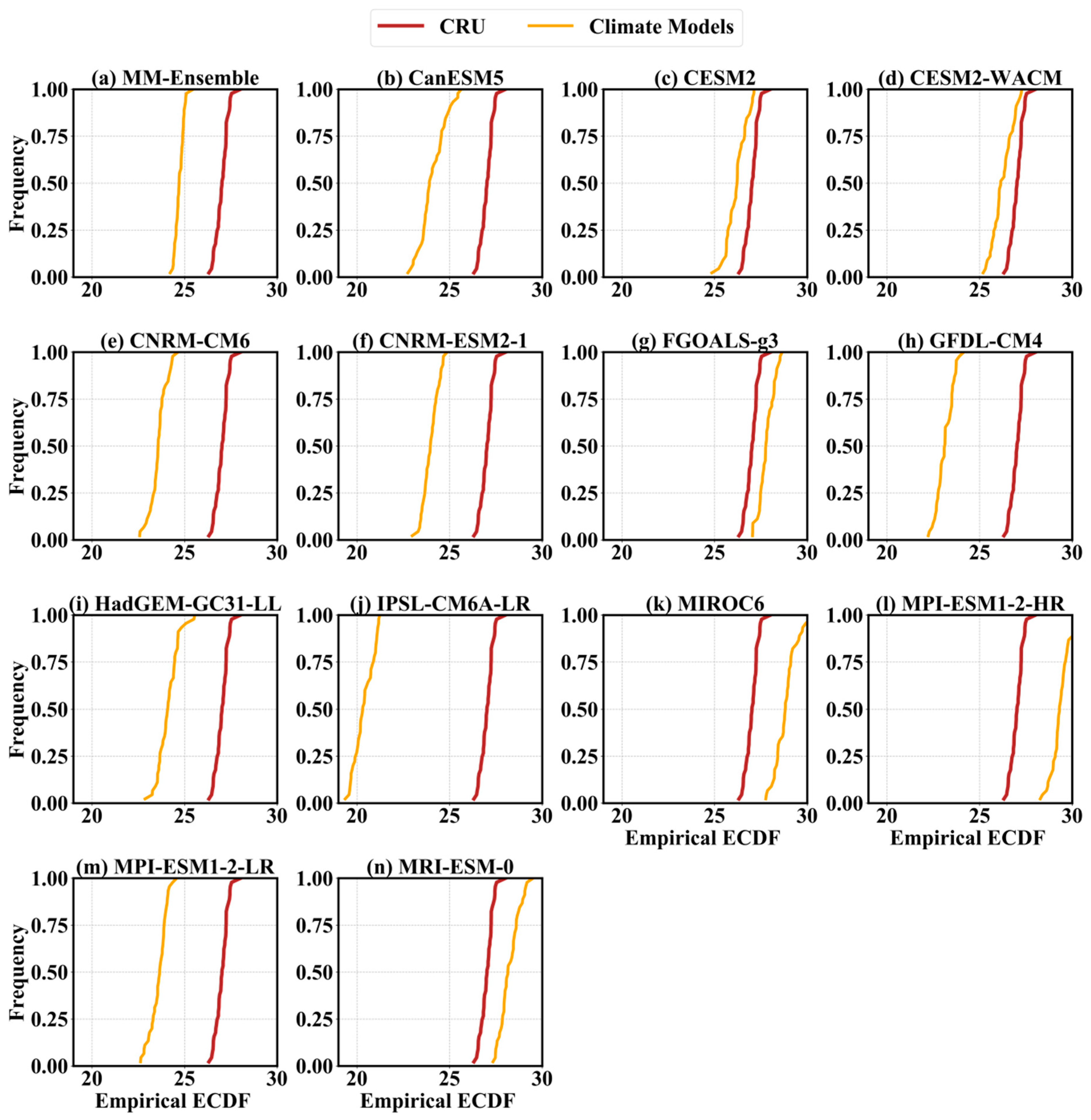
3.4. JJA Empirical Cumulative Distribution Function

The empirical cumulative distribution frequencies (ECDFs) of temperature for JJA presented in Figure 5 were utilized to get an insight into the frequency of occurrence and underestimations/ overestimations in monthly temperatures for CRU, MM-Ensemble, and models over Pakistan. The MM-Ensemble, CanESM5, CESM2, CESM2-WACCM, CNRM-CM6, CNRM-ESM2-1, GFDL-CM4, HadGEM-GC31-LL, IPSL-CM6A-LR, and MPI-ESM1-2-LR underestimated the monthly mean temperature (between 20 °C and 27 °C), complimentary to mean JJA temperature underestimates in the northwestern and central regions displayed in Figure 3. FGOALS-g3, MIROC6, MPI-ESM1-2HR, and MRI-ESM-0 overestimated the mean temperature between 26 °C and 30 °C, therefore complemented to Figure 3. CESM2, CESM2-WACCM, FGOALS-g3, and MRI-ESM-0 complemented CRU temperature distribution between 26 °C and 28 °C. A study by Tatebe et al. [54] using the MIROC6 model observed the highest warm bias and RMSE for surface temperature across Asia and the Middle East for MIROC6 compared to those of MIROC5. It was attributed to underestimating mid-level cloud cover, downward OSR (sum of net shortwave and net longwave radiation), and aerosol–radiation interaction. Such bias also usually occurs in many climate models.
Overestimations and underestimations identified biases in models, the presence of systematic inherent errors that developed under unrealistic response to forcings, or unpredictable internal variability different from observations. Other errors included errors of convective parameterizations and unresolved sub-grid scale orography. Many errors were solvable through bias correction techniques; however, biases due to nonlinearity and complex dynamical processes were uncorrectable at the current model developments [55].

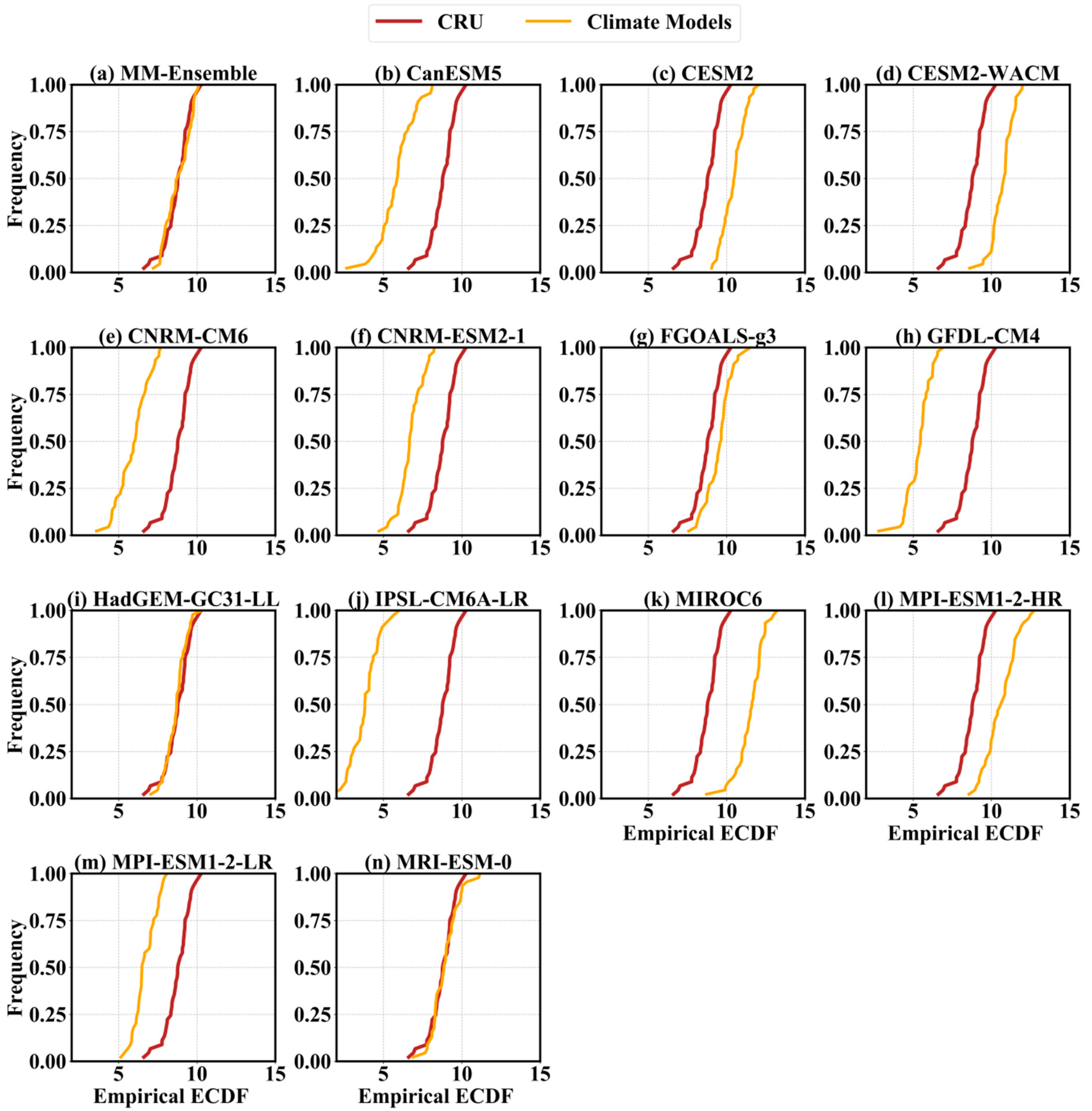
3.5. Winter Empirical Cumulative Distribution Function

The winter (DJF) ECDF for 1970–2014 over Pakistan is shown in Figure 6. The MM-Ensemble, FGOALS-g3, HadGEM-GC31-LL, MPI-ESM1-2-HR, and MRI-ESM-0 displayed similarly to the observed temperature distribution of 7 °C to 10 °C with small over/underestimations in models. CanESM5, CNRM-CM6, CNRM-ESM2-1, GFDL-CM4, IPSL-CM6A-LR, and MPI-ESM1-2-LR underestimated temperature distribution between 3 °C and 10 °C. While CESM2, CESM2-WACCM, FGOALS-g3, MIROC6, and MPI-ESM1-2-HR overestimated temperature between 9 °C and 12.5 °C, conforming to Figure 4. Many models exhibited lower over/underestimation ranges in DJF compared to those in JJA, identifying less bias in simulations. Further bias and RMSE analysis will give a clear picture of bias spread across models.

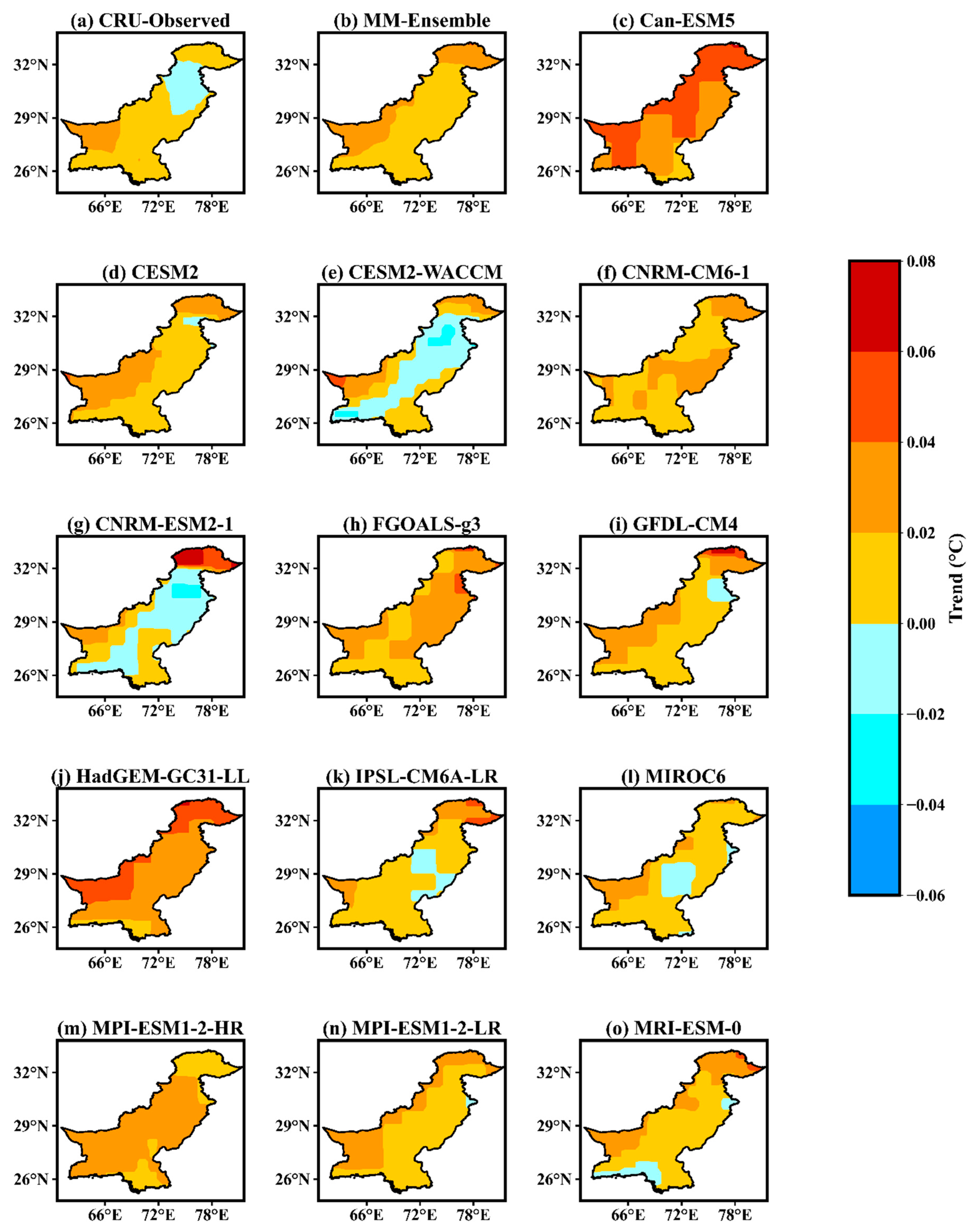
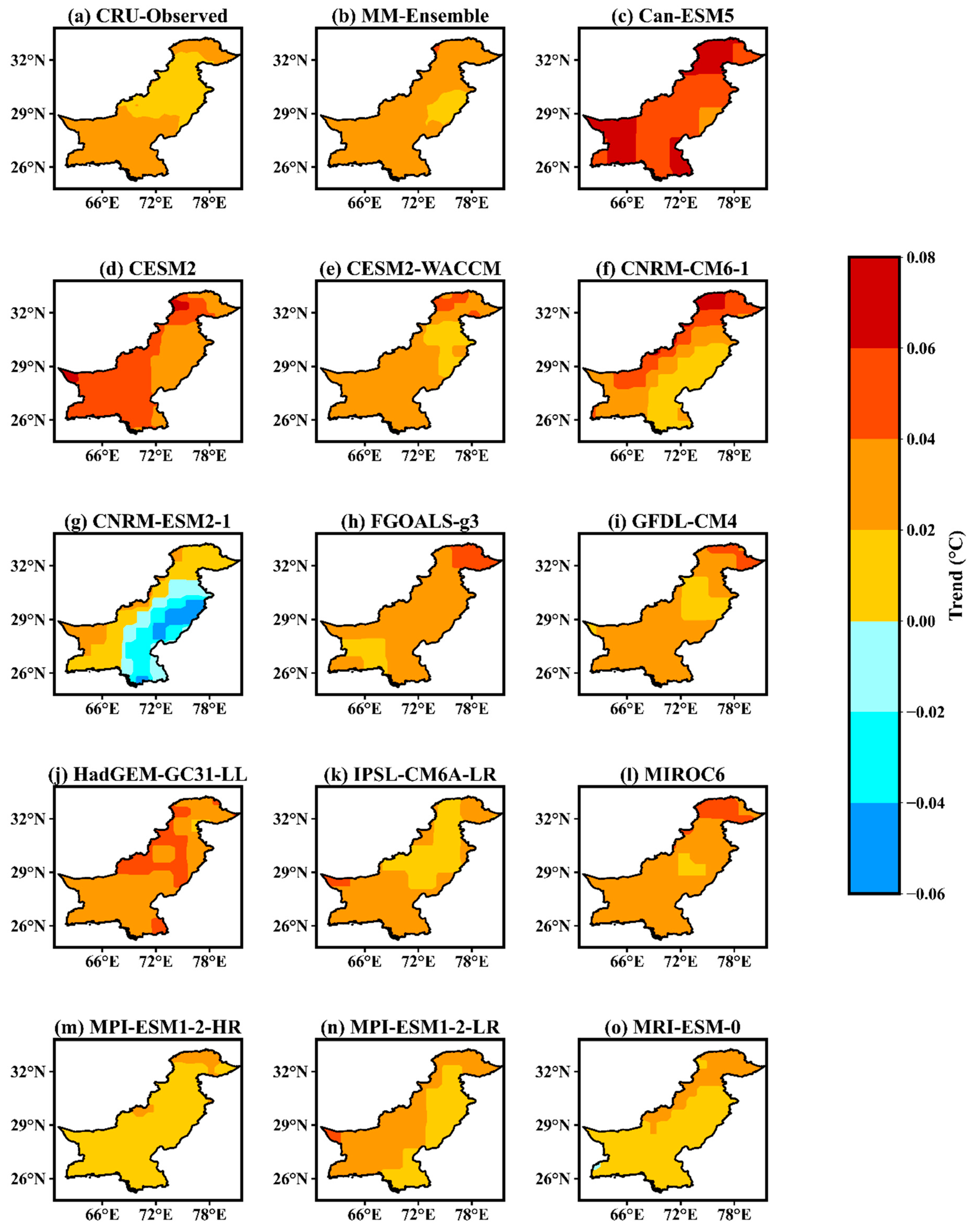
3.6. Summer and Winter Spatiotemporal Trend Analysis

The summer (JJA) and winter (DJF) spatiotemporal trend change (Table 2, Figure 7 and Figure 8) distribution for CRU, MM-Ensemble, and models for 1970–2104 over Pakistan were detected using the Mann–Kendall trend test and Sen’s slope estimator. Sen’s slope estimator gave the trend slope in time series, while the MK test gave the magnitude of trend strength. During JJA, CRU exhibited an increasing mean temperature trend of 0.016 °C/year, while MM-Ensemble showed a significant increasing trend of 0.022 °C/year. All models except for MIROC6 (0.009 °C/year) showed a significant increase in temperature trends for JJA. FGOALS-g3 and CanESM5 exhibited the highest trends in the season. The CESM2-WACCM, CNRM-ESM2-1 and MPI-ESM1-2-LR showed trends (0.019 °C, 0.017 °C, 0.019 °C/year) similar to CRU/observed trends. Historical studies with CMIP5 models [35,53,56] observed similar increasing trends in the summer season over Pakistan. Winter (DJF) mean surface temperature trends exhibited a significant increase in CRU (0.023 °C/year) and most models. Only CNRM-ESM2-1, IPSL-CM6A-LR, MPI-ESM1-2-HR, and MRI-ESM-0 revealed insignificant increasing trends. Most proximate trends to CRU were shown by IPSL-CM6A-LR (0.020 °C/year) and MPI-ESM1-2-LR (0.020 °C/year) models; the highest significant trend is shown by MM-Ensemble (0.070 °C/year). Other studies [35,53] also approved an increase in DJF surface mean temperature over Pakistan with higher warming rates than in JJA season, dominantly over the northern regions. These results were sufficiently in agreement with the spatial JJA and DJF climatology (Figure 3 and Figure 4) and trends (Figure 7 and Figure 8) in this study.
The JJA spatial trend change distribution for models, ensemble, and observed datasets over Pakistan is displayed in Figure 7. The results indicated a warming pattern of temperature over most of Pakistan (0.01 °C –0.06 °C/year), except for models such as CESM2-WACCM, CNRM-ESM2-1, and MIROC6 and CRU display, which showed negative trends over some northern and southern regions. CanESM and HadGEM-GC31-LL displayed the highest warming rate of 0.01 °C to 0.08 °C/year over the entire country, with the highest shown over northern and northwestern regions. Overall, MME-Ensemble, CanESM5, CESM2, CNRM_CM6-1, FGOALS-g3, HadGEM-GC31-LL, and MRI-ESM-0 indicated the highest warming rates over north and northwest areas, in the range of 0.01 to 0.08 °C/year.
Figure 8 shows the DJF spatial distribution of mean temperature trend change from models, ensemble, and CRU over Pakistan. The datasets showed a clear warming trend over the whole country, especially over the northern, western, and southwestern regions in the range of 0.02 °C–0.06 °C/year, while some central-eastern parts showed lower warming rates (0.01 °C–0.04 °C/year). However, CNRM-ESM2-1 showed negative trends over central-eastern to southeastern regions (−0.01 °C to −0.06 °C/year). Overall, most models such as Can-ESM5, CESM2, CESM2, CNRM-CM6-1, FGOALS-g3, HadGEM-GC31-LL, and MIROC6 showed higher (0.02 °C–0.08 °C/year) warming rates over northern and northwestern mountainous regions than in the other areas. Additionally, a higher warming rate in DJF compared to that of JJA over Pakistan and north regions was visible in the outputs. The present trend results were similar to study results by [27,33,34,35], where warming trends were found across the country, with higher warming over northern regions.
The higher warming rates at higher altitudes were attributed to the increase in the magnitude of snow-albedo feedback mechanism, an increase in incoming thermal radiation, and surface heat loss [16,34]. The other factors aiding in higher warming rates across Pakistan could be associated to surface-based feedbacks, increase in thermal radiation budget, aerosol (CFCs and hydrocarbon-based) concentrations, increasing urbanization rates, increasing industrialization, population growth, and intensive land-use change practices [8,9].

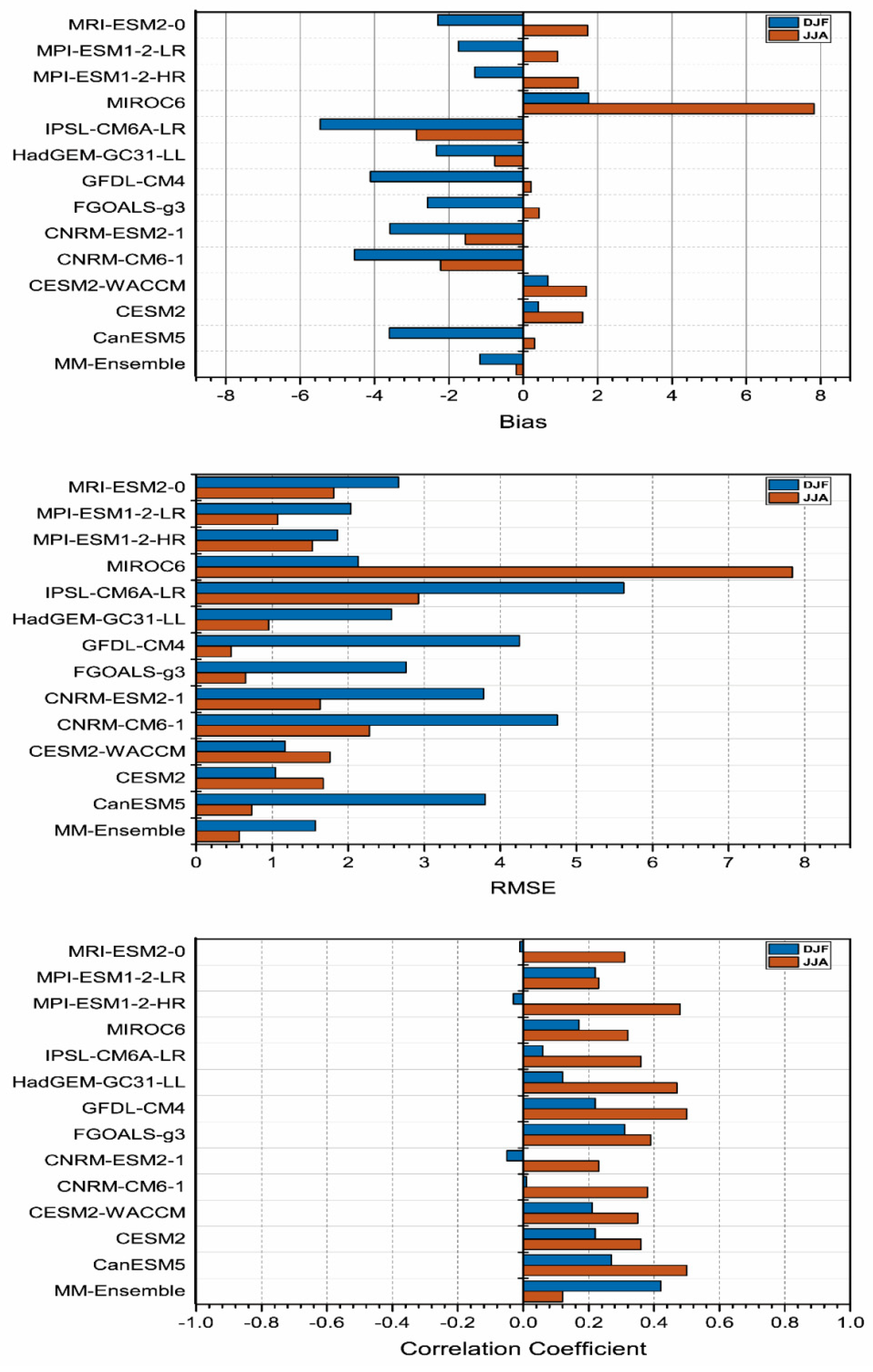
3.7. Temporal Bias, Correlation, and RMSE

A model with low bias and RMSE with higher correlation coefficient (CC) magnitudes is usually presumed as a well-performing and accounted for projecting future climate characteristics. This study employed three important statistical metrics to measure model performance capability to capture JJA and DJF CRU/observed mean temperature patterns over Pakistan for 1970–2014 and is shown in Figure 9. These metrics were calculated as area-averaged over the whole of Pakistan on JJA and DJF seasonal mean datasets. The long-term bias for JJA and DJF presented in Figure 9 (top) shows diverse results.
During JJA, four models and MM-Ensemble displayed cold/negative bias, with IPSL-CM6A-LR exhibiting the highest (−3 °C) bias while the MM-Ensemble showed the lowest of −0.2 °C. MM-Ensemble, CanESM5, FGOALS-g3, and GFDLCM4 performed well overall, with the lowest warm and cold bias of −1.3 °C to 0.2 °C; although MIROC6 showed the highest warm (poor performance) bias of 7.8 °C. The higher warm biases in MIROC6 have been observed in many parts of the world, especially in the Middle East and Mediterranean regions [54]. During DJF, most models exhibit negative/cold bias signaling underestimations within the range of <−6 °C, with the highest value of −5.7 °C by IPSL-CM6A-LR; MM-Ensemble showed the lowest warm bias (−1.3 °C). MM-Ensemble, CESM2, CESM2-WACCM, MPI-ESM1-2-HR performed well overall, with the lowest cold and warm bias in the range of 0.1 °C to −1.6 °C for DJF. The results indicate an increase in winter temperatures in the study period. Model biases and other uncertainties resulted from differences in aspects of model parameterizations, (coarse) resolution, and (poor) representation of atmospheric physics and chemistry processes [57].
The RMSE for JJA and DJF (Figure 9, middle) showed comparatively lower values during JJA in a range of <3 °C; except MIROC6 had a very high value (7.9 °C). MM-Ensemble, CanESM5, GFD-LCM4, FGOALS, and HadGEM-GC31-LL yielded the lowest RMSE in the range of 0.3 °C to 0.9 °C, justifying their better performance. For DJF, most models (except CESM2, CESM2-WACCM) exhibited comparatively higher values of RMSE against the observed dataset in the range of 1 °C to >4 °C. MM-Ensemble, CESM2, CESM2-WACCM, and MPI-ESM1-2-HR contributed the lowest values in the range of 1.0 °C to 1.9 °C, showing satisfactory performance for temperature simulation.
The JJA and DJF correlation coefficient (Figure 9, lower) for MM-Ensemble and model simulations with observed mean temperature defined their ability to capture the observed patterns. Most models in JJA showed positive CC values in the range of 0.2–0.5, performing better in replicating observed mean temperature values. CanESM5, GFDL-CM4, HadGEM-GC31-LL, and MPI-ESM1-2-HR displayed the highest CC values in the range of 0.42–0.51. Model ensembles reduced the models’ spread, although it may often have smoothed internal climate natural variability, resulting in different simulations than in observed patterns [28]. In DJF, most models, except CNRM-ESM2-1, MPI-ESM1-2-HR, and MRI-ESM2-0, exhibited a positive CC in the range of 0.01–0.2, showing weak similarity to observations. MM-Ensemble, CanESM5, and FGOALS yielded the highest CC values in the range of 0.25–0.41. Overall, in JJA and DJF, most models performed reasonably in simulating the observed mean temperature. The weak correlations between models and the observations were not a constraint in climate analysis applications since they may not have precisely depicted a specific weather event in a particular year; instead, they showed the aggregate of such events [48].

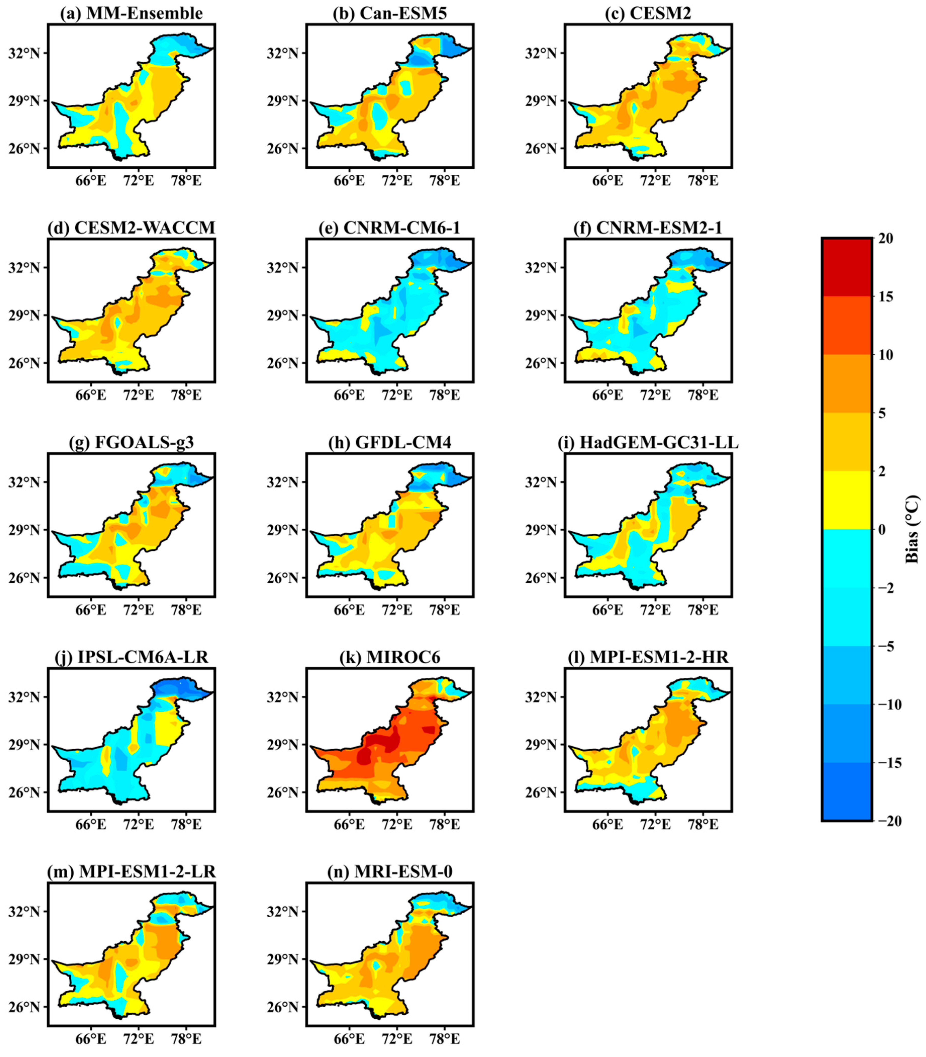
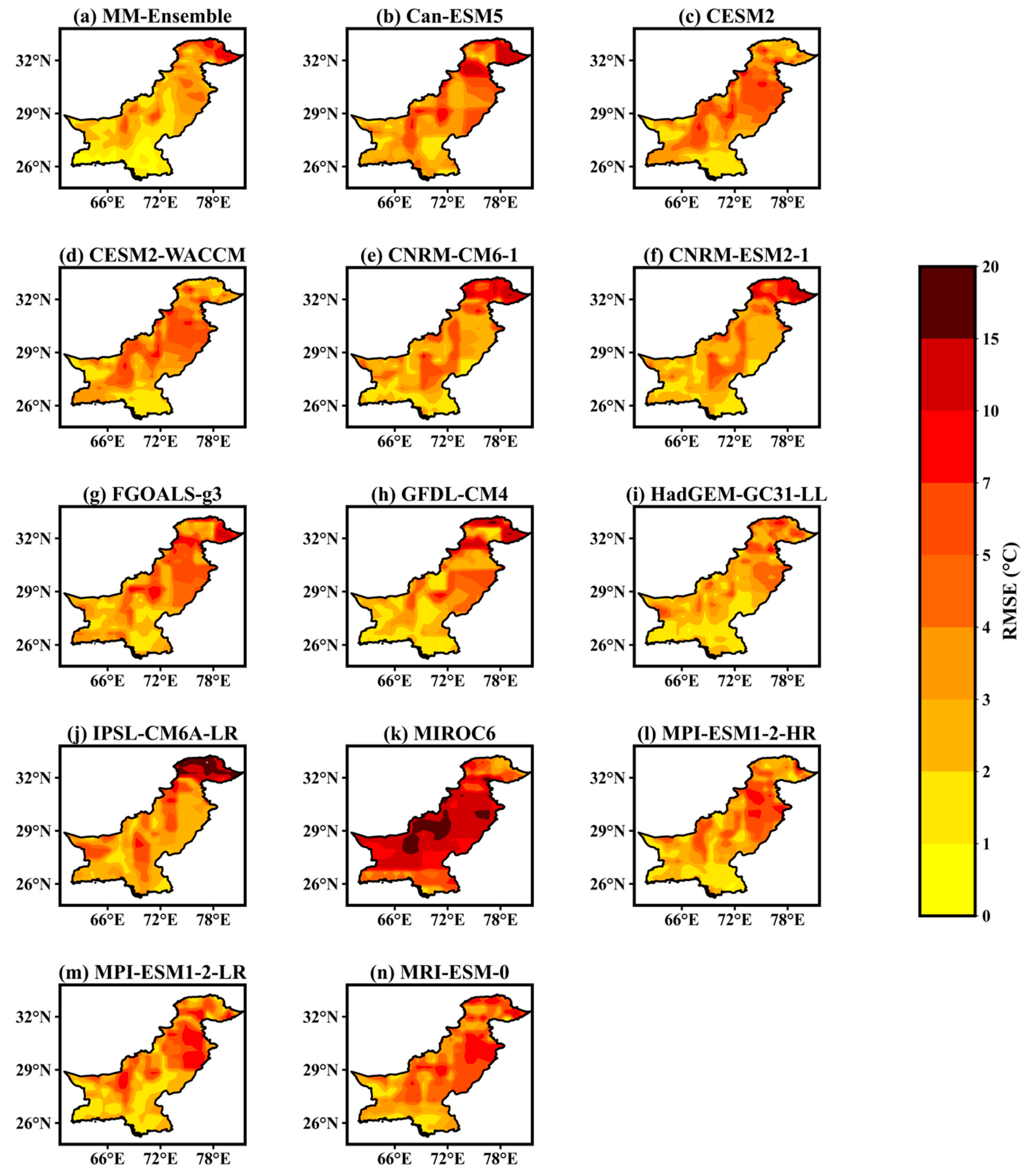
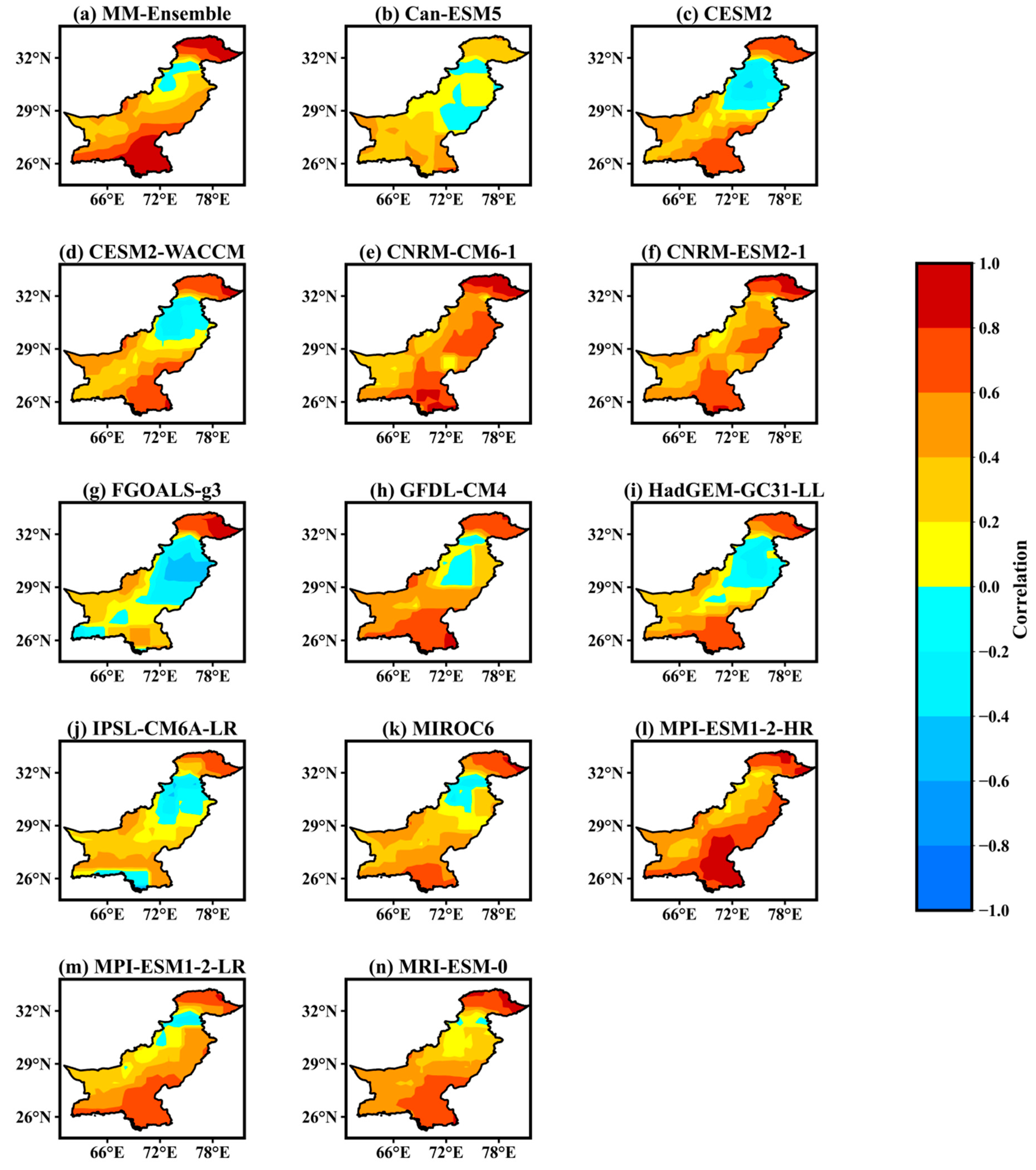
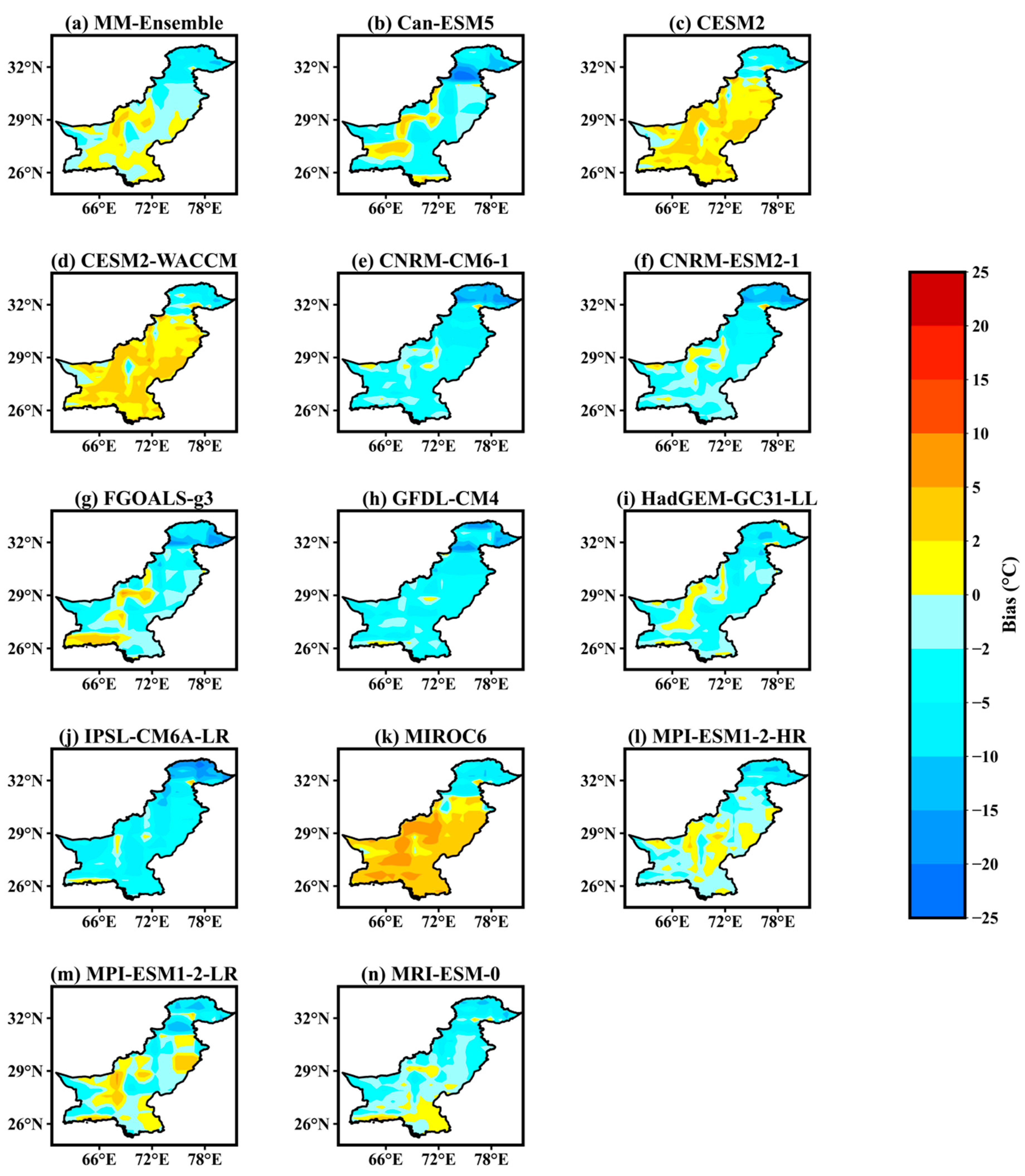
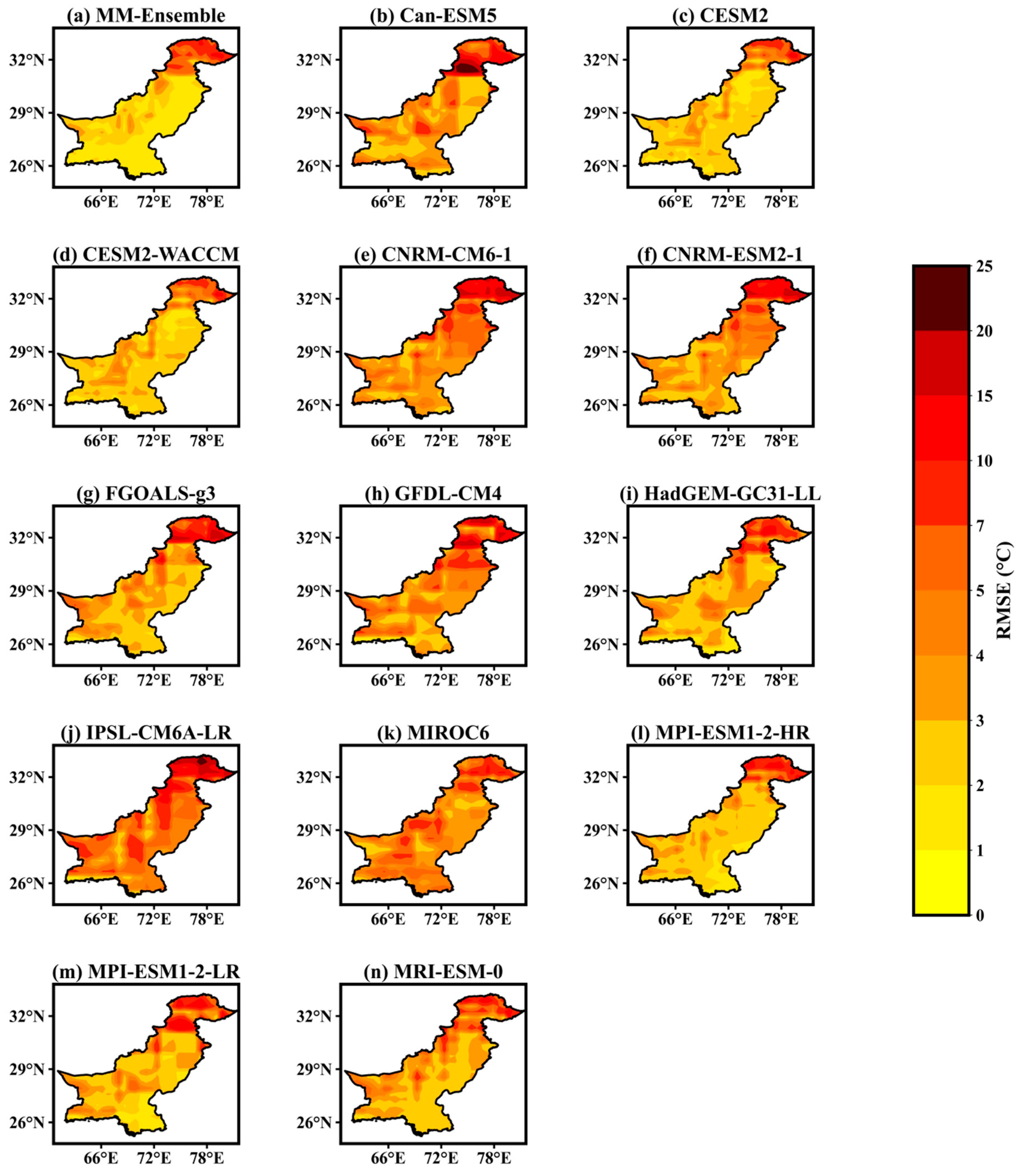
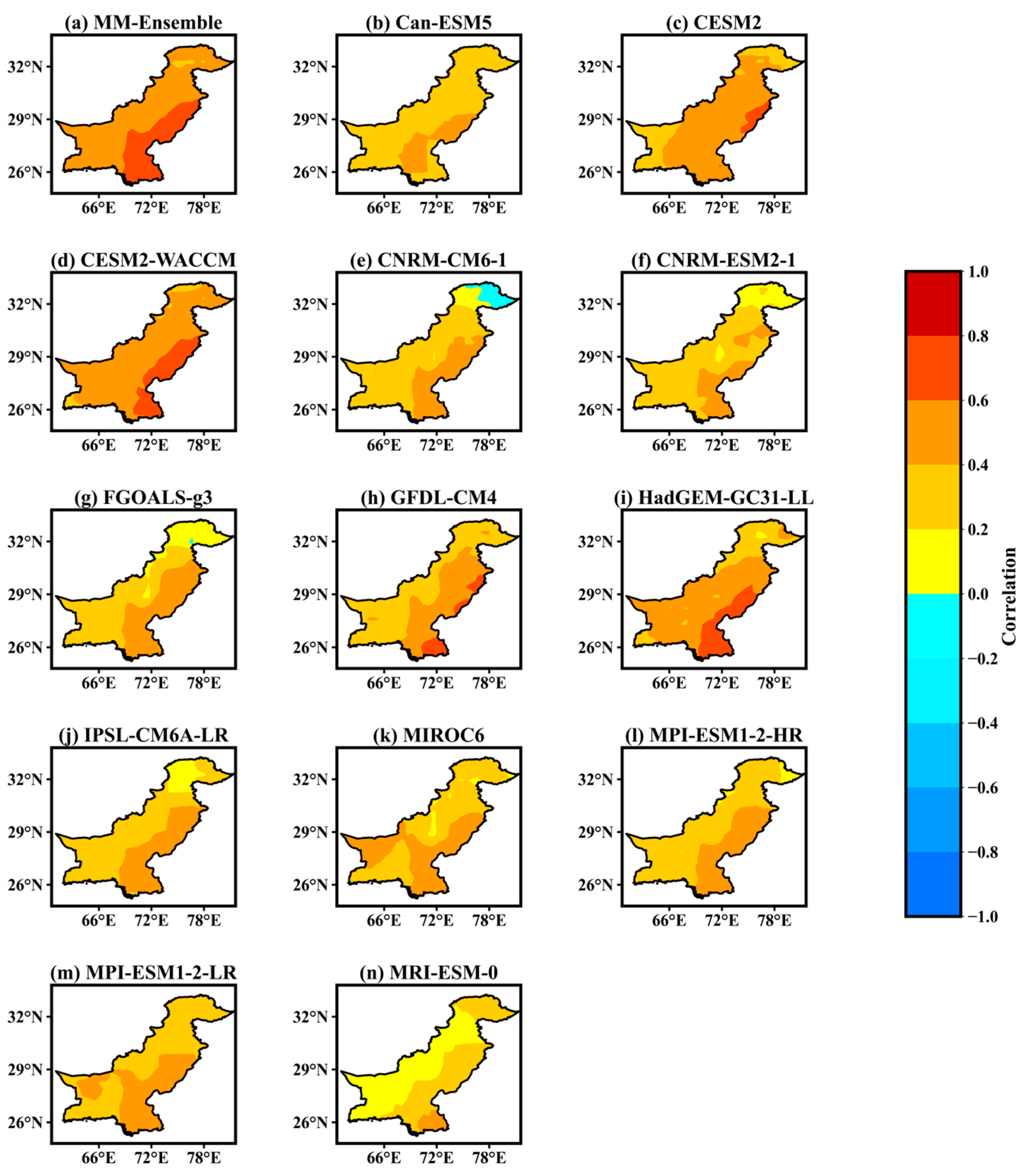
3.8. Summer Bias, RMSE, and Correlation Coefficient

Eyeball verification of spatial statistical metrics of bias, RMSE, and correlation coefficient (CC) was utilized for JJA, as plotted in Figure 10, Figure 11 and Figure 12. The JJA spatial bias (Figure 10) displayed varying warm and cold bias, identifying underestimation/overestimation of mean temperature by models. The MM-Ensemble, CanESM5, CESM2-WACCM, CNRM-CM6, CNRM-ESM2-1, FGOALS-g3, GFDL-CM4, and IPSL-CM6A-LR underestimated temperature (−8 °C to −20 °C range) over the extreme north, while CNRM-CM6, CNRM-ESM2-1, and IPSL-CM6A-LR underestimated (−1°C to −10 °C) over southern regions. The MM-Ensemble, CESM2, CESM-WACCM, FGOALS, MPI-ESM1-2-HR, and MPI-ESM1-2-LR exhibited the lowest bias in the range of −10 °C to 10 °C. MIROC6 displayed the highest warm biases, and IPSL-CM6A-LR showed the coldest biases among all models. Persistent warm biases in CMIP5 GCMs simulations over southern plains and cold biases over the mountainous regions of north and northwest areas of Pakistan were also revealed by [56]. The above results also coincided with the temporal bias (Figure 9) distribution for models and ensemble over Pakistan.
The JJA RMSE (difference in values of CRU observations and model simulations) of mean temperature is shown in Figure 11. Ideally, a near-zero RMSE value indicates close matching outputs of observed climate features. MM-Ensemble, CNRM-ESM2, HadGEM-GC31-LL, MPI-ESM1-2-HR exhibited the lowest RMSE (0.1 °C to 10 °C range) for most parts of the country, particularly over southern, southeastern, and southwestern regions. However, IPSL-CM6A-LR, MIROC6, and MRI-ESM-0 exhibited the highest (underperformed) RMSE (7 °C to 10 °C) over few northern and northeastern parts, presumably for the models’ passiveness to resolve inherent issues of mountainous topography resolution, cloud cover, and snow-albedo feedback parameterization as observed by [18,58].
MM-Ensemble and models’ CC values for JJA mean temperatures plotted in Figure 12 show their skill to capture CRU temperature variability patterns. Can-ESM5, CESM2, CESM2-WACCM, FGOALS-g3, GFDL-CM4, HadGEM-GC31-LL, IPSL-CM6A-LR, and MIROC6 showed low to negative CC (0.2 to −0.4) over central east to central west regions, depicting weak agreement for models and observed temperature. Strong agreement (>0.7) was exhibited by all models (except Can-ESM) over northern areas. Most models also captured (>0.5) the observed temperature well over southeast and coastal regions, except for FGOALS-g3 and IPSL-CM6A-LR. Overall, MM-Ensemble, CNRM-CM6-1, CNRM-ESM2-1, MPI-ESM1-2-HR, and MRI-ESM-0 exhibited the highest CC (−0.2 to >0.8) for most parts of the country.

3.9. Winter Spatial Bias, RMSE, and Correlation Coefficient Metrics

The winter (DJF) season spatial bias, RMSE, and correlation are given in Figure 13, Figure 14 and Figure 15. The DJF bias (Figure 13) displayed a mix of warm (overestimations) and cold (underestimations) bias by the models. MM-Ensemble, Can-ESM5, CNRM-CM6-1, CNRM-ESM2-1, FGOALS-g3, GFDL-CM4, HadGEM-GC31-LL, IPSL-CM6A-LR, MPI-ESM1-2-HR, MPI-ESM1-2-LR, and MRI-ESM-0 identified (−0.1 °C to −25 °C) cold bias over northern, central-eastern, and a few southern parts. MM-Ensemble, CESM2, CESM2-WACCM, and MIROC6 exhibited a warm bias/overestimation (0.1 °C to 10 °C) range over northern to southern regions. MM-Ensemble, CESM2, CESM2-WACCM, CNRM-CM6-1, HadGEM-GC31-LL, and MRI-ESM-0 yielded the lowest bias in the −0.1 °C to 10 °C range, conforming to their better performance in simulating the observed DJF mean temperature. A study by [32] found matching results for bias during JJA (mostly cold bias in the range of −2 °C to >−10 °C) across the whole of Pakistan and in DJF, with mostly warm bias >2 °Cover few northern and southern regions. Similarly, [53] revealed high cold bias over the country’s northern parts at annual and seasonal scales.
The DJF season RMSE (Figure 14) analysis exhibited a higher RMSE (>5 °C) over northern and the northwestern parts by all models and ensemble. While the MM-Ensemble, CESM2, CESM2-WACCM, and MPI-ESM1-2-HR exhibited the lowest RMSE (0.1 °C to >15 °C) in the country, especially over southern regions. The remaining models gave higher values (>5 °C) over most areas, specifically over northern areas.
The correlation coefficient (CC) for the DJF season (Figure 15) revealed the strongest CC (0.01 to <0.8) by MM-Ensemble, CESM2, CESM2-WACCM, GFDL-CM4, and HadGEM-GC31-LL for the whole country, dominantly across the central-eastern to south-eastern regions. The CNRM-CM6-1 showed an apparent disagreement with CRU data over the extreme north; MRI-ESM-0 and CNRM-ESM2-1 agreed (weak) with CRU over the whole country. Overall, the majority of models displayed a weak positive CC over the country.

4. Discussion

In this study, CMIP6 models simulated seasonal mean temperature reasonably over Pakistan.
Earlier, Ather et al. [32] found higher temperatures over southern Pakistan from two GFDL CMIP5 (CM2p1, CM3.0) model runs during DJF (cold westerlies in north and north-westerlies) and southern areas in JJA for (heat low/land-sea heat gradient and role of moisture flux) in recent years.
In an attribution study, Bollasina et al. [59] detected the role of thermal forcing and low-level northerlies (indirect) over the Hindu Kush Mountains in deepening heat low during JJA and DJF over the north. Babar et al. [35] utilized CMIP5 models and established the BCC-CSM1.1, HadGEM2-CC, and NorESM1-M models as best performing with higher temperatures over southern parts compared to northern parts (cold bias). For the CMIP5 ensemble, a recent work by Das et al. [60] exhibited higher JJA temperatures over north, central, southwest, and southeast parts of Pakistan forced by anthropogenic activities and industrialization. Meanwhile, Ahmed et al. [2] observed lower temperature extremes over northern regions and higher over southern regions from CMIP5 multi-mode-ensemble, NorESM1-M, MIROC5, BCC-CSM1-1, and ACCESS1-3 simulations close to CRU patterns. Besides the mentioned local climate factors, model resolution (influence of physical and biological processes representation), benchmark datasets quality (consequence magnitude and the direction of comprehensive circulation processes), model climate sensitivity (planetary energy balance, CO2 change-led earth warming), and changes in the spatiotemporal extent of forcings (annual and seasonal variations) determine simulation accuracy [52,57,61]. The models’ simulated seasonal variability over South Asia could be due to the embedded convection schemes’ dynamic behavior over the sub-regions [62]. The CRU datasets go through extensive quality control measures and gauge station numbers to reduce uncertainties in climate variability patterns [46]. The multi-decadal temperature changes may be forced by anthropogenic and natural forcing (volcanic aerosol forcing) or could arise unforced from the climate system due to climate sensitivity and unforced variability [63].
Further, in the study, CMIP6 models and CRU datasets showed a significant increase in mean temperature trends in this study, particularly higher over the north during DJF over Pakistan. Many studies [12,13,14,64] identified increasing trends in winter and summer (0.17 °C–0.37 °C/decade) over Pakistan’s central and northern regions. Babar et al. [35] discovered a higher (0.21 °C/decade) winter mean temperature rise than in summer (0.21 °C/decade) for CRU; 0.11°C–0.06 °C/decade in UDEL dataset and 0.10°C–0.09 °C/decade in CMIP5 ensemble. The CanESM, CCSM, IPSL, and MPI models showed higher trends for winter, and summer over northern and southwestern regions had the highest trends (0.6 °C/decade) for all datasets. Supportively, [34] identified higher warming rates over the northern, southeastern, and southwestern regions. The global temperature warming has amplified at high altitude environments due to elevation-dependent warming through changes in the response of mechanisms like snow albedo, surface-based feedbacks, water vapor changes, latent heat release, surface water vapor, radiative flux changes, surface heat loss, temperature change, and aerosols, and earth’s energy balance system [65]. Over the Tibetan Plateau, the snow-albedo feedback has been identified as the primary factor for higher warming and ice melting [66,67]. Moreover, Archer et al. [68] observed a high positive correlation between summer runoff (snowmelt water) and temperature increase over the Upper Indus Basin of Pakistan. Further, Fatima et al. [69] concluded that with the rapid melting of Hindu Kush–Karakorum–Himalayan glaciers, floods and glacial lake outburst floods (GLOFs) are obvious, and depletion of freshwater availability is the next phase. Southern Pakistan also experiences warming temperatures under the influence of industrialization and transportation boom, land-use change, population pressure, vegetation loss, water resources absence, and pollution (aerosols and other chemical compounds), which pave the way for heatwaves and droughts [8,9,70].
The role of internal variability (variability of climate system occurring in absence of external forcings like atmospheric, oceanic, and coupled ocean-atmosphere processes systems) as a major driver of climate change uncertainty is manifested in calculations of trends and climatology estimates [71,72]. Historical trends are highly influenced by internal variability and are useful for climatology information analysis under multi-realizations of larger ensemble members, and vice versa to the forced variability trends. Historical multi-run members’ trends are highly influenced by internal variability and forced variability is dominant in future projection trend patterns across model runs. In addition, across most model run pairs (in multi-run member cases), changes are small, and less than intermodal differences, the evaluation of models’ spatial climatology can be more informative. The single run-based analyzed trends by any chance may resemble or not resemble observations, possibly bringing ambiguity (considering noise fitting as trends) to model evaluation [72]. Deser et al. [73] studied that near-term (like 2010–2030) surface temperature responses need large multiple realizations ensemble members at middle and higher latitudes to acquire robust estimates of forced and internal variability of climate system in models. Moreover, climate change monitoring can be best served by focusing on thermodynamic components (e.g., air temperature, inbound radiations, ocean heat content) of the climate system. Any historical model-based trend study should involve multiple realizations for models involved, although such realizations possess less effects on future climate projections.
Most models and ensembles in the study performed well in simulating observed patterns of temperature in JJA, although with some differences. Improved performance of CMIP6 models across JJA can be attributed to improvements in climate forcings’ effects, aerosols’ representation and resolution, detailed parameterization of cloud cover, vegetation, surface convection, physiographic features, diurnal cycles of models, and inclusion of the earth system models [27,31,74]. A CMIP5 study [53] yielded MIROC5, CESM1-WACCM, GISS-E2-H-CC, GISS-E2-H, and MRI-CGCM3 models’ better performance in JJA (than DJF) with less bias and RMSE, and sound correlation with CRU. Whilst [35] found INM-CM, IPSL, BCC, EC-Earth, NorESM, and GISS performing well for JJA and DJF mean temperature simulation, model-ensemble displayed a higher cold bias in summer and winter.
The differences in simulations to observed patterns could be due to the complex and diverse geography, landscape, and climatology of Pakistan; ranging from mountains in the north and plains, deserts, and coasts in the south with a blend of humid, arid, semi-arid, and coastal to hyper-arid climates [2,34,75]. Simulation variances also emerge from systematic errors due to internal variability and different responses to forcings, creating contradictory atmospheric processes [24]. Models performed passively across diverse topography and geography for their sensitivity/passiveness to variations such as mountains, with resolution issues all functioning simultaneously [76]. Moreover, higher climate sensitivity caused overestimations and underestimations, leading to biases in present and future climate estimates [29].

5. Conclusions

Current and historical simulations for climate variables are vital to understanding the prevailing climate and future climate scenarios. This study employed the mean temperature variable from the CMIP6 models for the summer (June–July–August) and winter (December–January–February) seasons for 1970–2014 over Pakistan. Thirteen CMIP6 utilized JJA and DJF climatology, ECDF, trend, bias, RMSE, and correlation coefficient (CC). The highest mean temperature for 1970–2014 over Pakistan was observed (24 to 35 °C) during JJA months and the minimum during DJF months (2 to 9 °C).
The JJA and DJF spatial mean climatology by CRU, models, and MM-Ensemble displayed a dipole structure over north-south with low to high temperature scales. The ECDF for JJA temperature was identified close to the observed and smaller temperature distribution range than the DJF season.
Further, DJF spatiotemporal trends revealed higher increasing trends for all datasets across Pakistan, especially over northern regions, than in JJA, although few models showed insignificant trends.
A model of low bias and RMSE with a higher correlation coefficient (CC) is considered as a well-performing in simulating specific climate characteristics. The temporal bias, RMSE, and CC in JJA and DJF yielded diverse outcomes. For JJA, most models yielded low bias (2 °C to −2 °C), low RMSE (<1.9 °C) and higher CC (0.01–0.4) values for 1970–2014 simulations. However, in DJF, higher negative bias (0.21 °C to −3 °C), higher RMSE (<4 °C), and lower CC values (0.01–0.30) were detected for the 1970–2014 period.
The JJA spatial bias, RMSE, and CC metrics analysis discovered a higher warm bias (1 °C to 20 °C), low RMSE (1 °C to 15 °C), and high CC values (0.2 to >0.8) over the whole of Pakistan. A strong cold bias (0 °C to −20 °C), higher RMSE (2 °C–25 °C range), and a positive but weak CC (0.2–0.8) was detected for the majority of models and ensemble in DJF. The cold bias/underestimation also signaled towards the higher observed temperature during DJF for 1970–2014.
This study revealed diverse outputs of models’ simulations and their performance in two critical seasons over Pakistan. After assessing models for bias, RMSE, and CC performance metrics, CanESM5, CESM2, CESM2-WACCM, GFDL-CM4, HadGEM-GC31-LL, MPI-ESM1-2-HR, MPI-ESM1-2-HR, and MRI-ESM-0 were found to perform better overall in simulating observed temperatures over Pakistan. These models could be utilized in future temperature projection and impact studies over Pakistan.

Author Contributions

Conceptualization, R.K. and B.A.; methodology, R.K. and B.A.; software, H.B.; validation, R.K., H.B., and B.A.; formal analysis, R.K., B.A., and G.T.; investigation, G.T. and B.A.; resources, G.T.; data curation, B.A.; writing—original draft preparation, R.K. and B.A.; writing—review and editing, R.K., G.T., B.A., F.L. and H.B.; visualization, R.K., H.B. and F.L.; supervision, G.T.; project administration, G.T. and B.A.; funding acquisition, G.T. All authors have read and agreed to the published version of the manuscript.

Funding

The National Key Research and Development Program of China (2017YFA0603804) and National Natural Science Foundation of China (41575070) supported this work.

Acknowledgments

The authors acknowledge Nanjing University of Information Science and Technology (NUIST) for providing a favorable environment and infrastructural needs for conducting research. Special appreciation to the World Climate Research Programme (WCRP) for availing data to use for evaluation studies. The lead author is grateful to NUIST for granting him a scholarship to pursue Ph.D. studies. The authors acknowledge the help of NUIST-High Performance Computing (HPC) Cluster in providing data computation facilities for this study.

Conflicts of Interest

In a unanimous agreement, all authors declare no conflict of interest in the present study.

References

  1. IPCC. Synthesis Report. Contribution of Working Groups I, II and III to the Fifth Assessment Report of the Intergovernmental Panel on Climate Change; Core Writing Team, Pachauri, R.K., Meyer, L.A., Eds.; IPCC: Geneva, Switzerland, 2014; p. 151. [CrossRef] [Green Version]
  2. Ahmed, K.; Sachindra, D.A.; Shahid, S.; Demirel, M.C.; Chung, E.-S. Selection of multi-model ensemble of general circulation models for the simulation of precipitation and maximum and minimum temperature based on spatial assessment metrics. Hydrol. Earth Syst. Sci. 2019, 23, 4803–4824. [Google Scholar] [CrossRef] [Green Version]
  3. Perkins-Kirkpatrick, S.E.; Gibson, P.B. Changes in regional heatwave characteristics as a function of increasing global temperature. Sci. Rep. 2017, 7, 1256. [Google Scholar] [CrossRef] [PubMed]
  4. IPCC. Contribution of Working Group I to the Fifth Assessment Report of the Intergovernmental Panel on Climate Change; Stocker, T.F., Qin, D., Plattner, G.K., Tignor, M., Allen, S.K., Boschung, J., Nauels, A., Xia, Y., Bex, V., Midgley, P.M., Eds.; Cambridge University Press: Cambridge, UK, 2013.
  5. Sivakumar, M.V.K.; Stefanski, R. Climate Change in South Asia, in Climate Change and Food Security in South Asia; Springer: Dordrecht, The Netherlands, 2010; pp. 13–30. [Google Scholar]
  6. Wester, P.; Mishra, A.; Mukherji, A.; Shrestha, A.B. The Hindu Kush Himalaya Assessment; Springer International Publishing: Cham, Switzerland, 2019. [Google Scholar]
  7. Kreft, S.; Eckstein, D.; Melchior, I. Global Climate Risk Index 2017: Who Suffers Most from Extreme Weather Events? Germanwatch e.V.: Bonn, Germany, 2017; ISBN 9783943704495. [Google Scholar]
  8. Haider, S.; Adnan, S. Classification and Assessment of Aridity Over Pakistan Provinces (1960–2009). Int. J. Environ. 2014, 3, 24–35. [Google Scholar] [CrossRef] [Green Version]
  9. Rasul, G.; Afzal, M.; Zahid, M.; Ali Bukhari, S.A. Climate Change in Pakistan Focused on Sindh Province. In Pakistan Meteorological Department Technical Report; No. PMD-25/2012; Pakistan Meteorological Department: Islamabad, Pakistan, 2012; p. 55. [Google Scholar]
  10. Afzaal, M.; Haroon, M.A. Interdecadal Oscillations and the Warming Trend in the Area-Weighted Annual Mean Temperature of Pakistan. Pak. J. Meteorol. 2009, 6, 13–19. [Google Scholar]
  11. McSweeney, C.; New, M.; Lizcano, G. Climate Change Country Profiles Documentation. National Communication Support Program. 2008; pp. 1–26. Available online: https://www.geog.ox.ac.uk/research/climate/projects/undp-cp/UNDP_reports/Pakistan/Pakistan.hires.report.pdf (accessed on 20 September 2020).
  12. Khan, N.; Shahid, S.; bin Ismail, T.; Wang, X.J. Spatial distribution of unidirectional trends in temperature and temperature extremes in Pakistan. Theor. Appl. Climatol. 2019, 136, 899–913. [Google Scholar] [CrossRef]
  13. Ullah, S.; You, Q.; Ali, A.; Ullah, W.; Jan, M.A.; Zhang, Y.; Xie, W.; Xie, X. Observed changes in maximum and minimum temperatures over China-Pakistan economic corridor during 1980–2016. Atmos. Res. 2019, 216, 37–51. [Google Scholar] [CrossRef]
  14. Adnan, S.; Ullah, K.; Gao, S.; Khosa, A.H.; Wang, Z. Shifting of agro-climatic zones, their drought vulnerability, and precipitation and temperature trends in Pakistan. Int. J. Climatol. 2017, 37, 529–543. [Google Scholar] [CrossRef]
  15. Balling, R.C.; Kiany, M.S.K.; Roy, S.S. Anthropogenic signals in Iranian extreme temperature indices. Atmos. Res. 2016, 169, 96–101. [Google Scholar] [CrossRef]
  16. Rasul, G.; Dahe, Q.; Chaudhry, Q.Z. Global Warmin and Melting Glaciers along Southern Slopes of HKH Ranges. Pak. J. Meteorol. 2008, 5, 63–76. [Google Scholar]
  17. Roy, S.S.; Keikhosravi Kiany, M.S.; Balling, R.C. A Significant Population Signal in Iranian Temperature Records. Int. J. Atmos. Sci. 2016, 2016, 1–7. [Google Scholar] [CrossRef] [Green Version]
  18. Nie, S.; Fu, S.; Cao, W.; Jia, X. Comparison of monthly air and land surface temperature extremes simulated using CMIP5 and CMIP6 versions of the Beijing Climate Center climate model. Theor. Appl. Climatol. 2020, 140, 487–502. [Google Scholar] [CrossRef]
  19. Abbas, F.; Rehman, I.; Adrees, M.; Ibrahim, M.; Saleem, F.; Ali, S.; Rizwan, M.; Salik, M.R. Prevailing trends of climatic extremes across Indus-Delta of Sindh-Pakistan. Theor. Appl. Climatol. 2018, 131, 1101–1117. [Google Scholar] [CrossRef]
  20. Del Río, S.; Anjum Iqbal, M.; Cano-Ortiz, A.; Herrero, L.; Hassan, A.; Penas, A. Recent mean temperature trends in Pakistan and links with teleconnection patterns. Int. J. Climatol. 2013, 33, 277–290. [Google Scholar] [CrossRef]
  21. Fang, S.; Qi, Y.; Yu, W.; Liang, H.; Han, G.; Li, Q.; Shen, S.; Zhou, G.; Shi, G. Change in temperature extremes and its correlation with mean temperature in mainland China from 1960 to 2015. Int. J. Climatol. 2017, 37, 3910–3918. [Google Scholar] [CrossRef]
  22. Ahmadalipour, A.; Rana, A.; Moradkhani, H.; Sharma, A. Multi-criteria evaluation of CMIP5 GCMs for climate change impact analysis. Theor. Appl. Climatol. 2017, 128, 71–87. [Google Scholar] [CrossRef] [Green Version]
  23. Ramesh, K.V.; Goswami, P. Assessing reliability of regional climate projections: The case of Indian monsoon. Sci. Rep. 2014, 4. [Google Scholar] [CrossRef] [PubMed]
  24. Eyring, V.; Bony, S.; Meehl, G.A.; Senior, C.A.; Stevens, B.; Stouffer, R.J.; Taylor, K.E. Overview of the Coupled Model Intercomparison Project Phase 6 (CMIP6) experimental design and organization. Geosci. Model Dev. 2016, 9, 1937–1958. [Google Scholar] [CrossRef] [Green Version]
  25. Hausfather, Z.; Peters, G.P. Emissions—The ‘business as usual’ story is misleading. Nature 2020, 577, 618–620. [Google Scholar] [CrossRef]
  26. Grose, M.R.; Narsey, S.; Delage, F.P.; Dowdy, A.J.; Bador, M.; Boschat, G.; Chung, C.; Kajtar, J.B.; Rauniyar, S.; Freund, M.B.; et al. Insights From CMIP6 for Australia’s Future Climate. Earth’s Future 2020, 8. [Google Scholar] [CrossRef] [Green Version]
  27. Almazroui, M.; Saeed, S.; Islam, M.; Ismail, M. Projections of Precipitation and Temperature over the South Asian Countries in CMIP6. Earth Syst. Environ. 2020, 4, 297–320. [Google Scholar] [CrossRef]
  28. Zhao, T.; Chen, L.; Ma, Z. Simulation of historical and projected climate change in arid and semiarid areas by CMIP5 models. Chin. Sci. Bull. 2014, 59, 412–429. [Google Scholar] [CrossRef]
  29. Tokarska, K.B.; Stolpe, M.B.; Sippel, S.; Fischer, E.M.; Smith, C.J.; Lehner, F.; Knutti, R. Past warming trend constrains future warming in CMIP6 models. Sci. Adv. 2020, 6. [Google Scholar] [CrossRef] [PubMed] [Green Version]
  30. National Research Council. Understanding Earth’s Deep Past: Lessons for Our Climate Future; National Academies Press: Washington, DC, USA, 2011; p. 20. [Google Scholar]
  31. O’Neill, B.C.; Tebaldi, C.; Van Vuuren, D.P.; Eyring, V.; Friedlingstein, P.; Hurtt, G.; Knutti, R.; Kriegler, E.; Lamarque, J.F.; Lowe, J.; et al. The Scenario Model Intercomparison Project (ScenarioMIP) for CMIP6. Geosci. Model Dev. 2016, 9, 3461–3482. [Google Scholar] [CrossRef] [Green Version]
  32. Athar, U.A.H.; Latif, A.N.M. An AOGCM based assessment of interseasonal variability in Pakistan. Clim. Dyn. 2018, 50, 349–373. [Google Scholar] [CrossRef]
  33. Ali, S.; Eum, H.-I.; Jaepil, C.; Li, D.; Khan, F.; Dairaku, K.; Shrestha, M.L.; Hwang, S.; Naseem, W.; Khan, I.A.; et al. Assessment of climate extremes in future projections downscaled by multiple statistical downscaling methods over Pakistan. Atmos. Res. 2019, 222, 114–133. [Google Scholar] [CrossRef]
  34. Sajjad, H.; Ghaffar, A. Observed, simulated and projected extreme climate indices over Pakistan in changing climate. Theor. Appl. Climatol. 2018, 137, 255–281. [Google Scholar] [CrossRef]
  35. Babar, Z.A.; Zhi, X.; Ge, F.; Riaz, M.; Mahmood, A.; Sultan, S.; Shad, M.A.; Aslam, C.M.; Ahmad, M.F. Assessment of Southwest Asia Surface Temperature Changes: CMIP5 20th and 21st Century Simulations. Pak. J. Meteorol. 2016, 13, 1–15. [Google Scholar]
  36. Lelieveld, J.; Proestos, Y.; Hadjinicolaou, P.; Tanarhte, M.; Tyrlis, E.; Zittis, G. Strongly increasing heat extremes in the Middle East and North Africa (MENA) in the 21st century. Clim. Chang. 2016, 137, 245–260. [Google Scholar] [CrossRef] [Green Version]
  37. Knutti, R.; Sedláček, J. Robustness and uncertainties in the new CMIP5 climate model projections. Nat. Clim. Chang. 2013, 3, 369–373. [Google Scholar] [CrossRef]
  38. Zhang, B.; Soden, B.J. Constraining Climate Model Projections of Regional Precipitation Change. Geophys. Res. Lett. 2019, 46, 10522–10531. [Google Scholar] [CrossRef]
  39. Sarfaraz, S. The Sub-Regional Classification of Pakistan’s Winter Precipitation Based on Principal Components Analysis. Pak. J. Meteorol. 2014, 10, 57–66. [Google Scholar]
  40. Iqbal, Z.; Shahid, S.; Ahmed, K.; Ismail, T.; Nawaz, N. Spatial distribution of the trends in precipitation and precipitation extremes in the sub-Himalayan region of Pakistan. Theor. Appl. Climatol. 2019, 137, 2755–2769. [Google Scholar] [CrossRef]
  41. Farooqi, A.B.; Khan, A.H.; Mir, H. Climate Change Perspective in Pakistan. Pak. J. Meteorol. 2005, 2, 11–21. [Google Scholar]
  42. Ikram, F.; Afzaal, M.; Bukhari, S.A.A.; Ahmed, B. Past and Future Trends in Frequency of Heavy Rainfall Events over Pakistan. Pak. J. Meteorol. 2016, 12, 57–78. [Google Scholar]
  43. Vermeulen, J.L.; Hillebrand, A.; Geraerts, R. A comparative study of k-nearest neighbour techniques in crowd simulation. Comput. Animat. Virtual Worlds 2017, 28. [Google Scholar] [CrossRef]
  44. Mallika, M.; Sundaram, S.M.; Nirmala, M. Annual mean temperature prediction of India using K-Nearest Neighbour technique. Appl. Math. Sci. 2015, 9, 613–616. [Google Scholar] [CrossRef]
  45. Pincus, R.; Batstone, C.P.; Patrick Hofmann, R.J.; Taylor, K.E.; Glecker, P.J. Evaluating the present-day simulation of clouds, precipitation, and radiation in climate models. J. Geophys. Res. Atmos. 2008, 113, D14209. [Google Scholar] [CrossRef]
  46. Harris, I.; Jones, P.D.; Osborn, T.J.; Lister, D.H. Updated high-resolution grids of monthly climatic observations—The CRU TS3.10 Dataset. Int. J. Climatol. 2014, 34, 623–642. [Google Scholar] [CrossRef] [Green Version]
  47. Ongoma, V.; Chen, H.; Gao, C. Evaluation of CMIP5 twentieth century rainfall simulation over the equatorial East Africa. Theor. Appl. Climatol. 2019, 135, 893–910. [Google Scholar] [CrossRef]
  48. Ayugi, B.; Tan, G.; Gnitou, G.T.; Ojara, M.; Ongoma, V. Historical evaluations and simulations of precipitation over East Africa from Rossby centre regional climate model. Atmos. Res. 2020, 232. [Google Scholar] [CrossRef]
  49. Mann, H.B. Nonparametric Tests against Trend. Econometrica 1945, 13, 245. [Google Scholar] [CrossRef]
  50. Kendall, M.G. Rank Correlation Methods, 4th ed.; Griffin: London, UK, 1975; p. 202. [Google Scholar]
  51. Ayugi, B.O.; Tan, G.; Ongoma, V.; Mafuru, K.B. Circulations Associated with Variations in Boreal Spring Rainfall over Kenya. Earth Syst. Environ. 2018, 2, 421–434. [Google Scholar] [CrossRef]
  52. You, Q.; Min, J.; Kang, S. Rapid warming in the tibetan plateau from observations and CMIP5 models in recent decades. Int. J. Climatol. 2016, 36, 2660–2670. [Google Scholar] [CrossRef]
  53. Nadia Rehman, M.A.; Ali, S. Assessment of CMIP5 climate models over South Asia and climate change projections over Pakistan under representative concentration pathways. Int. J. Glob. Warm. 2018, 16, 381. [Google Scholar] [CrossRef]
  54. Tatebe, H.; Ogura, T.; Nitta, T.; Komuro, Y.; Ogochi, K.; Takemura, T.; Sudo, K.; Sekiguchi, M.; Abe, M.; Saito, F.; et al. Description and basic evaluation of simulated mean state, internal variability, and climate sensitivity in MIROC6. Geosci. Model Dev. Discuss. 2018, 1–92. [Google Scholar] [CrossRef] [Green Version]
  55. Cannon, A.J.; Sobie, S.R.; Murdock, T.Q. Bias correction of GCM precipitation by quantile mapping: How well do methods preserve changes in quantiles and extremes? J. Clim. 2015, 28, 6938–6959. [Google Scholar] [CrossRef]
  56. Iqbal, W.; Zahid, M. Historical and Future Trends of Summer Mean Air Temperature over South Asia. Pak. J. Meteorol. 2014, 10, 67–74. [Google Scholar]
  57. Gusain, A.; Ghosh, S.; Karmakar, S. Added value of CMIP6 over CMIP5 models in simulating Indian summer monsoon rainfall. Atmos. Res. 2020, 232, 104680. [Google Scholar] [CrossRef]
  58. Sillmann, J.; Kharin, V.V.; Zhang, X.; Zwiers, F.W.; Bronaugh, D. Bronaugh. Climate extremes indices in the CMIP5 multimodel ensemble: Part 1. Model evaluation in the present climate. J. Geophys. Res. Atmos. 2013, 118, 1716–1733. [Google Scholar] [CrossRef]
  59. Bollasina, M.; Nigam, S. The summertime ‘heat’ low over Pakistan/northwestern India: Evolution and origin. Clim. Dyn. 2011, 37, 957–970. [Google Scholar] [CrossRef] [Green Version]
  60. Das, L.; Akhter, J.; Dutta, M.; Meher, J.K. Ensemble-based CMIP5 simulations of monsoon rainfall and temperature changes over South Asia. Chall. Agro-Environ. Res. Monsoon Asia 2015, 6, 41–60. [Google Scholar] [CrossRef]
  61. Eyring, V.; Cox, P.M.; Flato, G.M.; Gleckler, P.J.; Abramowitz, G.; Caldwell, P.; Collins, W.D.; Gier, B.K.; Hall, A.D.; Hoffman, F.M.; et al. Taking climate model evaluation to the next level. Nat. Clim. Chang. 2019, 9, 102–110. [Google Scholar] [CrossRef] [Green Version]
  62. Hassan, M.; Du, P. Regional climate model simulation for temperature and precipitation over South Asia using different physical parameterisation schemes. Int. J. Glob. Warm. 2018, 14, 1–20. [Google Scholar] [CrossRef]
  63. Neukom, R.; Barboza, L.A.; Erb, M.P.; Shi, F.; Emile-Geay, J.; Evans, M.N.; Franke, J.; Kaufman, D.S.; Lücke, L.; Rehfeld, K.; et al. Consistent multidecadal variability in global temperature reconstructions and simulations over the Common Era. Nat. Geosci. 2019, 12, 643–649. [Google Scholar] [CrossRef] [Green Version]
  64. Nawaz, Z.; Li, X.; Chen, Y.; Guo, Y.; Wang, X.; Nawaz, N. Temporal and spatial characteristics of precipitation and temperature in Punjab, Pakistan. Water 2019, 11, 1916. [Google Scholar] [CrossRef] [Green Version]
  65. Pepin, N.; Bradley, R.S.; Diaz, H.F.; Baraër, M.; Caceres, E.B.; Forsythe, N.; Fowler, H.; Greenwood, G.; Hashmi, M.Z.; Liu, X.D.; et al. Elevation-dependent warming in mountain regions of the world. Nat. Clim. Chang. 2015, 5, 424–430. [Google Scholar] [CrossRef] [Green Version]
  66. Yan, L.; Liu, X. Has Climatic Warming over the Tibetan Plateau Paused or Continued in Recent Years ? J. Earth Ocean Atmos. Sci. 2014, 1, 13–28. [Google Scholar]
  67. Rangwala, I.; Miller, J.R.; Russell, G.L.; Xu, M. Using a global climate model to evaluate the influences of water vapor, snow cover and atmospheric aerosol on warming in the Tibetan Plateau during the twenty-first century. Clim. Dyn. 2010, 34, 859–872. [Google Scholar] [CrossRef]
  68. Archer, D.R.; Fowler, H.J. Conflicting signals of climatic change in the upper Indus Basin. J. Clim. 2006, 19, 4276–4293. [Google Scholar] [CrossRef] [Green Version]
  69. Fatima, E.; Hassan, M.; Hasson, S.U.; Ahmad, B.; Ali, S.S.F. Future water availability from the western Karakoram under representative concentration pathways as simulated by CORDEX South Asia. Theor. Appl. Climatol. 2020, 1–16. [Google Scholar] [CrossRef]
  70. Ullah, S.; You, Q.; Ullah, W.; Hagan, D.F.T.; Ali, A.; Ali, G.; Zhang, Y.; Jan, M.A.; Bhatti, A.S.; Xie, W. Daytime and nighttime heat wave characteristics based on multiple indices over the China–Pakistan economic corridor. Clim. Dyn. 2019, 53, 6329–6349. [Google Scholar] [CrossRef]
  71. Perkins-Kirkpatrick, S.E.; Fischer, E.M.; Angélil, O.; Gibson, P.B. The influence of internal climate variability on heatwave frequency trends. Environ. Res. Lett. 2017, 12, 044005. [Google Scholar] [CrossRef]
  72. Gibson, P.B.; Perkins-Kirkpatrick, S.E.; Alexander, L.V.; Fischer, E.M. Comparing Australian heat waves in the CMIP5 models through cluster analysis. J. Geophys. Res. 2017, 122, 3266–3281. [Google Scholar] [CrossRef]
  73. Deser, C.; Phillips, A.; Bourdette, V.; Teng, H. Uncertainty in climate change projections: The role of internal variability. Clim. Dyn. 2012, 38, 527–546. [Google Scholar] [CrossRef] [Green Version]
  74. Gidden, M.; Riahi, K.; Smith, S.; Fujimori, S.; Luderer, G.; Kriegler, E.; van Vuuren, D.P.; van den Berg, M.; Feng, L.; Klein, D.; et al. Global emissions pathways under different socioeconomic scenarios for use in CMIP6: A dataset of harmonized emissions trajectories through the end of the century. Geosci. Model Dev. 2019, 12, 1443–1475. [Google Scholar] [CrossRef] [Green Version]
  75. Ahmed, K.; Shahid, S.; Wang, X.; Nawaz, N.; Khan, N. Spatiotemporal changes in aridity of Pakistan during 1901–2016. Hydrol. Earth Syst. Sci. 2019, 23, 3081–3096. [Google Scholar] [CrossRef] [Green Version]
  76. Fu, C.; Jiang, Z.; Guan, Z.; He, J.; Xu, Z.F. (Eds.) Regional Climate Studies of China; Springer Science & Business Media: Berlin/Heidelberg, Germany, 2008. [Google Scholar] [CrossRef]
Figure 1. Map of the study area (61–78° E and 23–37.5° N) showing elevation (m) in color ranges and boundary extent for proposed historical observed and simulated mean temperature in the study to be utilized.
Atmosphere 11 01005 g001
Figure 2. The annual cycle of mean temperature over Pakistan for 1970–214 based on observed climatic research unit (CRU), CMIP6 individual models, and the ensemble mean (MM-Ensemble) depicting overestimation and underestimation of temperature. The CRU is displayed in the black color line and MM-Ensemble in the red color line. The turquoise color bars on MM-Ensemble represent the deviation of values from the mean in each month.
Atmosphere 11 01005 g002
Figure 3. Spatial distribution of June–July–August (JJA) mean temperature (°C) over Pakistan for 1970–2014 for (a) CRU, (b) MM-Ensemble, (c) Can-ESM5, (d) CESM2, (e) CESM-WACCM, (f) CNRM-CM6-1, (g) CNRM-ESM2-1, (h) FGOALS-g3, (i) GFDL-CM4, (j) HadGEM-GC31-LL, (k) IPSL-CM6A-LR, (l) MIROC6, (m) MPI-ESM1-2-HR, (n) MPI-ESM-2-LR, and (o) MRI-ESM-0.
Atmosphere 11 01005 g003
Figure 4. Same as Figure 3 but for winter (December–January–February (DJF)) season.
Atmosphere 11 01005 g004
Figure 5. JJA months cumulative distribution frequency (°C/month) from observed (CRU) versus (a) MM-Ensemble, (b) Can-ESM5, (c) CESM2, (d) CESM-WACCM, (e) CNRM-CM6-1, (f) CNRM-ESM2-1, (g) FGOALS-g3, (h) GFDL-CM4, (i) HadGEM-GC31-LL, (j) IPSL-CM6A-LR, (k) MIROC6, (l) MPI-ESM1-2-HR, (m) MPI-ESM-2-LR, and (n) MRI-ESM-0 models. Red-colored line shows CRU observed ECDF and yellow lines show empirical cumulative distribution frequency (ECDF) for individual models under study and their ensemble. The x-axis shows temperature range (°C) and the y-axis shows its frequency f(x).
Atmosphere 11 01005 g005
Figure 6. Same as Figure 5, but for winter (DJF) season.
Atmosphere 11 01005 g006
Figure 7. Spatial distribution of JJA mean temperature trend slope (°C/year) over Pakistan for 1970–2014 for (a) CRU, (b) MM-Ensemble, (c) Can-ESM5, (d) CESM2, (e) CESM-WACCM, (f) CNRM-CM6-1, (g) CNRM-ESM2-1, (h) FGOALS-g3, (i) GFDL-CM4, (j) HadGEM-GC31-LL, (k) IPSL-CM6A-LR, (l) MIROC6, (m) MPI-ESM1-2-HR, (n) MPI-ESM-2-LR, and (o) MRI-ESM-0.
Atmosphere 11 01005 g007
Figure 8. Same as Figure 7, but for DJF season.
Atmosphere 11 01005 g008
Figure 9. Bias, RMSE, and correlation coefficient for models and MM-Ensemble based on CRU datasets in JJA and DJF seasons of 1970–2014 over Pakistan. The brown-colored legend key identifies the JJA metrics while the dark blue color identifies DJF season metrics.
Atmosphere 11 01005 g009
Figure 10. Spatial bias distribution of JJA mean temperature (°C) over Pakistan for 1970–2014 by (a) MM-Ensemble, (b) Can-ESM5, (c) CESM2, (d) CESM-WACCM, (e) CNRM-CM6-1, (f) CNRM-ESM2-1, (g) FGOALS-g3, (h) GFDL-CM4, (i) HadGEM-GC31-LL, (j) IPSL-CM6A-LR, (k) MIROC6, (l) MPI-ESM1-2-HR, (m) MPI-ESM-2-LR, and (n) MRI-ESM-0.
Atmosphere 11 01005 g010
Figure 11. Spatial RMSE distribution of JJA mean temperature (°C) over Pakistan for 1970–2014 by (a) MM-Ensemble, (b) Can-ESM5, (c) CESM2, (d) CESM-WACCM, (e) CNRM-CM6-1, (f) CNRM-ESM2-1, (g) FGOALS-g3, (h) GFDL-CM4, (i) HadGEM-GC31-LL, (j) IPSL-CM6A-LR, (k) MIROC6, (l) MPI-ESM1-2-HR, (m) MPI-ESM-2-LR, and (n) MRI-ESM-0.
Atmosphere 11 01005 g011
Figure 12. Spatial correlation coefficient distribution of JJA mean temperature (°C) over Pakistan for 1970–2014 by (a) MM-Ensemble, (b) Can-ESM5, (c) CESM2, (d) CESM-WACCM, (e) CNRM-CM6-1, (f) CNRM-ESM2-1, (g) FGOALS-g3, (h) GFDL-CM4, (i) HadGEM-GC31-LL, (j) IPSL-CM6A-LR, (k) MIROC6, (l) MPI-ESM1-2-HR, (m) MPI-ESM-2-LR, and (n) MRI-ESM-0.
Atmosphere 11 01005 g012
Figure 13. Same as Figure 10 but for winter (DJF) season bias.
Atmosphere 11 01005 g013
Figure 14. Same as Figure 11 but for winter (DJF) season RMSE.
Atmosphere 11 01005 g014
Figure 15. Same as Figure 12 but for winter (DJF) season correlation.
Atmosphere 11 01005 g015
Table 1. Description of CMIP6 models used in the study showing their origin, resolution, and release year. All models acquired r1i1p1 global attribute indices for this study.
NoModel NameInstituteResolution (lon._lat.)Release Year
1CanESM5Canadian Centre for Climate Modeling and Analysis (Canada).2.8 × 2.8°2019
2CESM2National Centre for Climate Research (USA).1.3 × 0.9°2018
3CESM2-WACCMNational Centre for Climate Research (USA).1.3 × 0.9°2018
4CNRM-CM6-1Centre National de Recherches Météorologiques (France).1.4 × 1.4°2017
5CNRM-ESM2-1Centre National de Recherches Météorologiques (France).1.4 × 1.4°2017
6FGOALS-g3University of Chinese Academy of Sciences.2 × 2.3°2017
7GFDL-CM4NOAA Geophysical Fluid Dynamics Laboratory, USA.2 × 2°2018
8HadGEM-GC31-LLMet Office Hadley Centre. 2016
9IPSL-CM6A-LRInstitut Pierre Simon Laplace, France.2.5 × 1.3°2017
10MIROC6National Institute for Environmental Studies, and Japan Agency for Marine-Earth Science and Technology (MIROC), Japan.1.4 × 1.4°2017
11MPI-ESM1-2-HRMax Planck Institute for Meteorology (Germany).0.9 × 0.9°2017
12MPI-ESM1-2-LRMax Planck Institute for Meteorology (Germany).1.9 × 1.9°2017
13MRI-ESM2-0Meteorological Research Institute (MRI) of the Japan Meteorological Agency (JMA).1.1 × 1.1°2017
Table 2. Mean values, trend magnitude, and Sen’s slope for trend change (°C/decade) values for observed, MM-Ensemble, and models’ simulated mean temperature for 1970–2014 summer (JJA) and winter (DJF) season over Pakistan.
DatasetsJJADJF
MeanChange °C/Year Change °C/Decade▲/▼MeanChange °C/YearChange °C/Decade▲/▼
CRU27.00.0160.157▲=8.770.0230.231▲=
Models
MM-Ensemble26.80.0220.220▲=7.520.0700.700▲=
CanESM527.30.0390.390▲=5.170.0580.578▲=
CESM228.60.0200.196▲=9.170.0420.420▲=
CESM2-WACCM28.70.0190.187▲=9.440.0320.322▲=
CNRM-CM6-124.80.0210.213▲=4.230.0330.333▲=
CNRM-ESM2-125.50.0170.174▲=5.190.0070.070▲≠
FGOALS-g327.40.0230.235▲=6.200.0320.321▲=
GFDL-CM427.20.0210.210▲=4.660.0280.280▲=
HadGEM-GC31-LL26.30.0360.361▲=6.430.0350.353▲=
IPSL-CM6A-LR24.10.0220.224▲=3.310.0200.199▲≠
MIROC634.80.0090.093▲≠10.530.0360.361▲=
MPI-ESM1-2-HR28.50.0230.233▲=7.460.0110.109▲≠
MPI-ESM1-2-LR27.90.0190.189▲=7.030.0200.204▲=
MRI-ESM2-028.80.0210.213▲=6.470.0120.122▲≠
Negative (▼) and positive (▲) Z-values indicate decreasing and increasing trends. The = and ≠ signs stand for significant and insignificant trends, respectively, at 95% confidence interval.

