Author Contributions
Conceptualization, J.M., A.R., C.V., S.C.P. and J.A.S.; methodology, J.M. and A.R.; software, J.M., C.V. and S.C.P.; validation, J.M., A.R., C.V., S.C.P. and J.A.S.; formal analysis, J.M. and A.R.; investigation, J.M. and A.R.; resources, J.M., A.R., C.V., S.C.P.; data curation, J.M. and A.R.; writing—original draft preparation, J.M., A.R. and J.A.S.; writing—review and editing, J.M., A.R. and J.A.S.; visualization, J.M. and A.R.; supervision, J.M. and A.R.; project administration, J.M. and A.R.; funding acquisition, A.R. All authors have read and agreed to the published version of the manuscript.
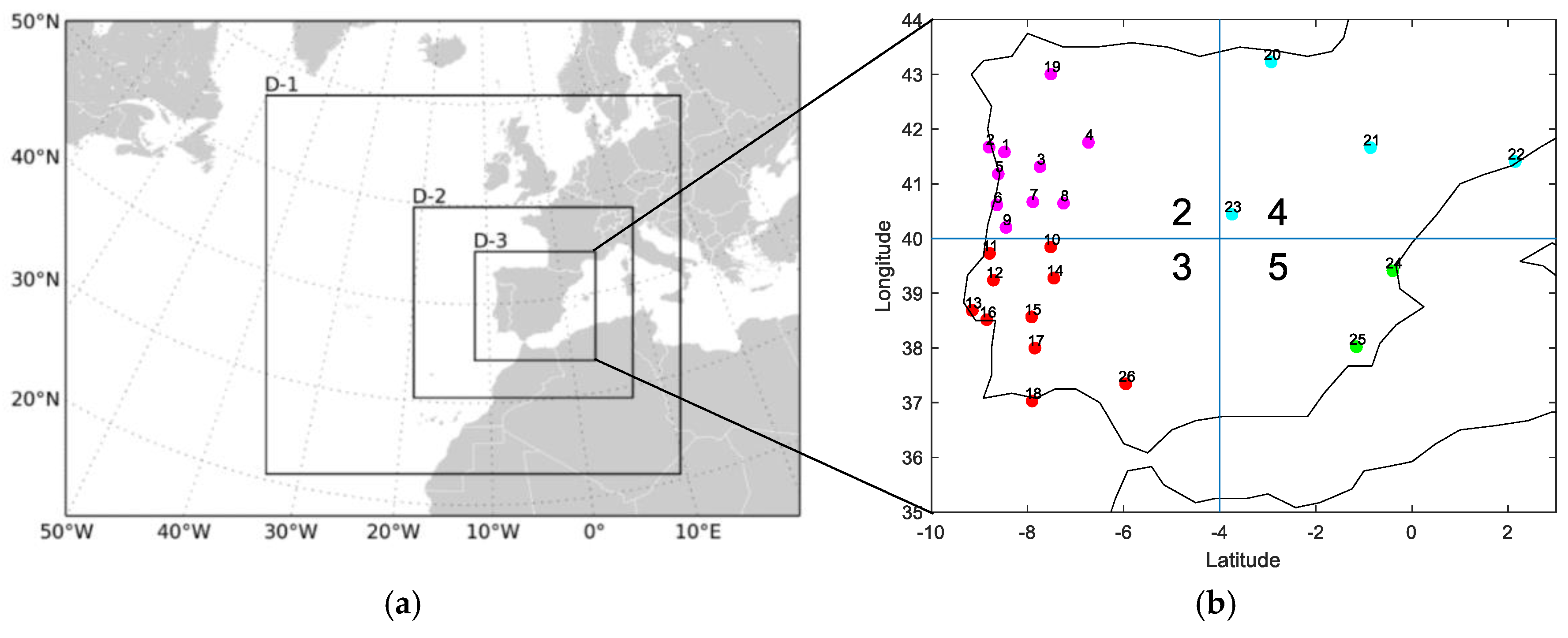
Figure 1.
(
a) The domain used in the Weather Research and Forecasting (WRF) regional implementation, with 81, 27, and 9 km of horizontal resolution [
52] and (
b) division of the studied area per regions in the Iberian Peninsula.
Figure 1.
(
a) The domain used in the Weather Research and Forecasting (WRF) regional implementation, with 81, 27, and 9 km of horizontal resolution [
52] and (
b) division of the studied area per regions in the Iberian Peninsula.
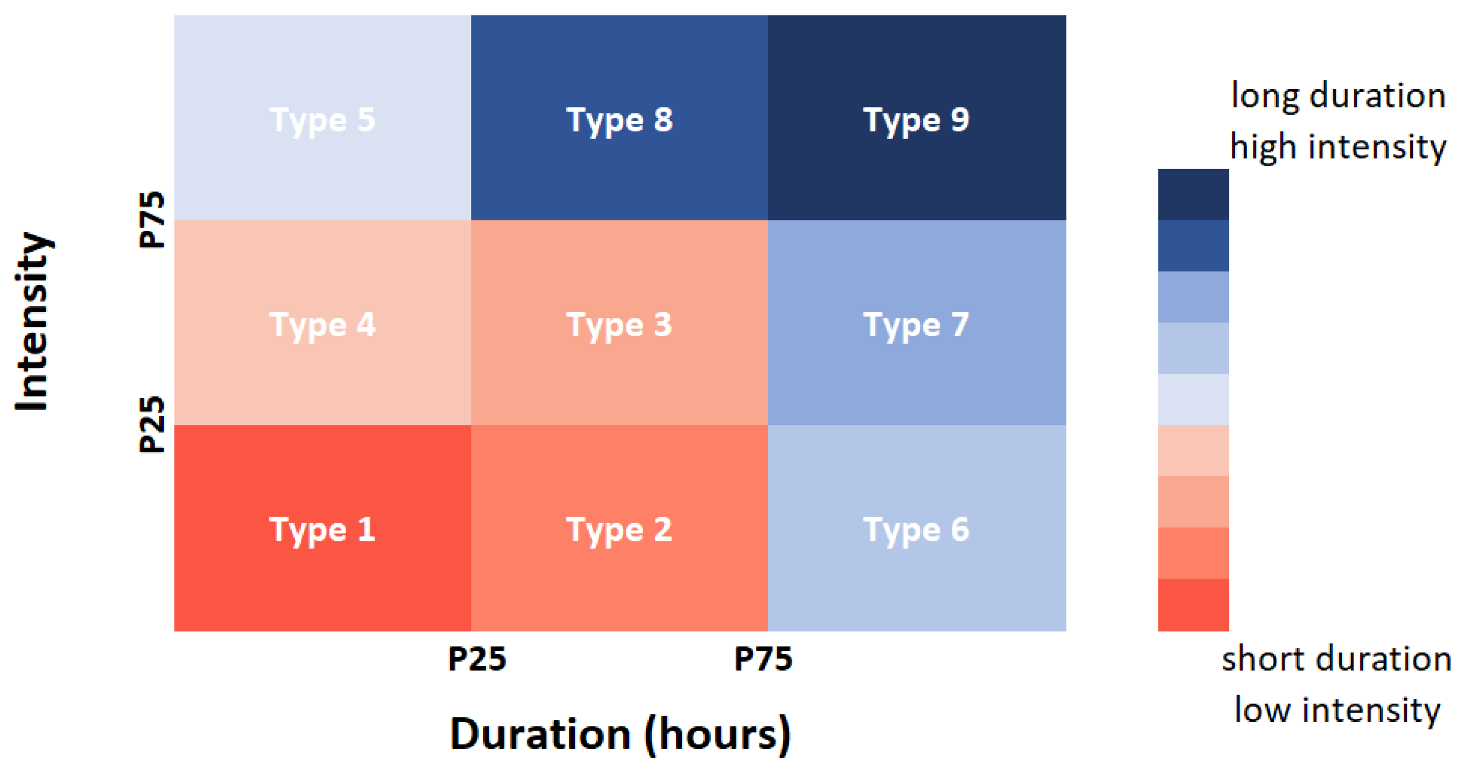
Figure 2.
Matrix of the possible extreme events, considering intensity and duration.
Figure 2.
Matrix of the possible extreme events, considering intensity and duration.
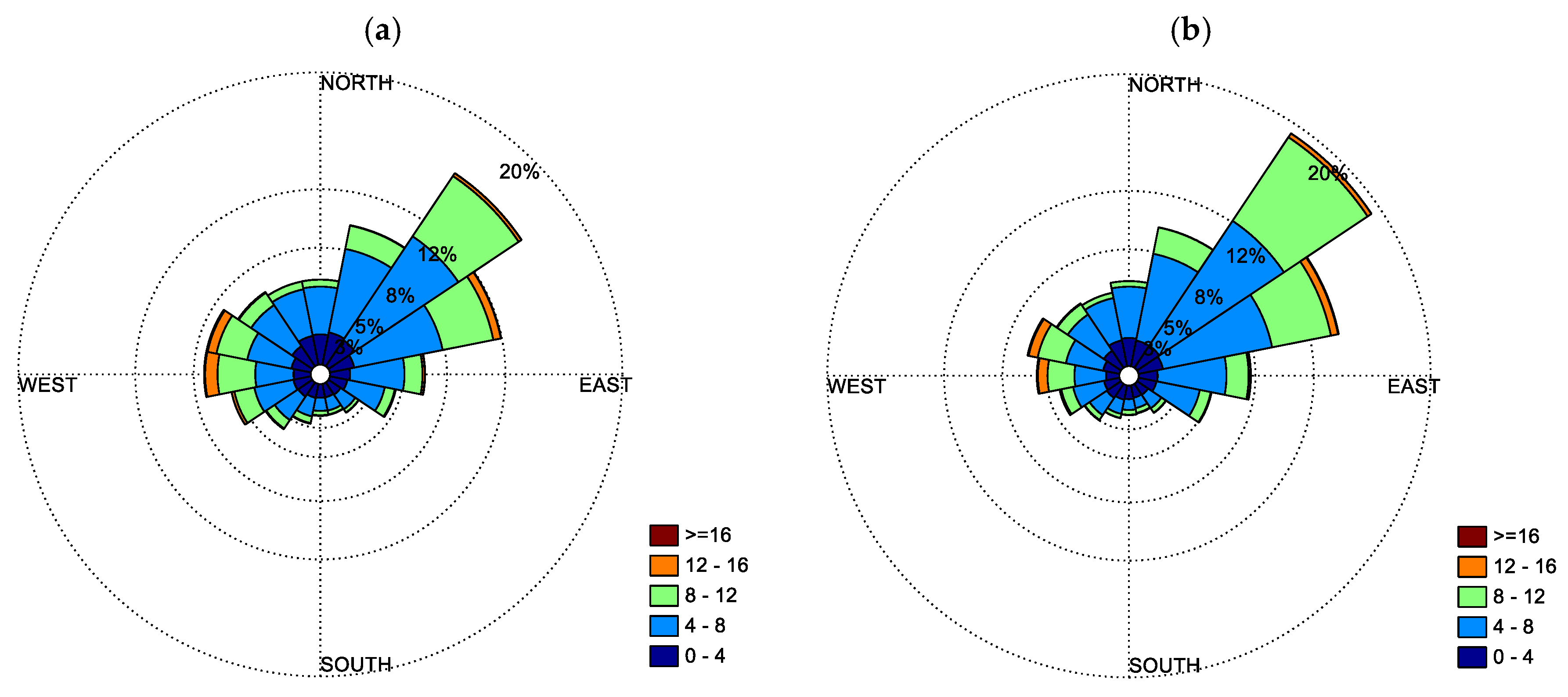
Figure 3.
Wind roses for wind at the surface in Lisboa for (a) historical and (b) future climates. Each colour represents an interval of wind speed. Sixteen directional divisions. The circles mark the number of occurrence (in percentage) for each wind direction (16 direction bars were considered).
Figure 3.
Wind roses for wind at the surface in Lisboa for (a) historical and (b) future climates. Each colour represents an interval of wind speed. Sixteen directional divisions. The circles mark the number of occurrence (in percentage) for each wind direction (16 direction bars were considered).
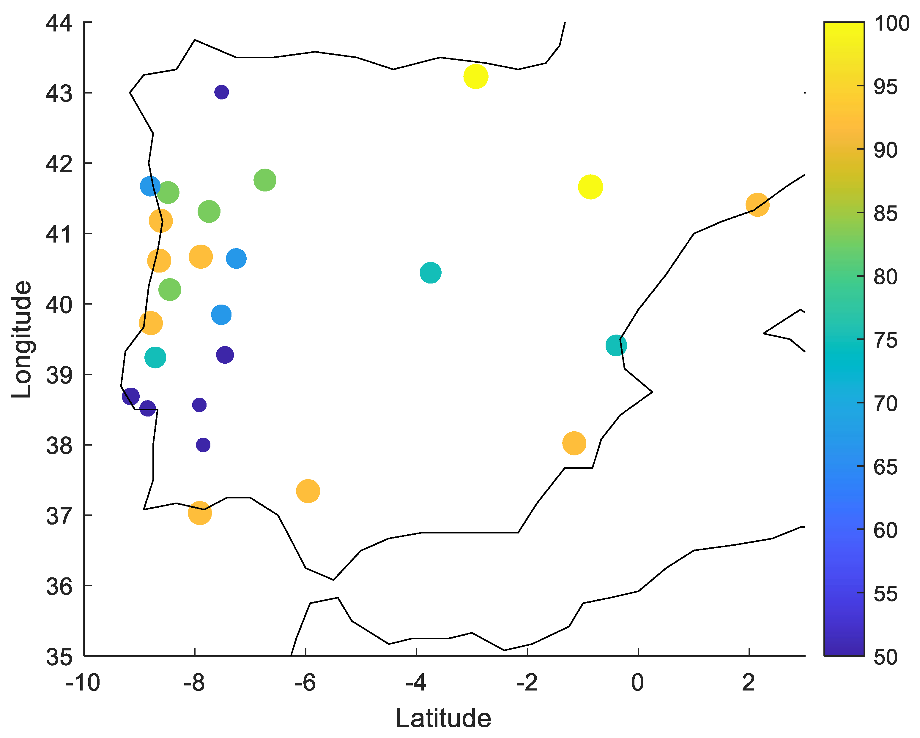
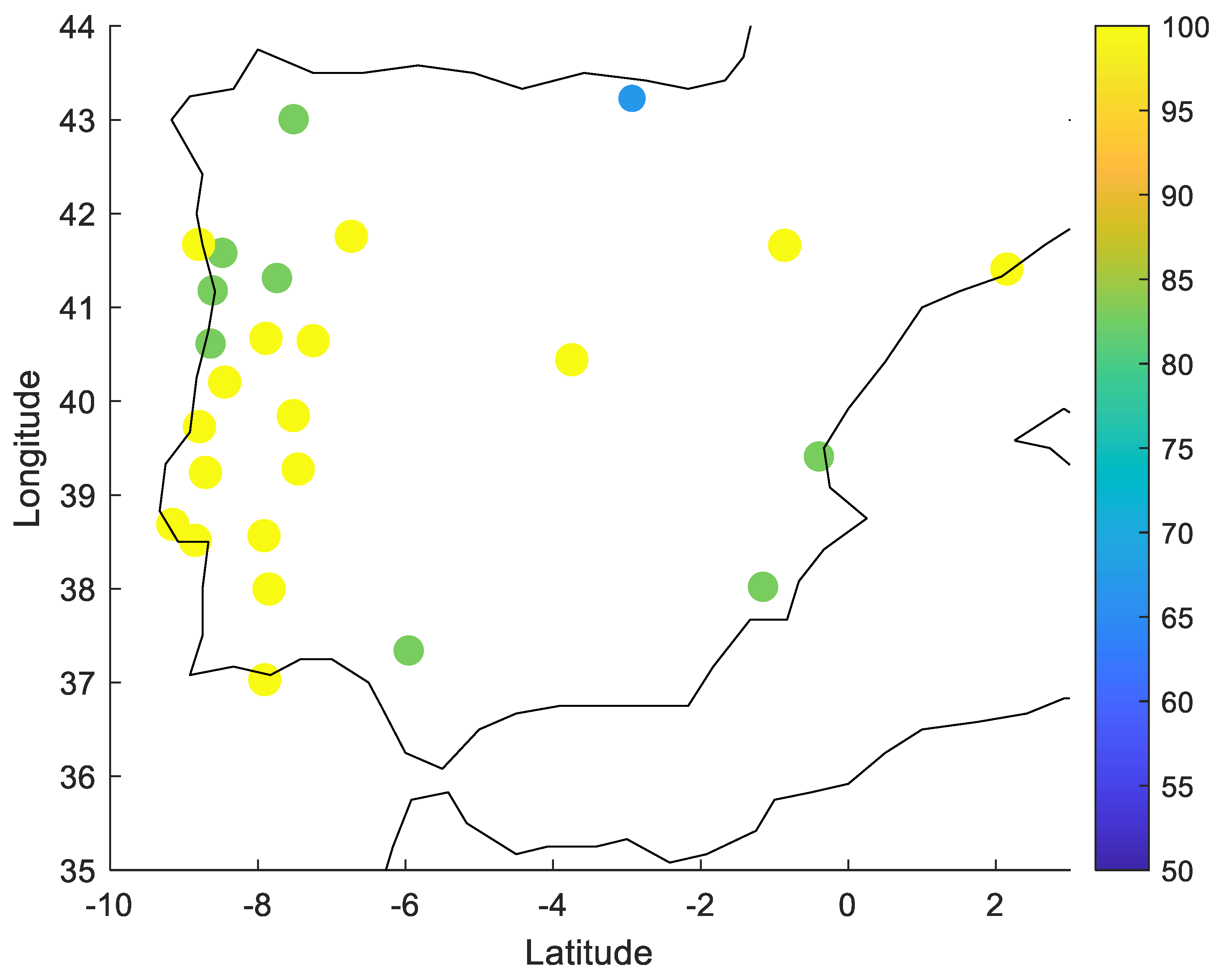
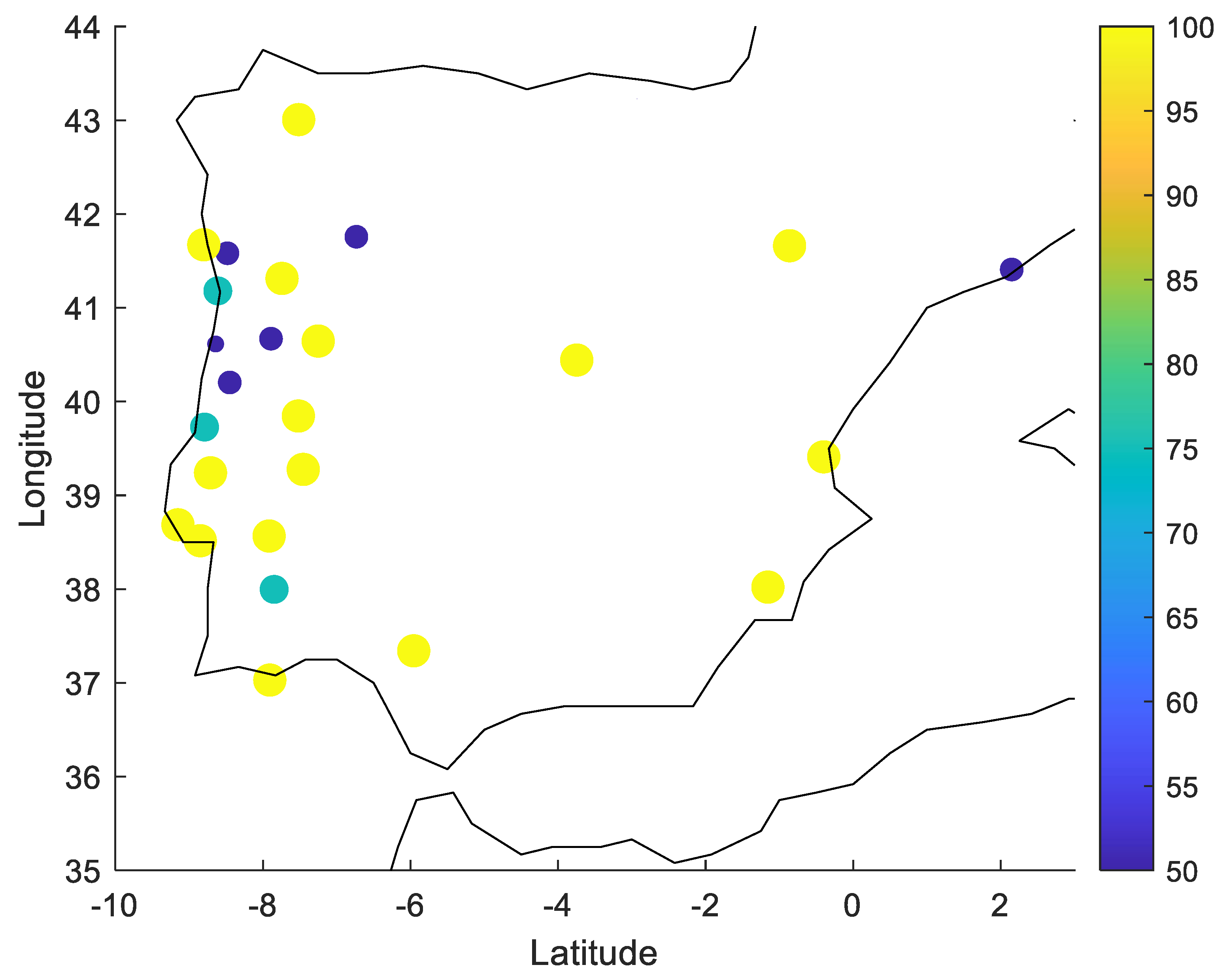
Figure 4.
Average percentage of time in one year that near surface wind speed differences, future minus historic, are negative.
Figure 4.
Average percentage of time in one year that near surface wind speed differences, future minus historic, are negative.
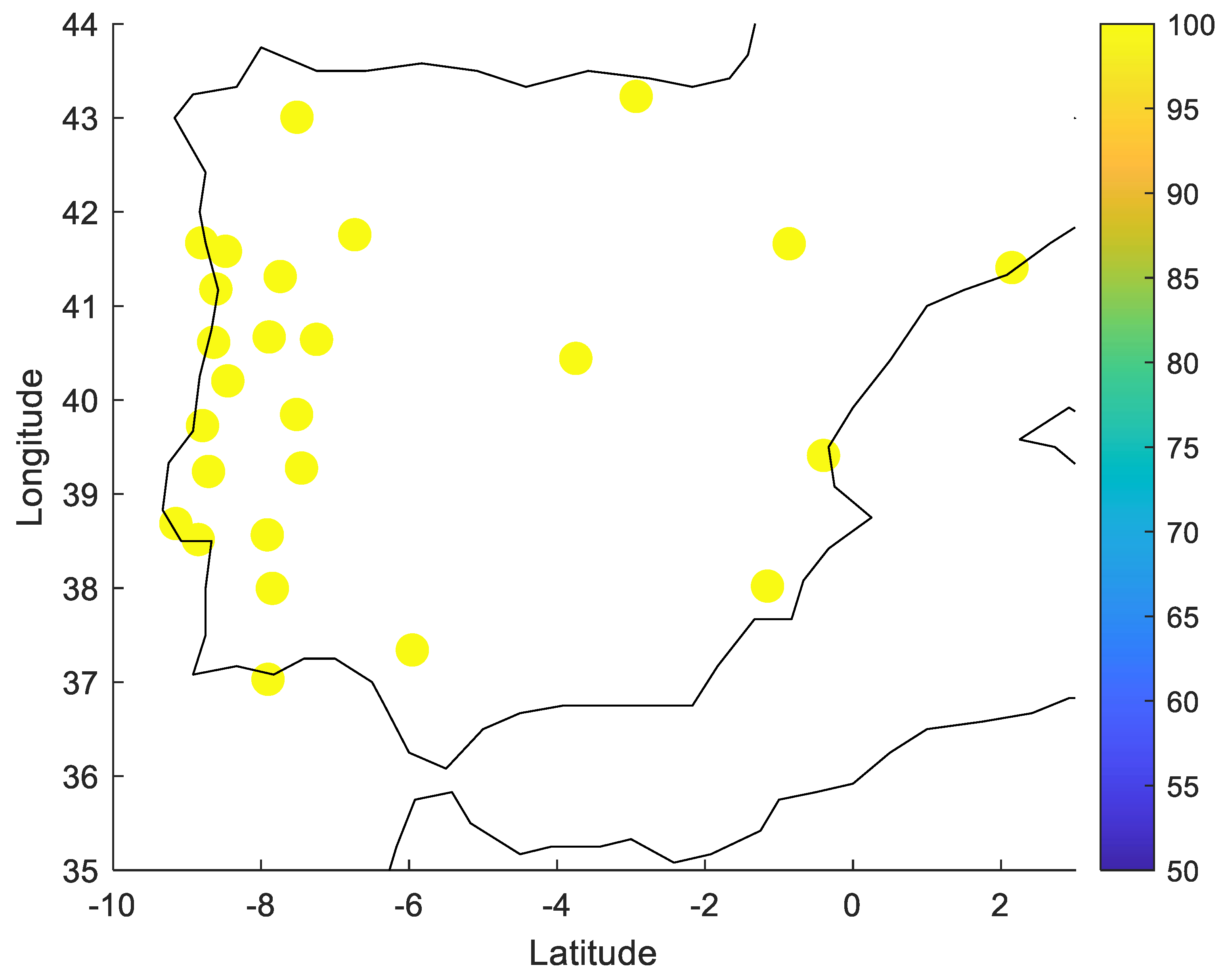
Figure 5.
Average percentage of time for the May–October period that 850 hPa wind speed differences, future minus historic, are negative.
Figure 5.
Average percentage of time for the May–October period that 850 hPa wind speed differences, future minus historic, are negative.
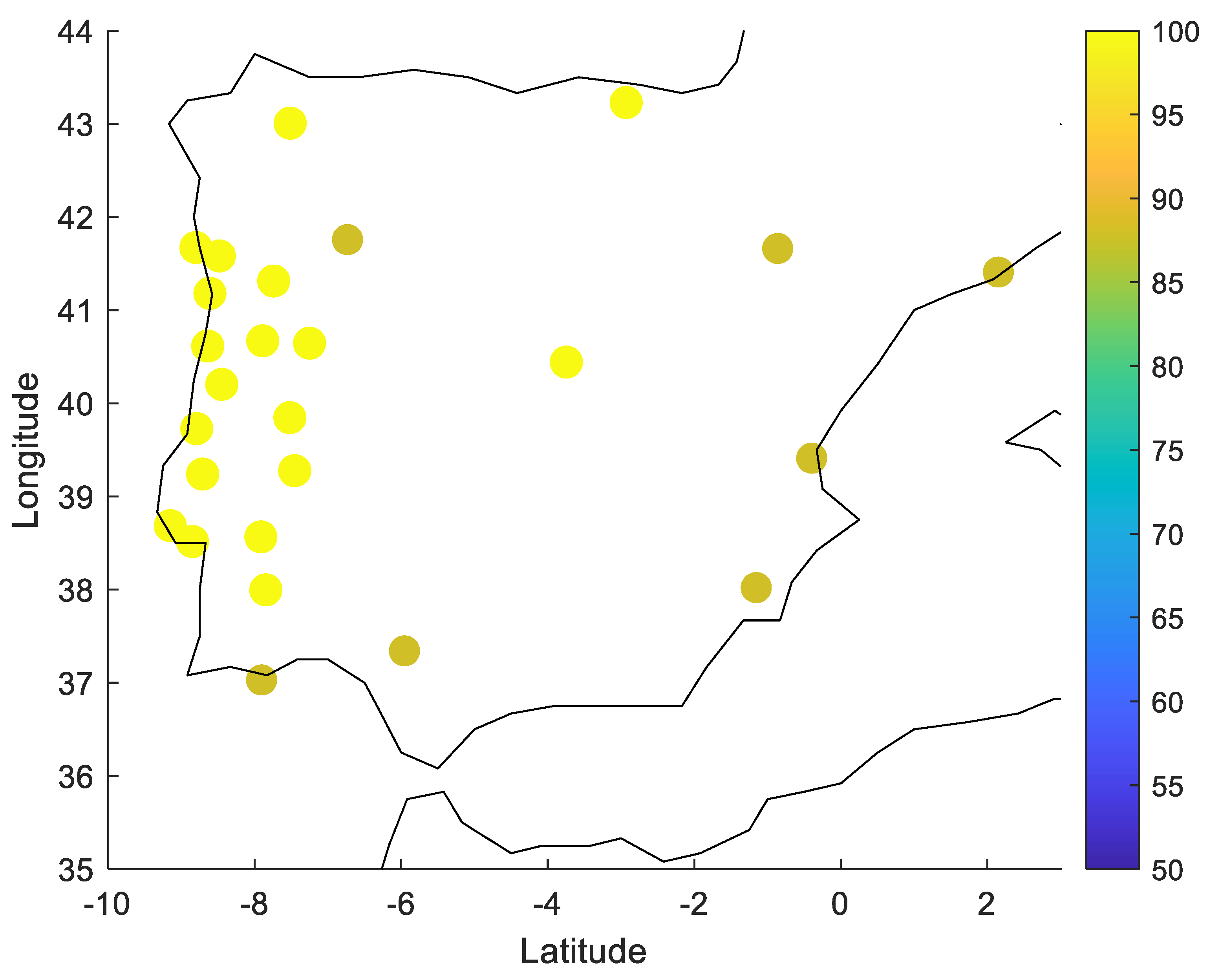
Figure 6.
Average percentage of time for the July–September period that 300 hPa wind speed differences, future minus historic, are negative.
Figure 6.
Average percentage of time for the July–September period that 300 hPa wind speed differences, future minus historic, are negative.
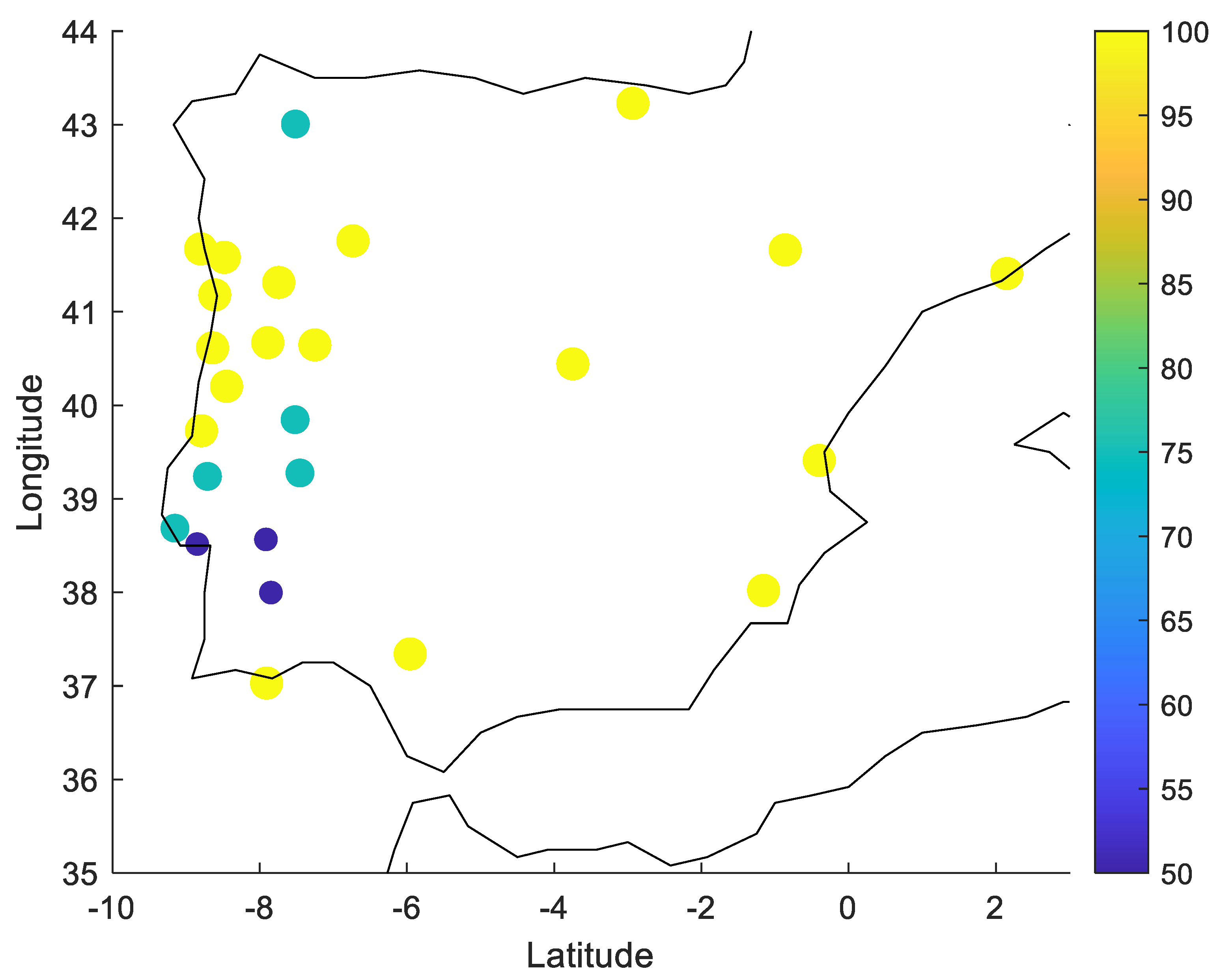
Figure 7.
Average percentage of time for the November–June period that wind shear 0–6 km differences, future minus historic, are positive.
Figure 7.
Average percentage of time for the November–June period that wind shear 0–6 km differences, future minus historic, are positive.
Figure 8.
Average percentage of time for the July–October period that wind shear 0–6 km differences, future minus historic, are negative.
Figure 8.
Average percentage of time for the July–October period that wind shear 0–6 km differences, future minus historic, are negative.
Figure 9.
Average percentage of time for the June–September period that storm-relative helicity (SRH) 0–3 km differences, future minus historic, are positive.
Figure 9.
Average percentage of time for the June–September period that storm-relative helicity (SRH) 0–3 km differences, future minus historic, are positive.
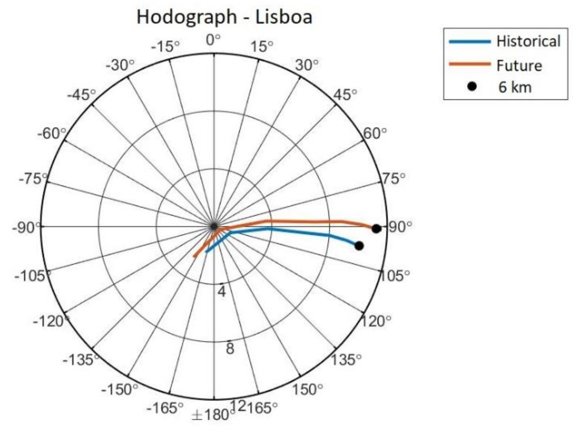
Figure 10.
Hodograph for Lisboa, from 0 to 6 km, for historical (blue line) and future (orange line) climates.
Figure 10.
Hodograph for Lisboa, from 0 to 6 km, for historical (blue line) and future (orange line) climates.
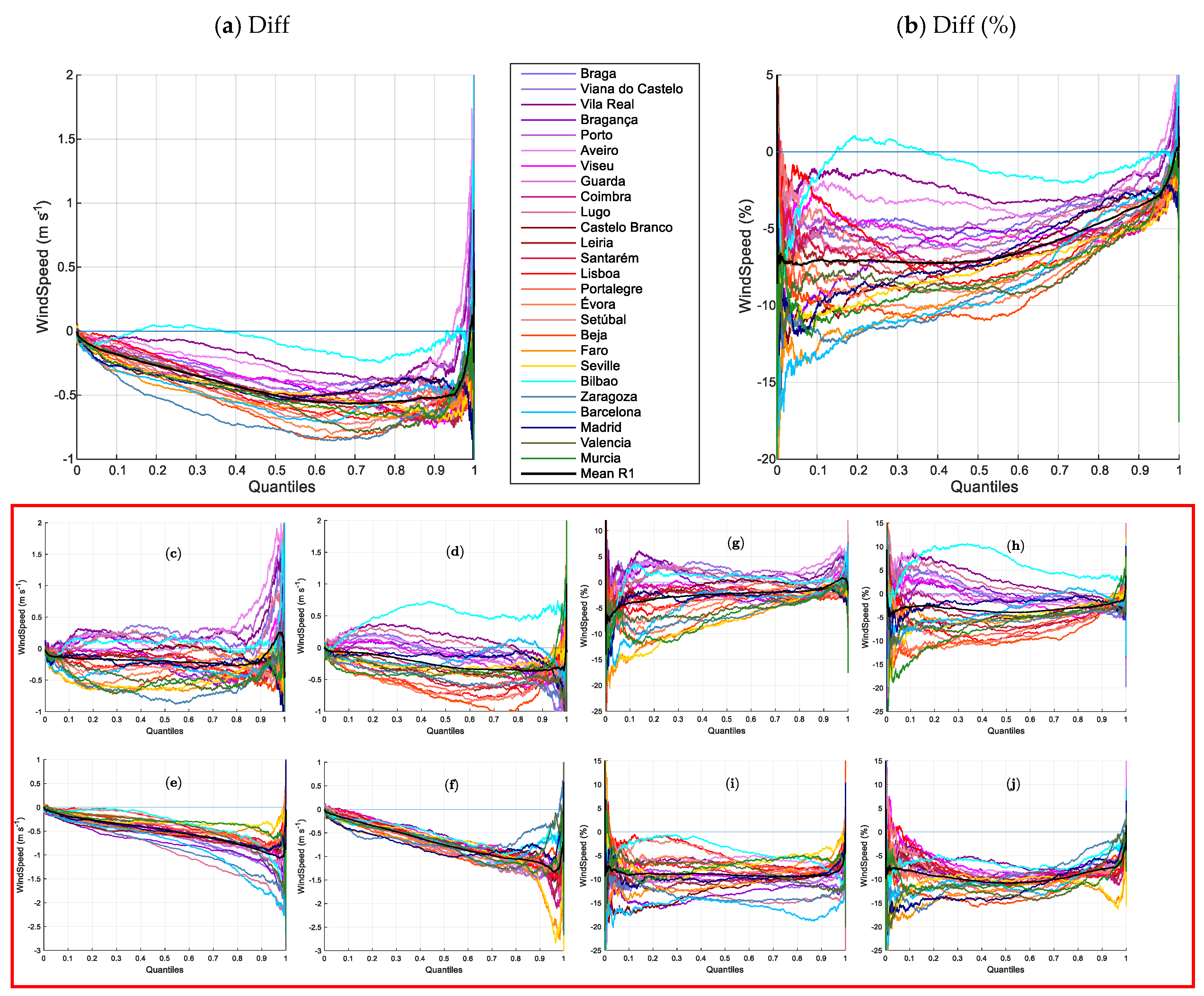
Figure 11.
Differences (future-historic) for wind speed at 850 hPa for annual and seasonal conditions, as a function of the quantiles of the corresponding empirical distributions. (a) Absolute differences (m s−1) and (b) relative percentual differences (%). Seasonal absolute differences are also represented for (c) winter, (d) spring, (e) summer and (f) autumn, and Seasonal percentual differences for (g) winter, (h) spring, (i) summer and (j) autumn. The black line (Mean R1) refers to the mean of region 1 (total area).
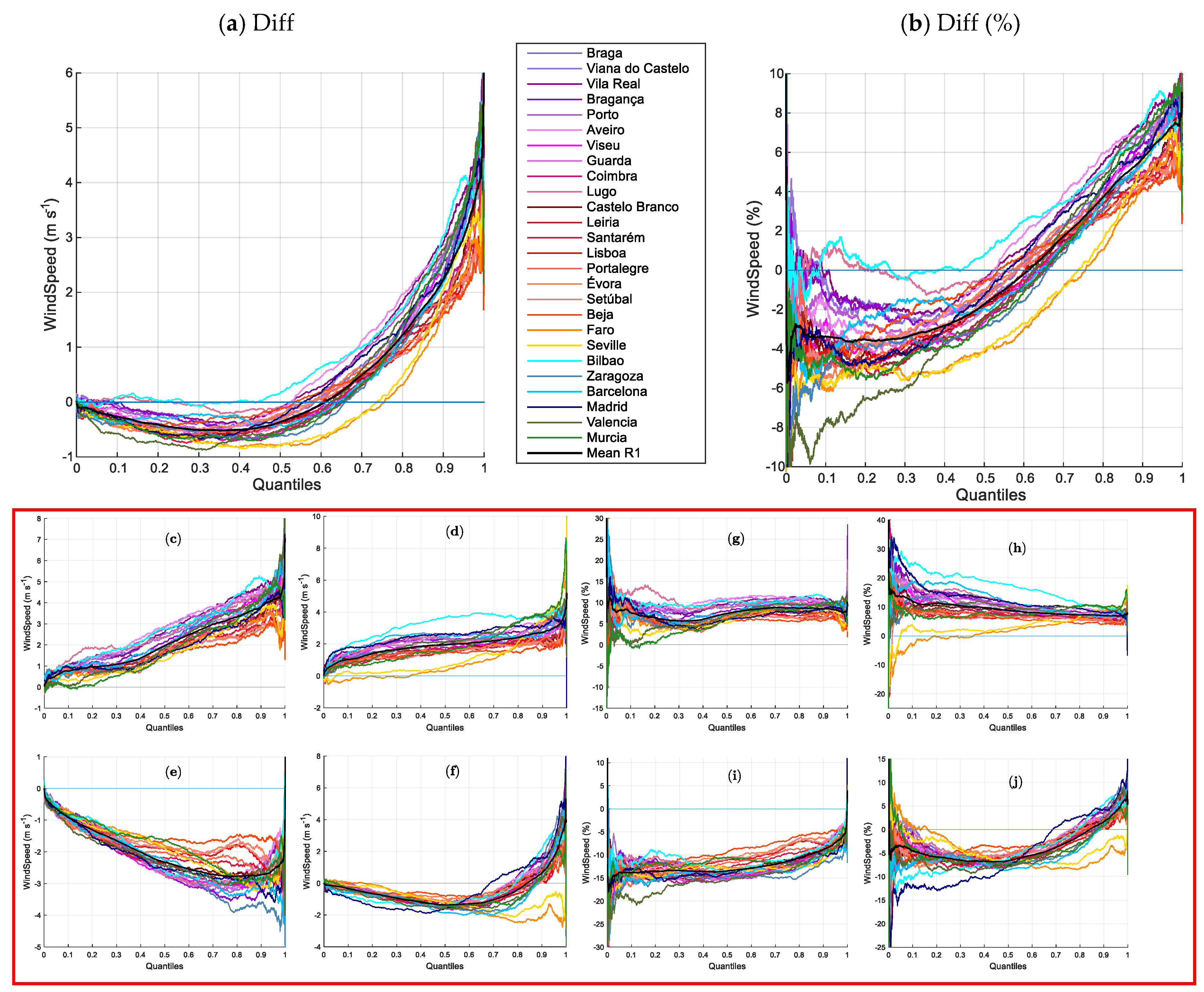
Figure 12.
Differences (future-historic) for wind speed at 300 hPa for annual and seasonal conditions, as a function of the quantiles of the corresponding empirical distributions. (a) Absolute differences (m s−1) and (b) relative percentual differences (%). Seasonal absolute differences are also represented for (c) winter, (d) spring, (e) summer and (f) autumn, and Seasonal percentual differences for (g) winter, (h) spring, (i) summer and (j) autumn. The black line (Mean R1) refers to the mean of region 1 (total area).
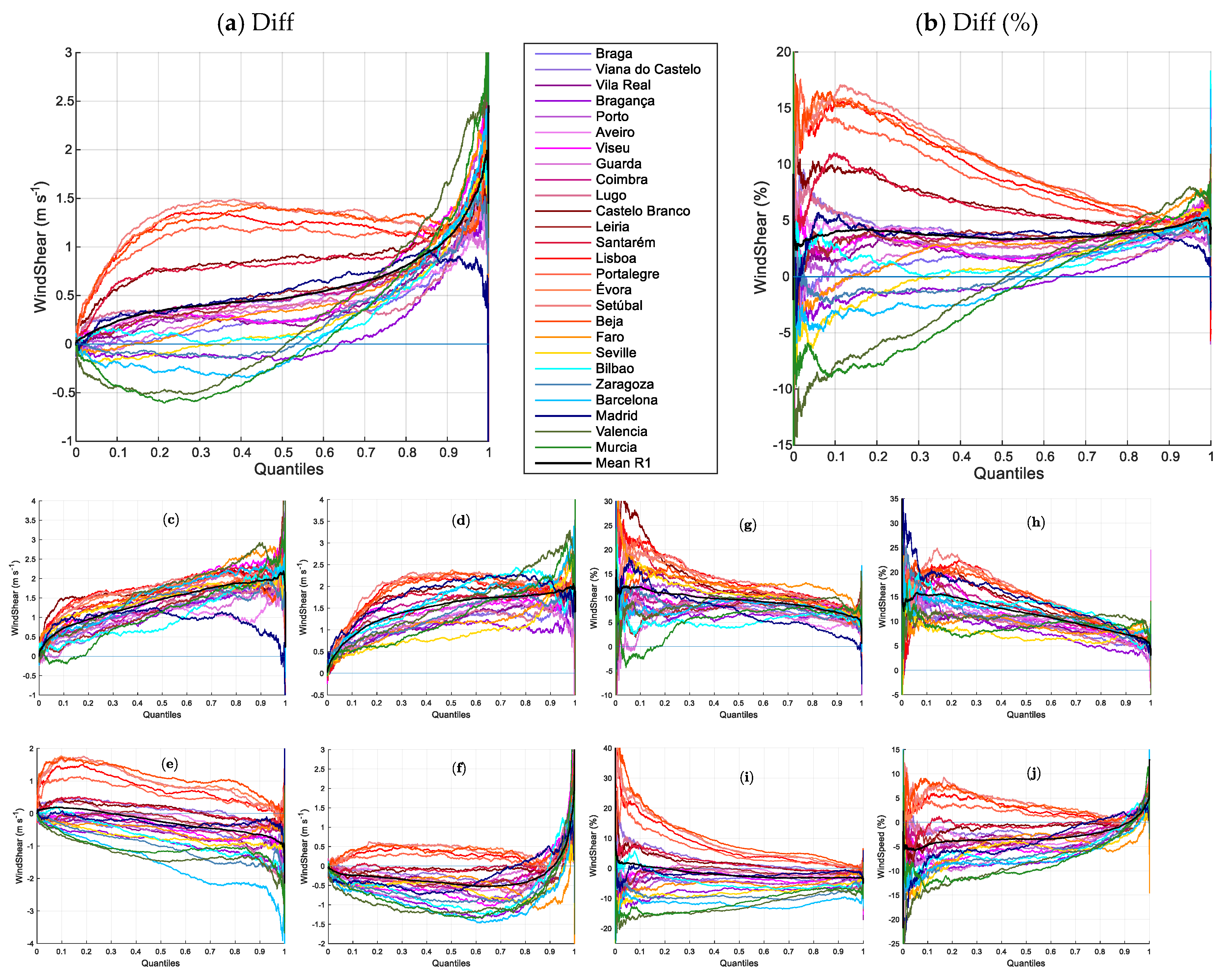
Figure 13.
Differences (future-historic) for wind shear 0–6 km for annual and seasonal conditions, as a function of the quantiles of the corresponding empirical distributions. (a) Absolute differences (m s−1) and (b) relative percentual differences (%). Seasonal absolute differences are also represented for (c) winter, (d) spring, (e) summer and (f) autumn, and Seasonal percentual differences for (g) winter, (h) spring, (i) summer and (j) autumn.The black line (Mean R1) refers to the mean of region 1 (total area).
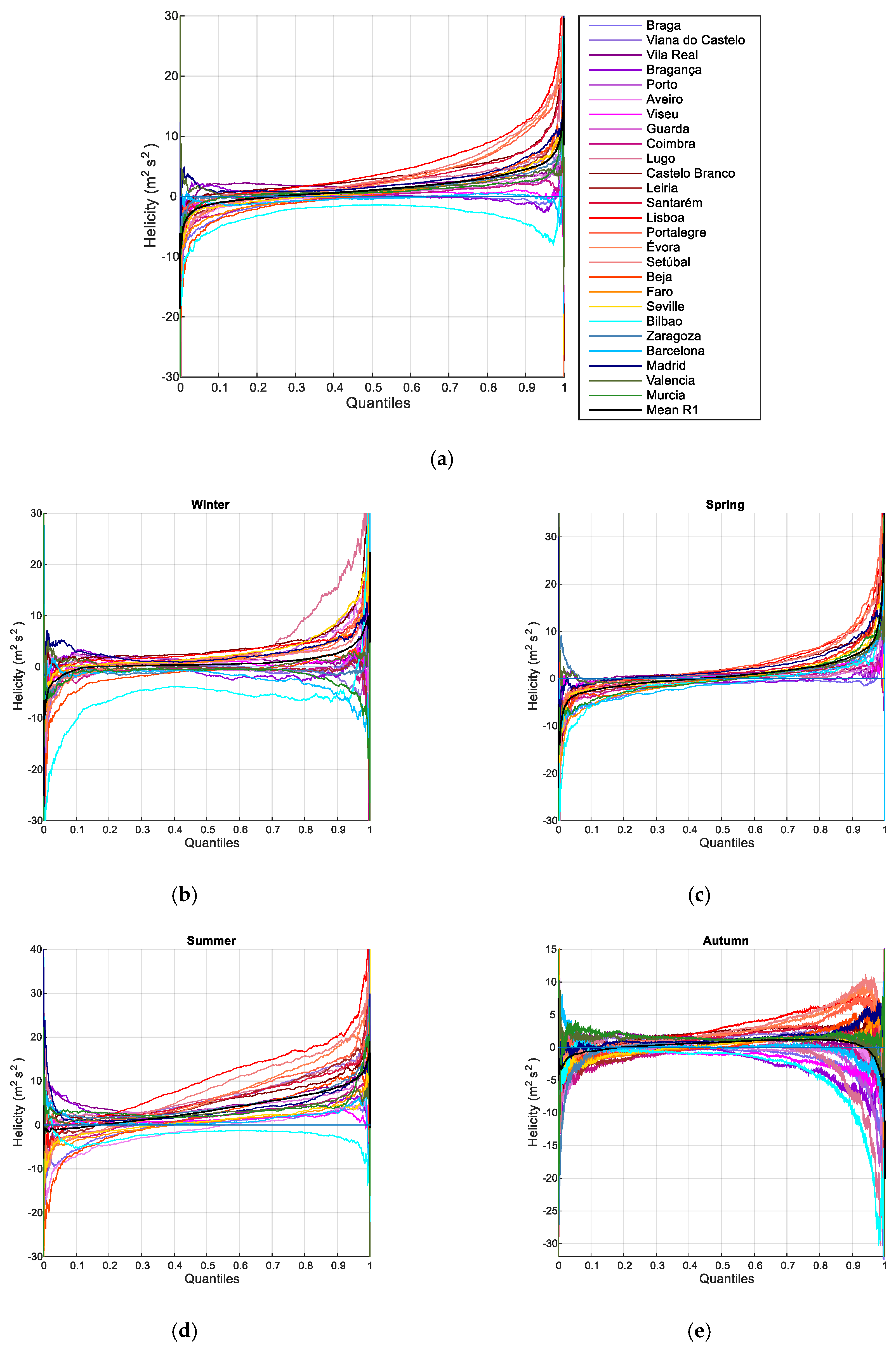
Figure 14.
Absolute differences (m2 s2, future-historic) for helicity 0–3 km for annual and seasonal conditions, as a function of the quantiles of the corresponding empirical distributions. The black line (Mean R1) refers to the mean of region 1 (total area). (a) annual, (b) winter, (c) spring, (d) summer, (e) winter.
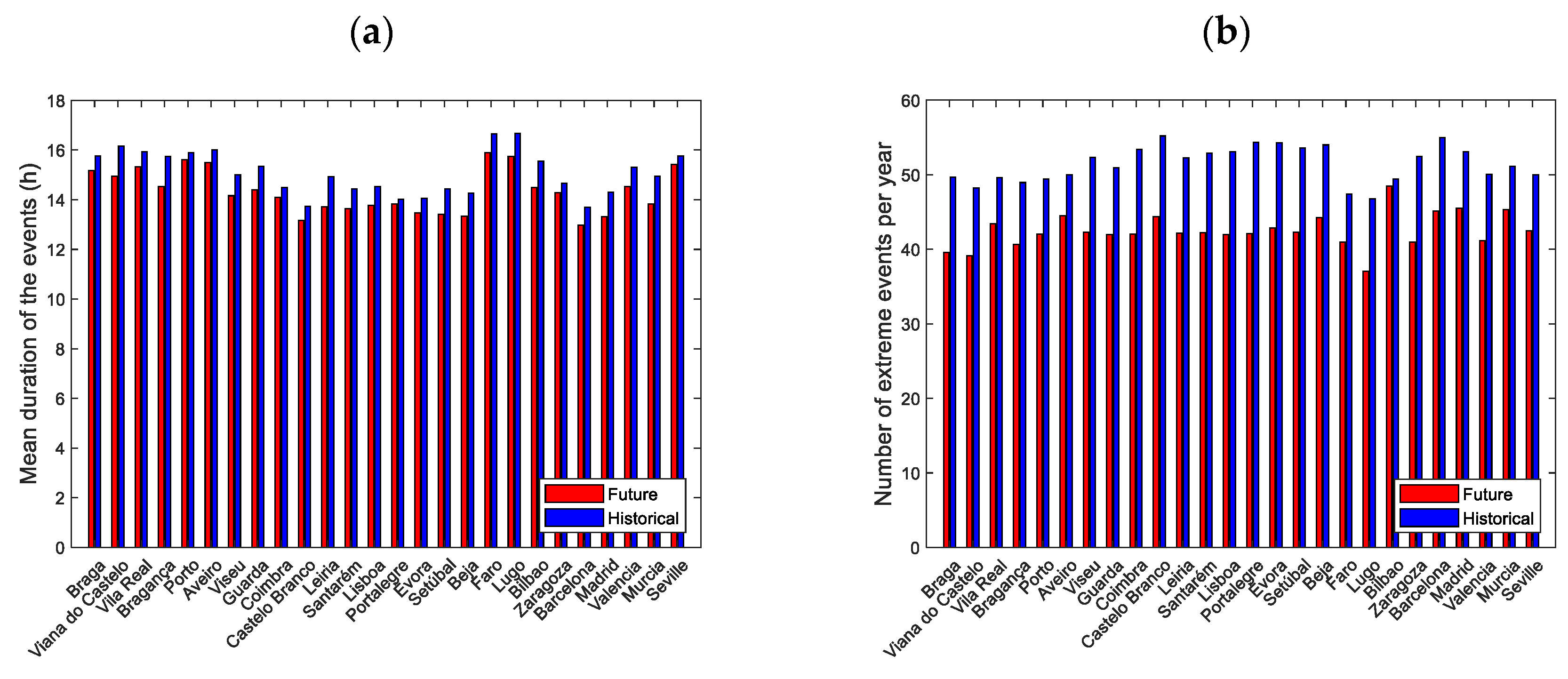
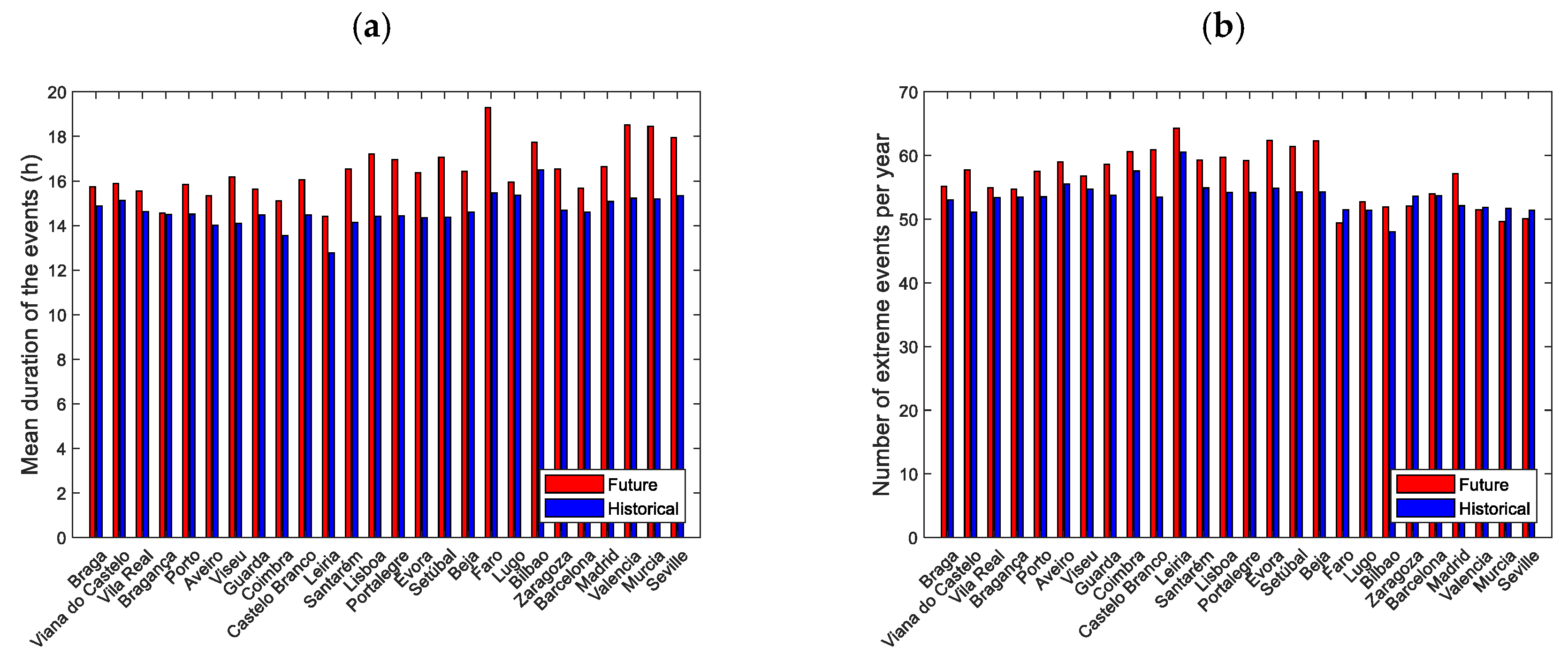
Figure 15.
(a) Mean duration (hours) of the extreme events of the wind speed at 850 hPa and (b) the number of extreme events per year, for both the historical (blue) and future (red) climates and all cities.
Figure 15.
(a) Mean duration (hours) of the extreme events of the wind speed at 850 hPa and (b) the number of extreme events per year, for both the historical (blue) and future (red) climates and all cities.
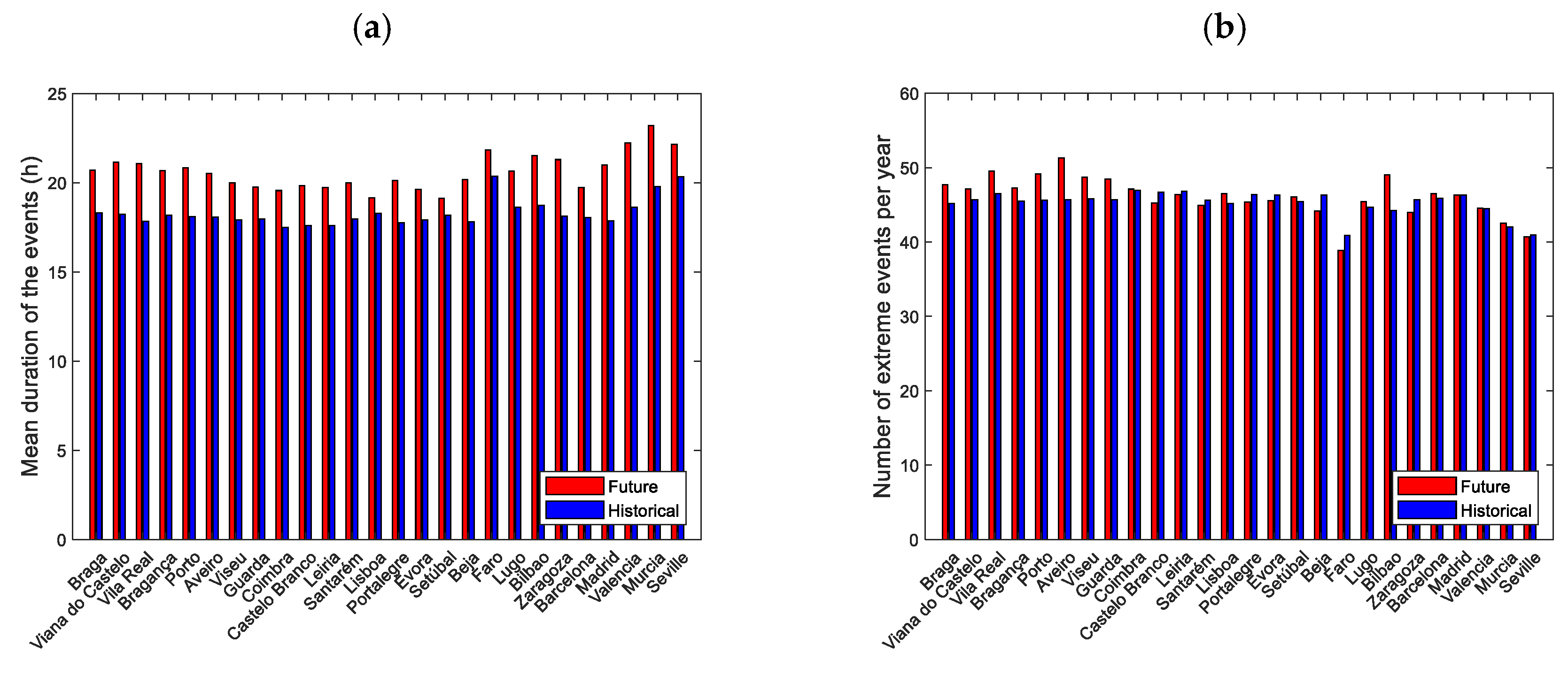
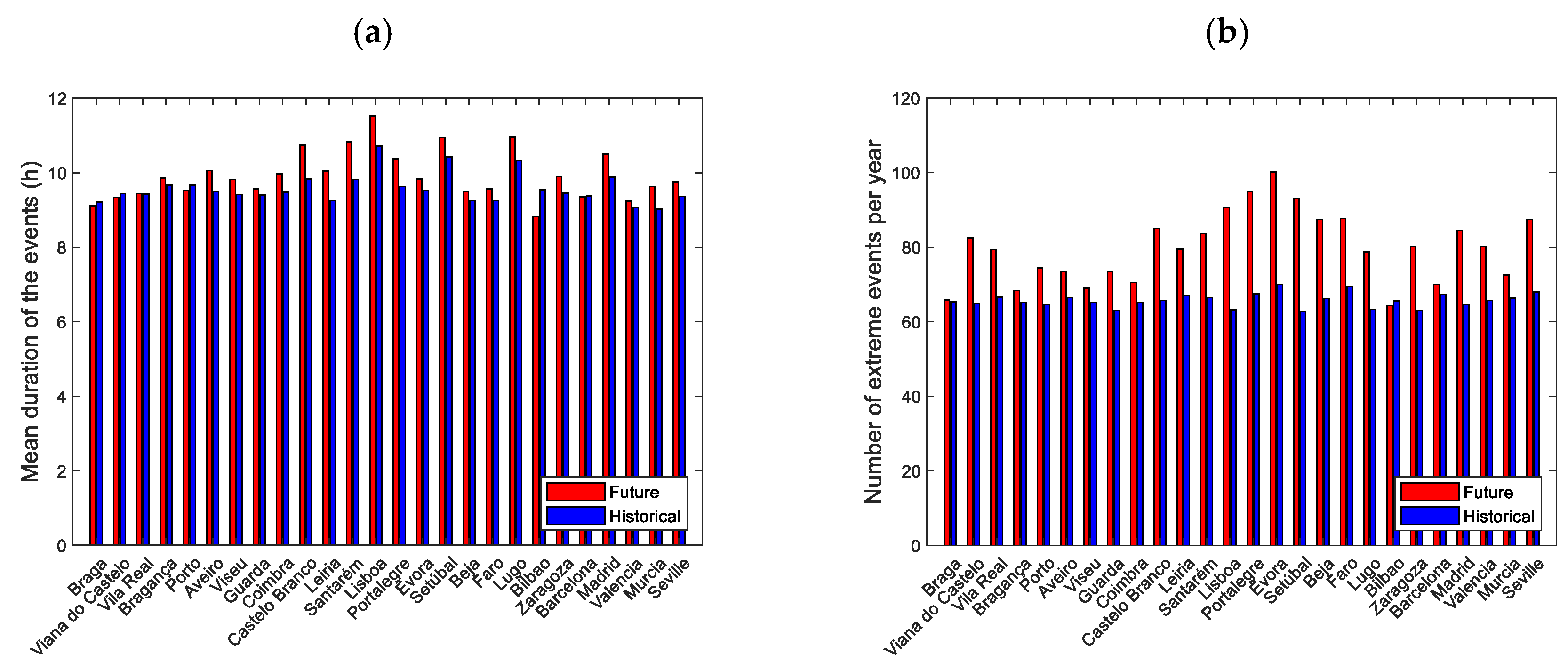
Figure 16.
(a) Mean duration (hours) of extreme events of the wind speed at 300 hPa and (b) the number of extreme events per year, for historical (blue) and future (red) climates and for all cities.
Figure 16.
(a) Mean duration (hours) of extreme events of the wind speed at 300 hPa and (b) the number of extreme events per year, for historical (blue) and future (red) climates and for all cities.
Figure 17.
(a) Mean duration (hours) of the extreme events of the wind shear and (b) number of extreme events per year, for historical (blue) and future (red) climates for all cities.
Figure 17.
(a) Mean duration (hours) of the extreme events of the wind shear and (b) number of extreme events per year, for historical (blue) and future (red) climates for all cities.
Figure 18.
(a) Mean duration (hours) of the extreme events of the helicity and (b) number of extreme events per year, for historical (blue) and future (red) climates for all cities.
Figure 18.
(a) Mean duration (hours) of the extreme events of the helicity and (b) number of extreme events per year, for historical (blue) and future (red) climates for all cities.
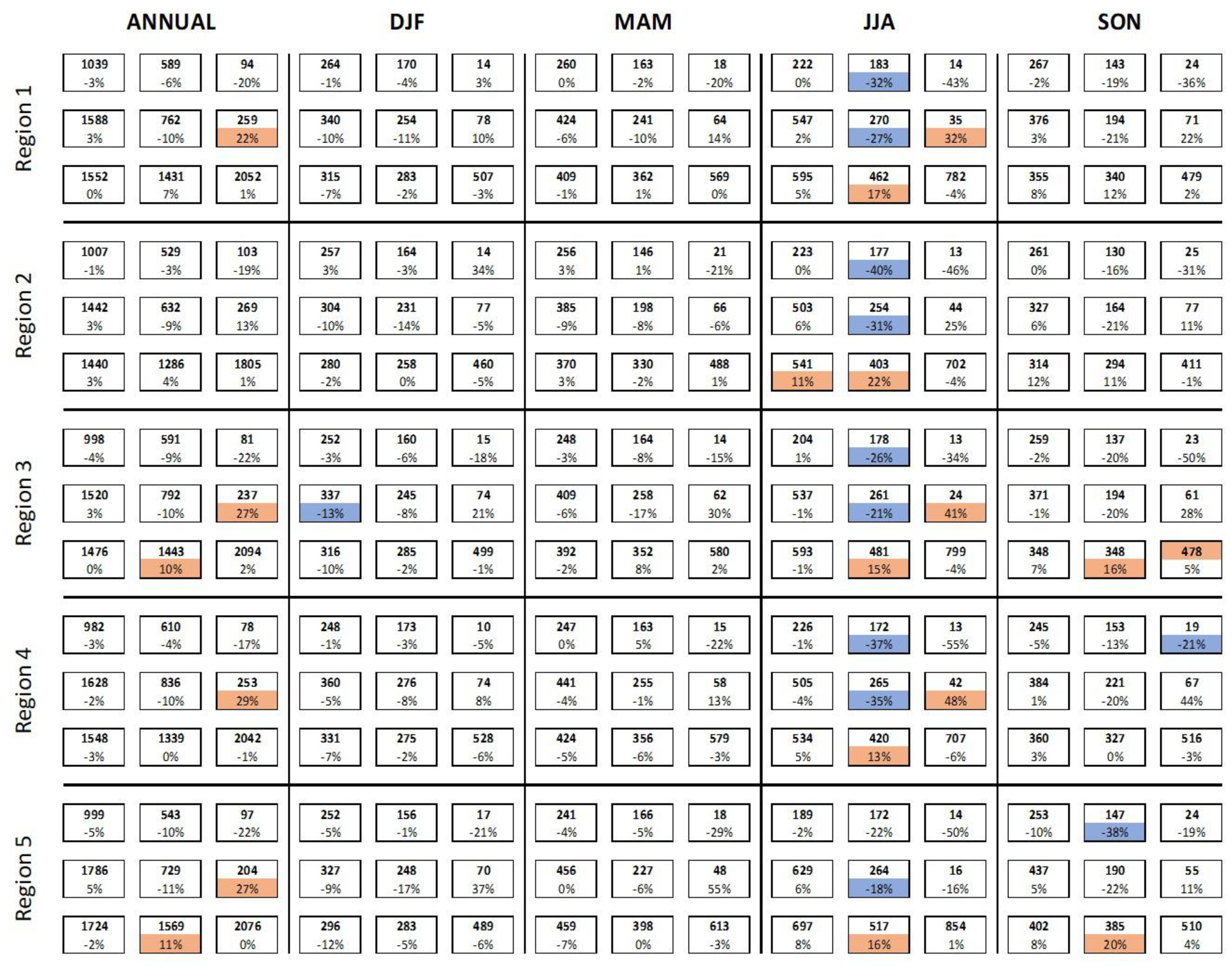
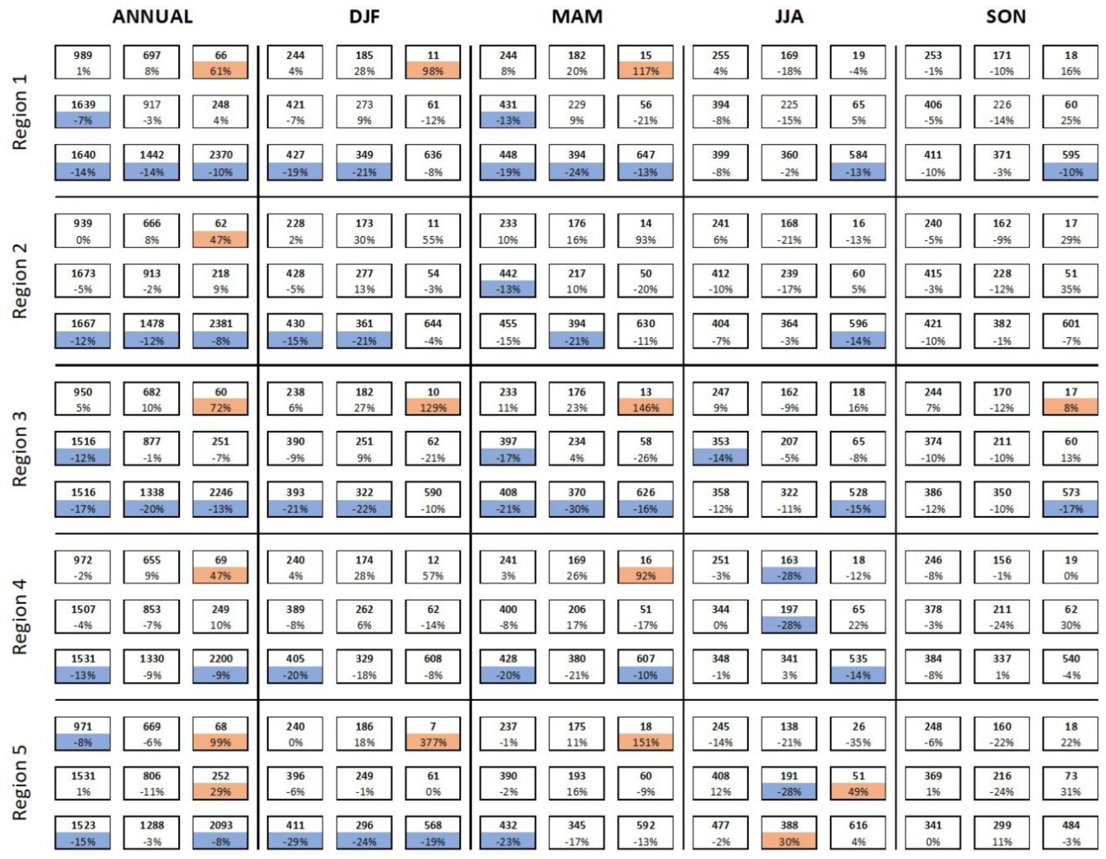
Figure 19.
The number of wind speed events at 850 hPa for each type of event, region and season. For the historical climate (1st line of the cell) and the difference between the future and historical (2nd line of the cell). Shaded values indicate significant differences (t-student 5%) positive (red) and negative (blue).
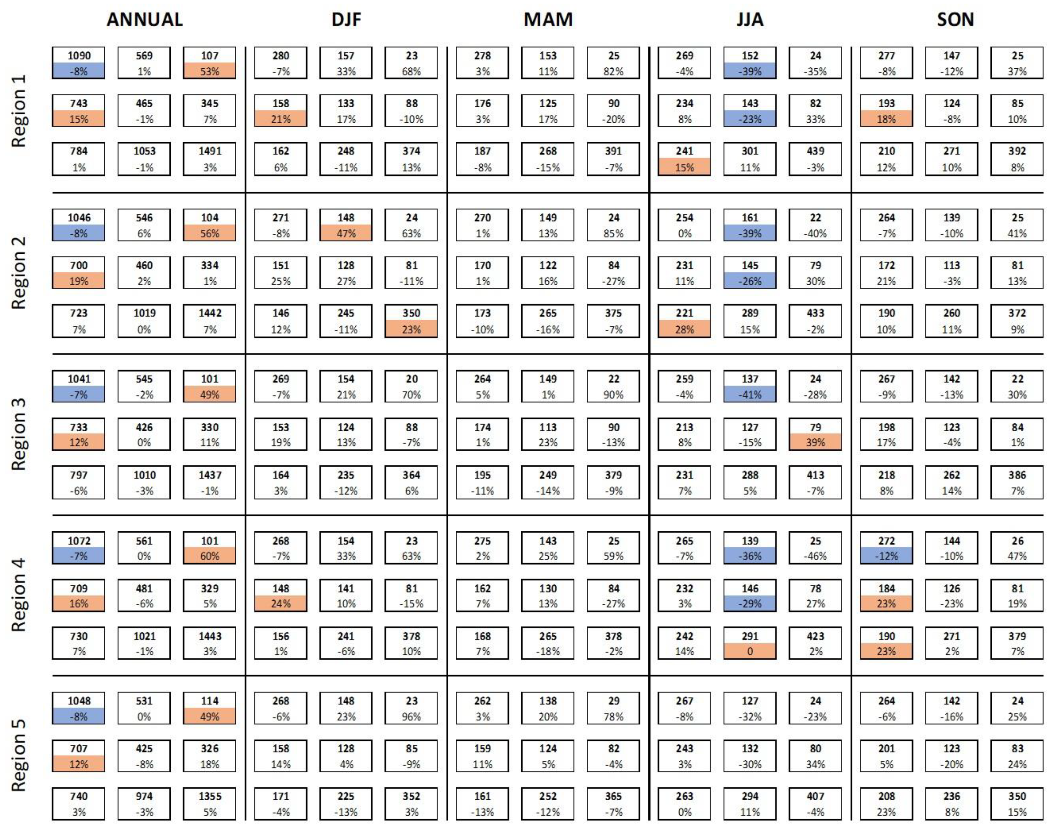
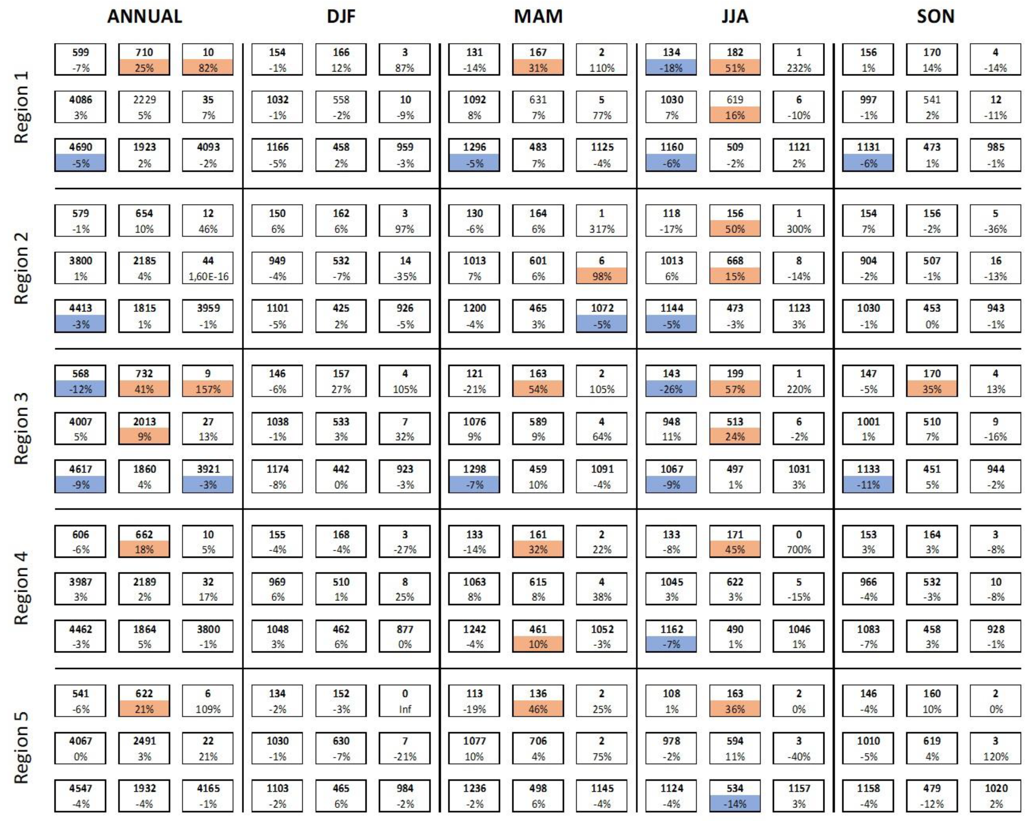
Figure 20.
The number of wind speed events at 300 hPa for each type of event, region and season. For the historical climate (1st line of the cell) and the difference between the future and historical (2nd line of the cell). Shaded values indicate significant differences (t-student 5%) positive (red) and negative (blue).
Figure 21.
The number of events of the wind shear intensity between 0 and 6 km for each type of event, region and season. For the historical climate (1st line of the cell) and the difference between the future and historical (2nd line of the cell). Shaded values indicate significant differences (t-student 5%) positive (red) and negative (blue).
Figure 22.
The number of events of helicity between 0 and 3 km for each type of event, region and season. For the historical climate (1st line of the cell) and the difference between the future and historical (2nd line of the cell). Shaded values indicate significant differences (t-student 5%) positive (red) and negative (blue).
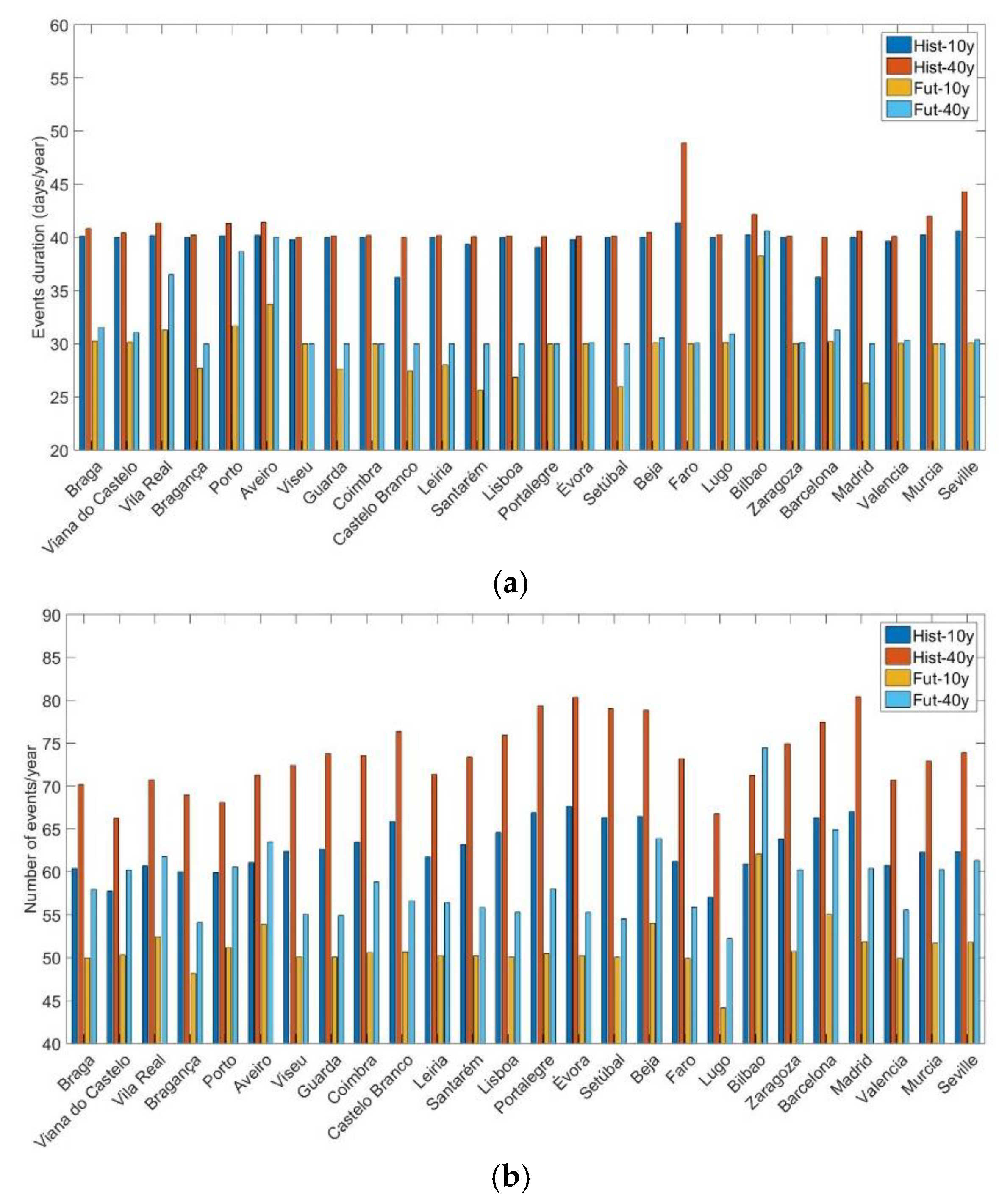
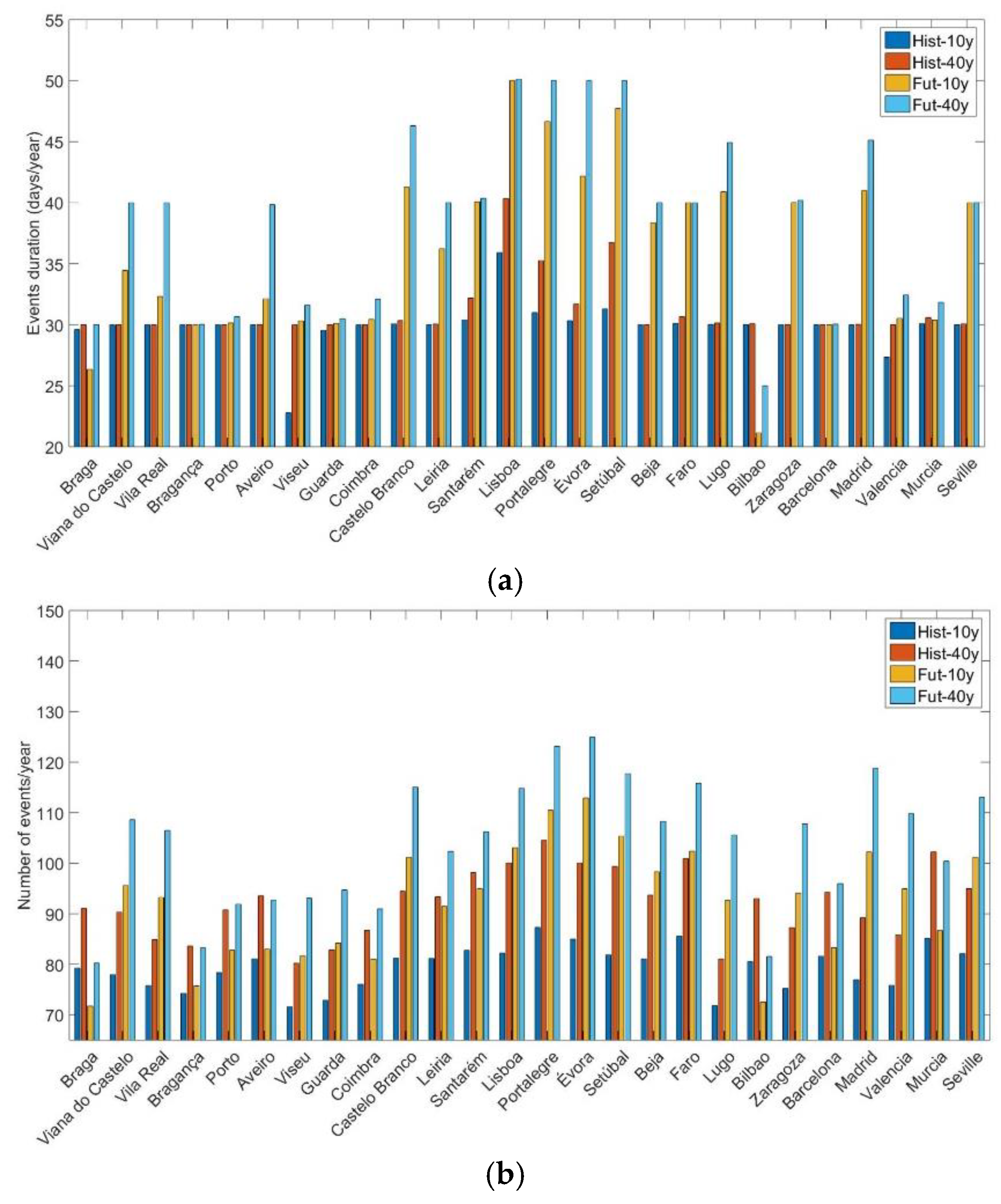
Figure 23.
Comparison of the (a) event duration (days/year) and (b) the number of events (year) in the historical (blue) and future (red) period for extreme events with a return period of 10 years (full line) and 40 years (dashed line) for wind speed at 850 hPa.
Figure 23.
Comparison of the (a) event duration (days/year) and (b) the number of events (year) in the historical (blue) and future (red) period for extreme events with a return period of 10 years (full line) and 40 years (dashed line) for wind speed at 850 hPa.
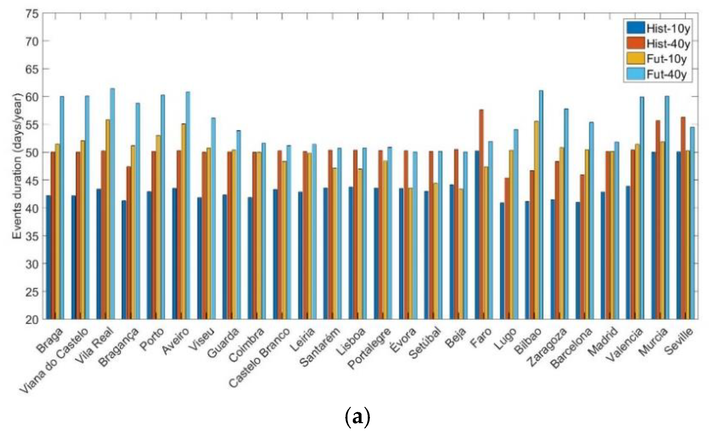
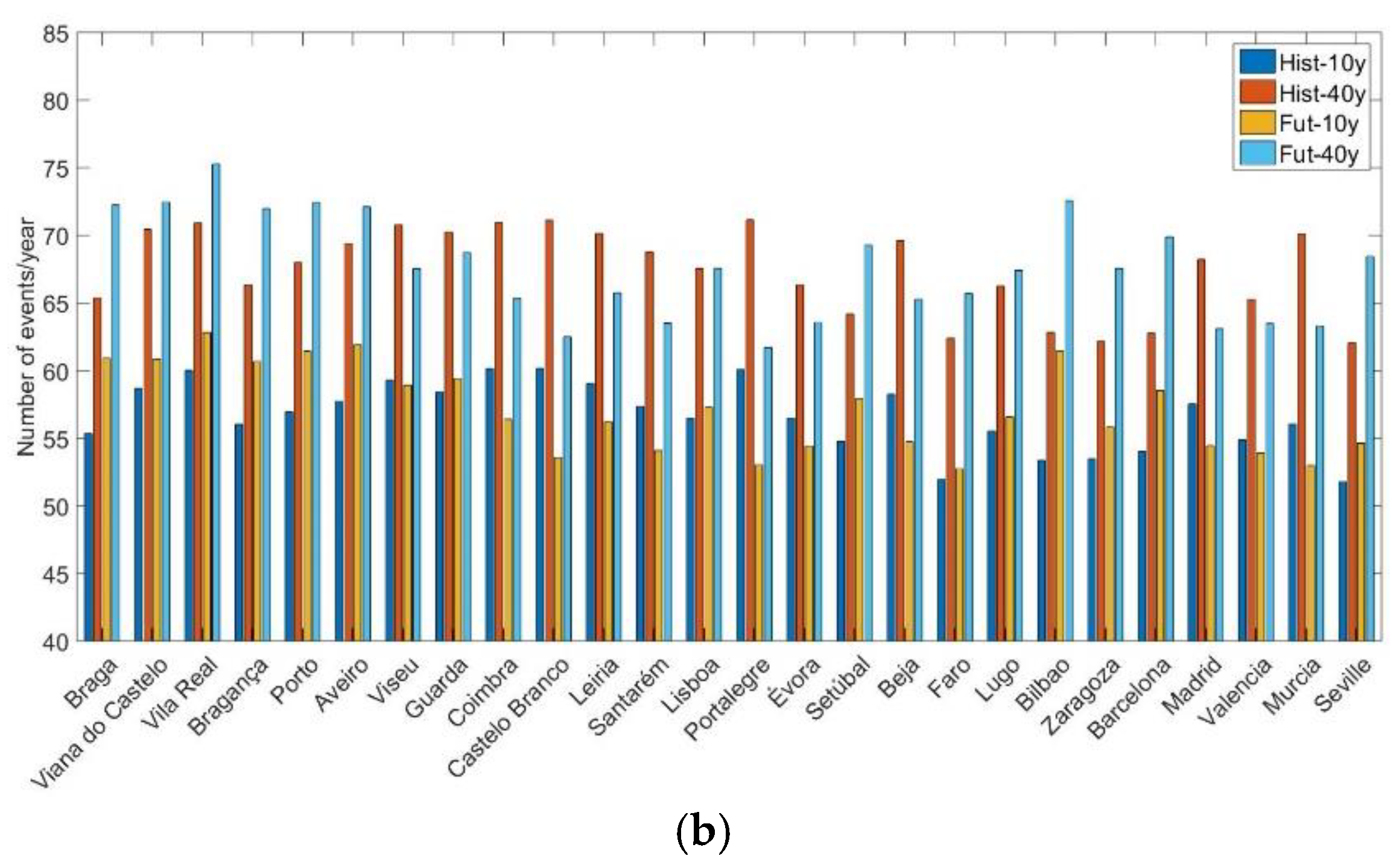
Figure 24.
Comparison of the (a) event duration (days/year) and (b) the number of events (year) in the historical (blue) and future (red) period for extreme events with a return period of 10 years (full line) and 40 years (dashed line) for wind speed at 300 hPa.
Figure 24.
Comparison of the (a) event duration (days/year) and (b) the number of events (year) in the historical (blue) and future (red) period for extreme events with a return period of 10 years (full line) and 40 years (dashed line) for wind speed at 300 hPa.
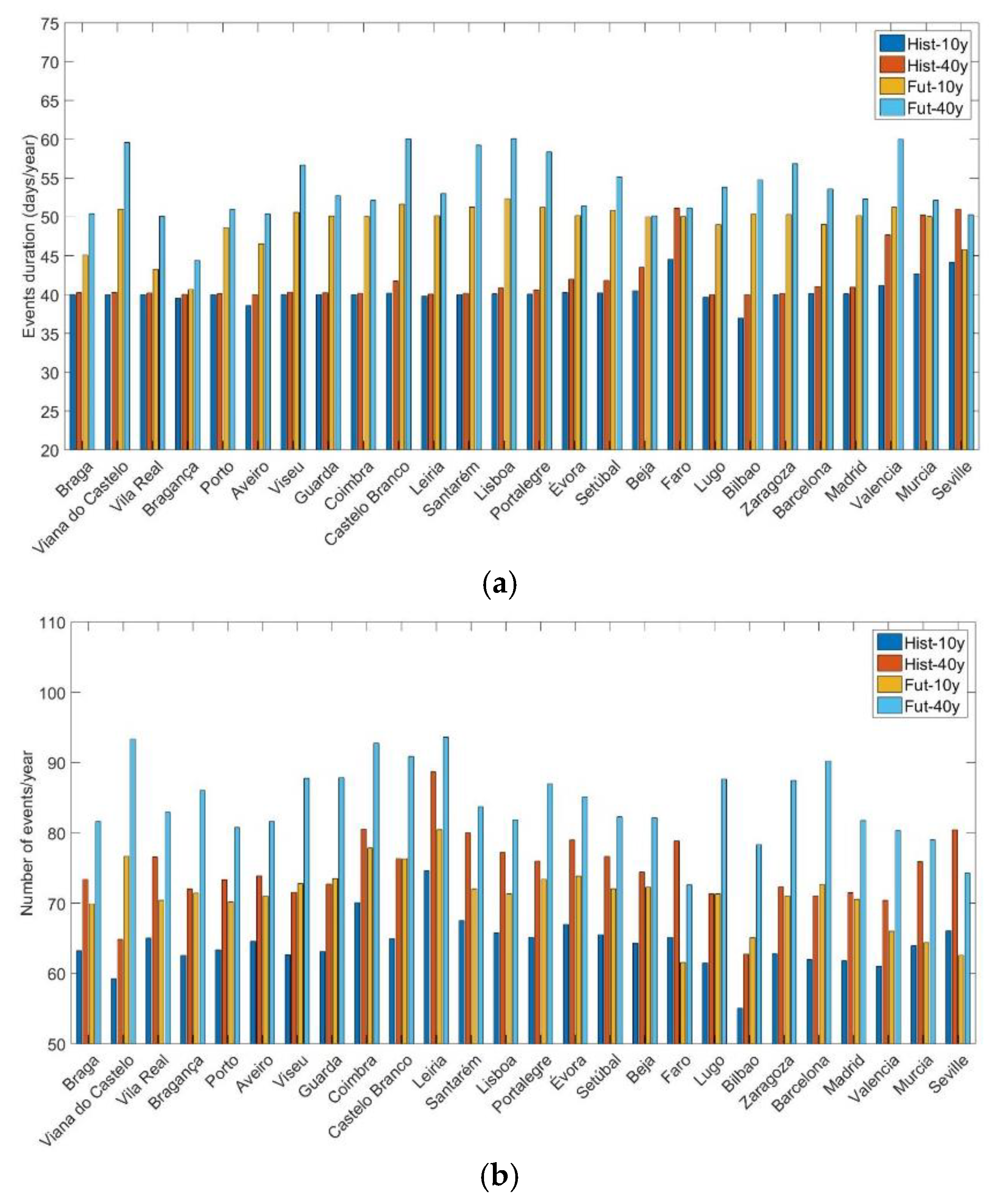
Figure 25.
Comparison of the (a) event duration (days/year) and (b) the number of events (year) in the historical (blue) and future (red) period for extreme events with a return period of 10 years (full line) and 40 years (dashed line) for wind shear (0–3 km).
Figure 25.
Comparison of the (a) event duration (days/year) and (b) the number of events (year) in the historical (blue) and future (red) period for extreme events with a return period of 10 years (full line) and 40 years (dashed line) for wind shear (0–3 km).
Figure 26.
Comparison of the (a) event duration (days/year) and (b) the number of events (year) in the historical (blue) and future (red) period for extreme events with a return period of 10 years (full line) and 40 years (dashed line) for helicity (0–6 km).
Figure 26.
Comparison of the (a) event duration (days/year) and (b) the number of events (year) in the historical (blue) and future (red) period for extreme events with a return period of 10 years (full line) and 40 years (dashed line) for helicity (0–6 km).
Table 1.
List of 26 cities considered in this study, along with their corresponding latitude and longitude (negative values of longitude refer to western hemisphere).
Table 1.
List of 26 cities considered in this study, along with their corresponding latitude and longitude (negative values of longitude refer to western hemisphere).
| Portugal |
|---|
| Cities | Latitude (°) | Longitude (°) |
|---|
| 1 | Braga | 41.54 | −8.43 |
| 2 | Viana do Castelo | 41.67 | −8.75 |
| 3 | Vila Real | 41.31 | −7.74 |
| 4 | Bragança | 41.80 | −6.78 |
| 5 | Porto | 41.17 | −8.58 |
| 6 | Aveiro | 10.75 | −8.67 |
| 7 | Viseu | 40.67 | −7.89 |
| 8 | Guarda | 40.65 | −7.25 |
| 9 | Coimbra | 40.16 | −8.40 |
| 10 | Castelo Branco | 39.80 | −7.47 |
| 11 | Leiria | 39.37 | −8.79 |
| 12 | Santarém | 39.24 | −8.71 |
| 13 | Lisboa | 38.50 | −9.08 |
| 14 | Portalegre | 39.28 | −7.45 |
| 15 | Évora | 38.57 | −7.92 |
| 16 | Setúbal | 38.56 | −8.90 |
| 17 | Beja | 38.00 | −7.85 |
| 18 | Faro | 37.08 | −7.83 |
| Spain |
| 19 | Lugo | 43.01 | −7.52 |
| 20 | Bilbao | 43.23 | −2.93 |
| 21 | Zaragoza | 41.63 | −0.92 |
| 22 | Barcelona | 41.33 | 2.08 |
| 23 | Madrid | 40.40 | −3.70 |
| 24 | Valencia | 39.50 | −0.33 |
| 25 | Murcia | 37.98 | −1.11 |
| 26 | Sevilla | 37.39 | −6.00 |
Table 2.
Reference values for S 0–6 and storm-relative helicity (SRH) 0–3 from [
31]. Values in each cell represent median/75th percentile/90th percentile. F represents the tornado category according to the Fujita scale.
Table 2.
Reference values for S 0–6 and storm-relative helicity (SRH) 0–3 from [
31]. Values in each cell represent median/75th percentile/90th percentile. F represents the tornado category according to the Fujita scale.
| Variable | Non-Supercell Storms | Supercell Storms Tornados F0 and F1 | Tornadic Supercells Tornados F2–F5 |
|---|
| S 0–6 (m s−1) | 10.8/15.7/22.0 | 19.1/22.1/25.8 | 18.4/21.8/29.0 |
| SRH 0–3 (m2 s−2) | 55/100/168 | 124/208/304 | 180/279/411 |
Table 3.
Reference values for SRH 0–3 from [
28] for different types of storms. Values in each cell represent median/75th percentile/90th percentile. F represents the tornado category according to the Fujita scale.
Table 3.
Reference values for SRH 0–3 from [
28] for different types of storms. Values in each cell represent median/75th percentile/90th percentile. F represents the tornado category according to the Fujita scale.
| Variable | Non-Supercell Storms | Non-Tornadic Supercells | Weakly Tornadic Storms F0–F1 | Significant Tornadic Supercells F2–F5 |
|---|
| S 0–6 (m s−1) | 7.8/11.0/14.3 | 22.3/27.3/31.1 | 22.8/26.8/31.1 | 24.5/29.2/31.8 |
| SRH 0–3 (m2 s−2) | - | 146/233/362 | 184/280/367.5 | 223/317/396 |
Table 4.
Reference values for SRH 0–3 from [
62] for each tornado category according to the Fujita scale.
Table 4.
Reference values for SRH 0–3 from [
62] for each tornado category according to the Fujita scale.
| Variable | F0 | F1 | F2 | F3 | F4 |
|---|
| SRH 0–3 (m2 s−2) | 66 | 140 | 196 | 226 | 249 |
Table 5.
Monthly and annual averaged wind speed near the surface for each city and the difference between the future and the historical climates. Significant differences (t-student 5%) are shown in red (positive) and blue (negative).
Table 5.
Monthly and annual averaged wind speed near the surface for each city and the difference between the future and the historical climates. Significant differences (t-student 5%) are shown in red (positive) and blue (negative).
| | | Months |
|---|
| CITIES | January | February | March | April | May | June | July | August | September | October | November | December | Year |
|---|
| Braga | MPI-hist | 7.05 | 6.63 | 5.66 | 5.20 | 4.28 | 3.69 | 3.74 | 3.77 | 4.07 | 4.78 | 5.76 | 6.53 | 5.09 |
| Differ. | −0.49 | −0.02 | −0.25 | −0.40 | −0.20 | −0.01 | 0.10 | −0.08 | −0.34 | −0.55 | 0.03 | −0.42 | −0.22 |
| Viana do Castelo | MPI-hist | 8.57 | 8.33 | 7.40 | 6.86 | 6.29 | 5.91 | 6.46 | 6.37 | 6.21 | 6.41 | 7.23 | 8.12 | 7.01 |
| Differ. | −0.62 | −0.08 | −0.48 | −0.17 | −0.10 | 0.46 | 0.26 | 0.26 | −0.05 | −0.62 | 0.01 | −0.44 | −0.13 |
| Vila Real | MPI-hist | 6.89 | 6.80 | 6.00 | 5.73 | 5.02 | 4.29 | 4.64 | 4.68 | 4.88 | 5.04 | 5.88 | 6.53 | 5.53 |
| Differ. | −0.44 | −0.22 | −0.45 | −0.39 | −0.26 | 0.23 | 0.03 | −0.10 | −0.17 | −0.13 | −0.10 | −0.63 | −0.22 |
| Bragança | MPI-hist | 5.96 | 6.01 | 5.67 | 5.55 | 5.43 | 4.80 | 5.01 | 5.15 | 5.10 | 5.07 | 5.51 | 5.65 | 5.41 |
| Differ. | −0.35 | −0.34 | −0.49 | −0.14 | −0.23 | 0.14 | 0.02 | −0.36 | −0.16 | −0.03 | −0.30 | −0.72 | −0.25 |
| Porto | MPI-hist | 7.96 | 7.44 | 6.05 | 5.49 | 4.57 | 3.89 | 4.12 | 4.04 | 4.27 | 4.82 | 6.03 | 7.34 | 5.50 |
| Differ. | −0.81 | −0.21 | −0.41 | −0.49 | −0.29 | 0.07 | −0.07 | −0.18 | −0.35 | −0.69 | −0.10 | −0.70 | −0.36 |
| Aveiro | MPI-hist | 9.34 | 8.91 | 7.59 | 7.09 | 6.08 | 5.25 | 5.53 | 5.53 | 5.66 | 6.24 | 7.44 | 8.79 | 6.94 |
| Differ. | −0.68 | −0.07 | −0.47 | −0.52 | −0.29 | 0.14 | −0.17 | −0.45 | −0.33 | −0.75 | −0.07 | −0.60 | −0.36 |
| Viseu | MPI-hist | 4.33 | 4.29 | 4.15 | 4.10 | 3.89 | 3.68 | 3.81 | 3.78 | 3.71 | 3.64 | 3.92 | 3.99 | 3.94 |
| Differ. | −0.25 | −0.15 | −0.33 | −0.16 | −0.03 | 0.17 | −0.01 | −0.17 | −0.14 | −0.15 | −0.19 | −0.26 | −0.14 |
| Guarda | MPI-hist | 6.26 | 6.02 | 5.68 | 5.03 | 4.20 | 3.78 | 3.73 | 3.79 | 4.34 | 5.34 | 6.10 | 6.00 | 5.02 |
| Differ. | 0.27 | 0.02 | −0.46 | −0.33 | −0.09 | −0.01 | 0.16 | −0.20 | −0.35 | −0.74 | −0.10 | 0.36 | −0.12 |
| Coimbra | MPI-hist | 6.58 | 6.15 | 5.48 | 5.05 | 4.34 | 3.87 | 3.98 | 4.01 | 4.28 | 5.02 | 6.05 | 6.50 | 5.10 |
| Differ. | −0.10 | −0.01 | −0.38 | −0.29 | 0.06 | 0.04 | −0.11 | −0.20 | −0.30 | −0.55 | −0.11 | −0.27 | −0.19 |
| Castelo Branco | MPI-hist | 6.33 | 6.07 | 5.57 | 5.32 | 4.74 | 4.72 | 5.03 | 5.11 | 5.07 | 5.23 | 5.78 | 6.21 | 5.43 |
| Differ. | −0.32 | −0.32 | −0.50 | −0.32 | 0.08 | 0.29 | 0.29 | −0.10 | −0.02 | 0.07 | −0.16 | −0.70 | −0.14 |
| Leiria | MPI-hist | 7.28 | 6.76 | 6.08 | 5.90 | 5.30 | 4.62 | 5.02 | 4.97 | 5.00 | 5.42 | 6.51 | 7.17 | 5.83 |
| Differ. | −0.60 | −0.09 | −0.41 | −0.30 | −0.09 | 0.23 | −0.23 | −0.16 | −0.12 | −0.28 | −0.15 | −0.77 | −0.25 |
| Santarém | MPI-hist | 6.22 | 5.88 | 5.45 | 5.27 | 4.61 | 4.46 | 4.76 | 5.01 | 4.96 | 5.18 | 5.72 | 5.99 | 5.29 |
| Differ. | −0.23 | −0.21 | −0.39 | −0.34 | 0.12 | 0.20 | 0.01 | −0.26 | −0.01 | −0.03 | −0.06 | −0.58 | −0.15 |
| Lisboa | MPI-hist | 6.43 | 6.35 | 6.05 | 6.15 | 5.92 | 6.20 | 6.87 | 6.87 | 6.14 | 5.77 | 5.99 | 6.17 | 6.24 |
| Differ. | −0.11 | −0.33 | −0.25 | −0.14 | 0.28 | 0.76 | 0.39 | 0.20 | 0.46 | 0.28 | −0.06 | −0.49 | 0.08 |
| Portalegre | MPI-hist | 6.86 | 6.74 | 6.25 | 6.18 | 5.73 | 6.03 | 6.45 | 6.47 | 5.97 | 5.73 | 6.17 | 6.48 | 6.25 |
| Differ. | −0.29 | −0.38 | −0.30 | −0.17 | 0.29 | 0.50 | 0.54 | 0.05 | 0.32 | 0.31 | −0.11 | −0.56 | 0.02 |
| Évora | MPI-hist | 7.15 | 7.08 | 6.55 | 6.81 | 6.43 | 6.93 | 7.49 | 7.40 | 6.57 | 6.19 | 6.48 | 6.80 | 6.82 |
| Differ. | −0.17 | −0.19 | 0.01 | −0.17 | 0.39 | 0.71 | 0.50 | 0.18 | 0.64 | 0.29 | 0.07 | −0.43 | 0.15 |
| Setúbal | MPI-hist | 6.76 | 6.73 | 6.38 | 6.56 | 6.32 | 6.79 | 7.40 | 7.34 | 6.49 | 6.04 | 6.21 | 6.44 | 6.62 |
| Differ. | −0.13 | −0.26 | −0.09 | −0.11 | 0.37 | 0.81 | 0.49 | 0.25 | 0.59 | 0.29 | 0.02 | −0.39 | 0.15 |
| Beja | MPI-hist | 7.23 | 7.11 | 6.50 | 6.95 | 6.40 | 6.76 | 7.00 | 6.97 | 6.16 | 5.99 | 6.37 | 6.95 | 6.70 |
| Differ. | −0.38 | −0.28 | 0.00 | −0.40 | 0.23 | 0.55 | 0.53 | 0.13 | 0.70 | 0.07 | 0.05 | −0.72 | 0.04 |
| Faro | MPI-hist | 6.45 | 6.28 | 5.60 | 5.69 | 4.67 | 4.18 | 3.80 | 4.03 | 4.51 | 5.48 | 6.22 | 6.29 | 5.26 |
| Differ. | −0.11 | −0.42 | 0.09 | −0.60 | −0.22 | −0.24 | −0.43 | −0.78 | −0.32 | −0.88 | −0.89 | −0.71 | −0.46 |
| Lugo | MPI-hist | 6.60 | 6.46 | 6.07 | 5.64 | 5.18 | 5.25 | 4.96 | 5.04 | 5.36 | 5.65 | 6.30 | 6.47 | 5.74 |
| Differ. | 0.13 | 0.27 | 0.07 | 0.00 | 0.09 | −0.01 | 0.77 | 0.61 | −0.02 | −0.21 | −0.10 | 0.18 | 0.15 |
| Bilbao | MPI-hist | 6.74 | 6.48 | 5.58 | 4.95 | 4.24 | 3.58 | 3.35 | 3.51 | 3.87 | 4.86 | 5.86 | 6.50 | 4.95 |
| Differ. | −0.25 | −0.31 | −0.33 | −0.49 | −0.34 | −0.26 | −0.19 | −0.40 | −0.19 | −0.57 | −0.33 | −0.07 | −0.31 |
| Zaragoza | MPI-hist | 7.12 | 6.95 | 6.14 | 6.41 | 5.27 | 4.80 | 4.57 | 4.66 | 4.90 | 5.56 | 6.36 | 7.15 | 5.82 |
| Differ. | −0.53 | −0.30 | −0.20 | −0.67 | −0.08 | −0.28 | −0.13 | −0.31 | −0.16 | −0.33 | −0.64 | −1.13 | −0.40 |
| Barcelona | MPI-hist | 5.40 | 5.18 | 4.93 | 4.92 | 4.39 | 4.14 | 3.96 | 4.17 | 4.48 | 4.92 | 5.29 | 5.38 | 4.76 |
| Differ. | −0.17 | −0.28 | −0.12 | −0.28 | 0.03 | −0.21 | −0.05 | −0.15 | −0.16 | −0.15 | −0.37 | −0.59 | −0.21 |
| Madrid | MPI-hist | 5.97 | 5.75 | 5.38 | 5.09 | 4.67 | 4.44 | 4.52 | 4.52 | 4.72 | 4.69 | 5.38 | 5.61 | 5.06 |
| Differ. | −0.12 | −0.12 | −0.17 | −0.10 | 0.09 | −0.06 | 0.14 | −0.30 | −0.28 | 0.19 | −0.27 | −0.40 | −0.12 |
| Valencia | MPI-hist | 5.67 | 5.38 | 5.27 | 5.14 | 4.47 | 4.39 | 4.11 | 4.32 | 4.66 | 5.26 | 5.91 | 5.90 | 5.04 |
| Differ. | 0.00 | −0.21 | −0.11 | −0.31 | 0.12 | −0.08 | 0.09 | −0.27 | −0.04 | −0.09 | −0.39 | −0.34 | −0.14 |
| Murcia | MPI-hist | 4.38 | 4.34 | 4.06 | 4.42 | 3.84 | 3.33 | 3.15 | 3.22 | 3.24 | 3.52 | 3.89 | 4.06 | 3.78 |
| Differ. | −0.17 | −0.19 | −0.08 | −0.45 | −0.18 | −0.12 | 0.04 | −0.14 | −0.08 | −0.26 | −0.25 | −0.39 | −0.19 |
| Sevilla | MPI-hist | 5.81 | 5.60 | 5.02 | 5.16 | 3.98 | 3.59 | 3.08 | 3.27 | 3.63 | 4.80 | 5.58 | 5.83 | 4.61 |
| Differ. | −0.06 | −0.25 | 0.21 | −0.66 | −0.19 | −0.24 | −0.18 | −0.54 | −0.20 | −0.81 | −0.64 | −0.72 | −0.36 |
Table 6.
Monthly and annual averaged wind speed at 850 hPa for each city and the difference between the future and the historical climates. Significant differences (t-student 5%) are shown in red (positive) and blue (negative).
Table 6.
Monthly and annual averaged wind speed at 850 hPa for each city and the difference between the future and the historical climates. Significant differences (t-student 5%) are shown in red (positive) and blue (negative).
| | | Months |
|---|
| CITIES | January | February | March | April | May | June | July | August | September | October | November | December | Year |
|---|
| Braga | MPI-hist | 12.69 | 12.01 | 10.70 | 9.38 | 7.63 | 6.61 | 6.41 | 6.44 | 7.33 | 9.29 | 10.83 | 12.09 | 9.27 |
| Differ. | 0.06 | 0.45 | −0.04 | −0.12 | 0.00 | −0.42 | −0.53 | −0.96 | −0.88 | −1.60 | 0.12 | 0.14 | −0.32 |
| Viana do Castelo | MPI-hist | 12.99 | 12.27 | 10.93 | 9.44 | 7.64 | 6.50 | 6.03 | 6.19 | 7.31 | 9.43 | 11.13 | 12.49 | 9.35 |
| Differ. | 0.01 | 0.43 | −0.17 | −0.13 | −0.10 | −0.53 | −0.47 | −1.04 | −1.01 | −1.65 | 0.14 | 0.09 | −0.38 |
| Vila Real | MPI-hist | 12.59 | 11.95 | 10.70 | 9.59 | 7.93 | 7.09 | 7.29 | 7.12 | 7.63 | 9.33 | 10.66 | 11.89 | 9.47 |
| Differ. | 0.08 | 0.48 | 0.18 | 0.08 | 0.18 | −0.23 | −0.48 | −0.77 | −0.61 | −1.39 | 0.16 | 0.17 | −0.18 |
| Bragança | MPI-hist | 11.89 | 11.16 | 10.06 | 8.83 | 7.21 | 6.13 | 5.78 | 5.97 | 6.86 | 8.57 | 9.99 | 11.08 | 8.62 |
| Differ. | −0.45 | 0.11 | −0.21 | −0.01 | −0.06 | −0.67 | −0.48 | −1.10 | −0.75 | −1.16 | −0.08 | −0.18 | −0.42 |
| Porto | MPI-hist | 12.60 | 12.00 | 10.77 | 9.46 | 7.73 | 6.61 | 6.62 | 6.54 | 7.39 | 9.20 | 10.71 | 11.93 | 9.29 |
| Differ. | 0.21 | 0.45 | −0.02 | −0.19 | 0.04 | −0.26 | −0.55 | −0.89 | −0.86 | −1.51 | 0.14 | 0.24 | −0.27 |
| Aveiro | MPI-hist | 12.95 | 12.32 | 10.98 | 9.71 | 7.94 | 6.80 | 7.03 | 6.77 | 7.56 | 9.28 | 10.90 | 12.11 | 9.52 |
| Differ. | 0.26 | 0.42 | 0.10 | −0.26 | 0.11 | −0.07 | −0.54 | −0.64 | −0.85 | −1.43 | 0.14 | 0.18 | −0.22 |
| Viseu | MPI-hist | 10.51 | 9.99 | 8.99 | 7.97 | 6.70 | 5.80 | 5.50 | 5.59 | 6.25 | 7.76 | 9.00 | 9.70 | 7.80 |
| Differ. | −0.12 | −0.26 | −0.23 | −0.10 | −0.09 | −0.41 | −0.32 | −0.78 | −0.50 | −1.16 | −0.25 | −0.14 | −0.36 |
| Guarda | MPI-hist | 10.25 | 9.88 | 9.10 | 8.26 | 7.11 | 5.95 | 5.69 | 5.77 | 6.35 | 7.86 | 9.07 | 9.50 | 7.89 |
| Differ. | −0.10 | −0.32 | −0.27 | 0.11 | −0.19 | −0.49 | −0.31 | −0.91 | −0.42 | −1.14 | −0.44 | −0.30 | −0.40 |
| Coimbra | MPI-hist | 10.10 | 9.75 | 8.82 | 8.08 | 6.87 | 5.79 | 5.41 | 5.48 | 6.17 | 7.53 | 8.75 | 9.39 | 7.67 |
| Differ. | 0.01 | −0.32 | −0.24 | −0.28 | −0.21 | −0.40 | −0.34 | −0.78 | −0.57 | −1.12 | −0.37 | −0.25 | −0.41 |
| Castelo Branco | MPI-hist | 9.84 | 9.57 | 8.65 | 8.05 | 6.74 | 5.53 | 4.97 | 5.17 | 5.94 | 7.50 | 8.62 | 9.16 | 7.47 |
| Differ. | 0.06 | −0.17 | −0.12 | −0.36 | −0.36 | −0.60 | −0.28 | −0.76 | −0.50 | −1.21 | −0.33 | −0.12 | −0.40 |
| Leiria | MPI-hist | 10.17 | 9.85 | 8.96 | 8.33 | 7.08 | 5.88 | 5.44 | 5.53 | 6.19 | 7.65 | 8.85 | 9.49 | 7.77 |
| Differ. | 0.04 | −0.36 | −0.35 | −0.45 | −0.33 | −0.39 | −0.40 | −0.78 | −0.52 | −1.13 | −0.35 | −0.31 | −0.45 |
| Santarém | MPI-hist | 9.87 | 9.62 | 8.73 | 8.19 | 6.89 | 5.69 | 5.11 | 5.23 | 6.01 | 7.53 | 8.74 | 9.25 | 7.56 |
| Differ. | 0.09 | −0.31 | −0.25 | −0.54 | −0.40 | −0.43 | −0.17 | −0.57 | −0.46 | −1.19 | −0.42 | −0.31 | −0.41 |
| Lisboa | MPI-hist | 10.01 | 9.88 | 8.88 | 8.45 | 7.13 | 5.79 | 5.28 | 5.33 | 6.08 | 7.63 | 8.88 | 9.42 | 7.72 |
| Differ. | 0.11 | −0.47 | −0.34 | −0.66 | −0.47 | −0.36 | −0.07 | −0.47 | −0.36 | −1.22 | −0.49 | −0.50 | −0.44 |
| Portalegre | MPI-hist | 10.32 | 10.07 | 8.97 | 8.58 | 7.13 | 5.63 | 5.13 | 5.18 | 5.99 | 7.70 | 8.93 | 9.47 | 7.75 |
| Differ. | −0.03 | −0.24 | −0.17 | −0.62 | −0.58 | −0.61 | −0.15 | −0.51 | −0.45 | −1.37 | −0.45 | −0.30 | −0.46 |
| Évora | MPI-hist | 10.53 | 10.38 | 9.02 | 8.81 | 7.17 | 5.43 | 5.02 | 5.09 | 5.88 | 7.60 | 9.04 | 9.59 | 7.78 |
| Differ. | −0.08 | −0.46 | −0.18 | −0.84 | −0.69 | −0.43 | −0.14 | −0.49 | −0.52 | −1.38 | −0.55 | −0.53 | −0.52 |
| Setúbal | MPI-hist | 10.19 | 10.11 | 8.95 | 8.61 | 7.20 | 5.68 | 5.17 | 5.25 | 5.99 | 7.61 | 8.97 | 9.47 | 7.75 |
| Differ. | 0.06 | −0.50 | −0.29 | −0.75 | −0.55 | −0.37 | −0.08 | −0.51 | −0.38 | −1.29 | −0.51 | −0.54 | −0.48 |
| Beja | MPI-hist | 10.80 | 10.59 | 9.08 | 9.01 | 7.21 | 5.27 | 5.14 | 5.02 | 5.79 | 7.47 | 9.05 | 9.70 | 7.83 |
| Differ. | −0.20 | −0.53 | −0.15 | −0.95 | −0.74 | −0.32 | −0.32 | −0.44 | −0.53 | −1.34 | −0.56 | −0.74 | −0.57 |
| Faro | MPI-hist | 9.68 | 9.29 | 7.94 | 8.18 | 6.49 | 5.58 | 4.78 | 5.12 | 5.83 | 7.38 | 8.39 | 9.06 | 7.30 |
| Differ. | −0.17 | −0.47 | 0.35 | −0.76 | −0.38 | −0.23 | −0.06 | −0.99 | −0.43 | −1.40 | −0.84 | −0.86 | −0.52 |
| Lugo | MPI-hist | 13.60 | 13.00 | 11.56 | 9.86 | 8.11 | 6.97 | 6.55 | 6.78 | 7.92 | 10.13 | 11.79 | 13.15 | 9.94 |
| Differ. | −0.10 | 0.46 | −0.03 | 0.20 | 0.00 | −0.61 | −0.74 | −1.39 | −1.04 | −1.74 | 0.13 | 0.11 | −0.40 |
| Bilbao | MPI-hist | 12.17 | 11.40 | 10.30 | 8.80 | 7.72 | 7.01 | 7.51 | 7.39 | 7.82 | 9.07 | 10.31 | 11.63 | 9.25 |
| Differ. | −0.34 | 0.62 | 0.20 | 0.83 | 0.52 | 0.12 | −0.26 | −0.93 | −0.57 | −1.04 | 0.00 | 0.03 | −0.08 |
| Zaragoza | MPI-hist | 12.47 | 11.81 | 10.27 | 9.81 | 7.99 | 6.30 | 5.83 | 6.22 | 6.93 | 8.73 | 10.43 | 12.00 | 9.05 |
| Differ. | −0.92 | 0.14 | −0.18 | −0.62 | −0.52 | −0.69 | −0.40 | −1.40 | −0.77 | −0.96 | −0.13 | −0.92 | −0.62 |
| Barcelona | MPI-hist | 10.74 | 10.01 | 8.68 | 7.98 | 6.51 | 5.35 | 4.78 | 5.22 | 6.01 | 7.51 | 8.97 | 10.61 | 7.69 |
| Differ. | −0.47 | 0.44 | 0.19 | −0.28 | −0.28 | −0.64 | −0.47 | −1.33 | −1.01 | −1.06 | −0.02 | −0.82 | −0.49 |
| Madrid | MPI-hist | 10.70 | 10.36 | 9.21 | 8.33 | 7.11 | 5.56 | 5.47 | 5.53 | 6.37 | 7.72 | 9.14 | 9.76 | 7.93 |
| Differ. | −0.32 | −0.12 | −0.20 | 0.12 | −0.27 | −0.40 | −0.37 | −0.73 | −0.83 | −0.94 | −0.54 | −0.30 | −0.41 |
| Valencia | MPI-hist | 10.74 | 10.09 | 8.49 | 8.17 | 6.20 | 5.25 | 4.57 | 4.72 | 5.57 | 7.13 | 8.60 | 10.20 | 7.46 |
| Differ. | −0.54 | 0.22 | 0.14 | −0.74 | −0.36 | −0.60 | 0.04 | −0.77 | −0.85 | −1.31 | 0.02 | −0.97 | −0.48 |
| Murcia | MPI-hist | 10.24 | 9.67 | 8.19 | 7.92 | 6.11 | 5.10 | 4.45 | 4.69 | 5.44 | 7.07 | 8.36 | 9.46 | 7.21 |
| Differ. | −0.42 | −0.18 | 0.17 | −0.73 | −0.38 | −0.40 | 0.05 | −0.57 | −0.60 | −1.27 | −0.33 | −0.94 | −0.47 |
| Sevilla | MPI-hist | 9.65 | 9.08 | 7.71 | 7.80 | 6.12 | 5.41 | 4.62 | 4.91 | 5.64 | 7.21 | 8.26 | 8.84 | 7.09 |
| Differ. | −0.39 | −0.32 | 0.40 | −0.69 | −0.42 | −0.39 | 0.20 | −0.68 | −0.37 | −1.26 | −0.68 | −0.77 | −0.45 |
Table 7.
Monthly and annual averaged wind speed at 300 hPa for each city and the difference between the future and the historical climates. Significant differences (t-student 5%) are shown in red (positive) and blue (negative).
Table 7.
Monthly and annual averaged wind speed at 300 hPa for each city and the difference between the future and the historical climates. Significant differences (t-student 5%) are shown in red (positive) and blue (negative).
| | | Months |
|---|
| CITIES | January | February | March | April | May | June | July | August | September | October | November | December | Year |
|---|
| Braga | MPI-hist | 28.21 | 27.46 | 24.36 | 24.07 | 21.47 | 18.23 | 19.51 | 18.68 | 20.19 | 23.37 | 24.76 | 26.45 | 23.04 |
| Differ. | 2.83 | 3.15 | 2.76 | 1.57 | 2.14 | 0.16 | −3.09 | −3.24 | −2.31 | −2.06 | 3.18 | 1.76 | 0.55 |
| Viana do Castelo | MPI-hist | 28.20 | 27.42 | 24.30 | 24.07 | 21.47 | 18.15 | 19.31 | 18.62 | 20.20 | 23.48 | 24.83 | 26.49 | 23.03 |
| Differ. | 2.88 | 3.16 | 2.74 | 1.40 | 1.96 | 0.15 | −2.96 | −3.29 | −2.41 | −2.15 | 3.18 | 1.85 | 0.52 |
| Vila Real | MPI-hist | 28.17 | 27.43 | 24.36 | 24.07 | 21.48 | 18.39 | 19.90 | 18.91 | 20.30 | 23.30 | 24.68 | 26.33 | 23.09 |
| Differ. | 2.92 | 3.40 | 3.02 | 1.96 | 2.47 | 0.24 | −3.18 | −3.09 | −2.27 | −1.67 | 3.37 | 1.87 | 0.73 |
| Bragança | MPI-hist | 28.01 | 27.29 | 24.05 | 23.54 | 21.07 | 18.02 | 19.44 | 18.73 | 20.07 | 23.16 | 24.63 | 26.32 | 22.84 |
| Differ. | 2.54 | 3.07 | 2.50 | 1.78 | 2.23 | 0.33 | −3.36 | −3.44 | −2.30 | −1.92 | 2.93 | 1.46 | 0.46 |
| Porto | MPI-hist | 27.95 | 27.35 | 24.43 | 24.34 | 21.61 | 18.39 | 19.58 | 18.62 | 20.13 | 23.28 | 24.59 | 26.16 | 23.02 |
| Differ. | 2.91 | 3.28 | 2.90 | 1.58 | 2.28 | 0.01 | −3.09 | −3.11 | −2.37 | −2.06 | 3.15 | 1.82 | 0.59 |
| Aveiro | MPI-hist | 27.70 | 27.27 | 24.42 | 24.62 | 21.82 | 18.51 | 19.68 | 18.57 | 20.01 | 23.05 | 24.29 | 25.71 | 22.95 |
| Differ. | 3.02 | 3.28 | 3.12 | 1.56 | 2.45 | −0.05 | −3.07 | −2.86 | −2.44 | −1.85 | 3.16 | 1.89 | 0.67 |
| Viseu | MPI-hist | 28.29 | 27.81 | 24.63 | 24.70 | 21.57 | 18.07 | 19.23 | 18.13 | 19.56 | 22.92 | 24.52 | 26.03 | 22.93 |
| Differ. | 2.53 | 2.77 | 2.70 | 1.09 | 2.09 | −0.16 | −3.43 | −2.97 | −2.44 | −1.94 | 2.88 | 1.37 | 0.36 |
| Guarda | MPI-hist | 28.00 | 27.41 | 24.18 | 24.09 | 21.09 | 17.90 | 19.06 | 18.00 | 19.27 | 22.48 | 24.04 | 25.71 | 22.58 |
| Differ. | 2.36 | 2.67 | 2.73 | 1.29 | 2.23 | −0.12 | −3.52 | −2.93 | −2.35 | −1.67 | 2.85 | 1.18 | 0.38 |
| Coimbra | MPI-hist | 28.09 | 27.64 | 24.55 | 24.73 | 21.45 | 17.88 | 18.83 | 17.63 | 19.08 | 22.45 | 24.08 | 25.62 | 22.65 |
| Differ. | 2.29 | 2.45 | 2.51 | 0.81 | 1.94 | −0.33 | −3.33 | −2.72 | −2.50 | −1.98 | 2.69 | 1.08 | 0.23 |
| Castelo Branco | MPI-hist | 27.97 | 27.66 | 24.55 | 24.85 | 21.56 | 18.05 | 18.84 | 17.66 | 18.98 | 22.09 | 23.72 | 25.32 | 22.58 |
| Differ. | 2.17 | 2.33 | 2.54 | 0.96 | 2.03 | −0.35 | −3.19 | −2.54 | −2.55 | −1.55 | 2.76 | 1.02 | 0.29 |
| Leiria | MPI-hist | 27.98 | 27.66 | 24.65 | 24.98 | 21.59 | 17.94 | 18.71 | 17.48 | 18.96 | 22.34 | 23.98 | 25.40 | 22.61 |
| Differ. | 2.27 | 2.34 | 2.48 | 0.69 | 1.90 | −0.47 | −3.10 | −2.52 | −2.56 | −1.93 | 2.53 | 1.08 | 0.21 |
| Santarém | MPI-hist | 27.84 | 27.65 | 24.69 | 25.24 | 21.80 | 18.01 | 18.60 | 17.35 | 18.79 | 22.01 | 23.70 | 25.09 | 22.54 |
| Differ. | 2.13 | 2.20 | 2.39 | 0.63 | 1.82 | −0.42 | −2.92 | −2.30 | −2.60 | −1.71 | 2.41 | 0.90 | 0.20 |
| Lisboa | MPI-hist | 27.67 | 27.70 | 24.81 | 25.68 | 22.20 | 18.19 | 18.50 | 17.26 | 18.67 | 21.84 | 23.60 | 24.85 | 22.55 |
| Differ. | 2.12 | 2.13 | 2.38 | 0.56 | 1.60 | −0.37 | −2.59 | −2.00 | −2.58 | −1.55 | 2.14 | 0.77 | 0.20 |
| Portalegre | MPI-hist | 27.85 | 27.71 | 24.69 | 25.18 | 21.99 | 18.28 | 18.72 | 17.63 | 18.88 | 21.85 | 23.61 | 25.08 | 22.60 |
| Differ. | 2.07 | 2.23 | 2.47 | 0.99 | 1.95 | −0.31 | −2.83 | −2.37 | −2.52 | −1.24 | 2.62 | 0.90 | 0.32 |
| Évora | MPI-hist | 27.82 | 27.93 | 25.00 | 25.95 | 22.74 | 18.57 | 18.68 | 17.46 | 18.66 | 21.68 | 23.60 | 24.84 | 22.72 |
| Differ. | 1.95 | 2.14 | 2.35 | 0.86 | 1.54 | −0.28 | −2.51 | −2.00 | −2.48 | −1.13 | 2.31 | 0.72 | 0.28 |
| Setúbal | MPI-hist | 27.68 | 27.77 | 24.87 | 25.84 | 22.43 | 18.32 | 18.56 | 17.28 | 18.57 | 21.75 | 23.55 | 24.81 | 22.59 |
| Differ. | 2.06 | 2.10 | 2.36 | 0.62 | 1.53 | −0.32 | −2.56 | −1.95 | −2.49 | −1.41 | 2.13 | 0.69 | 0.22 |
| Beja | MPI-hist | 27.90 | 28.24 | 25.30 | 26.52 | 23.41 | 18.76 | 18.72 | 17.40 | 18.52 | 21.53 | 23.68 | 24.79 | 22.87 |
| Differ. | 1.90 | 2.04 | 2.25 | 0.86 | 1.27 | −0.02 | −2.34 | −1.75 | −2.35 | −0.95 | 2.07 | 0.56 | 0.28 |
| Faro | MPI-hist | 25.92 | 25.54 | 22.85 | 24.38 | 20.09 | 16.15 | 15.34 | 14.81 | 16.20 | 20.54 | 22.88 | 23.67 | 20.67 |
| Differ. | 2.40 | 2.72 | 2.33 | 0.06 | 0.57 | −1.53 | −1.81 | −1.86 | −1.75 | −2.61 | 0.74 | 0.06 | −0.07 |
| Lugo | MPI-hist | 28.46 | 27.34 | 24.11 | 23.14 | 21.24 | 18.51 | 19.62 | 19.61 | 20.79 | 24.09 | 25.21 | 27.11 | 23.25 |
| Differ. | 2.62 | 3.34 | 2.57 | 2.09 | 1.78 | 0.32 | −2.52 | −3.86 | −2.18 | −2.23 | 3.41 | 2.04 | 0.59 |
| Bilbao | MPI-hist | 28.06 | 27.20 | 23.83 | 22.25 | 20.51 | 18.97 | 20.63 | 20.53 | 21.55 | 23.67 | 25.14 | 26.84 | 23.25 |
| Differ. | 2.43 | 3.69 | 2.81 | 3.46 | 3.40 | 0.89 | −2.85 | −3.92 | −2.46 | −1.38 | 2.57 | 2.20 | 0.88 |
| Zaragoza | MPI-hist | 28.96 | 27.62 | 24.35 | 23.59 | 21.21 | 18.02 | 17.38 | 18.25 | 19.81 | 23.74 | 25.72 | 27.67 | 23.01 |
| Differ. | 1.81 | 3.35 | 2.89 | 1.94 | 1.46 | −1.25 | −2.00 | −4.05 | −2.70 | −2.19 | 3.00 | 1.36 | 0.28 |
| Barcelona | MPI-hist | 28.74 | 27.28 | 24.44 | 22.80 | 20.70 | 17.94 | 17.16 | 18.08 | 19.90 | 23.42 | 25.65 | 27.12 | 22.75 |
| Differ. | 1.78 | 3.50 | 3.09 | 2.18 | 1.89 | −0.76 | −1.93 | −3.80 | −2.89 | −2.25 | 2.53 | 1.71 | 0.40 |
| Madrid | MPI-hist | 27.97 | 27.59 | 24.44 | 23.94 | 21.40 | 18.48 | 19.38 | 18.59 | 19.72 | 21.91 | 23.72 | 25.25 | 22.67 |
| Differ. | 1.88 | 2.56 | 2.70 | 2.20 | 2.75 | 0.26 | −3.67 | −3.01 | −3.09 | −0.85 | 2.70 | 1.24 | 0.46 |
| Valencia | MPI-hist | 28.36 | 27.00 | 23.99 | 23.30 | 20.44 | 17.19 | 16.65 | 16.62 | 18.35 | 21.74 | 24.53 | 25.38 | 21.94 |
| Differ. | 1.70 | 3.22 | 2.77 | 1.93 | 2.13 | −0.99 | −2.57 | −2.82 | −2.48 | −1.75 | 1.98 | 1.32 | 0.35 |
| Murcia | MPI-hist | 27.92 | 26.89 | 24.08 | 24.17 | 20.66 | 17.15 | 16.84 | 16.03 | 17.60 | 21.06 | 23.83 | 24.38 | 21.69 |
| Differ. | 1.47 | 2.97 | 2.83 | 1.44 | 1.89 | −1.04 | −2.50 | −1.64 | −2.14 | −1.77 | 1.79 | 0.88 | 0.33 |
| Sevilla | MPI-hist | 26.49 | 25.84 | 22.98 | 24.26 | 20.19 | 16.52 | 15.70 | 15.07 | 16.40 | 20.51 | 23.06 | 23.88 | 20.88 |
| Differ. | 2.04 | 2.77 | 2.46 | 0.46 | 0.90 | −1.61 | −2.11 | −1.81 | −1.70 | −2.37 | 1.05 | 0.13 | 0.00 |
Table 8.
Monthly and annual averaged wind shear 0–6 km for each city and the difference between the future and the historical climates. Significant differences (t-student 5%) are shown in red (positive) and blue (negative).
Table 8.
Monthly and annual averaged wind shear 0–6 km for each city and the difference between the future and the historical climates. Significant differences (t-student 5%) are shown in red (positive) and blue (negative).
| | | Months |
|---|
| CITIES | January | February | March | April | May | June | July | August | September | October | November | December | Year |
|---|
| Braga | MPI-hist | 17.05 | 16.73 | 15.42 | 14.83 | 13.51 | 12.27 | 13.71 | 12.74 | 12.56 | 14.16 | 14.82 | 15.98 | 14.47 |
| Differ. | 1.41 | 1.34 | 0.81 | 1.03 | 1.60 | 0.99 | −1.10 | −1.22 | −0.98 | −1.75 | 1.35 | 0.64 | 0.33 |
| Viana do Castelo | MPI-hist | 15.97 | 15.41 | 14.34 | 13.84 | 12.70 | 12.73 | 14.01 | 12.94 | 12.58 | 13.30 | 13.66 | 15.00 | 13.87 |
| Differ. | 1.34 | 1.44 | 1.03 | 0.91 | 1.64 | 1.01 | −0.25 | −0.37 | −0.46 | −1.46 | 1.52 | 0.65 | 0.58 |
| Vila Real | MPI-hist | 17.31 | 16.73 | 15.59 | 15.15 | 13.43 | 12.72 | 13.78 | 12.72 | 12.76 | 14.29 | 15.06 | 15.98 | 14.62 |
| Differ. | 1.58 | 1.66 | 0.99 | 0.73 | 1.75 | 0.50 | −1.09 | −1.07 | −0.94 | −1.66 | 1.37 | 1.13 | 0.40 |
| Bragança | MPI-hist | 18.98 | 18.55 | 16.40 | 15.54 | 13.77 | 12.47 | 12.86 | 12.29 | 13.06 | 15.22 | 16.49 | 17.83 | 15.27 |
| Differ. | 1.08 | 1.30 | 0.95 | 0.95 | 1.14 | −0.10 | −0.90 | −1.57 | −1.53 | −1.87 | 1.11 | 0.87 | 0.11 |
| Porto | MPI-hist | 16.11 | 15.86 | 14.88 | 14.53 | 13.20 | 12.24 | 13.41 | 12.35 | 12.41 | 13.86 | 14.33 | 15.12 | 14.02 |
| Differ. | 1.84 | 1.65 | 1.28 | 1.06 | 1.86 | 0.64 | −1.11 | −1.18 | −1.02 | −1.60 | 1.53 | 1.02 | 0.49 |
| Aveiro | MPI-hist | 14.90 | 14.56 | 14.08 | 13.74 | 12.55 | 12.48 | 13.68 | 12.22 | 11.93 | 12.74 | 13.19 | 13.80 | 13.32 |
| Differ. | 1.36 | 1.08 | 0.91 | 0.93 | 2.12 | 0.65 | −0.64 | −0.31 | −0.77 | −1.16 | 1.03 | 0.41 | 0.46 |
| Viseu | MPI-hist | 18.30 | 17.72 | 16.20 | 15.87 | 14.03 | 13.30 | 14.51 | 13.18 | 13.12 | 14.53 | 15.41 | 16.85 | 15.24 |
| Differ. | 1.58 | 1.93 | 1.53 | 0.79 | 2.00 | 0.64 | −1.02 | −0.74 | −1.26 | −1.61 | 1.67 | 1.25 | 0.55 |
| Guarda | MPI-hist | 17.81 | 17.06 | 15.91 | 15.52 | 13.83 | 13.12 | 14.70 | 13.37 | 12.99 | 13.74 | 14.77 | 16.06 | 14.90 |
| Differ. | 0.73 | 1.67 | 0.92 | 0.99 | 2.11 | 0.89 | −0.99 | −0.58 | −1.31 | −1.05 | 1.33 | 0.63 | 0.44 |
| Coimbra | MPI-hist | 16.75 | 16.37 | 15.72 | 15.61 | 14.28 | 13.63 | 15.46 | 14.12 | 13.28 | 13.68 | 14.11 | 15.11 | 14.84 |
| Differ. | 1.37 | 1.71 | 1.25 | 1.08 | 2.39 | 0.87 | −1.30 | −0.55 | −1.04 | −1.14 | 1.37 | 0.78 | 0.56 |
| Castelo Branco | MPI-hist | 16.83 | 16.46 | 15.81 | 15.72 | 14.17 | 14.19 | 16.05 | 14.61 | 13.70 | 14.15 | 14.40 | 15.11 | 15.10 |
| Differ. | 1.65 | 1.80 | 1.65 | 1.19 | 2.39 | 1.01 | −0.65 | 0.04 | −0.96 | −0.98 | 1.74 | 1.64 | 0.87 |
| Leiria | MPI-hist | 16.03 | 15.73 | 15.19 | 15.19 | 13.89 | 13.55 | 15.52 | 14.07 | 12.89 | 13.26 | 13.59 | 14.50 | 14.45 |
| Differ. | 1.62 | 1.48 | 1.25 | 0.93 | 2.47 | 0.94 | −1.18 | −0.17 | −0.77 | −1.19 | 1.03 | 0.60 | 0.58 |
| Santarém | MPI-hist | 16.19 | 15.90 | 15.50 | 15.44 | 13.98 | 13.81 | 15.94 | 14.52 | 13.32 | 13.64 | 13.86 | 14.61 | 14.72 |
| Differ. | 1.73 | 1.84 | 1.47 | 1.00 | 2.40 | 1.11 | −0.79 | 0.15 | −0.86 | −0.77 | 1.63 | 1.46 | 0.86 |
| Lisboa | MPI-hist | 15.72 | 15.50 | 15.35 | 15.38 | 14.14 | 14.79 | 17.31 | 15.65 | 13.74 | 13.64 | 13.57 | 14.13 | 14.91 |
| Differ. | 1.82 | 2.03 | 1.64 | 1.19 | 2.79 | 1.65 | −0.04 | 0.85 | −0.45 | −0.48 | 1.81 | 1.52 | 1.19 |
| Portalegre | MPI-hist | 16.09 | 15.80 | 15.48 | 15.71 | 14.49 | 15.09 | 17.40 | 15.80 | 13.96 | 13.82 | 13.69 | 14.33 | 15.14 |
| Differ. | 1.62 | 1.92 | 1.60 | 1.39 | 2.65 | 1.55 | −0.16 | 0.54 | −0.67 | −0.55 | 1.84 | 1.49 | 1.09 |
| Évora | MPI-hist | 15.72 | 15.59 | 15.42 | 15.77 | 14.61 | 15.44 | 17.98 | 16.35 | 13.99 | 13.67 | 13.34 | 13.89 | 15.15 |
| Differ. | 1.55 | 1.80 | 1.62 | 1.40 | 2.79 | 2.01 | 0.15 | 0.97 | −0.40 | −0.25 | 1.88 | 1.38 | 1.24 |
| Setúbal | MPI-hist | 15.48 | 15.37 | 15.29 | 15.41 | 14.32 | 15.22 | 17.82 | 16.13 | 13.93 | 13.56 | 13.33 | 13.82 | 14.97 |
| Differ. | 1.79 | 1.98 | 1.68 | 1.34 | 2.90 | 1.87 | 0.13 | 1.01 | −0.37 | −0.24 | 1.85 | 1.43 | 1.28 |
| Beja | MPI-hist | 15.61 | 15.49 | 15.28 | 15.68 | 14.70 | 15.17 | 17.45 | 15.95 | 13.48 | 13.41 | 13.18 | 13.53 | 14.91 |
| Differ. | 1.38 | 1.71 | 1.49 | 1.46 | 2.69 | 2.16 | 0.24 | 1.11 | −0.26 | −0.19 | 1.64 | 1.23 | 1.22 |
| Faro | MPI-hist | 14.82 | 14.29 | 13.84 | 13.88 | 12.02 | 10.95 | 10.96 | 9.98 | 10.42 | 12.01 | 12.79 | 13.30 | 12.43 |
| Differ. | 1.76 | 2.25 | 1.64 | 0.73 | 1.21 | −0.63 | −0.46 | −0.31 | −1.15 | −1.38 | 0.99 | 1.12 | 0.47 |
| Lugo | MPI-hist | 19.20 | 18.25 | 16.47 | 15.40 | 13.92 | 13.69 | 14.41 | 13.98 | 14.14 | 15.68 | 16.45 | 17.91 | 15.78 |
| Differ. | 0.83 | 1.30 | 1.16 | 1.08 | 1.42 | 0.30 | 0.00 | −1.22 | −0.99 | −1.65 | 1.87 | 1.51 | 0.46 |
| Bilbao | MPI-hist | 18.88 | 18.36 | 16.59 | 14.76 | 13.61 | 13.23 | 14.21 | 13.85 | 14.05 | 15.33 | 16.59 | 17.90 | 15.60 |
| Differ. | 0.58 | 1.51 | 0.45 | 2.20 | 2.43 | 0.92 | −1.01 | −2.09 | −1.27 | −1.08 | 0.50 | 0.90 | 0.32 |
| Zaragoza | MPI-hist | 17.38 | 16.60 | 15.11 | 13.54 | 12.30 | 11.41 | 11.05 | 11.44 | 12.30 | 13.97 | 15.47 | 16.50 | 13.91 |
| Differ. | 0.86 | 1.57 | 0.99 | 1.66 | 1.43 | −0.44 | −0.51 | −2.05 | −1.70 | −1.53 | 1.35 | 1.43 | 0.25 |
| Barcelona | MPI-hist | 19.87 | 19.09 | 17.58 | 16.11 | 14.53 | 13.18 | 12.64 | 13.36 | 14.47 | 16.31 | 17.66 | 18.69 | 16.11 |
| Differ. | 0.92 | 1.82 | 1.78 | 1.73 | 1.61 | −0.48 | −1.18 | −2.86 | −2.43 | −1.91 | 1.54 | 1.85 | 0.19 |
| Madrid | MPI-hist | 17.55 | 17.29 | 16.11 | 15.27 | 13.91 | 13.99 | 15.91 | 14.64 | 13.85 | 13.95 | 14.70 | 15.71 | 15.23 |
| Differ. | 0.71 | 1.06 | 1.07 | 1.65 | 2.78 | 1.33 | −1.31 | −0.67 | −1.59 | −0.60 | 1.34 | 0.96 | 0.56 |
| Valencia | MPI-hist | 19.19 | 18.05 | 16.62 | 15.35 | 13.45 | 11.88 | 11.43 | 11.40 | 12.77 | 14.76 | 16.88 | 17.47 | 14.92 |
| Differ. | 1.29 | 2.00 | 1.50 | 1.52 | 1.94 | −0.54 | −1.21 | −1.92 | −2.29 | −1.63 | 1.28 | 1.72 | 0.30 |
| Murcia | MPI-hist | 18.16 | 17.17 | 15.79 | 15.22 | 13.14 | 11.02 | 11.08 | 10.38 | 11.75 | 13.30 | 15.11 | 15.85 | 13.98 |
| Differ. | 0.64 | 1.84 | 1.38 | 1.07 | 1.60 | −0.45 | −1.53 | −1.12 | −2.15 | −1.34 | 1.07 | 0.81 | 0.14 |
| Sevilla | MPI-hist | 15.95 | 15.18 | 14.34 | 14.11 | 11.99 | 10.63 | 10.57 | 9.70 | 10.33 | 12.41 | 13.57 | 14.28 | 12.74 |
| Differ. | 1.39 | 1.89 | 1.22 | 0.64 | 1.09 | −0.67 | −0.79 | −0.64 | −1.29 | −1.52 | 1.10 | 1.05 | 0.28 |
Table 9.
Monthly and annual averaged storm-relative helicity (SRH) 0–3 km for each city and the difference between the future and the historical climates. Significant differences (t-student 5%) are shown in red (positive) and blue (negative).
Table 9.
Monthly and annual averaged storm-relative helicity (SRH) 0–3 km for each city and the difference between the future and the historical climates. Significant differences (t-student 5%) are shown in red (positive) and blue (negative).
| | | Months |
|---|
| CITIES | January | February | March | April | May | June | July | August | September | October | November | December | Year |
|---|
| Braga | MPI-hist | 8.09 | 6.06 | 3.98 | 2.29 | −1.43 | −0.41 | −3.87 | −4.81 | −2.19 | 3.27 | 5.07 | 5.80 | 1.80 |
| Differ. | −1.46 | −0.47 | 0.39 | −3.32 | −2.62 | −3.86 | 0.42 | 2.11 | −0.63 | −4.37 | −0.70 | 1.11 | −1.11 |
| Viana do Castelo | MPI-hist | 5.40 | 4.84 | 4.18 | 3.61 | 4.10 | 10.73 | 14.99 | 11.39 | 6.58 | 4.74 | 1.95 | 2.75 | 6.29 |
| Differ. | −1.49 | −1.11 | 1.29 | −0.47 | 1.96 | 4.56 | 5.29 | 8.43 | 3.71 | −0.35 | 0.70 | 2.14 | 2.08 |
| Vila Real | MPI-hist | 2.63 | 1.29 | 2.41 | 1.21 | −1.26 | 4.27 | 7.19 | 4.10 | 2.53 | 1.08 | 0.62 | 0.98 | 2.26 |
| Differ. | 0.14 | 0.67 | 1.11 | −1.79 | 3.01 | 3.12 | 4.91 | 8.10 | 1.10 | −0.14 | 1.94 | 3.20 | 2.14 |
| Bragança | MPI-hist | 24.74 | 20.26 | 17.01 | 8.18 | 4.15 | 1.42 | 0.38 | −1.53 | 2.94 | 10.62 | 18.88 | 20.11 | 10.55 |
| Differ. | −1.06 | −1.60 | 0.21 | −0.05 | −1.53 | −0.79 | 4.75 | 5.95 | −0.27 | −4.68 | −2.01 | 2.43 | 0.14 |
| Porto | MPI-hist | 6.64 | 5.92 | 4.92 | 3.70 | −0.13 | 1.44 | −1.32 | −2.09 | −0.10 | 5.42 | 6.04 | 4.85 | 2.92 |
| Differ. | 1.55 | 1.35 | 2.45 | −3.23 | −0.84 | −1.67 | 2.00 | 2.24 | 0.19 | −4.39 | 0.73 | 4.21 | 0.39 |
| Aveiro | MPI-hist | 2.99 | 2.27 | 3.39 | 2.92 | 0.34 | 1.19 | −3.07 | −2.77 | 0.16 | 3.27 | 3.38 | 1.37 | 1.27 |
| Differ. | 1.34 | 1.22 | 3.11 | −2.06 | 0.39 | −2.23 | −0.35 | −1.53 | 0.15 | −1.16 | 2.11 | 4.94 | 0.50 |
| Viseu | MPI-hist | 11.69 | 6.07 | 5.37 | 3.30 | 1.79 | 3.22 | 2.50 | 2.32 | 4.55 | 6.47 | 9.60 | 10.42 | 5.61 |
| Differ. | −2.62 | 2.03 | 1.48 | −0.69 | 1.67 | −1.54 | 2.28 | 2.67 | −2.30 | −1.80 | −1.59 | 2.20 | 0.15 |
| Guarda | MPI-hist | −3.04 | −4.44 | −1.17 | −0.51 | 0.59 | 2.59 | 2.28 | 2.17 | 0.50 | 0.62 | −0.98 | −4.22 | −0.45 |
| Differ. | −1.40 | −0.51 | −0.62 | −1.71 | 0.02 | 0.90 | 6.44 | 5.95 | 2.06 | −2.18 | −3.28 | −0.63 | 0.44 |
| Coimbra | MPI-hist | −0.70 | −1.85 | −0.87 | −0.92 | −0.52 | 0.99 | −4.88 | −3.99 | −2.33 | −0.08 | −2.16 | −3.46 | −1.74 |
| Differ. | −3.54 | 0.29 | −0.30 | −1.61 | −0.70 | −3.60 | 5.25 | 3.68 | −0.07 | −1.74 | −1.71 | 0.20 | −0.31 |
| Castelo Branco | MPI-hist | 4.23 | 2.78 | 4.95 | 3.77 | 5.46 | 10.40 | 12.31 | 10.99 | 8.61 | 8.40 | 6.63 | 4.24 | 6.92 |
| Differ. | 3.81 | 3.02 | 3.45 | 0.94 | 3.63 | 3.87 | 7.28 | 6.53 | 3.00 | 0.90 | 1.57 | 6.01 | 3.69 |
| Leiria | MPI-hist | 0.91 | 1.06 | 1.34 | 1.29 | 3.08 | 8.20 | 4.75 | 2.48 | 1.19 | 1.67 | −0.55 | −0.69 | 2.06 |
| Differ. | −1.86 | −0.16 | 0.20 | −0.45 | 0.54 | −0.10 | 10.42 | 6.97 | 1.41 | −0.86 | −1.13 | 0.40 | 1.31 |
| Santarém | MPI-hist | 1.44 | 1.39 | 3.19 | 2.46 | 6.21 | 12.52 | 9.79 | 8.21 | 5.54 | 5.73 | 4.89 | 2.66 | 5.35 |
| Differ. | 1.95 | 1.81 | 2.49 | 1.43 | 2.07 | 1.96 | 10.02 | 6.06 | 3.97 | 0.61 | −0.47 | 4.27 | 3.04 |
| Lisboa | MPI-hist | 2.03 | 2.02 | 4.21 | 3.02 | 6.53 | 16.04 | 18.39 | 14.20 | 7.53 | 7.14 | 5.99 | 3.62 | 7.60 |
| Differ. | 3.46 | 2.15 | 3.32 | 2.06 | 3.88 | 7.50 | 12.50 | 11.30 | 7.92 | 1.82 | −0.62 | 4.07 | 4.98 |
| Portalegre | MPI-hist | 4.48 | 4.34 | 5.53 | 4.61 | 7.09 | 14.88 | 18.99 | 16.03 | 10.94 | 9.07 | 6.38 | 4.95 | 8.97 |
| Differ. | 2.37 | 1.02 | 4.27 | 2.13 | 5.00 | 5.17 | 6.31 | 8.52 | 4.83 | 2.42 | 0.16 | 3.16 | 3.81 |
| Évora | MPI-hist | 3.73 | 2.64 | 3.49 | 2.11 | 5.93 | 11.88 | 16.27 | 12.21 | 7.22 | 6.87 | 5.90 | 3.77 | 6.87 |
| Differ. | 1.12 | 0.64 | 4.05 | 2.09 | 3.14 | 5.18 | 3.07 | 10.84 | 7.46 | 2.50 | −1.75 | 2.12 | 3.39 |
| Setúbal | MPI-hist | 2.54 | 1.91 | 3.31 | 1.86 | 5.13 | 12.68 | 14.95 | 10.71 | 4.99 | 5.99 | 5.11 | 2.96 | 6.04 |
| Differ. | 1.87 | 0.34 | 2.56 | 1.89 | 3.62 | 6.09 | 7.17 | 10.42 | 8.61 | 1.92 | −1.49 | 2.78 | 3.84 |
| Beja | MPI-hist | 3.12 | 1.82 | 1.40 | −0.11 | 1.21 | 2.01 | −0.71 | 0.27 | 0.21 | 2.80 | 3.35 | 2.96 | 1.53 |
| Differ. | −1.86 | −0.96 | 1.80 | 0.21 | 1.40 | −1.28 | 0.33 | 5.92 | 4.22 | 0.90 | −3.37 | −1.07 | 0.54 |
| Faro | MPI-hist | 2.97 | 1.48 | 4.23 | 2.10 | 2.22 | 2.97 | 2.80 | 2.61 | 2.17 | 3.00 | 4.99 | 3.81 | 2.95 |
| Differ. | 2.71 | 1.73 | 0.84 | −1.39 | −0.19 | 0.32 | 0.65 | 0.71 | 0.96 | −0.11 | 0.02 | 0.89 | 0.59 |
| Lugo | MPI-hist | 34.58 | 26.61 | 22.51 | 15.19 | 9.85 | 10.31 | 10.76 | 7.62 | 9.55 | 21.28 | 30.54 | 29.88 | 19.03 |
| Differ. | 1.98 | 4.01 | 3.28 | −2.41 | 0.11 | 0.16 | 9.05 | 10.66 | 2.18 | −5.30 | −0.96 | 8.17 | 2.60 |
| Bilbao | MPI-hist | 22.39 | 18.87 | 9.52 | 6.45 | 4.86 | 0.76 | −3.17 | −2.23 | 2.09 | 7.90 | 13.84 | 20.06 | 8.40 |
| Differ. | −4.60 | −3.00 | 0.40 | −1.78 | −1.22 | −2.02 | −4.03 | −1.10 | −2.51 | −3.99 | −3.72 | −9.37 | −3.09 |
| Zaragoza | MPI-hist | −3.49 | −2.77 | −2.60 | −1.42 | −0.28 | 4.19 | 7.79 | 5.63 | 1.02 | −1.49 | −3.00 | −4.37 | −0.05 |
| Differ. | −1.89 | −0.43 | 0.72 | 1.15 | 3.08 | 3.79 | 5.32 | 5.52 | 2.36 | 0.46 | −2.41 | −0.33 | 1.46 |
| Barcelona | MPI-hist | 5.94 | 4.23 | 2.26 | 3.87 | 0.31 | 2.67 | 2.13 | 1.65 | 4.79 | 3.38 | 6.00 | 7.24 | 3.70 |
| Differ. | −1.99 | −2.96 | −0.69 | −4.60 | 2.41 | −0.98 | 3.87 | 1.05 | −0.84 | 0.44 | 0.36 | −1.70 | −0.44 |
| Madrid | MPI-hist | 4.16 | 2.21 | 4.31 | 3.31 | 4.63 | 7.98 | 10.96 | 7.56 | 5.46 | 5.53 | 4.98 | 1.71 | 5.25 |
| Differ. | 3.00 | 0.84 | 2.52 | 1.25 | 4.06 | 3.74 | 2.04 | 6.10 | 2.98 | 1.35 | 0.02 | 4.46 | 2.72 |
| Valencia | MPI-hist | −6.95 | −4.00 | −1.78 | −2.98 | −1.13 | 3.10 | 5.56 | 3.14 | 2.68 | −2.83 | −2.56 | −7.48 | −1.26 |
| Differ. | 1.68 | −2.11 | −0.91 | 2.43 | 3.02 | 0.94 | 3.96 | 4.04 | 0.81 | 3.42 | −0.72 | 1.74 | 1.56 |
| Murcia | MPI-hist | −6.11 | −6.05 | −4.23 | −3.72 | −1.35 | 3.88 | 4.44 | 4.58 | 2.04 | −3.45 | −4.71 | −6.43 | −1.74 |
| Differ. | −2.19 | −0.83 | −0.60 | 0.13 | 1.29 | 1.11 | 6.63 | 2.52 | 2.02 | 3.49 | −0.59 | −2.09 | 0.92 |
| Sevilla | MPI-hist | 6.16 | 3.58 | 5.57 | 3.60 | 3.25 | 6.98 | 7.64 | 6.78 | 5.31 | 5.54 | 8.23 | 6.33 | 5.76 |
| Differ. | 4.27 | 2.14 | 1.86 | −0.49 | 1.91 | 0.89 | 0.77 | 0.84 | 1.29 | −0.14 | −1.23 | 2.49 | 1.22 |

 ,
, 


