Article

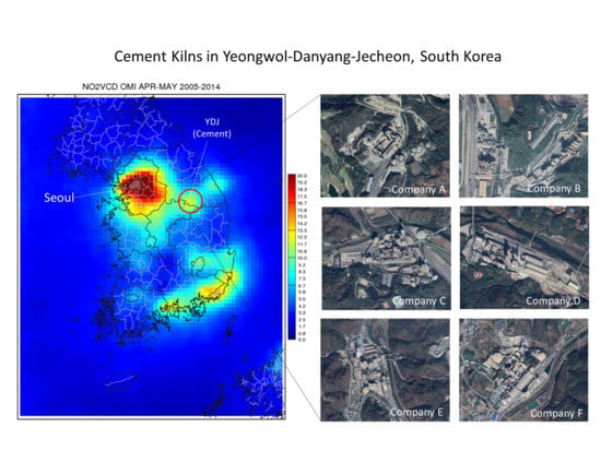
Space-Borne Monitoring of NOx Emissions from Cement Kilns in South Korea

1
Air Resources Laboratory, National Oceanic and Atmospheric Administration, College Park, MD 20740, USA
2
Cooperative Institute for Satellite Earth System Studies, University of Maryland, College Park, MD 20740, USA
3
National Air Emission Inventory and Research Center, Cheongju 28166, Korea
4
Department of Environmental and Safety Engineering, Ajou University, Suwon 16499, Korea
5
Climate and Air Quality Research Department, National Institute of Environmental Research, Incheon 22689, Korea
6
Georgia Environmental Protection Division, Atlanta, GA 30354, USA
7
Tropospheric Composition Program, National Aeronautics and Space Administration, Washington, DC 20546, USA
*
Authors to whom correspondence should be addressed.
Atmosphere 2020, 11(8), 881; https://doi.org/10.3390/atmos11080881
Submission received: 24 July 2020 / Revised: 12 August 2020 / Accepted: 13 August 2020 / Published: 18 August 2020
(This article belongs to the Special Issue Regional Air Quality Modeling)

Abstract

:
Nitrogen oxide (NOx) emissions from the South Korean cement industry are investigated with remote-sensing measurements, surface observations, and in situ aircraft measurements. In the Yeongwol, Danyang, and Jecheon regions of central South Korea, six closely located cement factories produce 31 million tons of cement annually. Their impact on the regional environment has been a public-policy issue, but their pollutants have not been continuously monitored nor have emissions inventories been fully verified. Using a newly developed downscaling technique, remote-sensing analyses show that Ozone Monitoring Instrument (OMI) NO2 column densities over the cement kilns have more than twice the modeled concentrations, indicating that the kilns are one of the most dominant NOx emission point sources in South Korea. Observed NOx emissions are stronger in the spring, suggesting that these sources play an important role in the formation of surface ozone and secondary particulate matter. These emissions also slightly increased in recent years, even while most major South Korean cities posted a declining trend in NOx emissions. Photochemical models (during May to July 2015) demonstrate that emissions from the South Korean cement industry have significant environmental impacts, both on surface ozone (up to approximately 4 ppb) and PM2.5 (up to approximately 2 µg/m3).

Graphical Abstract

1. Introduction

Cement manufacturing has serious environmental impacts at all stages of production, emitting airborne dust during the collection of raw materials in quarries and releasing kiln gases during the factory operation, among other effects. As cement is one of the most popular building materials worldwide, the cement industry is a major source of emissions, with its impacts on regional air quality and public health reported globally [1,2,3,4,5,6]. In South Korea, the impact of cement factories on nearby residents has become a public issue [7,8,9,10]. Leem et al. [11] investigated case clusters of pneumoconiosis among residents of Yeongwol, South Korea, suggesting that long-term exposure to cement dust from factories and mines may lead to the development of pneumoconiosis. Kim et al. [12] also showed that the rate of ventilation impairment in residents near cement plants is higher, likely due to their long-term exposure to particulate dust generated by these plants.
The major gaseous emission released during cement production is carbon dioxide (CO2) from the calcination process of limestone and the combustion of fuel in the kiln, accounting for around 5% of global CO2 emissions [13,14,15,16,17]. Cement kilns require a high temperature, around 2000 °C in their main burner, leading to high emissions of nitrogen oxide (NOx). Sulfur dioxide (SO2), carbon monoxide (CO), and other toxic gases are also emitted [18]. Dust emissions come during the collection of raw materials (e.g., stock piles, quarrying, and transportation) and factory operations (e.g., kiln operation, clinker cooling, and milling) [19].
Understanding the impact of emissions from cement factories requires continuous monitoring of these facilities. However, surface monitoring of emissions may be limited by the number and locations of available monitoring sites. Space-borne, remote-sensing instruments can, however, continuously monitor small-scale, local sources of emissions. In this study, we utilize the nitrogen dioxide (NO2) vertical column density (VCD) detected from space as a proxy of NOx and other emissions from the cement industry. Though NO2 itself is an important pollutant, categorized as one of the six National Ambient Air Quality Standards’ principal pollutants, it also generally indicates other emissions from the cement industry, with actual emission factors complicated by differences in fuel type [18,20,21,22].
The subsequent sections address the following: (1) Whether or not satellites can detect small-scale local emission sources, such as cement kilns; (2) whether the current South Korean emissions inventory is correct for the cement industry; and (3) whether NOx emissions signals detected by satellites are consistent with measurements by surface monitoring and aircraft. Finally, we (4) quantitatively estimate the environmental impacts of the cement industry, using both previously reported and satellite-constrained emissions. Section 2 describes the model, satellite, and data-processing methodology, and Section 3 compares the satellite-detected signals and the model. Finally, Section 4 concludes the paper.

2. Data and Methodology

2.1. Satellite

We utilized tropospheric NO2 VCD data from the Ozone Monitoring Instrument (OMI, onboard NASA’s Earth Observing System Aura satellite), specifically the Royal Netherlands Meteorological Institute’s (KNMI) DOMINO (Dutch OMI NO2) version 2.0 product obtained from the European Space Agency’s Tropospheric Emission Monitoring Internet Service (TEMIS) [23]. The OMI instrument is a nadir-viewing imaging spectrograph that measures backscattered solar radiation across a 2600 km-wide swath of the surface using a telescope with a 114° viewing angle, a measurement wavelength ranging from 270 to 500 nm, and a 0.5 nm spectral resolution. The OMI’s footprint pixel size is 13 km (along) × 24 km (across) at nadir in normal global operation mode and 13 km × 12 km in zoom mode [24]. To assure data quality, we disregarded pixels with cloud fractions over 40% or other contaminated pixels (i.e., row anomalies) using quality flags. NO2 column-retrieval algorithms and error analysis are available from Boersma et al. [25,26].

2.2. Surface Monitoring and Field Campaign

Hourly observations of NO2, PM10, SO2, and CO from surface-monitoring sites were obtained from the National Institute of Environmental Research, Korea [27]. Aircraft measurements were obtained from the KORea-United States Air Quality Study (KORUS-AQ) field campaign conducted during May to June 2016 (for detailed information on the campaign, see KORUS-AQ) [28].

2.3. Model and Emissions

A meteorology-chemistry-emission modeling framework was used to simulate tropospheric chemical components, and its simulation outputs were compared to the satellite-retrieved data. The system simulates an air-quality forecast system over East Asia (27 km) and South Korea (9 km) that has been operational since May 2012 and uses multiple configurations of meteorological and chemical models. The system comprises both forecast and hindcast systems using multiple models and has been used for various short- and long-term air-quality studies [29,30,31,32]. For the study, 11 year simulations during 2005–2015 were conducted using three emissions inventory data sets.
To simulate meteorology, this study used the Weather Research and Forecasting Model (WRF) version 3.4.1, initialized with the National Center for Environmental Protection’s final operational (FNL) global analysis data. The FNL product uses the global forecast system model with additional data assimilated using the global data assimilation system. The Community Multiscale Air Quality Model (CMAQ) [33], version 4.7.1, is used to simulate chemistry, with the Meteorology-Chemistry Interface Processor (MCIP) version 3.6 used as a preprocessor and the AERO5 aerosol module and Statewide Air Pollution Research Center version 99 (SAPRC99) [34] used as chemical mechanisms.
Regarding anthropogenic emissions for the CMAQ simulation, we used three sets of emissions inventory combinations. First, we used the Intercontinental Chemical Transport Experiment–Phase B (INTEX-B) 2006 emission inventory (http://mic.greenresource.cn/intex-b2006) [35] for all Asian countries besides South Korea; for emissions inside South Korea, we used the Clean Air Policy Support System (CAPSS) 2007. The second emission set utilizes the CAPSS 2010 emission inventory, paired with the Model Inter-Comparison Study for Asia (MICS-Asia) 2010 emission inventory [36]. Third, the CAPSS 2013 emissions inventory and the Comprehensive Regional Emissions Inventory for Atmospheric Transport Experiment (CREATE) 2013 [37] were used to represent the latest changes.
The CAPSS emission inventory has four emissions sectors: Point, area, on-road, and non-road. Categories at multiple levels for each emission sector are also available: Combustion in energy industries and in waste treatment and disposal (point); agriculture and other sources/sinks (area); non-industrial combustion plants, combustion in manufacturing industries, production processes, and storage and distribution of fuels (point and area); solvent use, other mobile sources, and machinery (mobile); and fugitive dust (mobile and area). CO, NOx, SOx, PM10, and VOCs emission for each of these upper-level categories are provided, except for fugitive-dust emissions [38]. For biogenic emissions, we used the Model of Emissions of Gases and Aerosols from Nature (MEGAN) [39]. Biomass burning and dust emissions were not included. Other studies have evaluated the general model performance [29,30,40].

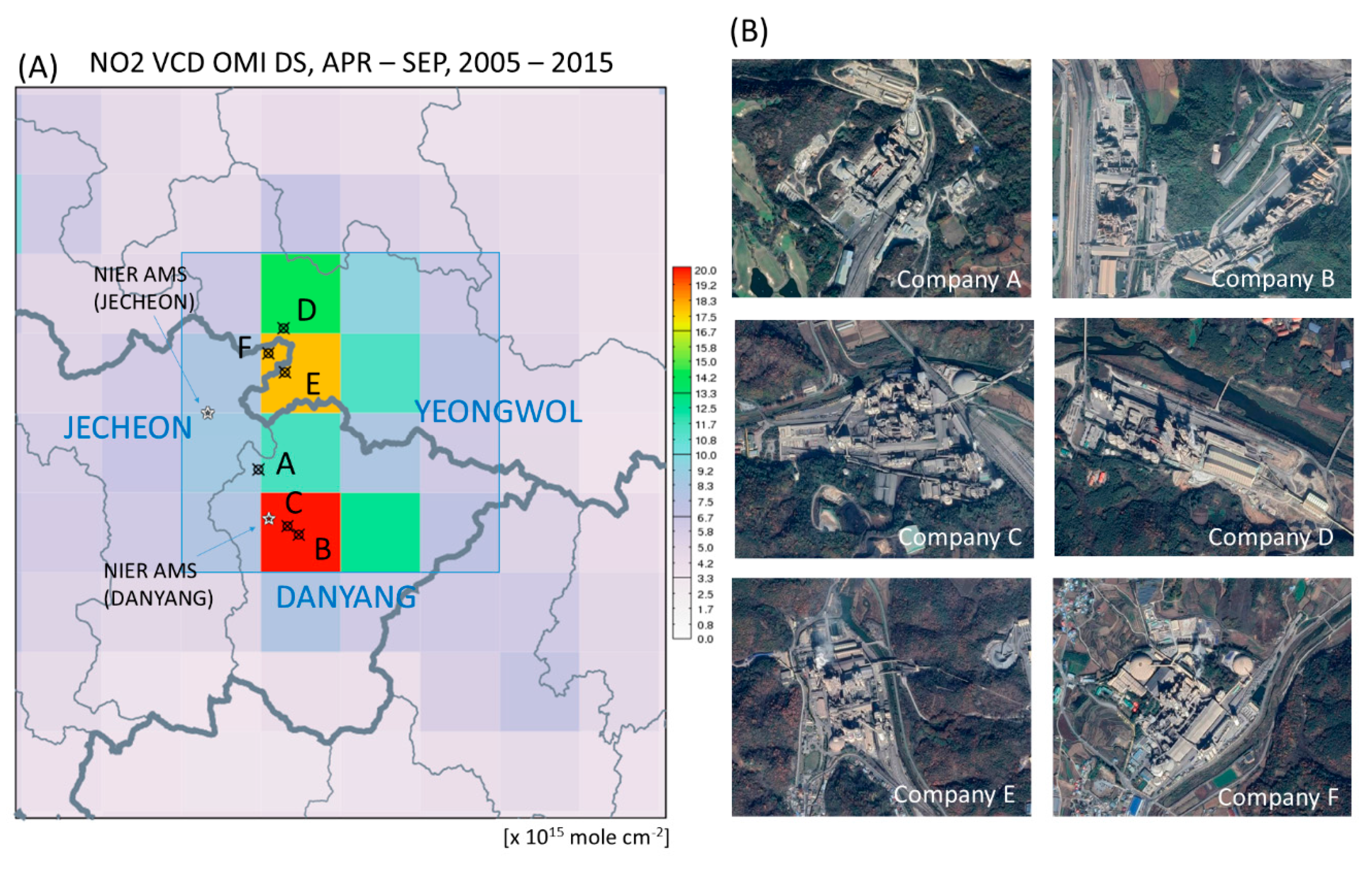
2.4. Conservative Downscaling

One common problem in comparing satellite-based NO2 observations to fine-scale NO2 simulation is that satellite-based NO2 is typically too low at rural locations and too high at urban locations [41,42,43,44]. Kim et al. [44] demonstrated that typical urban NO2 plumes are too fine for resolution in current OMI footprint pixels, causing serious bias, especially for small-scale local sources. In this study, we applied the conservative downscaling technique suggested by Kim et al. [44] to adjust systematic biases caused by geometric error in spatial sampling. This method conservatively regrids OMI observations spatially into the target domain. Each OMI pixel is reconstructed by applying a spatial-weighting kernel from the finer model simulation and then regridded into the domain grid using a fractional weighting of each portion overlapped between the OMI pixels and domain grid cells. Column densities are calculated as
C j = ( P i · K i , j ) · f i , j f i , j
where i and j are indices of data pixels, P, and grid cells, C. K i , j is a pixel-specific spatial-weighting kernel (see Figure 5 in Kim et al. [44]). The overlapping fractions, f i , j , are calculated as
f i , j = A r e a ( P i C j ) A r e a ( C j )
As spatial regridding is applied separately for each OMI pixel, strict mass conservation is guaranteed. Notably, this conservative downscaling method theoretically assures the best agreement between satellite and model by reconstructing fine-scale structures, so the differences between satellite and model in this comparison might be a lower limit on the discrepancy. Actual differences could be larger.

3. Results

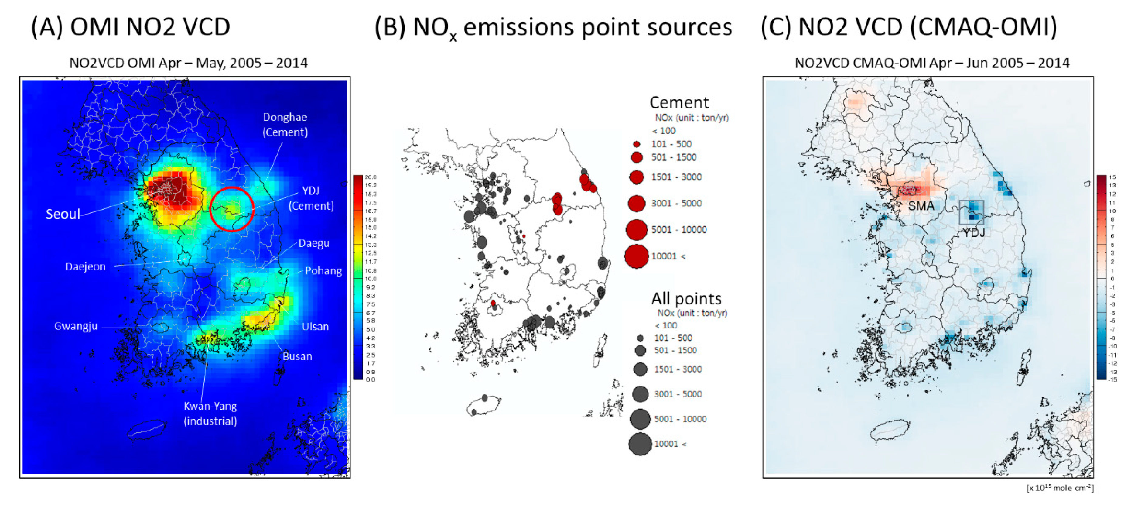
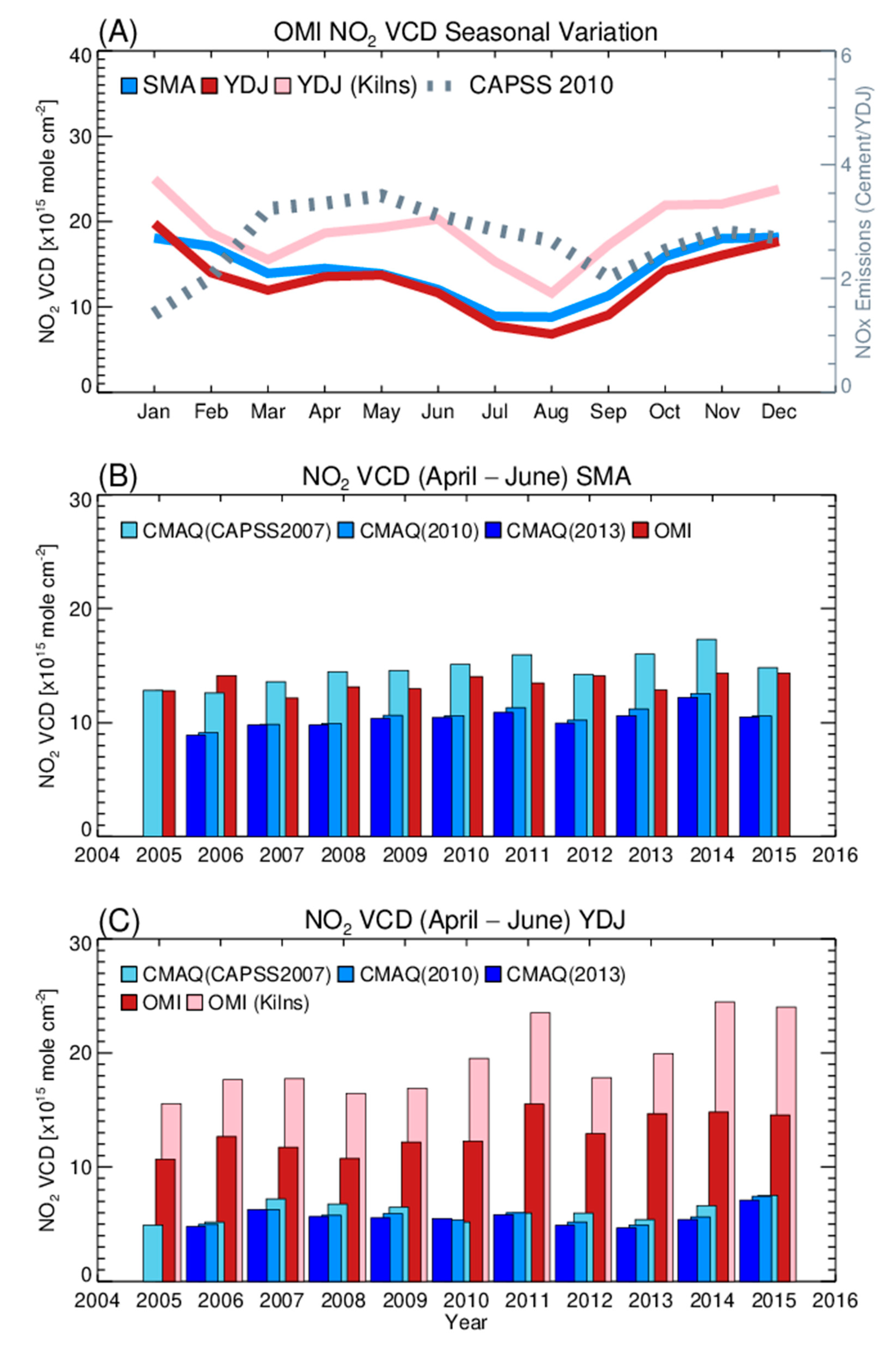
3.1. Space-Borne Monitoring

NOx emission signals from the cement industry in South Korea can be detected from OMI observations even before applying the conservative downscaling method. Figure 1A shows the spatial distribution of the OMI NO2 VCD during springtime, averaged over April to June 2005–2014, using normal spatial regridding. As mobile sources (62%), power plants (13%), and industrial sources (17%) in South Korea are all major contributors to NOx emissions [38], the general distribution of OMI NO2 VCD agrees well with the locations of major cities (e.g., Seoul, Busan, Daegu, and Gwangju), power plants (e.g., on the western coast), and industrial regions (e.g., Ulsan and Kwangyang) in the country. Geographical distributions of major point sources of NOx emissions listed in the CAPSS 2010 emissions inventory are also shown in Figure 1B for comparison with the OMI NO2 VCD distribution. Most strong point sources in the emissions inventory are recognizable from the satellite signals, although the power plants on the western coast have much weaker satellite signals than in the inventory. Interestingly, two major locations for the cement industry are well distinguishable in the OMI NO2 VCD distribution: The Yeongwol-Danyang-Jecheon (YDJ) region of central South Korea (marked with a gray box in Figure 1C), and the Donghae-Samcheok region on the eastern coast.
The OMI NO2 VCD is further compared to the modeled NO2 VCD to evaluate NOx emissions from the inventory. To remove discrepancies due to the footprint pixel-resolution issue [44,45], we applied the conservative downscaling technique as described in the methodology section above, and we also applied averaging kernel information to adjust the difference in vertical sensitivity between the satellite product and the model. Figure 1C plots the difference between the modeled NO2 VCD and OMI NO2 VCD. The modeled NO2 VCD is clearly overestimated over the Seoul Metropolitan Area (SMA) region and underestimated over several point sources, especially over the two regions where cement factories are located. This study further focuses on the YDJ region, because the signals from the Donghae-Samcheok region are likely mixed with NOx emissions from adjacent power plants.
Figure 2A shows the geographical coverage of the YDJ region. Six active companies in the region produce 31 million tons of cement every year. The amount each company produces and their estimated NOx emissions from the CAPSS 2010 inventory are listed in Table 1. Figure 2A shows zoomed-in plots of this region, showing the locations of six cement factories and two surface-monitoring sites operated by the National Institute of Environmental Research (NIER) Ambient Monitoring System (AMS) network. Locations of point sources in the current emissions inventories were confirmed using pictures from Google Earth (Figure 2B). As expected, the distributions of OMI NO2 VCD averaged over April to September, 2005–2015 likewise confirmed good agreement between the emissions inventory for the factories and satellite-observed NO2 VCD distributions.
Seasonal variation in the OMI NO2 VCD over the YDJ region also demonstrates characteristics of the cement industry. Figure 3A shows the annual variation in OMI NO2 VCD over the SMA, the YDJ, and pixels where cement kilns are located. The blue line indicates annual variation in the OMI NO2 VCD over the SMA region, which shows typical seasonal variation: High during the cold season and reaching a minimum during summer. The profile for the YDJ region shows a similar general variation but with slightly enhanced NO2 concentration during spring, when NO2 VCD becomes clearer for cells where cement kilns are located. This seasonal profile matches the annual profile of cement production; the CAPSS 2010 emissions inventory shows that cement production is highest in springtime, peaking in May (the gray dotted line in Figure 3A), likely varying with demand from the construction industry.
Figure 3B,C show the inter-annual variation in OMI NO2 VCDs over the SMA and the YDJ region. Red bars indicate OMI-observed NO2 VCD, and light and dark blue bars indicate modeled NO2 VCD using CAPSS 2007, 2010, and 2013 emission inventories, respectively. Over the SMA, NO2 VCDs simulated using information from CAPSS 2010 and CAPSS 2013 are lower than that simulated using CAPSS 2007, reflecting the impact of continuous NOx emission reduction in the SMA region, especially from the mobile sector. In spite of year-by-year variations, the OMI NO2 VCD generally agrees with these simulations, located between modeled values, implying generally good performance over the SMA. On the other hand, comparison of the modeled and satellite NO2 VCD over the YDJ region shows significant discrepancies. NO2 VCDs modeled using both CAPSS 2007 and 2010 emission inventories are just around or less than half of the satellite-measured NO2 VCDs. We noticed substantial observed springtime NO2 VCDs over the YDJ region.
Interestingly, OMI-observed NO2 VCDs over the YDJ region were as high as the SMA average, while the model seriously underestimates NO2 VCD over the six cement factories. The 11 year springtime average over the YDJ region is 12.75 × 10¹⁵ mole/cm2, slightly less than the SMA average, 13.35 × 10¹⁵ mole/cm2, but this average is much higher when counting only kiln pixels (e.g., 18.83 × 10¹⁵ mole/cm2). The yearly variation in NO2 VCD also raises an important question. During the study period, the observed OMI NO2 VCD over the YDJ region slightly increased, implying the possible addition of unknown sources of NOx emissions or degradation in the current facilities’ emissions control efficiency. We have no evidence to specify the reason for this regional increase in NO2 VCD and suggest that future studies should further investigate this change.

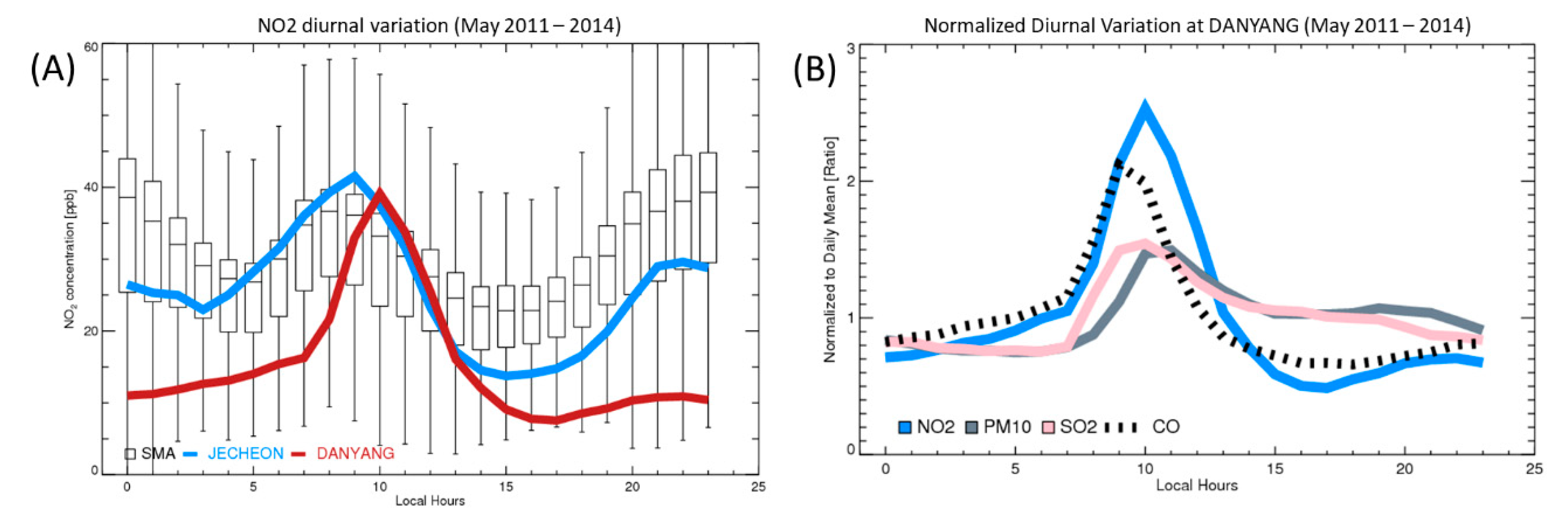
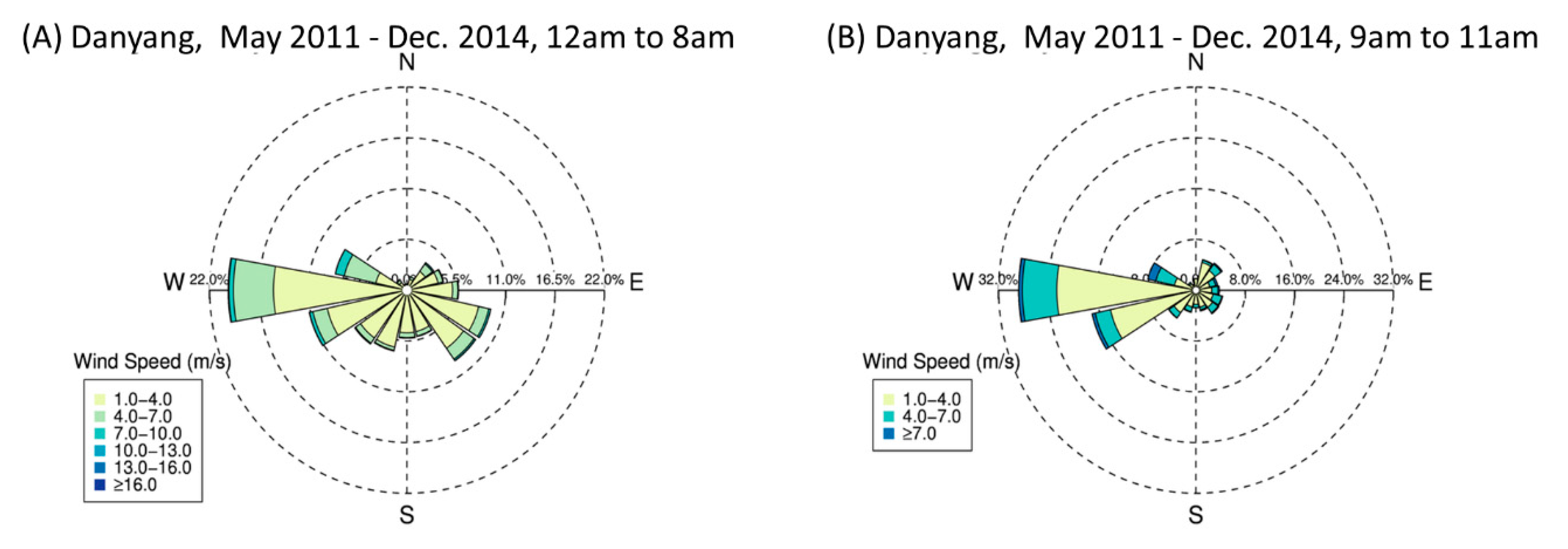
3.2. Surface Monitoring

We further examined observations from surface-monitoring sites. As mentioned above, two NIER AMS monitoring sites are available, in Jecheon and Danyang. The Jecheon site has a longer archive dating back to early 2000, whereas observations from the Danyang site are available from 2011. Figure 4 shows the diurnal variation in NO2 concentrations over the two surface monitoring sites in the YDJ region, with the distribution of SMA NO2 concentration in the whisker plot. The Jecheon site is located near road traffic, so its diurnal variation matches the typical diurnal variation in surface-monitoring sites in the SMA affected by traffic-related NOx emissions: It has two peaks, one during early rush hour near 09:00 and a second in the evening around 21:00. We therefore cannot conclude that these observations from the Jecheon site represent chemical activity from the cement factories.
The profile from the Danyang site is very different. In general, its NO2 concentration is very low compared to the concentrations from the Jecheon site or from the SMA sites. However, it shows a very high peak of emissions concentration at a specific time of the day, around 10:00. We suggest two possible reasons for this abnormal peak in the morning. First, it could be related to the intermittent operation of factory facilities. Second, we expect a typical diurnal wind direction change because this region is surrounded by mountains. Mountain-valley breeze, which happens due to the difference in thermal capacity between mountain top and valley, can cause a routine change in wind direction at a certain time of the day. If the signal were truly caused by a routine mountain breeze, surface monitors could detect emissions signals only when they are located on the downwind side of the emissions sources. Therefore, with a real emissions signal shown only in the morning, the actual emissions from cement factories at other hours of the day would be as high as the concentrations only detected in the morning, implying the real emissions would be higher than the ones inferred from the observations. While we do not have near observations of wind direction, westerly winds are dominant in the model (Figure 5).

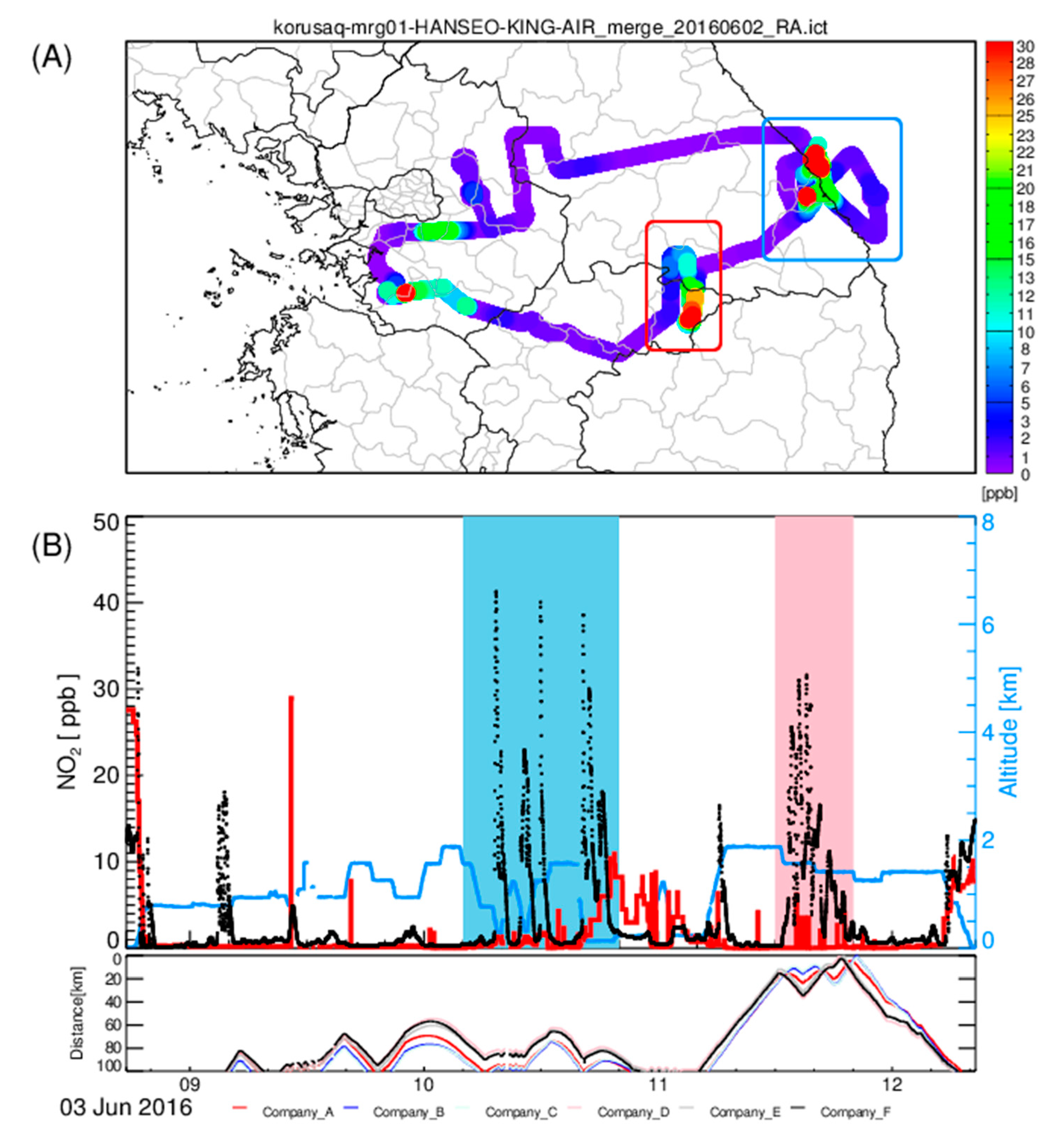
3.3. In-Situ Measurements

Additional evidence of excessive NOX emissions from the cement industry in the YDJ region is available from the KORUS-AQ field campaign measurements. Figure 6 shows the spatial distribution and time series of NO2 concentration measured by a King Air aircraft on 3 June 2016 KST. The aircraft flew over cement facilities in Donghae-Samcheock (around 10:30) and in the YDJ region (around 11:45). Over both regions, enhanced NO2 concentrations, up to 40 ppb, were observed. Over the YDJ region, especially, the NO2 concentration surpassed 30 ppb downwind of cement factories at the 1.5 km level. On the other hand, the modeled NO2 concentration (thick red line), retrieved along the flight path, shows much lower concentrations, only 30% to 50% of that observed over the YDJ region. Model concentrations only reach up to 10 ppb in the Donghae-Samcheock region, and up to 5 ppb in the YDJ region. This implies that the actual emissions rate could be more than twice as high as the current emissions inventory. This result is consistent with the satellite comparison.

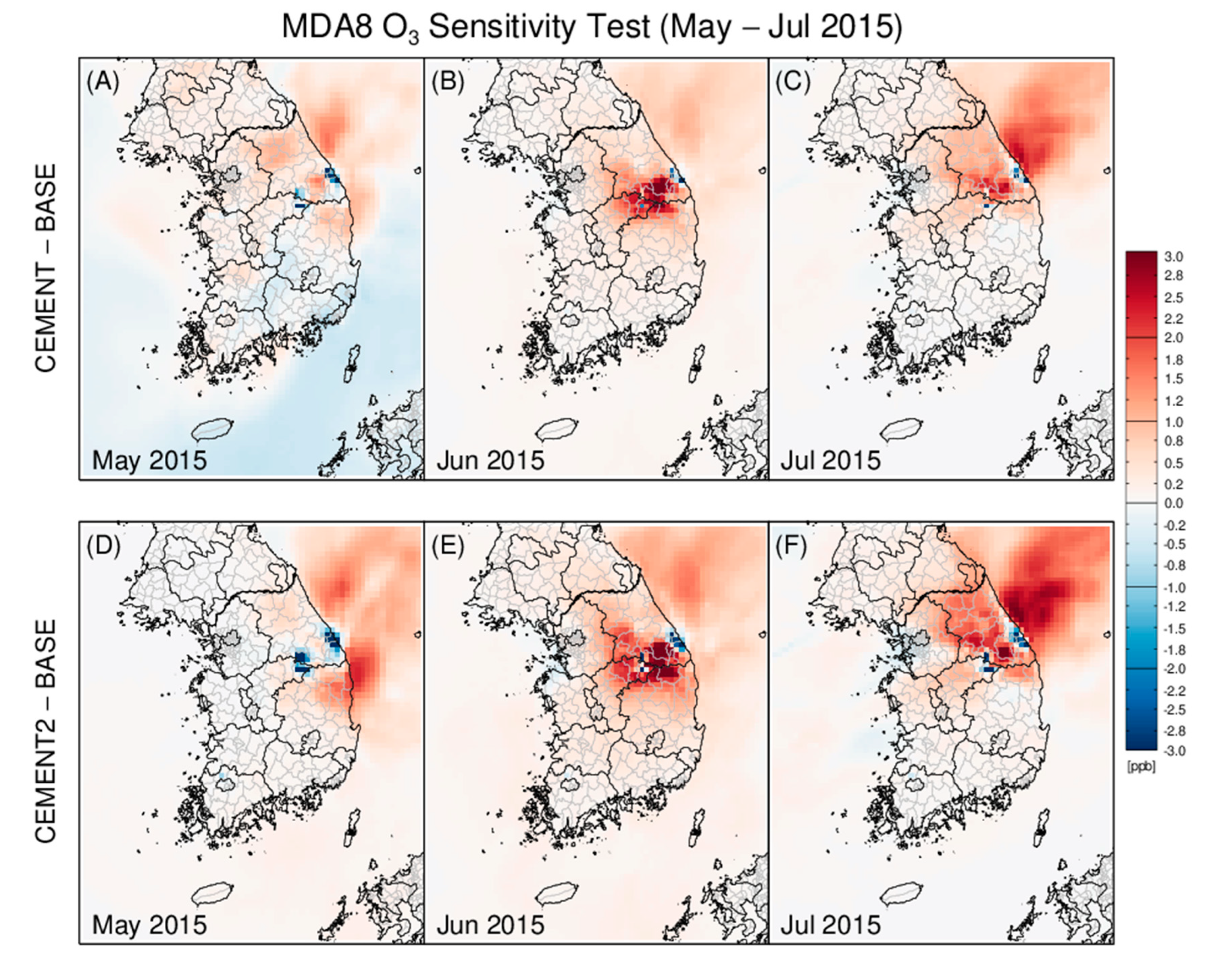
3.4. Impact Assessment by Model

We further performed photochemical transport model simulations to quantitatively demonstrate the impact of emissions from the cement industry on local and regional air quality. Three simulations—a base and two sensitivity runs—were conducted to represent the so-called known and actual impact assessments. Considering general characteristics of constructing bottom-up emissions inventories, the locations and types of released emissions from the cement industry are well-established in the CAPSS inventory. The actual amount of release, however, is always challenged by bottom-up approaches. The “BASE” simulation used CAPSS 2013 emissions, less emissions from the cement industry. The “CEMENT” simulation used the CAPSS 2013 emissions inventory, and the “CEMENT2” simulation used doubled cement emissions (i.e., CEMENT2 = BASE + (CEMENT−BASE) × 2). We decided to model doubled cement emissions based on the satellite NO2 VCD comparison described in the previous section, a decision we believe is rather conservative. We lack clear evidence that other (non-NOx) emissions are also doubled, but the synchronized behavior of other components in Figure 4B may justify the use of NO2 VCDs as indicators of the industrial activity of cement facilities.
To separate the emissions of the cement industry, we examined whole CAPSS Source Classification Codes (SCCs), identifying those codes related to the cement industry. Table 2 lists eight-digit CAPSS SCC codes related to the cement industry, with four levels of categories. In total, we have removed 32 emissions sources from CAPSS to separate emissions from the cement industry. Table 3 summarizes total emissions from the cement industry for each province in South Korea. For NOx emissions, CAPSS 2013 has eight major classification categories [46]—‘combustion in energy industries (177,219 tons/year),’ ‘Nonindustrial combustion plants (88,769 tons/year),’ ‘Combustion in manufacturing industries (178,034 tons/year),’ ‘Production processes (55,151 tons/year),’ ‘Road transport (335,721 tons/year),’ ‘Other mobile sources and machinery (246,027 tons/year),’ ‘Waste treatment and disposal (9529 tons/year),’ ‘Other sources and sinks (165 tons/year).’ Most cement industry NOx emissions belong to the industrial combustions.
Three months were simulated, May to July 2015. Figure 7 shows the impact of cement emissions on surface ozone concentration. By adding emissions from the cement industry to the base case, MDA8 ozone—the daily maximum of the eight-hour ozone moving average—showed significant changes. At the location of cement facilities, MDA8 ozone strongly decreased due to strong titration, increasing significantly in neighboring areas. Increased simulated MDA8 ozone concentrations reach as high as 3.5 and 4.1 ppb during June (for “cement” and “cement2” simulations, respectively). The impact on PM2.5 concentration is also highest during June, reaching up to 1.131.95 µg/m3 and 1.95 µg/m3 in the “cement” and “cement2” simulations, respectively (Figure 8). Depending on the wind direction, these impacts can reach the highly populated southern Gyeonggi province, and they may affect visibility in national parks (e.g., Woraksan and Sobaeksan) and fruit production in Gyeongbuk province.

4. Discussion

Because regional air quality is a serious public issue in South Korea, increasing interest has been drawn to the role of emissions from major point sources. While the impact of electricity-generating power plants drew early attention [32], the role of emissions from major industrial facilities also needs more investigation. This study investigated NOx emissions from the South Korean cement industry using remote-sensing measurements from space, surface observations, in situ aircraft measurements, and a regional chemical-transport model. We focused on the YDJ region, where six cement factories are located.
We identified NOx emissions signals from cement kilns in the YDJ region using the OMI NO2 VCD. Compared to other point sources in South Korea, the YDJ region showed one of the most dominant NO2 signals, especially during the spring. Compared to the OMI NO2 VCD, the modeled NO2 VCD is much lower in the YDJ region, implying possible underestimation of NOx emissions in this region by current emission inventories.
The findings of this study are as follows.
  • The OMI NO2 VCD detected signals from the South Korean cement industry. Additionally, application of the downscaling technique helped pinpoint small-scale, local emission sources.
  • Emission rates from the South Korean cement industry need further investigation. The model simulation can explain only half of currently observed OMI NO2 VCDs. Although this study only described NOx emissions, such emissions may indicate other emissions that could be an important subject of future research.
  • Observations from surface-monitoring sites and aircraft measurements also support the detections by satellite. We also suggest that additional, continuous surface-monitoring sites be established downwind of cement factories to monitor their emissions. On-site measurements, if available, should be made available to the public for further investigation.
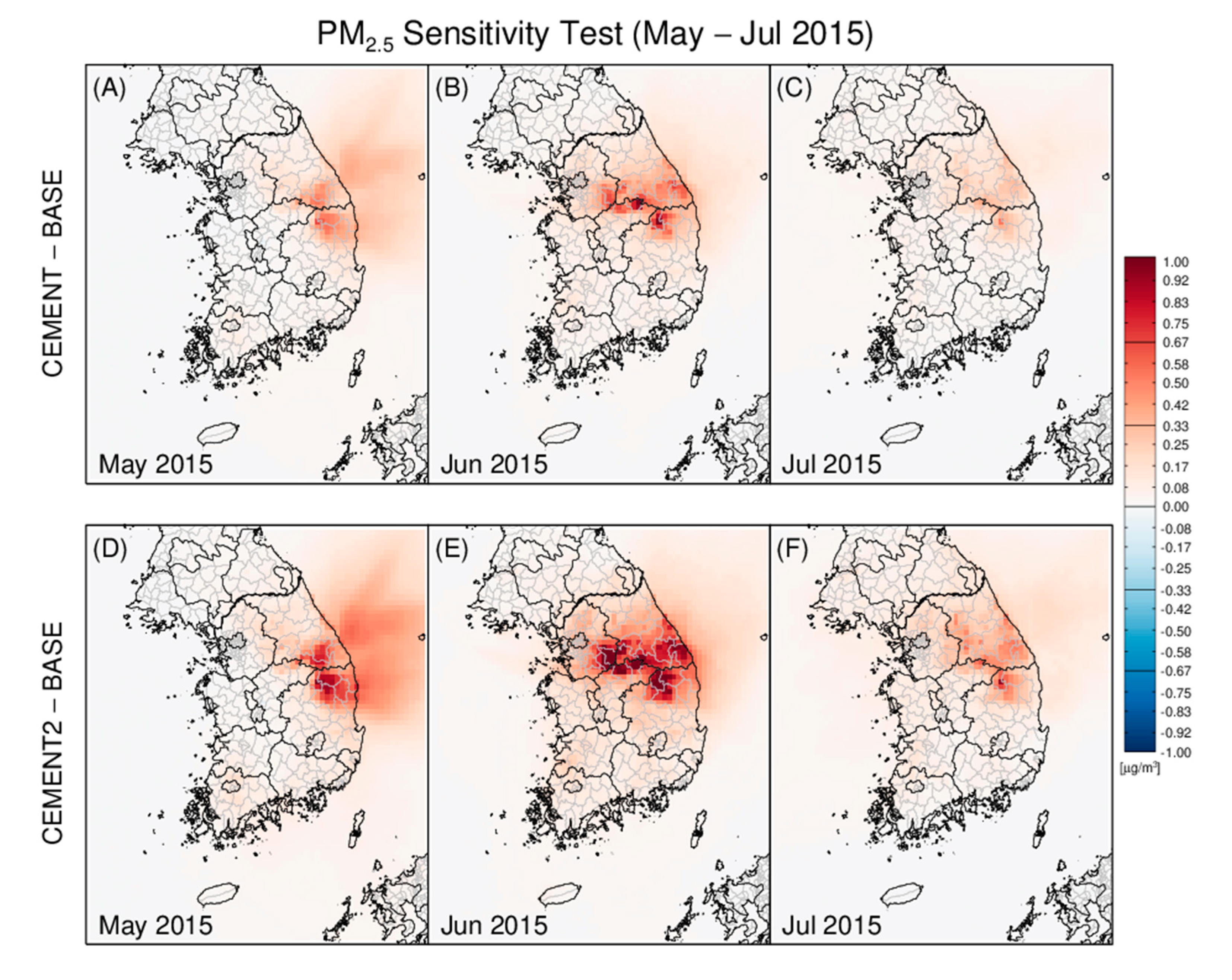
  • Modeling analyses demonstrate that cement industry emissions have significant impact even with the current emissions inventory. We estimate that actual emissions exceed current inventories by more than a factor of two, suggesting significant environmental impacts, both on surface ozone (up to approximately 4 ppb) and PM2.5 (up to approximately 2 μg/m3).
Finally, we suggest further investigation of the impact of emissions from the cement industry using a fine-resolution modeling study. As the YDJ region is surrounded by mountains, fine-scale modeling down to 3 or 1 km resolution is required to identify the real impact of those emissions. As the YDJ region is located near the center of South Korea, emissions from the cement industry could affect the SMA, southern South Korea (near Busan), Sejong City, or all these populated areas. In addition, use of more recent emissions inventories and recently launched space-borne instruments with finer observing resolutions (e.g., TROPOMI) [46] is strongly recommended.

Author Contributions

Conceptualization, H.C.K.; Data curation, C.B., M.B. and O.K.; Formal analysis, H.C.K. and O.K.; Funding acquisition, S.K.; Investigation, C.B. and M.B.; Methodology, H.C.K.; Project administration, B.L.; Resources, C.Y., J.P., J.C., J.-B.L., B.L., A.S. and S.K.; Visualization, H.C.K.; Writing—original draft, H.C.K.; Writing—review & editing, C.B., M.B., O.K., B.-U.K. and S.K. All authors have read and agreed to the published version of the manuscript.

Funding

This study was supported by the National Strategic Project-Fine Particle of the National Research Foundation of Korea (NRF) (funded by the Ministry of Science and ICT (MSIT), the Ministry of Environment (ME) and the Ministry of Health and Welfare (MOHW) (2017M3D8A1092015), South Korea, the National Air Emission Inventory and Research Center (NAIR), South Korea, and National Institute of Environmental Research (NIER-2016-03-01-006), South Korea.

Acknowledgments

We acknowledge the free use of tropospheric NO2 column data from the OMI sensor from www.temis.nl.

Conflicts of Interest

The authors declare no conflict of interest.

References

  1. Abu-Allaban, M.; Abu-Qudais, H. Impact Assessment of Ambient Air Quality by Cement Industry: A Case Study in Jordan. Aerosol Air Qual. Res. 2011, 11, 802–810. [Google Scholar] [CrossRef]
  2. Dong, Z.; Bank, M.S.; Spengler, J.D. Assessing Metal Exposures in a Community near a Cement Plant in the Northeast U.S. Int. J. Environ. Res. Public Health 2015, 12, 952–969. [Google Scholar] [CrossRef] [PubMed] [Green Version]
  3. Mehraj, S.S.; Bhat, G.A.; Balkhi, H.M.; Gul, T. Health risks for population living in the neighborhood of a cement factory. Afr. J. Environ. Sci. Technol. 2013, 7, 1044–1052. [Google Scholar] [CrossRef]
  4. Oguntoke, O.; Awanu, A.E.; Annegarn, H.J. Impact of cement factory operations on air quality and human health in Ewekoro Local Government Area, South-Western Nigeria. Int. J. Environ. Stud. 2012, 69, 934–945. [Google Scholar] [CrossRef]
  5. Rovira, J.; Flores, J.; Schuhmacher, M.; Nadal, M.; Domingo, J.L. Long-Term Environmental Surveillance and Health Risks of Metals and PCDD/Fs Around a Cement Plant in Catalonia, Spain. Hum. Ecol. Risk Assess. An Int. J. 2015, 21, 514–532. [Google Scholar] [CrossRef] [Green Version]
  6. Schuhmacher, M.; Domingo, J.L.; Garreta, J. Pollutants emitted by a cement plant: Health risks for the population living in the neighborhood. Environ. Res. 2004, 95, 198–206. [Google Scholar] [CrossRef]
  7. Cho, S.H.; Kim, H.W.; Han, Y.J.; Kim, W.J. Characteristics of Fine Particles Measured in Two Different Functional Areas and Identification of Factors Enhancing Their Concentrations. J. Korean Soc. Atmos. Environ. 2016, 32, 100–113. [Google Scholar] [CrossRef]
  8. Han, Y.J.; Kim, H.W.; Cho, S.H.; Kim, P.R.; Kim, W.J. Metallic elements in PM2.5 in different functional areas of Korea: Concentrations and source identification. Atmos. Res. 2015, 153, 416–428. [Google Scholar] [CrossRef]
  9. Lee, H.S.; Lee, C.G.; Kim, D.H.; Song, H.S.; Jung, M.S.; Kim, J.Y.; Park, C.H.; Ahn, S.C.; Yu, S. Do Emphysema prevalence related air pollution caused by a cement plant. Ann. Occup. Environ. Med. 2016, 28, 17. [Google Scholar] [CrossRef] [Green Version]
  10. Won, J.H.; Lee, T.G. Estimation of total annual mercury emissions from cement manufacturing facilities in Korea. Atmos. Environ. 2012, 62, 265–271. [Google Scholar] [CrossRef]
  11. Leem, J.H.; Kim, S.T.; Kim, H.C. Public-health impact of outdoor air pollution for 2(nd) air pollution management policy in Seoul metropolitan area, Korea. Ann. Occup. Environ. Med. 2015, 27, 7. [Google Scholar] [CrossRef] [PubMed] [Green Version]
  12. Kim, S.H.; Lee, C.G.; Song, H.S.; Lee, H.S.; Jung, M.S.; Kim, J.Y.; Park, C.H.; Ahn, S.C.; Yu, S. Do Ventilation impairment of residents around a cement plant. Ann. Occup. Environ. Med. 2015, 27, 3. [Google Scholar] [CrossRef] [Green Version]
  13. Andres, R.J.; Marland, G.; Fung, I.; Matthews, E. A 1° × 1° distribution of carbon dioxide emissions from fossil fuel consumption and cement manufacture, 1950–1990. Glob. Biogeochem. Cycles 1996, 10, 419–429. [Google Scholar] [CrossRef]
  14. Benhelal, E.; Zahedi, G.; Shamsaei, E.; Bahadori, A. Global strategies and potentials to curb CO2 emissions in cement industry. J. Clean. Prod. 2013, 51, 142–161. [Google Scholar] [CrossRef]
  15. Ke, J.; McNeil, M.; Price, L.; Khanna, N.Z.; Zhou, N. Estimation of CO2 emissions from China’s cement production: Methodologies and uncertainties. Energy Policy 2013, 57, 172–181. [Google Scholar] [CrossRef] [Green Version]
  16. Wang, Y.; Zhu, Q.; Geng, Y. Trajectory and driving factors for GHG emissions in the Chinese cement industry. J. Clean. Prod. 2013, 53, 252–260. [Google Scholar] [CrossRef]
  17. Worrell, E.; Price, L.; Martin, N.; Hendriks, C.; Meida, L.O. CARBON D IOXIDE E MISSIONS FROM THE G LOBAL C EMENT I NDUSTRY 1. Annu. Rev. Energy Environ. 2001, 26, 303–329. [Google Scholar] [CrossRef]
  18. Conesa, J.A.; Gálvez, A.; Mateos, F.; Martín-Gullón, I.; Font, R. Organic and inorganic pollutants from cement kiln stack feeding alternative fuels. J. Hazard. Mater. 2008, 158, 585–592. [Google Scholar] [CrossRef]
  19. Huntzinger, D.N.; Eatmon, T.D. A life-cycle assessment of Portland cement manufacturing: Comparing the traditional process with alternative technologies. J. Clean. Prod. 2009, 17, 668–675. [Google Scholar] [CrossRef]
  20. Schuhmacher, M.; Nadal, M.; Domingo, J.L. Environmental monitoring of PCDD/Fs and metals in the vicinity of a cement plant after using sewage sludge as a secondary fuel. Chemosphere 2009, 74, 1502–1508. [Google Scholar] [CrossRef]
  21. Rovira, J.; Mari, M.; Nadal, M.; Schuhmacher, M.; Domingo, J.L. Partial replacement of fossil fuel in a cement plant: Risk assessment for the population living in the neighborhood. Sci. Total Environ. 2010, 408, 5372–5380. [Google Scholar] [CrossRef] [PubMed]
  22. Prisciandaro, M.; Mazziotti, G.; Veglió, F. Effect of burning supplementary waste fuels on the pollutant emissions by cement plants: A statistical analysis of process data. Resour. Conserv. Recycl. 2003, 39, 161–184. [Google Scholar] [CrossRef]
  23. TEMIS. Available online: http://www.temis.nl/airpollution/no2.html (accessed on 17 August 2020).
  24. Levelt, P.; van den Oord, G.H.J.; Dobber, M.R.; Malkki, A.; Stammes, P.; Lundell, J.O.V.; Saari, H. The ozone monitoring instrument. IEEE Trans. Geosci. Remote Sens. 2006, 44, 1093–1101. [Google Scholar] [CrossRef]
  25. Boersma, K.F.; Eskes, H.J.; Brinksma, E.J. Error analysis for tropospheric NO2 retrieval from space. J. Geophys. Res. 2004, 109, D04311. [Google Scholar] [CrossRef]
  26. Boersma, K.F.; Eskes, H.J.; Veefkind, J.P.; Brinksma, E.J.; van der A, R.J.; Sneep, M.; van den Oord, G.H.J.; Levelt, P.F.; Stammes, P.; Gleason, J.F.; et al. Near-real time retrieval of tropospheric NO2 from OMI. Atmos. Chem. Phys. 2007, 7, 2103–2118. [Google Scholar] [CrossRef] [Green Version]
  27. AirKorea. Available online: https://www.airkorea.or.kr/index (accessed on 17 August 2020).
  28. KORUS-AQ. Available online: https://espo.nasa.gov/korus-aq/content/KORUS-AQ (accessed on 17 August 2020).
  29. Kim, H.C.; Kim, E.; Bae, C.; Cho, J.H.; Kim, B.-U.; Kim, S. Regional contributions to particulate matter concentration in the Seoul metropolitan area, South Korea: Seasonal variation and sensitivity to meteorology and emissions inventory. Atmos. Chem. Phys. 2017, 17, 10315–10332. [Google Scholar] [CrossRef] [Green Version]
  30. Kim, H.C.; Kim, S.; Kim, B.-U.; Jin, C.-S.; Hong, S.; Park, R.; Son, S.-W.; Bae, C.; Bae, M.; Song, C.-K.; et al. Recent increase of surface particulate matter concentrations in the Seoul Metropolitan Area, Korea. Sci. Rep. 2017, 7, 4710. [Google Scholar] [CrossRef] [Green Version]
  31. Kim, B.-U.; Bae, C.; Kim, H.C.; Kim, E.; Kim, S. Spatially and chemically resolved source apportionment analysis: Case study of high particulate matter event. Atmos. Environ. 2017, 162, 55–70. [Google Scholar] [CrossRef]
  32. Kim, B.-U.; Kim, O.; Kim, H.C.; Kim, S. Influence of fossil-fuel power plant emissions on the surface fine particulate matter in the Seoul Capital Area, South Korea. J. Air Waste Manag. Assoc. 2016, 66, 863–873. [Google Scholar] [CrossRef] [Green Version]
  33. Byun, D.; Schere, K.L. Review of the Governing Equations, Computational Algorithms, and Other Components of the Models-3 Community Multiscale Air Quality (CMAQ) Modeling System. Appl. Mech. Rev. 2006, 59, 51. [Google Scholar] [CrossRef]
  34. Carter, W.P.L. Documentation of the SAPRC-99 Chemical Mechanism for VOC Reactivity Assessment. Assessment 1999, 1, 329. [Google Scholar]
  35. Zhang, Q.; Streets, D.G.; Carmichael, G.R.; He, K.B.; Huo, H.; Kannari, A.; Klimont, Z.; Park, I.S.; Reddy, S.; Fu, J.S.; et al. Asian emissions in 2006 for the NASA INTEX-B mission. Atmos. Chem. Phys. 2009, 9, 5131–5153. [Google Scholar] [CrossRef] [Green Version]
  36. Li, M.; Zhang, Q.; Kurokawa, J.; Woo, J.-H.; He, K.; Lu, Z.; Ohara, T.; Song, Y.; Streets, D.G.; Carmichael, G.R.; et al. MIX: A mosaic Asian anthropogenic emission inventory under the international collaboration framework of the MICS-Asia and HTAP. Atmos. Chem. Phys. 2017, 17, 935–963. [Google Scholar] [CrossRef] [Green Version]
  37. Jang, Y.; Lee, Y.; Kim, J.; Kim, Y.; Woo, J.-H. Improvement China Point Source for Improving Bottom-Up Emission Inventory. Asia-Pac. J. Atmos. Sci. 2019. [Google Scholar] [CrossRef]
  38. Lee, D.; Lee, Y.-M.; Jang, K.-W.; Yoo, C.; Kang, K.-H.; Lee, J.-H.; Jung, S.-W.; Park, J.-M.; Lee, S.-B.; Han, J.-S.; et al. Korean National Emissions Inventory System and 2007 Air Pollutant Emissions. Asian J. Atmos. Environ. 2011, 5, 278–291. [Google Scholar] [CrossRef] [Green Version]
  39. Guenther, A.; Karl, T.; Harley, P.; Wiedinmyer, C.; Palmer, P.I.; Geron, C. Estimates of global terrestrial isoprene emissions using MEGAN (Model of Emissions of Gases and Aerosols from Nature). Atmos. Chem. Phys. 2006, 6, 3181–3210. [Google Scholar] [CrossRef] [Green Version]
  40. Kim, E.; Kim, B.-U.; Kim, H.; Kim, S. The Variability of Ozone Sensitivity to Anthropogenic Emissions with Biogenic Emissions Modeled by MEGAN and BEIS3. Atmosphere 2017, 8, 187. [Google Scholar] [CrossRef] [Green Version]
  41. Napelenok, S.L.; Pinder, R.W.; Gilliland, A.B.; Martin, R.V. A method for evaluating spatially-resolved NOx emissions using Kalman filter inversion, direct sensitivities, and space-based NO2 observations. Atmos. Chem. Phys. 2008, 8, 5603–5614. [Google Scholar] [CrossRef] [Green Version]
  42. Beirle, S.; Platt, U.; Wenig, M.; Wagner, T. Highly resolved global distribution of tropospheric NO2 using GOME narrow swath mode data. Atmos. Chem. Phys. 2004, 4, 1913–1924. [Google Scholar] [CrossRef] [Green Version]
  43. Hilboll, A.; Richter, A.; Burrows, J.P. Long-term changes of tropospheric NO2 over megacities derived from multiple satellite instruments. Atmos. Chem. Phys. 2013, 13, 4145–4169. [Google Scholar] [CrossRef] [Green Version]
  44. Kim, H.C.; Lee, P.; Judd, L.; Pan, L.; Lefer, B. OMI NO2 column densities over North American urban cities: The effect of satellite footprint resolution. Geosci. Model Dev. 2016, 9, 1111–1123. [Google Scholar] [CrossRef] [Green Version]
  45. Valin, L.C.; Russell, A.R.; Hudman, R.C.; Cohen, R.C. Effects of model resolution on the interpretation of satellite NO2 observations. Atmos. Chem. Phys. 2011, 11, 11647–11655. [Google Scholar] [CrossRef] [Green Version]
  46. Kim, H.C.; Kim, S.; Lee, S.-H.; Kim, B.-U.; Lee, P. Fine-Scale Columnar and Surface NOx Concentrations over South Korea: Comparison of Surface Monitors, TROPOMI, CMAQ and CAPSS Inventory. Atmosphere 2020, 11, 101. [Google Scholar] [CrossRef] [Green Version]
Figure 1. Spatial distributions of (A) Ozone Monitoring Instrument (OMI) NO2 volume column density (VCD), (B) NOx emissions from the Clean Air Policy Support System (CAPSS) 2010 emission inventory, and (C) difference in NO2 VCD between Community Multiscale Air Quality Model (CMAQ) (with averaging kernel) and OMI (downscaling applied). See the body of the paper for details about the averaging kernel and downscaling techniques. The gray box indicates the YDJ region.
Atmosphere 11 00881 g001
Figure 2. (A) Geographical locations of six cement factories in the Yeongwol-Danyang-Jecheon (YDJ) region and of National Institute of Environmental Research (NIER) Ambient Monitoring System (AMS) surface-monitoring sites (Jecheon and Danyang) over the OMI NO2 VCD distribution (April–September average from 2005 to 2015, Downscaled). (B) Satellite pictures of factories.
Atmosphere 11 00881 g002
Figure 3. (A) Annual variation in OMI NO2 VCD over the Seoul Metropolitan Area (SMA), YDJ, YDJ (kilns), and YDJ NOx emissions (six cement kilns, CAPSS 2010). Inter-annual changes in OMI and CMAQ NO2 VCDs (April to June 2005–2015) (B) over the SMA and (C) over the YDJ.
Atmosphere 11 00881 g003
Figure 4. (A) Diurnal variation in NO2 concentrations from surface monitors over the Jecheon (blue), Danyang (red), and the SMA (whisker boxes) regions, and (B) normalized diurnal variations from the Danyang site for NO2, PM10, SO2, and CO concentrations.
Atmosphere 11 00881 g004
Figure 5. Wind rose analyses from the Weather Research and Forecasting (WRF) model at the location of Danyang surface-monitoring site. (A) Nighttime (12am to 8am) and (B) morning time (9am to 11am) analyses are presented.
Atmosphere 11 00881 g005
Figure 6. (A) Spatial distribution and (B) time series of NO2 concentration measured by King-Air aircraft on 3 June 2016 during the KORea-United States Air Quality Study (KORUS-AQ) field campaign. The thick red line shows modeled NO2 concentrations from the CMAQ model. Distances from the aircraft to six YDJ cement factories are shown in the bottom panel.
Atmosphere 11 00881 g006
Figure 7. Impact of emissions from the cement industry on MDA8 O3 during May to July 2015. Simulated impacts are shown based on the current CAPSS 2013 emissions inventory (AC) and satellite measurements (DF).
Atmosphere 11 00881 g007
Figure 8. Impact of emissions by the cement industry on monthly averaged PM2.5 concentration during May to July 2015. Simulated impacts are shown based on the current CAPSS 2013 emissions inventory (AC) and satellite measurements (DF).
Atmosphere 11 00881 g008
Table 1. Six cement factories in the YDJ region, listed with number of kilns, production capacity, and NOx emissions (CAPSS 2010) from each factory.
RegionDanyangYeongwolJecheon
CompanyABCDEF
Kilns456254
Capacity
(tons/year)
2,904,0009,686,0007,131,0003,960,0003,537,0004,146,000
NOx Emission
(tons/year)
CAPSS 2007119576506185683935605312
CAPSS 201078596525129708939465448
CAPSS 2013103689137579692638127863
Table 2. CAPSS Source Classification Codes corresponding to emissions by the cement industry.
CodeSCC1SCC2SCC3SCC4
03021300Industrial CombustionFurnaceCement
03022000Industrial CombustionFurnaceMisc.
03010100Industrial CombustionCombustion facilities1–3 class boiler
04990201Industrial processesMisc. manufacturingCement
(Carbon removing)
Point source
04080202Industrial processesAmmonia consumptionSNCRIndustrial
09010201Waste disposalWaste incineratorIndustrial waste<200 kg/h
Table 3. Emissions from the cement industry in the CAPSS 2013 emissions inventory.
ProvincesCONOxVOCNH3SOxPM10PM2.5PMC
Gangwon-do76740,97392936847833565
Chungcheongbuk-do6325,63745438851206172
Chungcheongnam-do8231
Jeollabuk-do 3 2
Jeollnam-do2210363 7851

