Gravity Wave Investigations over Comandante Ferraz Antarctic Station in 2017: General Characteristics, Wind Filtering and Case Study

Abstract

This work presents the characteristics of gravity waves observed over Comandante Ferraz Antarctic Station (EACF: 62.1° S, 58.4° W). A total of 122 gravity waves were observed in 34 nights from March to October 2017, and their parameters were obtained by using the Fourier Transform spectral analysis. The majority of the observed waves presented horizontal wavelength ranging from 15 to 35 km, period from 5 to 20 min, and horizontal phase speed from 10 to 70 ± 2 m·s⁻¹. The propagation direction showed an anisotropic condition, with the slower wave propagating mainly to the west, northwest and southeast directions, while the faster waves propagate to the east, southeast and south. Blocking diagrams for the period of April–July showed a good agreement between the wave propagation direction and the blocking positions, which are eastward oriented while the waves propagate mainly westward. A case study to investigate wave sources was conducted for the night of 20–21 July, wherein eight small-scale and one medium-scale gravity waves were identified. Reverse ray tracing model was used to investigate the gravity wave source, and the results showed that six among eight small-scale gravity waves were generated in the mesosphere. On the other hand, only two small-scale waves and the medium-scale gravity wave had likely tropospheric or stratospheric origin, however, they could not be associated with any reliable source.

1. Introduction

Atmospheric gravity waves (GWs) are considered to play an important role in the transport of energy and momentum, coupling the distinct atmospheric layers, contributing to the mix of mass and modifications in temperature and global circulation processes. The distribution of energy is conducted more rapidly by waves than by the mean flow. Wave transport and subsequent deposition of energy are an important component of the atmospheric dynamics [1]. Upward propagating gravity waves transport energy and momentum and deposit them to the mean background flow during wave breaking and filtering [2,3].

Gravity waves generated in the troposphere/lower stratosphere are due to the flow above orographic structures (ridges, high isolated mountains), or other instabilities caused by convection, wind shears, jet streams or wave–wave interactions [3,4,5]. While a wave propagates upward, it is affected by the mean wind and can be blocked by wind in a region known as “critical level” [6]. Some of the waves generated in lower layers of the atmosphere can propagate all over the atmosphere gaining altitude, while grows in amplitude, and can reach the upper mesosphere and thermosphere without being filtered by the wind [7,8,9]. The critical level is a layer, or an altitude level, where the wind velocity in the wave propagation direction becomes close (or equal) to the GW phase velocity.

It is well known that gravity waves play an important role at lower levels of the atmosphere and influence weather and meteorological phenomena [10]. Some studies demonstrated the importance of applying gravity wave models to improve the accuracy of weather forecast and global circulation models [11,12].

The Antarctic Peninsula shows an intense gravity wave activity, which is observed at the altitudes ranging from the troposphere (about 5 to 10 km) to the mesosphere and lower thermosphere (about 80 to 100 km) [13,14,15,16,17]. Recent works have used winds from meteor radar and models in order to calculate the waves intrinsic parameters; to investigate the environment conditions in which the waves propagate vertically; to estimate the momentum and energy fluxes; to analyze the influence of gravity waves in the solar tidal oscillations or mixed tide–gravity wave mode [18,19,20,21,22,23].

In this work we study the characteristics of the gravity waves observed by an airglow imager over the Brazilian Antarctic Station, Comandante Ferraz Antarctic Station (EACF, or Ferraz Station), during the year of 2017. We also investigate the possible occurrence of wind filtering using blocking diagrams. The gravity waves were observed and analyzed by using airglow images, while the data set of winds was obtained from the ERA-5 reanalysis and from a nearby meteor radar operated at the King Sejong Station (KSS) at King George Island. This work investigates wind filtering and potential wave source regions during one night with high gravity wave activity. A case study of small and medium scale gravity waves was also conducted.

Results in terms of gravity wave characteristics are quite well known for the Antarctic region. The main contribution of this work is to study the wave propagation by using blocking diagrams of nocturnal averaged winds in selected periods of days. In addition, the work is complemented by blocking diagrams and ray tracing results which are compatible in terms of the generation and propagation of the investigated waves.

2. Instrumentation and Methodology

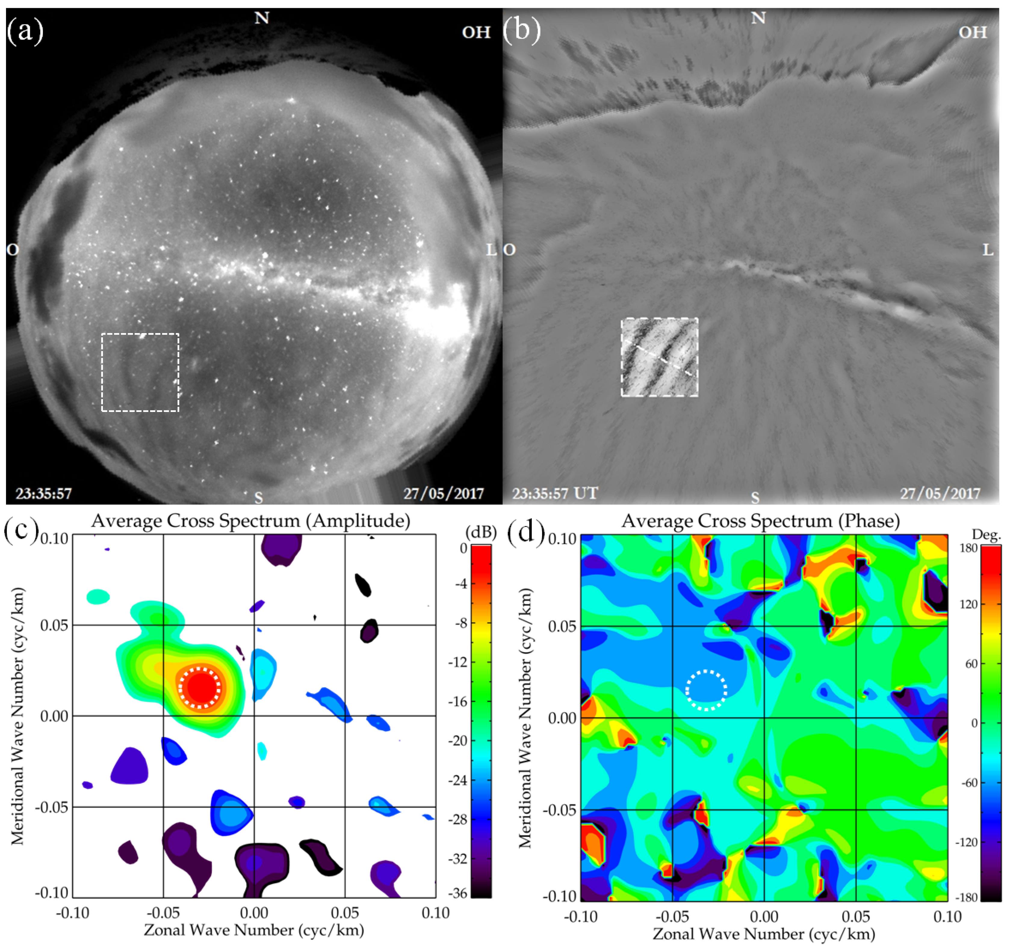
2.1. Airglow All-Sky Imager and Data Analysis

Gravity waves were observed by using an all-sky imager installed at Comandante Ferraz Antarctic Station–EACF (62.1° S, 58.4° W), located on King George Island, Antarctic Peninsula. Airglow observations were taken, with at least 2 h of clear sky conditions, from March to October 2017. The all-sky imager is composed of a telecentric lens system, a fish-eye lens, and a six-position 3 inches filter wheel, with three airglow filters, to measure Hydroxyl-Near Infrared (OH-NIR), atomic oxygen green (5577 Å) and red (6300 Å) lines. The imager has also a Charge Coupled Device (CCD) with quantum efficiency greater than 95% in the visible light spectrum and thermoelectric cooling down to −70 °C. More details on the specifications of the airglow imager are found at the Keoscientific web page: Available online: http://www.keoscientific.com/aeronomy-imagers.php (accessed on 20 March 2020).

In order to analyze the airglow images to obtain the wave parameters, a sequence of procedures is performed, as follows: (1) the original image is unwarped and then mapped into the geographical coordinates [24]; (2) a digital pre-processing is applied in the images in order to remove the star field and the lower frequencies (Bageston, 2011 [25]); (3) a region of interest (ROI) is selected in the unwarped image where the gravity wave is observed; (4) spectral analysis is applied in the ROI for a sequence of images, following the methodology described by Wrasse et al. (2007) [26]. The spectral analysis consists of a 2-dimensional Fast Fourier Transform (2-D FFT, or just FFT). The amplitude and phase spectra, obtained from the Fourier Transform, are used to calculate the wave parameters such as horizontal wavelength, observed period, horizontal phase speed and propagation direction, without any ambiguity.

Figure 1 shows an example of airglow image and summarizes the spectral analysis method. Figure 1a,b show, respectively, a selected gravity wave in the original all-sky image and the wave in the unwarped, mapped, and filtered image. For the spectral analysis a sequence of four images were taken, and the averaged spectrum is obtained. Figure 1c,d present the unambiguous cross spectra and phase, respectively, resulted from the two-dimensional FFT analysis applied to a set of images observed between 23:32 and 23:37 UT on the night of 27 May 2017.

The gravity wave analyzed in Figure 1 presented a horizontal wavelength of 30.1 ± 0.7 km, observed period of 18.8 ± 1.5 min, horizontal phase speed of 26.7 ± 2 m·s⁻¹, and was propagating in the northwest direction (azimuth of 298.1°). More details on gravity wave parameter calculation can be found in Wrasse et al. (2007) [26].

Uncertainties in the gravity wave parameters were estimated by taking the standard deviation of the horizontal wavelength calculated for each individual image at the same wavenumber. Applying the propagation error theory (Bevington and Robinson, 2002. [27]) the other uncertainties were also estimated. In general, the uncertainty of the horizontal wavelength was lower than 10% of the horizontal wavelength. Another source of uncertainty was the ROI, in which different ROI’s may have resulted in slightly different gravity wave parameters.

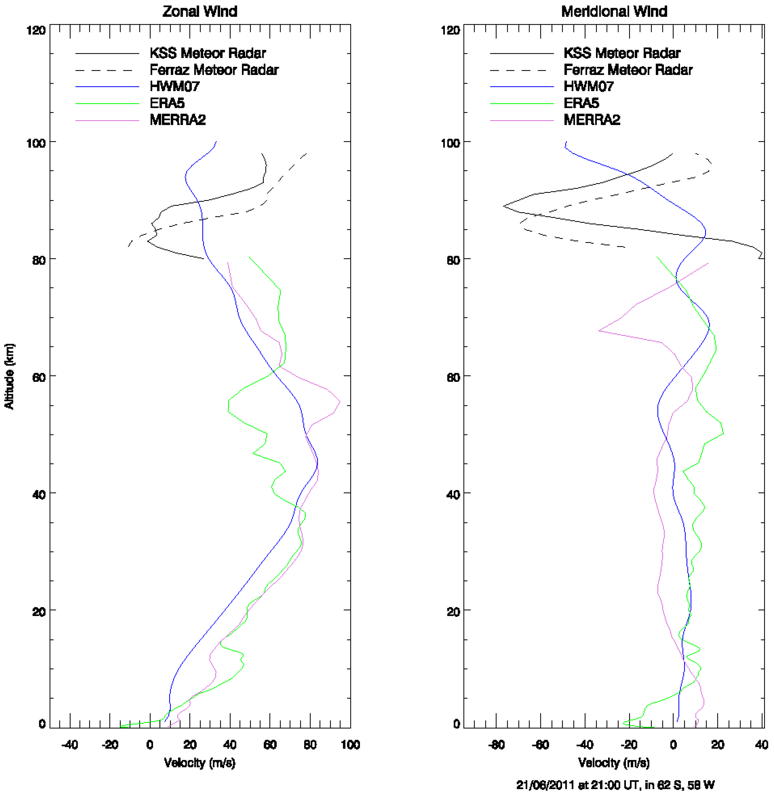
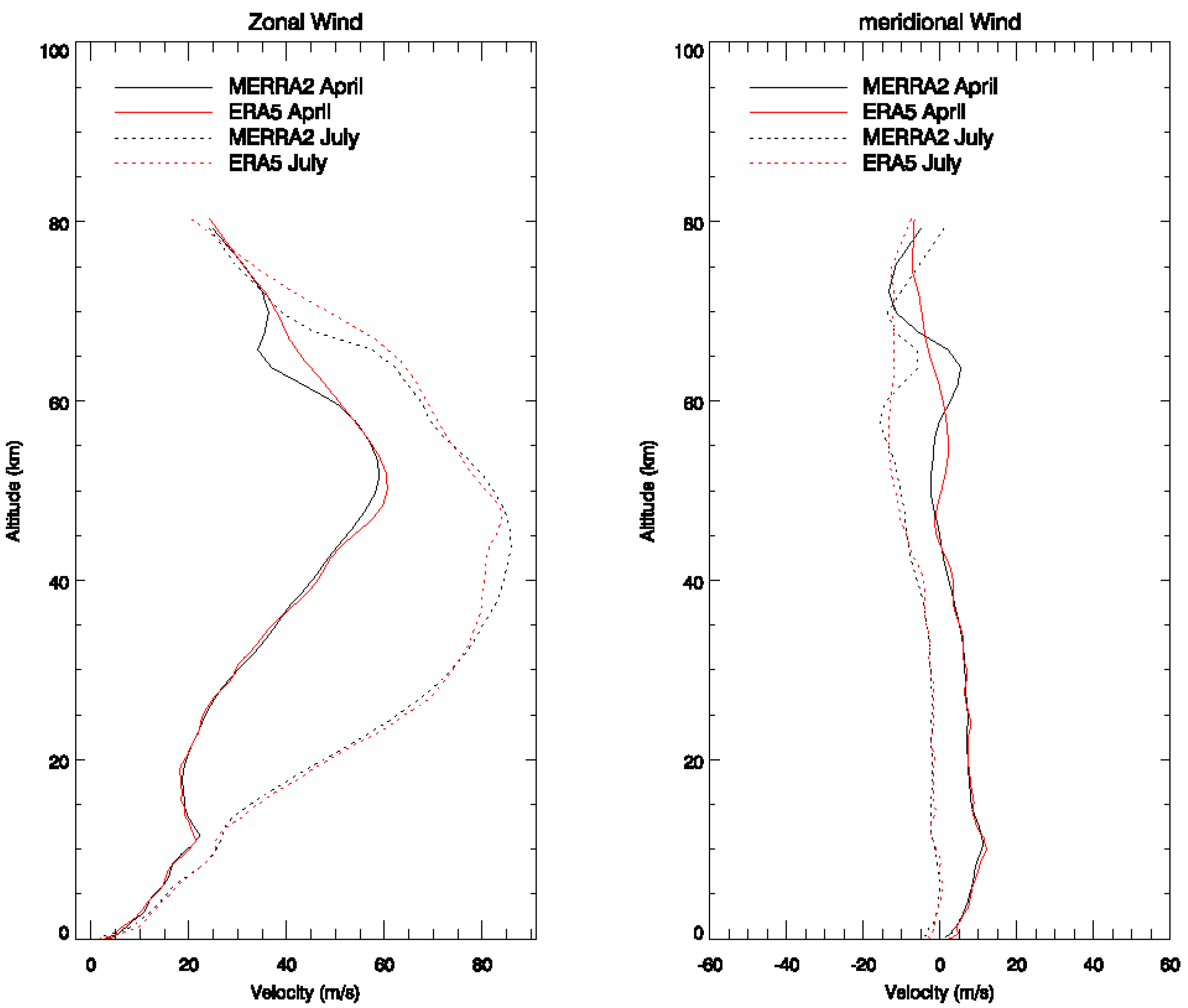
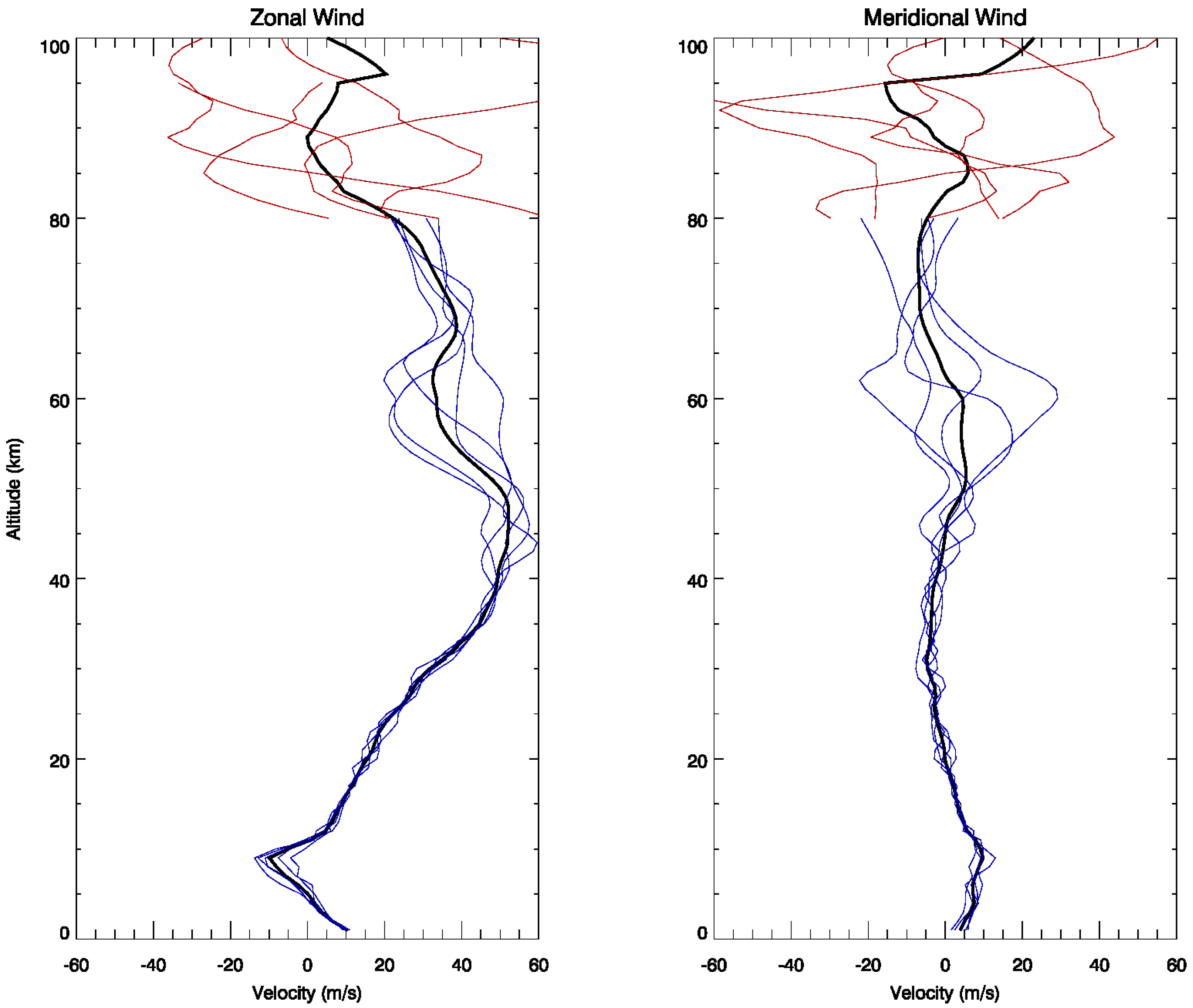
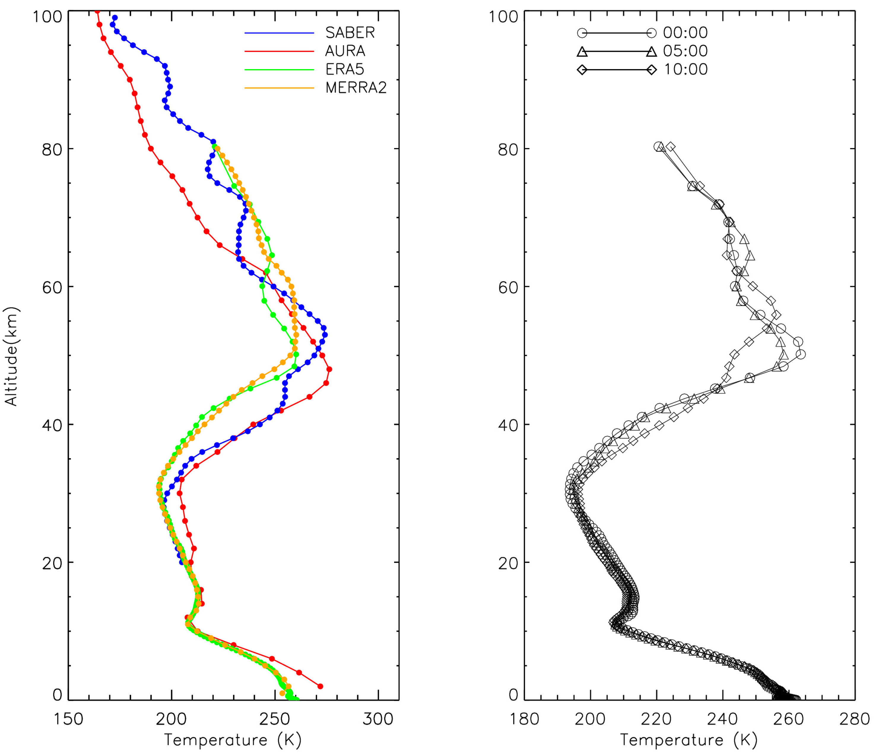
2.2. Meteor Radars and Wind Models

The mesospheric winds used to calculate the intrinsic parameters of gravity wave and analyze the conditions in which the waves propagated were obtained from the meteor radar installed at King Sejong Station (KSS: 62.1° S, 58.7° W). The meteor radar installed at KSS operated at 33.2 MHz with a peak transmitting power of 12 kW. The radar had one transmitting antenna and five receiving antennas, measuring about 23,000 to 35,000 meteor echoes per day [28]. Winds were measured between 80 and 100 km of altitude at every 15 min. In the present work mean winds were averaged within a one-hour interval.

Ferraz Station also hosts a meteor radar (know as “Drake Antarctic Agile MEteor Radar-DrAAMER”) that was installed in March of 2010, but due to a severe fire on the station in February of 2012, the radar operation stopped that year up to 9 March 2020, after a complete rebuilding. The Ferraz radar (DrAAMER) works with eight transmitting antennas, five receiving antennas, a frequency of 36.9 MHz and a peak transmitter power of 30 kW [18].

In addition to the KSS winds, the ERA-5 reanalysis from ECMWF (European Centre for Medium-Range Weather Forecasts) was used to retrieve wind data from 1 to 80 km. Combining the winds of these two data sets we could cover all altitude ranges to conduct the analyses on the gravity wave propagation. Detailed information on the ERA-5 reanalysis are found on Hersbach et al. (2018) [29].

Simultaneous observation of mesospheric winds at KSS and Ferraz station was conducted for the year of 2011 (the only year with good time series of simultaneous data). Wind comparisons were made in order to validate and use KSS wind observations as prevailing winds over Ferraz station. Figure 2 shows one example of wind profiles at 21 UT of 21 June 2011, obtained from the meteor radars operated at Ferraz and KSS (80–100 km), and by ERA-5/ECMWF and MERRA-2/GMAO/NASA reanalysis, and also from the HWM-07 wind model. Reanalysis and model profiles were chosen for the approximate location of Ferraz Station and King Sejong Station (62° S, 58° W), both on King George Island, about 200 km to the north of the tip of the Antarctic Peninsula. The HWM version 2014 was not used in this work because there are no changes in it regarding the parameterizations and any new data input for altitude bellow 100 km in comparison with the version 2007. More information on HWM can be found in Drob et al. (2007 [30]) and Drob et al. (2014 [31]), and details on the MERRA-2 reanalysis are available on Gelaro et al. (2017) [32].

Significant discontinuities were clearly noted between the wind models and the radar measurements, since the winds are from different atmospheric regions, especially in the meridional wind component. For our purposes, the wind profiles were interpolated vertically and averaged using five profiles to avoid significant discontinuity (more details on Section 2.3). Wind profiles obtained from the models show a great difference from each other, except for MERRA-2 and HWM-07 that are quite similar in the zonal wind component. However, MERRA-2 includes more observational data for better accuracy showing variabilities not presented in the HWM profiles. This difference demonstrates some unreliability in using models. For our case, models were the only option of obtaining wind data for higher atmospheric altitudes where no measurements were available, and the accuracy or errors could not be evaluated. Notwithstanding we could not ensure that the ERA-5 wind was the best choice, but it offered satisfactory results, more variability along the profile, higher temporal (1 h), horizontal (31 km) and vertical (137 levels from the surface to 0.01 hPa) resolutions. Besides that, it is the most recent wind model and has not yet been used for similar purposes. Thus it is interesting to evaluate this model for the vertical propagation study of the gravity waves.

Figure 3 shows the monthly averaged winds obtained by ERA-5 and MERRA-2 reanalyses taken at 00:00 UT of April (mid season of Autumn) and July (mid season of Winter) of 2017. Both reanalyses were very similar to each other, and agreements concerning the seasonal variability. The zonal component of the winds from April to July increase in intensity, and the meridional component of the winds changes direction.

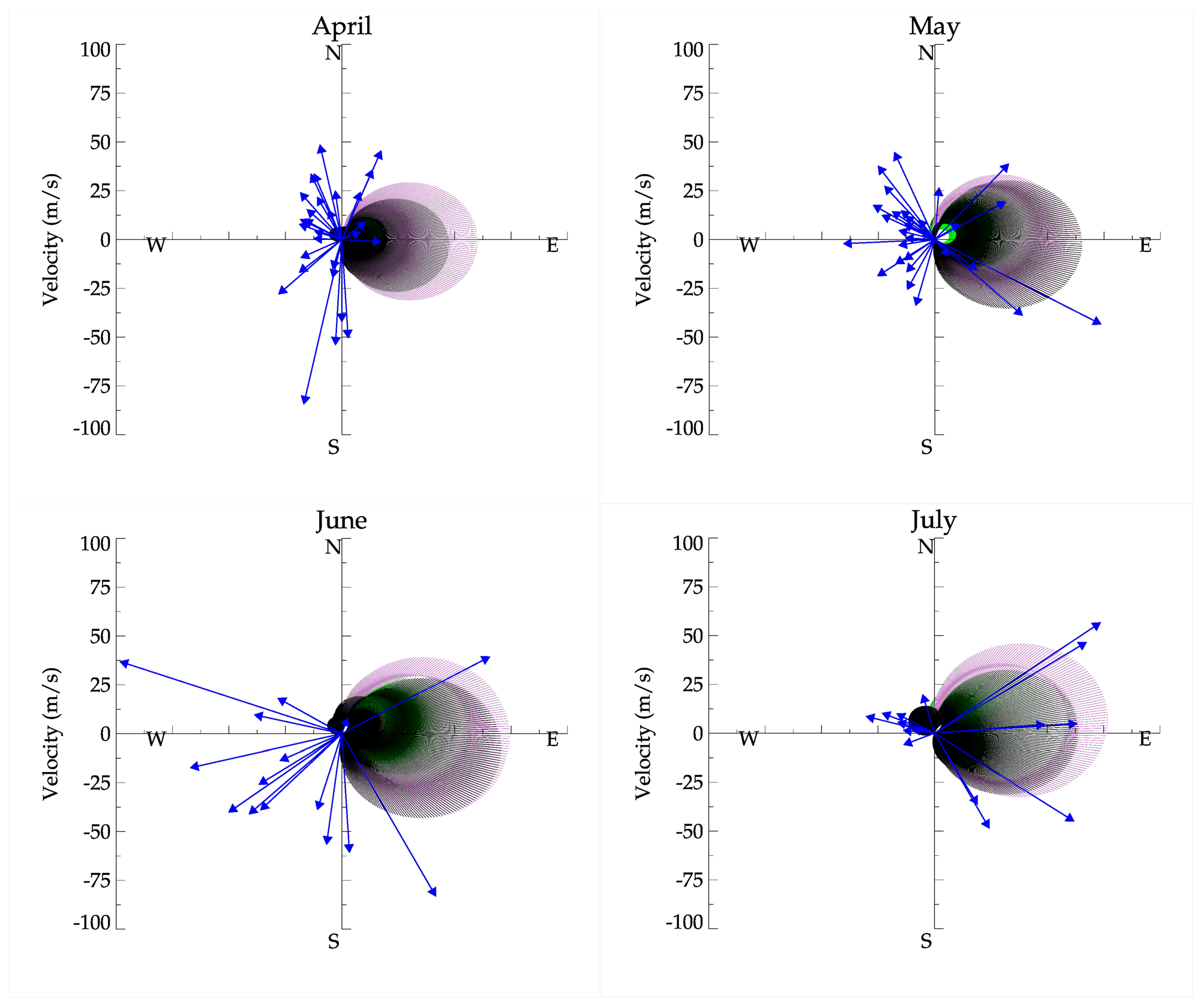
2.3. Blocking Diagram

Blocking diagrams are prepared by following the theory of Gossard and Hooke (1975) [33], which demonstrate the dependency of the wave intrinsic frequency with the background wind. The relation between intrinsic wave frequency ($\widehat{\omega }$) and the background winds ($\overrightarrow{v}$) is given by the following equation:

$$\widehat{\omega }=\overrightarrow{k}·(\overrightarrow{c}-\overrightarrow{v})$$

(1)

where $\overrightarrow{k}$ is the wavenumber vector ($\overrightarrow{k}=(k,l,m)$), and $\overrightarrow{c}$ is the wave phase velocity. As we are interested in the atmospheric region where the intrinsic frequency becomes zero, then Equation (1) can be better represented (knowing that $\overrightarrow{c}=\frac{\omega }{\overrightarrow{k}}$) by:

$$\widehat{\omega }=\omega (1-\frac{v}{c})$$

(2)

It is notable from Equation (2) that the intrinsic frequency $\widehat{\omega }$ goes to zero (and the wave vanishes) when $\overrightarrow{c}$ approaches $\overrightarrow{v}$. Following this approximation, it is possible to infer that the wave is absorbed by the wind if the wave phase speed is less than or equal to the magnitude of the wind in the wave propagation direction.

Horizontal wind (v) can be represented by the zonal ($v_z$) and meridional ($v_m$) wind components as a function of the azimuth ($\varphi$):

$$v=v_z\cos \left(\varphi \right)+v_m\sin \left(\varphi \right)$$

(3)

where the azimuth angle in this equation is defined as degrees counterclockwise from East. Equation (3) represents the wind projected in all directions, and indicates the possible critical levels for vertical gravity wave propagation. Superposition of these critical levels is called blocking diagram [34].

In the present study, blocking diagrams were built using night-time averaged wind profiles provided by ERA-5 reanalysis (1 to ∼80 km) and the KSS meteor radar (80 to ∼100 km). To avoid a discontinuity at 80 km, the wind profiles between 70 and 90 km were interpolated at each 1 km to produce a continuous profile from 1 to 100 km. Then an average wind profile was calculated using five individual profiles from 18:00 UT to 06:00 UT of the next day, and temporally spaced at each 3 h. This time interval was chosen based on the nocturnal airglow observations, and also considering the averaged time of gravity wave propagation from the troposphere to the mesosphere as published in previous works [35,36]. For example, if we set the time of the first wind profile to start about 3 h before the beginning of the airglow observations and the last profile 3 h before the end of the observations, this was quite realistic and could represent well the atmospheric environment.

Figure 4 shows the averaged nocturnal wind profiles as well as the five individual wind profiles from KSS meteor radar and ERA-5 reanalysis for the night of 28–29 April. The black line denotes the averaged profile; the blue line denotes the five individual profiles from ERA-5; the red line denotes the respective five profiles from KSS radar. It can be observed that the averaged nocturnal profile has a great similarity with the individual profiles, and it can represent the general characteristics of the background wind.

The discontinuities at the top of the profile (above 95 km) were due to the lack of some winds from the KSS radar. The mean wind profile shows, in general, that the “night-time” wind was quite smooth and well-represented up to 90 km. Regarding the fact that the waves are visualized in the OH emission layer, near 87 km altitude, and we are interested in the propagation environment below this altitude, the blocking diagrams were constructed from near the ground up to 90 km.

3. Results and Discussions

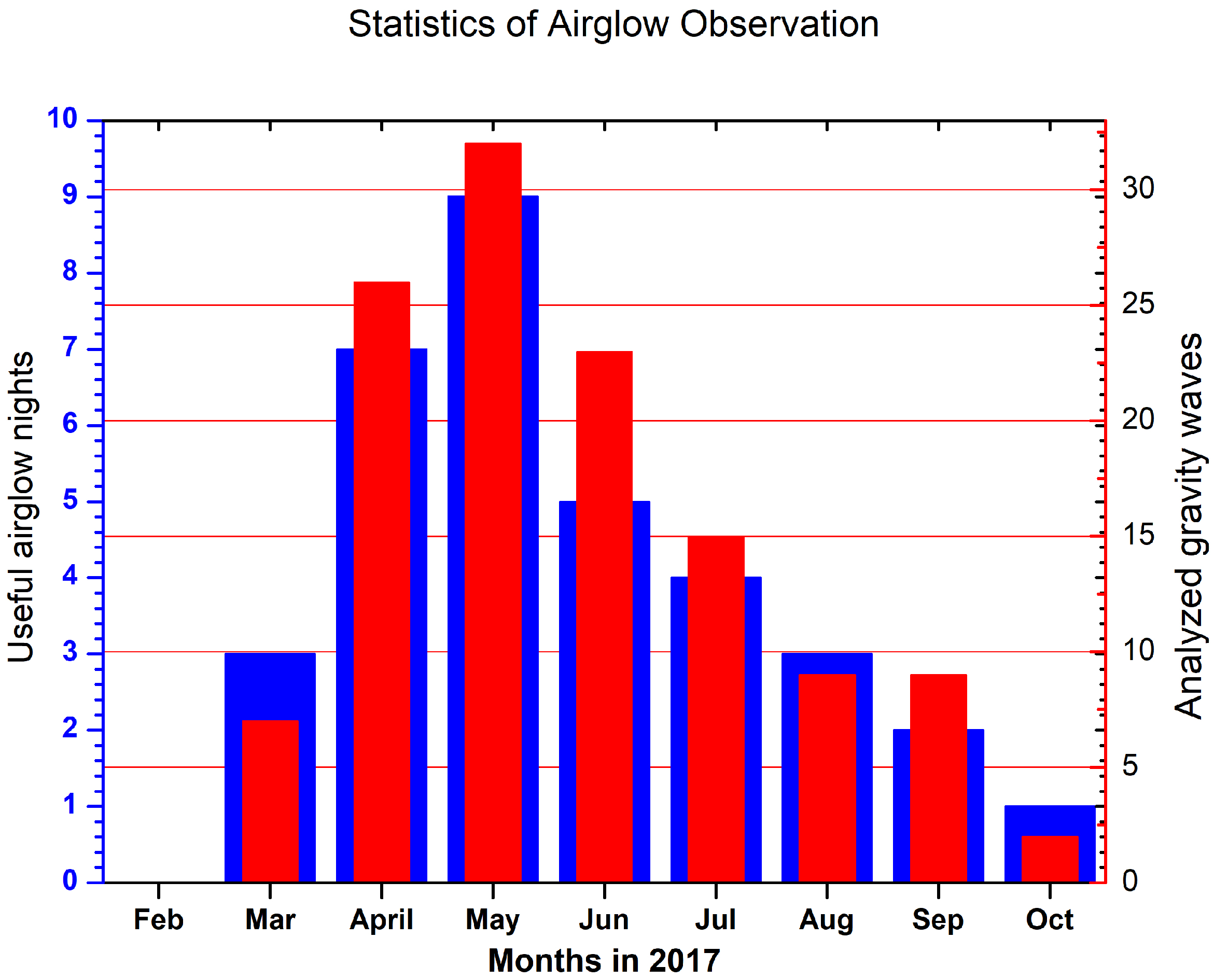
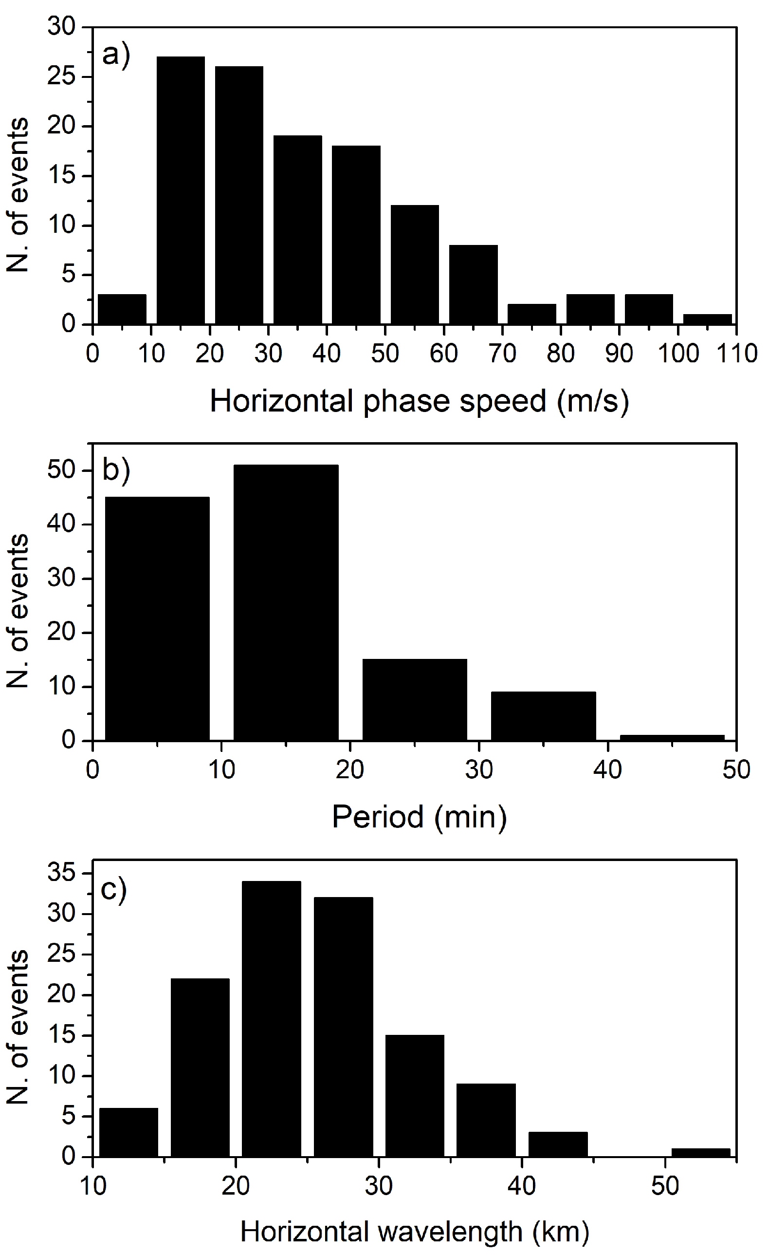
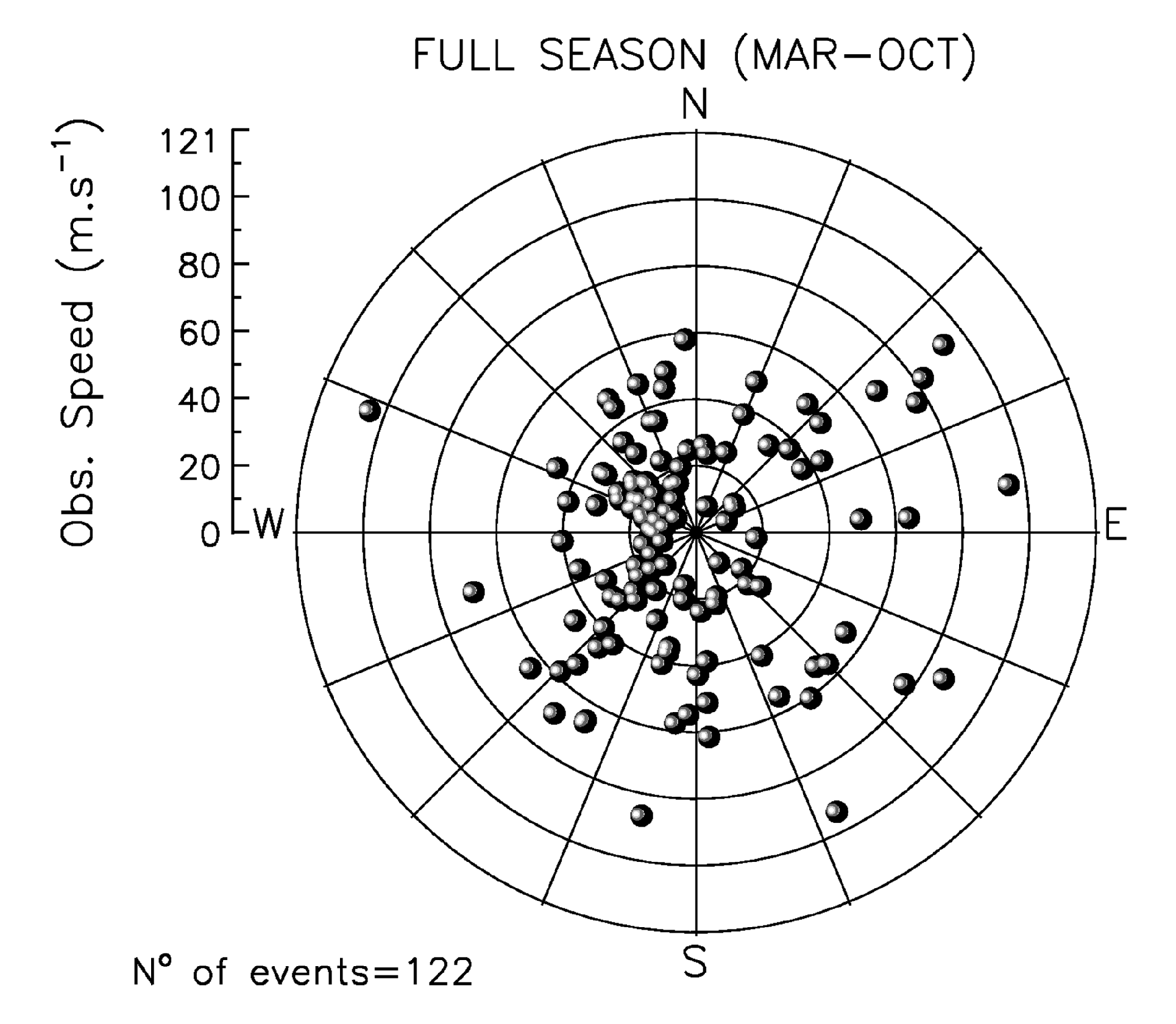
3.1. Airglow Observations

Airglow observations at Ferraz Station are quite limited due to the great number of cloudy nights, associated with bad weather conditions. Thus, one can have around 15 nights per month of observations, based on the New Moon. Figure 5 shows the histograms with the number of nights and gravity wave events analyzed in each month of 2017. It can be seen that the most wave events occurred from April to July, and a total of 122 gravity wave events were observed in 34 nights with at least 2 h of clear sky condition in 2017.

Gravity wave events were analyzed using Fourier spectral analysis (see details on Section 2.1), and classified according to the following physical parameters: horizontal wavelength, observed period and observed phase speed. Figure 6 shows histograms for the number of events regarding their parameters (Table S1 presents all gravity wave parameters in the supplementary material). Gravity wave phase speed (Figure 6A) ranges from 5 to 100 m·s⁻¹, with most of the waves around 10 to 70 m·s⁻¹. The majority of the waves presented observed periods (Figure 6B) from 5 to 15 min (85% of the waves). Regarding the horizontal wavelength, the waves presented wavelengths from a minimum of 10 km up to a maximum of 60 km (just one case with ${\lambda }_h$ > 50 km), with a higher distribution between 20 and 30 km.

Figure 7 shows the distribution of the gravity waves propagation directions, in the polar chart, as a function of the observed phase speed. The distance of each dot from the center of the chart represents the horizontal phase speed, as the angular orientation of the dot is the azimuthal propagation direction of the wave (0° is at North, increasing in the clockwise direction). An anisotropy is observed in the wave propagation direction, with the faster waves (c ≥ 50 m·s⁻¹) propagating mainly to east, south, and southeast directions. However, the majority of the observed waves, including the slower ones, propagated to west and northwest directions.

The resulted anisotropy in the propagation direction of the gravity waves agrees with the results obtained by Bageston et al. [14], at the same site (EACF) in 2007. Other results obtained by airglow imaging near the Antarctic Peninsula, at Halley Station, as described by Nielsen et al. [15] for observations carried out in 2000 and 2001, and recently by Matsuda et al. [6], with data obtained at Halley Station in 2013, also are similar to our results regarding the anisotropy in the gravity wave propagation directions.

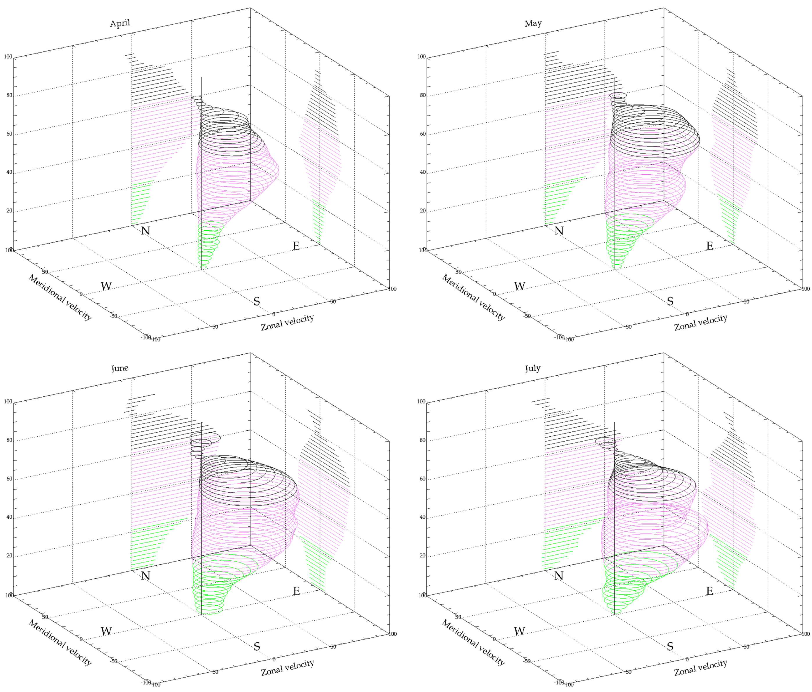
3.2. Blocking Diagrams

The blocking diagram charts were built based on the methodology described in Section 2.3 for April, May, June and July, where the majority (79%) of the gravity waves were observed. The time interval used to calculate the blocking diagrams did not include the entire month, but only a few nights centered on the night of the New Moon. The interval began on the first day with an observed wave in that month and it ended on the last day on which a wave was observed, and it could be in the same month or even at the beginning of the next one, since the time interval was related to the airglow calendar of observations. For example, if there were three or more sequentially nights without wave observations the time interval would end just after the last night. So, the blocking diagram could include up to two nights without wave observations, but not a gap larger than three nights without airglow data.

Figure 8 shows the blocking diagrams for April to July from the ground up to 90 km height. The time interval considered to represent the April airglow observations started on April 22 and finished on May 2 early morning. This interval contained 28 gravity waves observed during 10 relatively clear nights. Thus, blocking diagram charts for April were prepared with an average wind based on 10 nights, where each of these nights contained five wind profiles 3 hours apart from one another, as described in Section 2.3 and Figure 4. For May, the blocking diagram included wind profiles from May 23 until the early morning of June 2, with 10 sequential nights and containing 29 gravity wave events. The used sequential nights of June comprise the period from June 23 to 27, with four nights on which 15 wave events were observed. Finally, in July the nights from 16th to 22nd were used, with six nights and 17 observed gravity waves.

Blocking regions from 2 km to 20 km are in green lines, corresponding to the characteristic winds of troposphere region mainly, and including the lower stratospheric portion; blocking regions between 21 and 60 km are in purple and corresponds approximately to the stratosphere region; in black (upper portion) are the blocking regions for the mesosphere (including the OH airglow layer and the mesopause), that comprises the region from 60 km to 90 km. From Figure 8 one can see that blocking regions in the troposphere intensified from May to July, but in all months were quite small. In the stratosphere and lower mesosphere the blocking regions were larger than in the troposphere, and it is possible to observe significant changes in the shape and size (more changeable than the tropospheric blocking layers) between the different months. For the mesosphere, we observed a significant change of directions in the blocking regions above 80 km height in each month. In addition, the wind intensity near the mesopause (∼85–90 km) was much stronger in June than in April and May.

For a better understanding of the impact of the wind in the wave filtering, the blocking diagrams are plotted in a polar chart, along with the gravity waves phase speed drawn as an arrow (vector) from the origin to the respective point in order to represent, simultaneously, the wave direction and velocity. That way, Figure 9 shows the horizontal phase speed vectors of the waves along with the blocking diagrams from Figure 8. The colors of the blocking regions correspond to the same colors used in the Figure 8. The blocking diagram in a polar chart indicates a high correspondence between the preferable propagation direction of the observed waves and the mean wind in the regions below the observation layer (∼87 km). Then, it is clearly seen that most of the vectors do not lie within the blocking regions.

Throughout the months most of the gravity waves were outside the blocking regions, mainly because the majority of the waves were not oriented to the east (dominant blocking region). For those 14 gravity waves inside the blocking region in May and July, many of them were fast and also escape the blocking regions. The east represented the preferential blocking regions in almost all atmospheric layers. In April only three waves were propagating to the east and were inside the mesospheric blocking region, and as they had a very small phase speed probably had in situ generation. Similar situations occurred in May and June, with relatively slow waves inside the mesospheric blocking region. These waves could be generated by wave breaking or recombination of waves by wave–wave interactions, similarly to those studied by Taylor and Hapgood, and Hecht [37,38].

In June, the tropospheric blocking region moved and spread to the east and northeast, but no gravity waves were observed inside this blocking region. In July, two relatively fast waves propagating to the east were seen blocked in the stratosphere region. Potentially, these two waves could have been generated in the stratosphere, or they could come from long distances (from the west) ducted in the mesosphere, or stratosphere heights. The wave ducting over long distances was studied by Walterscheid et al. [39], and other studies about energy transports by ducted waves were conducted by Hecht et al. [40]. In July, it was also observed one wave (the smaller vector) propagating to the northwest that was trapped in the mesospheric blocking region.

Similar general wave filtering results were found by Perwitasari et al. [41] in 2013, using an M-transform applied to airglow data from Syowa Station (69° S, 40° E). They found a westward preferable propagation direction, supposedly due to filtering by winds eastward oriented in almost all atmospheric layers, analogous to our blocking diagrams.

June was the month that better represented the wave filtering. With only one exception (a wave with a low phase speed and trapped in the blocking region in mesosphere), all waves escaped the blocking diagram region either due to their speed or to their direction. This blocking diagram was built by an average of four nights, and it was the one that better represented the typical environment where the waves propagated.

No blocking diagrams showed wave events trapped in the tropospheric blocking region, and this suggests that most of the observed waves were blocked mainly in the stratospheric region. However, this result does not indicate a possible source region and such waves could be generated both in the troposphere as well as above that region.

The blocking diagrams presented in Figure 9 show a considerable number (11%) of waves trapped in the mesospheric region. These gravity waves were generally oriented to the east and had slow velocity in April, May and June, but the waves were relatively fast in July. These facts could be explained by wave ducting and the high winds variability above 80 km (see the upper part of the diagrams showed in Figure 8 and also at the top of Figure 4). This variability could be explained by atmospheric tides and also due to wave breaking, including the gravity waves and waves of other scales that are not identified in the airglow images. The next section includes a short discussion of the tidal influence in the nocturnal averaged wind.

There seemed to be a direct relationship between the wind filtering (waves propagating out to the blocking region), represented by the blocking diagrams, and the number of nights used to build the blocking diagrams. When a larger number of days (or full nights) were used on the average blocking diagram, more waves were inside the blocking regions. Blocking diagram analysis performed over a short time interval (only during the useful airglow nights) can be very useful for the Antarctica Peninsula, since the number of airglow observations on that region is concentrated in short periods (and also sparse). This region is different from other sites, such as mid-low latitudes, where the waves can be observed during several consecutive nights and blocking diagrams can be constructed based on monthly or seasonal mean winds [34,42,43,44].

Tomikawa (2015) [45] developed a theoretical study where the blocking diagrams can represent both the critical levels and turning levels, and consequently better represents waves filtering. The turning levels are represented by a layer with squared vertical wavelength equals to zero ($m^2=0$), where a wave would be reflected. This kind of diagram was so-called transmitting diagrams because they represent both the critical level filtering and the turning level reflection. The turning levels consider the horizontal wavelength and the Brunt–Vaisälä frequency, and once we have the observation of these parameters from an airglow CCD camera and temperature from satellite, the above theoretical study could be applied for future works with the goal of better representing the waves preferential propagation directions.

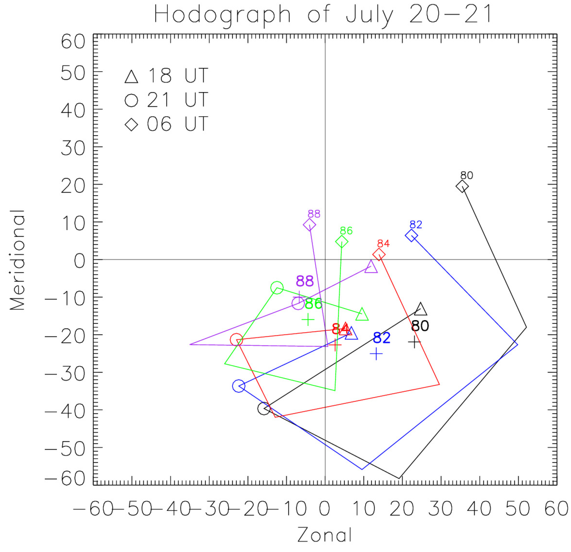
4. Case Study of July 20–21

This section presents the analyses for one interesting night in which it was observed a large number of gravity waves. This special night was July 20–21 and comprised more than 13 h of clear sky conditions, ranging from 21:00 UT (18:00 LT) to 10:40 UT (07:40 LT). During this clear sky night, it was possible to identify eight small-scale waves and one medium-scale gravity wave that were fully characterized.

This case study was conducted because it was a very characteristic observation night at EACF, containing a variety of waves (small-scale, including bands and ripples, and one case of medium-scale wave). This case study includes mainly an analysis of a blocking diagram and the application of a reverse ray tracing model for all gravity waves observed in this night.

Table 1. Characteristics of gravity waves observed on the night of July 20–21.

Wave #	Observed	Horizontal	Period	Phase	Propagation
	Time (UT)	Wavelength (km)	(min)	Speed (m/s)	Direction (°)
1	21:49	23.2	7.9	49.2	84.8 (E)
2	22:07	26.3	24.9	19.6	301.0 (NW)
3	02:55	26.8	31.9	14;0	276.0 (W)
4	03:11	52.0	34.0	25.5	294.0 (NW)
5	03:23	15.6	14.9	17.4	289.5 (W)
6	05:48	29.3	32.6	15.0	246.4 (W)
7	08:29	39.3	10.3	63.5	85.6 (E)
8 ${}^{+}$	08:30	181.0	30.0	99.0	98.8 (E)
9	10:32	37.6	8.2	76.7	126 (SE)

${}^{+}$ Medium-scale wave.

presents the characteristics of all observed gravity waves on July 20–21. The waves were labeled by numbers and listed according to their respective observation time. The medium-scale wave event was not included in the statistics presented in Figure 6 and Figure 7, but is included in this case study. This event was analyzed by using the keogram technique (similar spectral analysis methodology employed by Figueiredo et al. [46] on keograms of the perturbed total electron content).

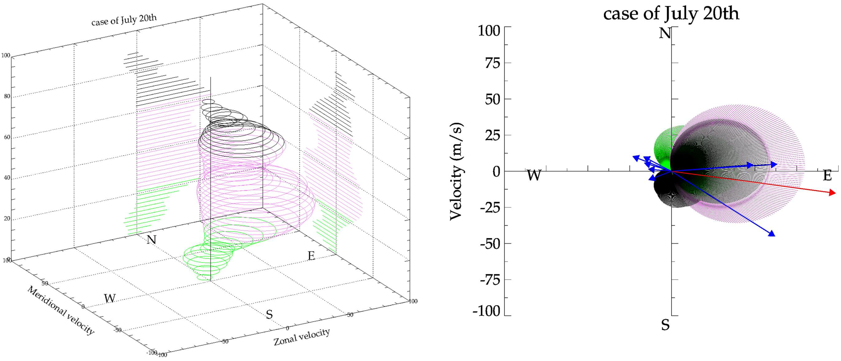
4.1. Blocking Diagram Analysis

The blocking diagram for this case study was prepared in a similar way to the previous cases (months), here with usage of the nocturnal mean winds, calculated with the wind profiles from 18 UT up to 06 UT, separated at every 3 h. The blocking diagram and its projection in a polar chart along with the wave phase speed vectors are shown in Figure 10. In the polar chart, the blue arrows represent the small-scale waves and the red arrow represents the medium-scale wave event.

From Figure 10 it is possible to recognize the typical behavior of waves observed in the winter season, that is, faster waves propagating to the east and southeast, while the slower waves propagated to northwest and west directions. Small-scale waves propagating to the west were out of the blocking regions, as well as the fast small-scale wave propagating southeastward and the medium-scale wave propagating eastward. It can be seen that two small-scale waves propagated eastward and these waves were trapped in the blocking region corresponding to the mesospheric winds. Supposedly these waves propagated in some kind of duct, or they were generated locally in the upper mesosphere by wave breaking or wind shear.

The diagram on the right panel of Figure 10 shows good results when we compare the wave filtering with the typical wave propagation directions on that night. As the nocturnal averaged wind was used for constructing this blocking diagram, we can assume that this wind well represents the environment where the waves were propagating. We suggest making use of this methodology when only one or a few observation nights are available, even knowing that some errors can still occur due to large winds variability in the region above 80 km height.

In order to analyze the influence of atmospheric solar tides in the nocturnal averaged wind, a hodograph was constructed for the night of July 20–21 based on winds obtained by the KSS meteor radar from 18 to 06 UT (five profiles) at five altitude levels, from 80 to 88 km, each spaced at 2 km intervals. The hodograph is presented in Figure 11 where each line represents the wind direction and intensity at different altitudes, showing a clear variability throughout the night. Triangles indicate the wind at the initial time (18 UT), circles indicate the wind at 21 UT, and squares indicate the wind at the last used time (06 UT). Crosses indicate the average wind associated with each altitude level (five-colored curves), and the altitude levels are labeled just above the crosses.

The hodograph shows that the turn of the wind was counterclockwise for all the considered altitudes (80, 82, ..., 88 km), mainly due to the semi-diurnal tide component (12-h global oscillation) which was the dominant tidal component at Ferraz. The value of the average wind in the nocturnal period interval (crosses) represents the winds with an amplitude smaller due to averaging the wind variations in the nocturnal period. Subtracting a part of the wind variability justified the small wind values in the blocking regions above 80 km. Although the nocturnal averaged wind profile did not represent a “true” wind at the wave observation instant, it could be a good approximation for a background wind, and it was useful for blocking diagrams.

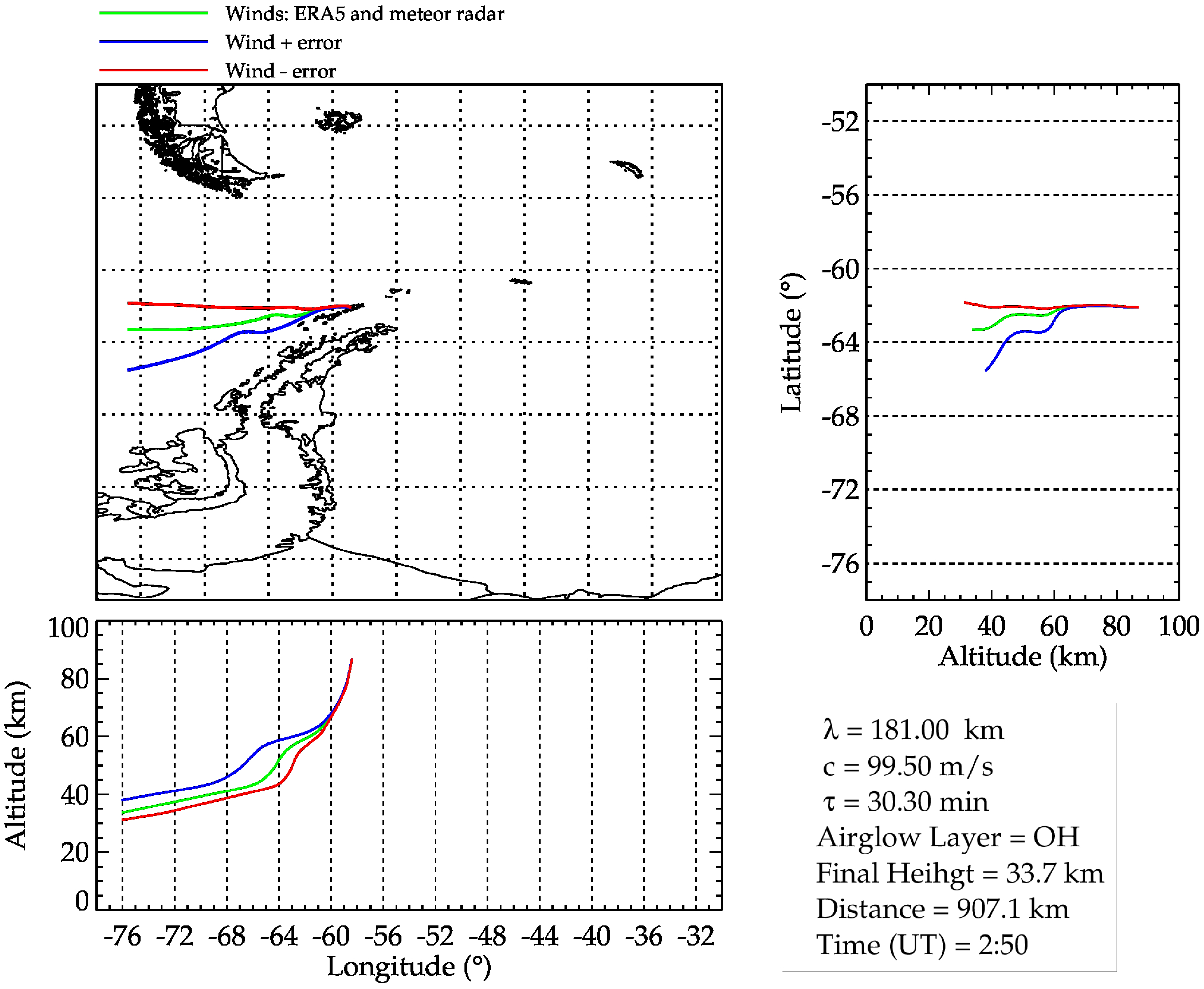
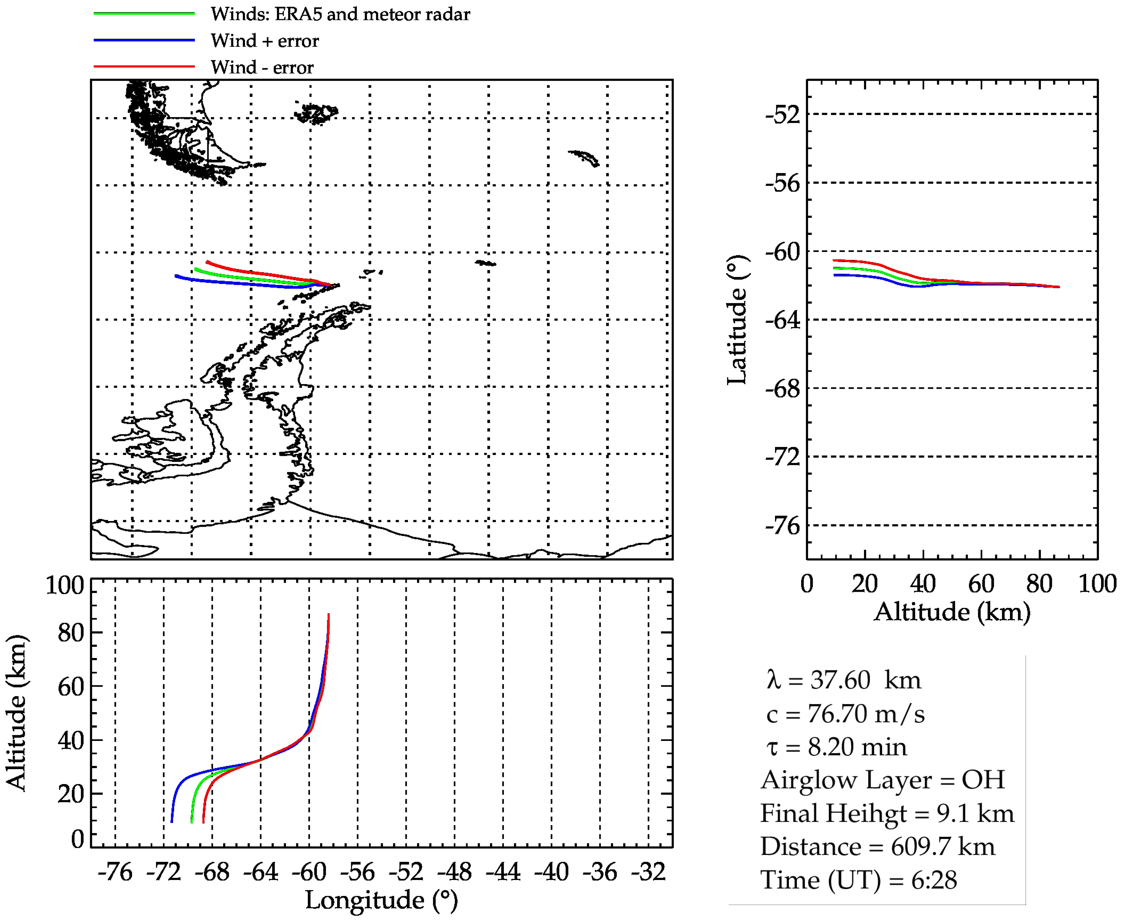
4.2. Reverse Ray Tracing

A reverse ray tracing model was used to estimate the most likely gravity wave source for the waves observed in July 20–21. The model used in this paper is the same developed by Wrasse et al. (2006) [35]. It is based mostly on the position and refraction equations of a wave packet , described by Lighthill (1978) [47], and employs the group velocities and dispersion relations described by Marks and Eckermann (1995) [48].

The time step is determined using the relation between the value of the vertical group velocity and a height decrement of 100 m ($\delta t=\frac{\delta z}{c_{gz}}$). The model has four stopping conditions, which were checked after each height step, as follows: the vertical wave number squared must remain positive; intrinsic frequency must continue positive, unless the wave is filtered; if the vertical wave number squared takes a value above ${10}^{-6}$, the wave is close to a critical level, and the model must stop; and altitude of the wave must be positive, indicating the wave have not reached the ground. The stopping conditions and time-step method are discussed in Wrasse et al. (2006) [35].

The model required a data set of hourly winds and temperature for 00:00 UT of the day of observation to 12:00 UT of the next day, from 0 to 95 km of altitude. The used data set was composed of interpolated winds of ERA-5 and KSS meteor radar. Ray tracing also needs the input of temperature and Brunt–Väisälä frequency ($N^2$, which is derived from the temperature), and that data set was obtained from the Microwave Limb Sounder (MLS) instrument aboard AURA satellite, that passed near EACF at 19:00 UT on July 20 and at 04:38 UT on July 21, measuring temperature from the ground up to 100 km height (from 1000 hPa to ${10}^{-5}$ hPa, pressure levels). The temperature profile obtained at 19:00 UT was reproduced for 12:00 UT to 21:00 UT, and the profile of 05:00 UT was reproduced for 22:00 UT to 12:00 UT of July 21.

Regarding the winds used as input in the ray tracing, it was constructed by using two other wind data sets with shifted (to left and to right) values from the standard (original) wind profiles to represent the associated error. One data set was prepared by adding the error to the standard wind, and for the other wind data, the error was subtracted from the original wind. For altitudes above 80 km, the available radar errors are used for each altitude of wind measurements. A generic error is evaluated by taking the difference between the ERA-5 and HWM-07 winds and dividing the result by two, as shown in the following equation.

$$\sigma =\frac{|ERA5-HWM|}{2}$$

(4)

The result obtained by Equation (4) (σ) is used as an estimation of error values to build two new wind data set from the ground up to 80 km. With these new data sets, it is possible to infer how a small wind variability (winds shifted from the original values) can have an influence on the ray tracing paths and in the initial values of the intrinsic frequency. Although this methodology does not retrieve a real error (uncertainty), it can represent a certain deviation from a base value using other models as parameters.

Figure 12 shows temperature profiles for the night of July 20–21. Measurements from TIMED/SABER sounding (blue profile) on that night at 02:14 UT (at a distance of ∼500 km from EACF); the sounding of AURA/MLS (red) at 04:38 UT (about 300 km from station); MERRA-2 (orange) and ERA-5 (green) temperature profiles for 04:00 UT. In addition, Figure 12 shows (right panel) three individual temperature profiles from ERA-5 at 00:00, 06:00, 10:00 UT showing small variability of the temperature profiles along a time interval of 10 h.

Quantitative results obtained from the reverse ray tracing applied to the waves listed in Table 1 are summarized in

Table 2. Wave path results obtained by the reverse ray tracing model to each wave listed in Table 1.

Wave #	Observed	Generated	Final Height	Horizontal	Propagating	Direction
	Time (UT)	Time (UT)	(km)	Distance (km)	Direction (°)	Stopped
1	21:49	20:11	72.3	129.6	84.8 (E)	W
2	22:07	21:23	86.9	30.6	301.0 (NW)	E
3	02:55	02:11	83.2	136	276.0 (W)	-
4	03:11	2:52	84.4	33.9	294.0 (NW)	-
5 ${}^{*}$	03:23	-	-	-	289.5 (W)	-
6	05:48	03:54	4.3	118.8	246.4 (W)	SW
7	08:29	05:16	63.6	397.4	85.6 (E)	SW
8 ${}^{+}$	08:30	02:50	33.7	907.1	98.8 (E)	W
9	10:32	06:28	9.1	609.7	126 (SE)	W

${}^{*}$ Ray tracing stopped at the second iteration. ${}^{+}$ Medium scale wave.

, and the waves were enumerated by following their observation time. The ray tracing results indicated that only two waves were generated at the troposphere (below 10 km), one event at the stratosphere (between 10 and 60 km), and the other 6 events were likely generated in the mesosphere (above 60 km). Most waves propagated from close locations (considering a horizontal straight line) of the Ferraz station. Results provided by the wind shifted from the original wind profiles showed to be quite similar to the standard one for most cases.

Results for the ray tracing paths of the gravity waves # 2 to # 5 shows that these waves were potentially generated in the upper mesosphere (near the OH airglow layer), i.e., between 80 and 90 km height, and it was noted that the model stopped just after a few iterations. The error analysis showed that the distance in which the waves # 2 and # 3 propagated above 80 were longer for a smaller deviated wind than when the standard wind was used.

Waves # 1 and # 7 had a similar propagation direction inside the blocking region, were generated in the lower mesosphere (∼60 to 70 km). These cases were potentially generated due to a wind shear near the stratopause, that propagated vertically and horizontally a few kilometers and reached the OH airglow layer. In addition, these results confirm the initial hypothesis that they were generated above the blocking region. These two cases also could be originated by the effect of a primary wave breaking at some critical level around 60 km, which generated a secondary wave that propagates up to the observed airglow layer. Trinh et al. 2018 [49] demonstrated the Antarctic Peninsula as a hot-spot of secondary wave generation after wave breaking (from 30 to 90 km), using satellite data in the austral winters of 2010–2013. Other studies, like the ones conducted by Vadas et al. 2013, 2014 [50,51] have used modeling to investigate the propagation of secondary waves generated after wave breaking. Ray paths resulted from the shifted wind profile showed very similar results comparing to the standard winds, allowing the waves to propagate to a similar altitude and also to a close region of the station for all paths.

Ray paths of the medium-scale gravity wave (wave # 8) are shown in Figure 13. The first panel (top-left) shows the horizontal propagation of the wave paths over the map showing the tip of South America and the Antarctic Peninsula region. Green path represents the wave path calculated with the standard interpolated wind data set (ERA and meteor radar), while the blue and red paths represent the paths obtained, respectively, by the positive and negative shifted winds. The second panel at the bottom shows the wave paths as a function of longitudes and altitudes, and finally, the right panel shows the wave paths in a latitudes versus altitudes frame.

At the right-bottom corner of Figure 13 the parameters of the analyzed wave are shown along with the numeric results of the ray tracing: final height (altitude where the ray path stopped); Distance (in a straight line from the observatory to the ray path stopped position); time (UT time of the wave origin). Wave # 8 traveled a great distance horizontally to the west, but the ray tracing stopped because the wave reached the limit of the used longitude grid. This result is quite inconclusive since the wave probably was generated far away (maybe more than one thousand kilometers) to the west of the station, justified by the large horizontal speed of the wave (∼100 m·s⁻¹). The deviated (shifted) wind made the paths spread some degrees in longitude and latitude, but in the three cases, the wave propagated in a similar direction.

Ray paths for wave # 9 are shown in Figure 14, in the same way as Figure 13. Wave # 9 is the fastest (76.7 m·s⁻¹) small-scale gravity wave event with a relatively large structure (for small-scale waves) that propagated for hundreds of kilometers from the troposphere to the OH airglow emission height. Ray paths for the deviated wind profile showed that Wave # 9 came from a close region. Waves # 6, # 8, and # 9 confirm the results obtained from the blocking diagram, as they are faster than the wind and could propagate from the lower atmosphere to the mesosphere without any filtering process or reflection caused by the wind.

Reverse ray tracing results obtained by Rourke et al. [52] using OH airglow radiometer images observed at Davis Station showed very similar results to the present study, with a large number of ray paths stopped around the airglow layer. The authors also found that only 15% of the gravity wave ray paths originated in the troposphere, and a few cases in the stratosphere.

For waves # 6 and # 9, where the ray tracing indicates sources in the troposphere, no meteorological phenomena could be associated with them. However, they should be generated by some physical disturbance process in those altitudes, such as wind shear or temperature inversion layers, that are not easily identified with satellite images or reanalysis of meteorological fields. Although the estimation of the wave sources was quite inconclusive and complicated to indicate a specific source, the ray paths showed expected results regarding the blocking diagrams results.

The data set prepared with vertical interpolation in the winds was provided by two distinct methods: one observed by radar in the altitude range from 80 to 100 km; other obtained from reanalysis produced at pressure levels (corresponding to altitudes ranging from ∼1 km up to 80 km height), showed consistent results in the estimation of the gravity waves paths and the wave filtering. An error estimation in the interpolated winds verified the importance of the wind in the wave dynamics and source estimation, for the Antarctic Peninsula region, although an ideal data set is not available.

5. Conclusions

The present study showed the observed gravity wave characteristics, the analysis of wave propagation as a function of the wind filtering for the year of 2017 over Comandante Ferraz Antarctic Station (EACF). In addition, a case study for one night of high activity of gravity waves was conducted, using blocking diagrams and ray tracing model to identify the locations (regarding altitude and distance from the observatory) of the origin of the waves. An FFT spectral analysis was applied to 122 gravity wave events, distributed along 34 nights with clear sky conditions. The typical parameter values of the analyzed waves were: observed horizontal phase speed around 10 to 70 m·s⁻¹; observed periods typically in an interval from 5 to 20 min; horizontal wavelength mainly between 15 and 35 km; the majority of the waves propagates to the northwest and west directions, with small phase speed; and the faster events propagate to east and south directions.

Blocking diagrams were built to analyze the wave filtering conditions for the months of April, May, June and July. The nocturnal averaged wind profiles were used to prepare the blocking diagrams, and demonstrated to be appropriate for this purpose. Blocking diagrams with fewer nights demonstrated a better accuracy than the ones constructed over longer time periods. The results from the blocking diagrams showed an anisotropy in the wave propagation direction in agreement to the observed horizontal propagation directions. It is suggested that for future studies averages of wind be used in short days interval for hard airglow observational conditions and hourly winds be used for analyses of specific wave filtering.

A case study on the night of July 20–21 was conducted by analyzing a one-night blocking diagram and applying a reverse ray tracing model to nine observed gravity waves. The ray paths indicated that: (1) six among eight small-scale gravity waves were generated in the mesosphere region (two of them around the mesopause); (2) only two small-scale waves were potentially generated in the troposphere (none of these two waves were linked to any clear meteorological source); (3) the ray path for the medium-scale wave stopped more than 600 km to the west of the station (at around 33 km of altitude), due to reaching the limit of the used data grid (in lat./lon.), and it was potentially generated far away (>1000 km) from the observatory in the lower stratosphere or troposphere. Despite the fact that none of the waves could be associated with any reliable source, the ray tracing confirmed the general results obtained by the blocking diagrams and further investigations (with a larger set of wave events in distinct seasons) should be conducted in future works.

References

1. Nappo, C. An Introduction to Atmospheric Gravity Waves; International Geophysics; Elsevier Science: San Diego, CA, USA, 2002. [Google Scholar]
2. Holton, J.R.; Alexander, M.J. The Role of Waves in the Transport Circulation of the Middle Atmosphere. In Atmospheric Science Across the Stratopause; American Geophysical Union (AGU): Washington, DC, USA, 2013; pp. 21–35. [Google Scholar] [CrossRef]
3. Fritts, D.C.; Alexander, M.J. Gravity wave dynamics and effects in the middle atmosphere. Rev. Geophys. 2003, 41. [Google Scholar] [CrossRef] [Green Version]
4. Krisch, I.; Preusse, P.; Ungermann, J.; Dörnbrack, A.; Eckermann, S.D.; Ern, M.; Friedl-Vallon, F.; Kaufmann, M.; Oelhaf, H.; Rapp, M.; et al. First tomographic observations of gravity waves by the infrared limb imager GLORIA. Atmos. Chem. Phys. 2017, 17, 14937–14953. [Google Scholar] [CrossRef] [Green Version]
5. Pautet, P.D.; Taylor, M.J.; Eckermann, S.D.; Criddle, N. Regional Distribution of Mesospheric Small-Scale Gravity Waves During DEEPWAVE. J. Geophys. Res. Atmos. 2019, 124, 7069–7081. [Google Scholar] [CrossRef] [Green Version]
6. Matsuda, T.S.; Nakamura, T.; Ejiri, M.K.; Tsutsumi, M.; Tomikawa, Y.; Taylor, M.J.; Zhao, Y.; Pautet, P.D.; Murphy, D.J.; Moffat-Griffin, T. Characteristics of mesospheric gravity waves over Antarctica observed by Antarctic Gravity Wave Instrument Network imagers using 3-D spectral analyses. J. Geophys. Res. Atmos. 2017, 122, 8969–8981. [Google Scholar] [CrossRef]
7. Suzuki, S.; Shiokawa, K.; Otsuka, Y.; Ogawa, T.; Nakamura, K.; Nakamura, T. A concentric gravity wave structure in the mesospheric airglow images. J. Geophys. Res. Atmos. 2007, 112. [Google Scholar] [CrossRef] [Green Version]
8. Lai, C.; Yue, J.; Xu, J.; Straka, W.C.; Miller, S.D.; Liu, X. Suomi NPP VIIRS/DNB imagery of nightglow gravity waves from various sources over China. Adv. Space Res. 2017, 59, 1951–1961. [Google Scholar] [CrossRef]
9. Demissie, T.D.; Espy, P.J.; Kleinknecht, N.H.; Hatlen, M.; Kaifler, N.; Baumgarten, G. Characteristics and sources of gravity waves observed in noctilucent cloud over Norway. Atmos. Chem. Phys. 2014, 14, 12133–12142. [Google Scholar] [CrossRef]
10. Kim, Y.; Eckermann, S.D.; Chun, H. An overview of the past, present and future of gravity-wave drag parametrization for numerical climate and weather prediction models. Atmos. -Ocean 2003, 41, 65–98. [Google Scholar] [CrossRef]
11. Medvedev, A.S.; Yiğit, E. Gravity Waves in Planetary Atmospheres: Their Effects and Parameterization in Global Circulation Models. Atmosphere 2019, 10, 531. [Google Scholar] [CrossRef] [Green Version]
12. Xu, X.; Xue, M.; Teixeira, M.A.C.; Tang, J.; Wang, Y. Parameterization of Directional Absorption of Orographic Gravity Waves and Its Impact on the Atmospheric General Circulation Simulated by the Weather Research and Forecasting Model. J. Atmos. Sci. 2019, 76, 3435–3453. [Google Scholar] [CrossRef]
13. Hindley, N.P.; Wright, C.J.; Smith, N.D.; Mitchell, N.J. The southern stratospheric gravity wave hot spot: Individual waves and their momentum fluxes measured by COSMIC GPS-RO. Atmos. Chem. Phys. 2015, 15, 7797–7818. [Google Scholar] [CrossRef] [Green Version]
14. Bageston, J.V.; Wrasse, C.M.; Gobbi, D.; Takahashi, H.; Souza, P.B. Observation of mesospheric gravity waves at Comandante Ferraz Antarctica Station (62° S). Ann. Geophys. 2009, 27, 2593–2598. [Google Scholar] [CrossRef]
15. Nielsen, K.; Taylor, M.; Hibbins, R.; Jarvis, M. Climatology of short-period mesospheric gravity waves over Halley, Antarctica (76° S, 27° W). J. Atmos. Sol. -Terr. Phys. 2009, 71, 991–1000. [Google Scholar] [CrossRef]
16. Moffat-Griffin, T.; Hibbins, R.E.; Jarvis, M.J.; Colwell, S.R. Seasonal variations of gravity wave activity in the lower stratosphere over an Antarctic Peninsula station. J. Geophys. Res. Atmos. 2011, 116. [Google Scholar] [CrossRef] [Green Version]
17. de la Torre, A.; Alexander, P.; Hierro, R.; Llamedo, P.; Rolla, A.; Schmidt, T.; Wickert, J. Large-amplitude gravity waves above the southern Andes, the Drake Passage, and the Antarctic Peninsula. J. Geophys. Res. Atmos. 2012, 117. [Google Scholar] [CrossRef] [Green Version]
18. Fritts, D.C.; Janches, D.; Iimura, H.; Hocking, W.K.; Bageston, J.V.; Leme, N.M.P. Drake Antarctic Agile Meteor Radar first results: Configuration and comparison of mean and tidal wind and gravity wave momentum flux measurements with Southern Argentina Agile Meteor Radar. J. Geophys. Res. Atmos. 2012, 117. [Google Scholar] [CrossRef] [Green Version]
19. Baumgarten, K.; Gerding, M.; Baumgarten, G.; Lübken, F.J. Temporal variability of tidal and gravity waves during a record long 10-day continuous lidar sounding. Atmos. Chem. Phys. 2018, 18, 371–384. [Google Scholar] [CrossRef] [Green Version]
20. Beldon, C.L.; Mitchell, N.J. Gravity wave–tidal interactions in the mesosphere and lower thermosphere over Rothera, Antarctica (68° S, 68° W). J. Geophys. Res. Atmos. 2010, 115. [Google Scholar] [CrossRef]
21. Suzuki, S.; Nakamura, T.; Ejiri, M.K.; Tsutsumi, M.; Shiokawa, K.; Kawahara, T.D. Simultaneous airglow, lidar, and radar measurements of mesospheric gravity waves over Japan. J. Geophys. Res. Atmos. 2010, 115. [Google Scholar] [CrossRef]
22. Vincent, R.A.; Kovalam, S.; Reid, I.M.; Younger, J.P. Gravity wave flux retrievals using meteor radars. Geophys. Res. Lett. 2010, 37. [Google Scholar] [CrossRef]
23. Nyassor, P.K.; Buriti, R.A.; Paulino, I.; Medeiros, A.F.; Takahashi, H.; Wrasse, C.M.; Gobbi, D. Determination of gravity wave parameters in the airglow combining photometer and imager data. Ann. Geophys. 2018, 36, 705–715. [Google Scholar] [CrossRef]
24. Garcia, F.J.; Taylor, M.J.; Kelley, M.C. Two-dimensional spectral analysis of mesospheric airglow image data. Appl. Opt. 1997, 36, 7374–7385. [Google Scholar] [CrossRef] [PubMed] [Green Version]
25. Bageston, J.V.; Wrasse, C.M.; Batista, P.P.; Hibbins, R.E.; C Fritts, D.; Gobbi, D.; Andrioli, V.F. Observation of a mesospheric front in a thermal-doppler duct over King George Island, Antarctica. Atmos. Chem. Phys. 2011, 11, 12137–12147. [Google Scholar] [CrossRef] [Green Version]
26. Wrasse, C.M.; Takahashi, H.; de Medeiros, A.F.; e Michael John Taylor, L.M.L.; Gobbi, D.; Fechine, J. Determinação dos parâmetros de ondas de gravidade através da análise espectral de imagens de aeroluminescência. Braz. J. Geophys. 2007, 25. [Google Scholar] [CrossRef] [Green Version]
27. Bevington, P.; Robinson, D. Data Reduction and Error Analysis for the Physical Sciences; McGraw-Hill Higher Education, McGraw-Hill Education: New York, NY, USA, 2002. [Google Scholar]
28. Jee, G.; Kim, J.H.; Lee, C.; Kim, Y. Ground-based Observations for the Upper Atmosphere at King Sejong Station, Antarctica. J. Astron. Space Sci. 2014, 31, 169–176. [Google Scholar] [CrossRef]
29. Hersbach, H.; de Rosnay, P.; Bell, B.; Schepers, D.; Simmons, A.; Soci, C.; Abdalla, S.; Alonso-Balmaseda, M.; Balsamo, G.; Bechtold, P.; et al. Operational global reanalysis: Progress, future directions and synergies with NWP. ECMWF 2018. [Google Scholar] [CrossRef]
30. Drob, D.P.; Emmert, J.T.; Crowley, G.; Picone, J.M.; Shepherd, G.G.; Skinner, W.; Hays, P.; Niciejewski, R.J.; Larsen, M.; She, C.Y.; et al. An empirical model of the Earth’s horizontal wind fields: HWM07. J. Geophys. Res. Space Phys. 2008, 113. [Google Scholar] [CrossRef]
31. Drob, D.P.; Emmert, J.T.; Meriwether, J.W.; Makela, J.J.; Doornbos, E.; Conde, M.; Hernandez, G.; Noto, J.; Zawdie, K.A.; McDonald, S.E.; et al. An update to the Horizontal Wind Model (HWM): The quiet time thermosphere. Earth Space Sci. 2015, 2, 301–319. [Google Scholar] [CrossRef]
32. Gelaro, R.; McCarty, W.; Suárez, M.J.; Todling, R.; Molod, A.; Takacs, L.; Randles, C.A.; Darmenov, A.; Bosilovich, M.G.; Reichle, R.; et al. The Modern-Era Retrospective Analysis for Research and Applications, Version 2 (MERRA-2). J. Clim. 2017, 30, 5419–5454. [Google Scholar] [CrossRef]
33. Gossard, E.; Hooke, W. Waves in the Atmosphere: Atmospheric Infrasound and Gravity Waves: Their Generation and Propagation; Developments in atmospheric science; Elsevier Scientific Pub. Co.: Amsterdam, The Netherlands, 1975. [Google Scholar]
34. Medeiros, A.F.; Taylor, M.J.; Takahashi, H.; Batista, P.P.; Gobbi, D. An investigation of gravity wave activity in the low-latitude upper mesosphere: Propagation direction and wind filtering. J. Geophys. Res. Atmos. 2003, 108. [Google Scholar] [CrossRef] [Green Version]
35. Wrasse, C.; Nakamura, T.; Tsuda, T.; Takahashi, H.; Medeiros, A.; Taylor, M.; Gobbi, D.; Salatun, A.; Suratno; Achmad, E.; et al. Reverse ray tracing of the mesospheric gravity waves observed at 23° S (Brazil) and 7° S (Indonesia) in airglow imagers. J. Atmos. Sol. -Terr. Phys. 2006, 68, 163–181. [Google Scholar] [CrossRef]
36. Wrasse, C.M.; Nakamura, T.; Takahashi, H.; Medeiros, A.F.; Taylor, M.J.; Gobbi, D.; Denardini, C.M.; Fechine, J.; Buriti, R.A.; Salatun, A.; et al. Mesospheric gravity waves observed near equatorial and low-middle latitude stations: Wave characteristics and reverse ray tracing results. Ann. Geophys. 2006, 24, 3229–3240. [Google Scholar] [CrossRef] [Green Version]
37. Taylor, M.; Hapgood, M. On the origin of ripple-type wave structure in the OH nightglow emission. Planet. Space Sci. 1990, 38, 1421–1430. [Google Scholar] [CrossRef]
38. Hecht, J.H. Instability layers and airglow imaging. Rev. Geophys. 2004, 42. [Google Scholar] [CrossRef]
39. Walterscheid, R.; Hecht, J.; Vincent, R.; Reid, I.; Woithe, J.; Hickey, M. Analysis and interpretation of airglow and radar observations of quasi-monochromatic gravity waves in the upper mesosphere and lower thermosphere over Adelaide, Australia (35° S, 138° E). J. Atmos. Sol. -Terr. Phys. 1999, 61, 461–478. [Google Scholar] [CrossRef]
40. Hecht, J.H.; Walterscheid, R.L.; Hickey, M.P.; Franke, S.J. Climatology and modeling of quasi-monochromatic atmospheric gravity waves observed over Urbana Illinois. J. Geophys. Res. Atmos. 2001, 106, 5181–5195. [Google Scholar] [CrossRef]
41. Perwitasari, S.; Nakamura, T.; Kogure, M.; Tomikawa, Y.; Ejiri, M.K.; Shiokawa, K. Comparison of gravity wave propagation directions observed by mesospheric airglow imaging at three different latitudes using the M-transform. Ann. Geophys. 2018, 36, 1597–1605. [Google Scholar] [CrossRef] [Green Version]
42. Figueiredo, C.A.O.B.; Takahashi, H.; Wrasse, C.M.; Otsuka, Y.; Shiokawa, K.; Barros, D. Investigation of Nighttime MSTIDS Observed by Optical Thermosphere Imagers at Low Latitudes: Morphology, Propagation Direction, and Wind Filtering. J. Geophys. Res. Space Phys. 2018, 123, 7843–7857. [Google Scholar] [CrossRef]
43. Paulino, I.; Moraes, J.F.; Maranhão, G.L.; Wrasse, C.M.; Buriti, R.A.; Medeiros, A.F.; Paulino, A.R.; Takahashi, H.; Makela, J.J.; Meriwether, J.W.; et al. Intrinsic parameters of periodic waves observed in the OI6300 airglow layer over the Brazilian equatorial region. Ann. Geophys. 2018, 36, 265–273. [Google Scholar] [CrossRef]
44. Campos, J.; Paulino, I.; Wrasse, C.; Medeiros, A.; Paulino, A.; Buriti, R. Observations of Small-Scale Gravity Waves in the Equatorial Upper Mesosphere. Braz. J. Geophys. 2016, 34, 469–477. [Google Scholar] [CrossRef] [Green Version]
45. Tomikawa, Y. Gravity wave transmission diagram. Ann. Geophys. 2015, 33, 1479–1484. [Google Scholar] [CrossRef]
46. Figueiredo, C.A.O.B.; Takahashi, H.; Wrasse, C.M.; Otsuka, Y.; Shiokawa, K.; Barros, D. Medium-Scale Traveling Ionospheric Disturbances Observed by Detrended Total Electron Content Maps Over Brazil. J. Geophys. Res. Space Phys. 2018, 123, 2215–2227. [Google Scholar] [CrossRef]
47. Lighthill, M. Waves in Fluids; Cambridge University Press: Cambridge, UK, 1978. [Google Scholar]
48. Marks, C.J.; Eckermann, S.D. A Three-Dimensional Nonhydrostatic Ray-Tracing Model for Gravity Waves: Formulation and Preliminary Results for the Middle Atmosphere. J. Atmos. Sci. 1995, 52, 1959–1984. [Google Scholar] [CrossRef] [Green Version]
49. Trinh, Q.T.; Ern, M.; Doornbos, E.; Preusse, P.; Riese, M. Satellite observations of middle atmosphere–thermosphere vertical coupling by gravity waves. Ann. Geophys. 2018, 36, 425–444. [Google Scholar] [CrossRef] [Green Version]
50. Vadas, S.L.; Liu, H.L. Numerical modeling of the large-scale neutral and plasma responses to the body forces created by the dissipation of gravity waves from 6 h of deep convection in Brazil. J. Geophys. Res. Space Phys. 2013, 118, 2593–2617. [Google Scholar] [CrossRef]
51. Vadas, S.L.; Liu, H.L.; Lieberman, R.S. Numerical modeling of the global changes to the thermosphere and ionosphere from the dissipation of gravity waves from deep convection. J. Geophys. Res. Space Phys. 2014, 119, 7762–7793. [Google Scholar] [CrossRef]
52. Rourke, S.; Mulligan, F.J.; French, W.J.R.; Murphy, D.J. A Climatological Study of Short-Period Gravity Waves and Ripples at Davis Station, Antarctica (68S, 78E), During the (Austral Winter February–October) Period 1999–2013. J. Geophys. Res. Atmos. 2017, 122, 11388–11404. [Google Scholar] [CrossRef]
Figure 1. (a) Original image obtained by an all-sky imager observed at 23:35 UT on 27 May 2017. (b) Unwarped and high-pass filtered image. The white box shows the selected region used in spectral analysis. (c) Unambiguous averaged cross spectrum amplitude, obtained from the spectral analysis on the highlighted region and (d) the averaged phase of cross spectrum.
Atmosphere 11 00880 g001
Figure 2. Winds over Comandante Ferraz Antarctic Station (EACF or Ferraz Station) measured by King Sejong Station (KSS) (black line) and Ferraz (black dashed) meteor radars. HWM-07 model (blue lines), ERA-5 (green line) and MERRA-2 reanalysis (purple line), for 21 June 2011 at 21:00 UT.
Atmosphere 11 00880 g002
Figure 3. Monthly averaged winds for April (continuous lines) and July (dotted lines) of 2017, at 00:00 UT, obtained by ERA-5 (red) and MERRA-2 (black) reanalysis, for 62° S and 58° W.
Atmosphere 11 00880 g003
Figure 4. Individual 3-hourly (18, 21, 00, 03 and 06 UT) winds from ERA-5 reanalysis (blue) and KSS meteor radar measurements (red), and the averaged night time wind profile (black).
Atmosphere 11 00880 g004
Figure 5. Statistics for the all-sky airglow observation at EACF in 2017. Number of nights with observed gravity waves (blue) and number of analyzed waves (red) per month.
Atmosphere 11 00880 g005
Figure 6. Histogram of gravity wave characteristics: (a) horizontal phase speed, (b) observed period and (c) horizontal wavelength.
Atmosphere 11 00880 g006
Figure 7. Polar chart of the gravity wave propagation direction as a function of the horizontal phase speed.
Atmosphere 11 00880 g007
Figure 8. Blocking diagrams of April, May, June, and July based on averaged wind profiles around the new moon period. Blocking regions from 2 to 20 km of altitude are in green, representing the typical winds of the troposphere. In purple, blocking regions from 22 to 60 km, representing the stratosphere. In black, blocking regions from 62 to 90 km, representing the mesosphere.
Atmosphere 11 00880 g008
Figure 9. Blocking diagrams from a top view of Figure 8. The blue arrows represent the gravity waves horizontal phase speed vectors, showing the velocity intensity and azimuthal direction (clockwise from north). Colors of the blocking regions are the same as Figure 8.
Atmosphere 11 00880 g009
Figure 10. Blocking diagram for the night of July 20–21 (left panel), and its projection at the polar chart (right panel). Blue arrows represents the phase speed and direction of the small-scale gravity waves while the red arrow represents the medium-scale wave phase speed and direction. The used color patterns for the blocking regions are the same as in Figure 8
Atmosphere 11 00880 g010
Figure 11. Hodograph of winds measured by the KSS meteor radar, on July 20 at 18, 21, 00, 03, and 06 UT, at the heights of 80, 82, 84, 86, and 88 km. Symbols for each time are indicated in the figure, and each altitude level is distinguished by different colors and indicated near the respective curve. The crosses indicate the average wind calculated on the time interval for each altitude distinguished by the colors.
Atmosphere 11 00880 g011
Figure 12. At left, vertical temperatures profiles obtained by ERA-5 reanalysis (green) and MERRA-2 reanalysis (orange) at July 21 4:00 UT, and profiles measured by TIMED/SABER (blue) at 02:14 UT, and AURA/MLS (red) at 04:38 UT. At right, three temperatures profiles of ERA-5 reanalysis at 00:00, 06:00, 10:00 UT of July 21.
Atmosphere 11 00880 g012
Figure 13. Ray paths of the wave # 8. The first panel shows the horizontal ray traced path of the wave in a rectangular map around EACF. The bottom panel shows the path concerning the altitude and the longitude. The right panel shows the path concerning the latitude and altitude. Green lines indicate ray paths calculated with the ERA5 and radar interpolated data set, while the blue and red lines indicate the ray paths calculated with a deviated wind data set.
Atmosphere 11 00880 g013
Figure 14. Same as Figure 13, but for wave # 9.
Atmosphere 11 00880 g014