Typhoon Quantitative Rainfall Prediction from Big Data Analytics by Using the Apache Hadoop Spark Parallel Computing Framework


Abstract
:
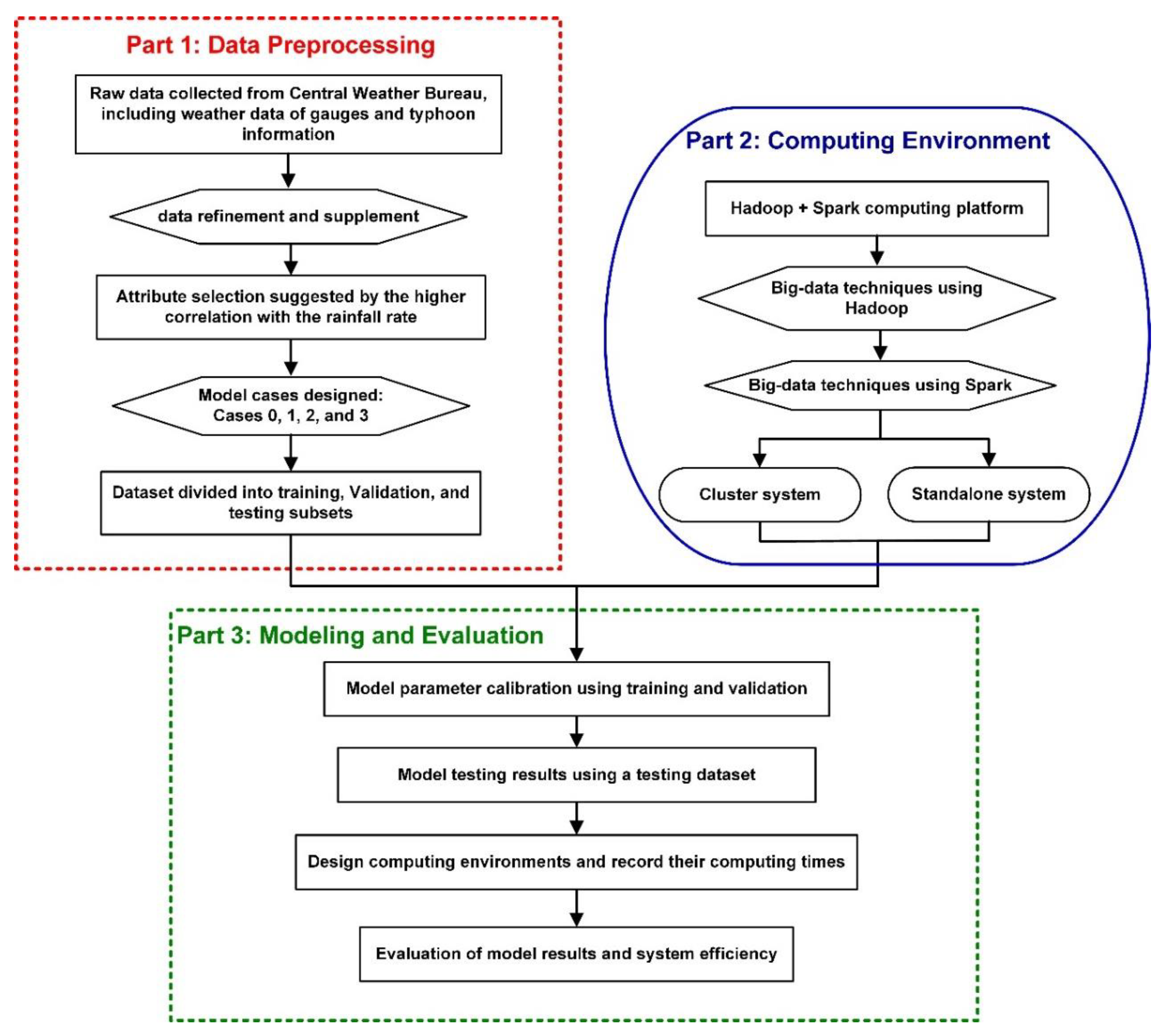
1. Introduction
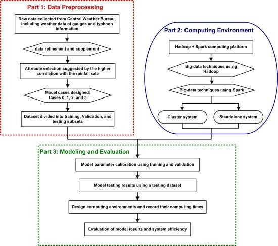
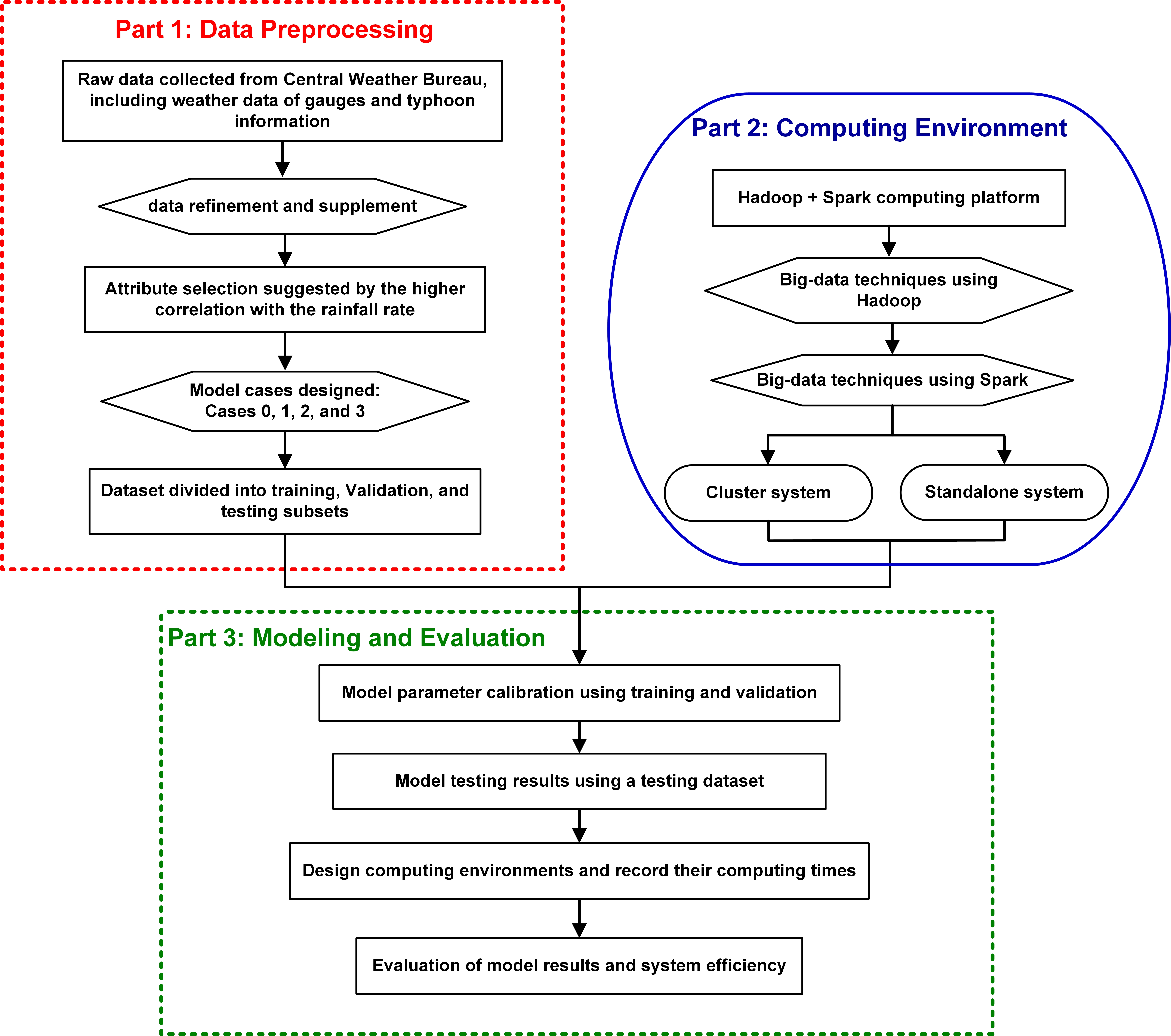
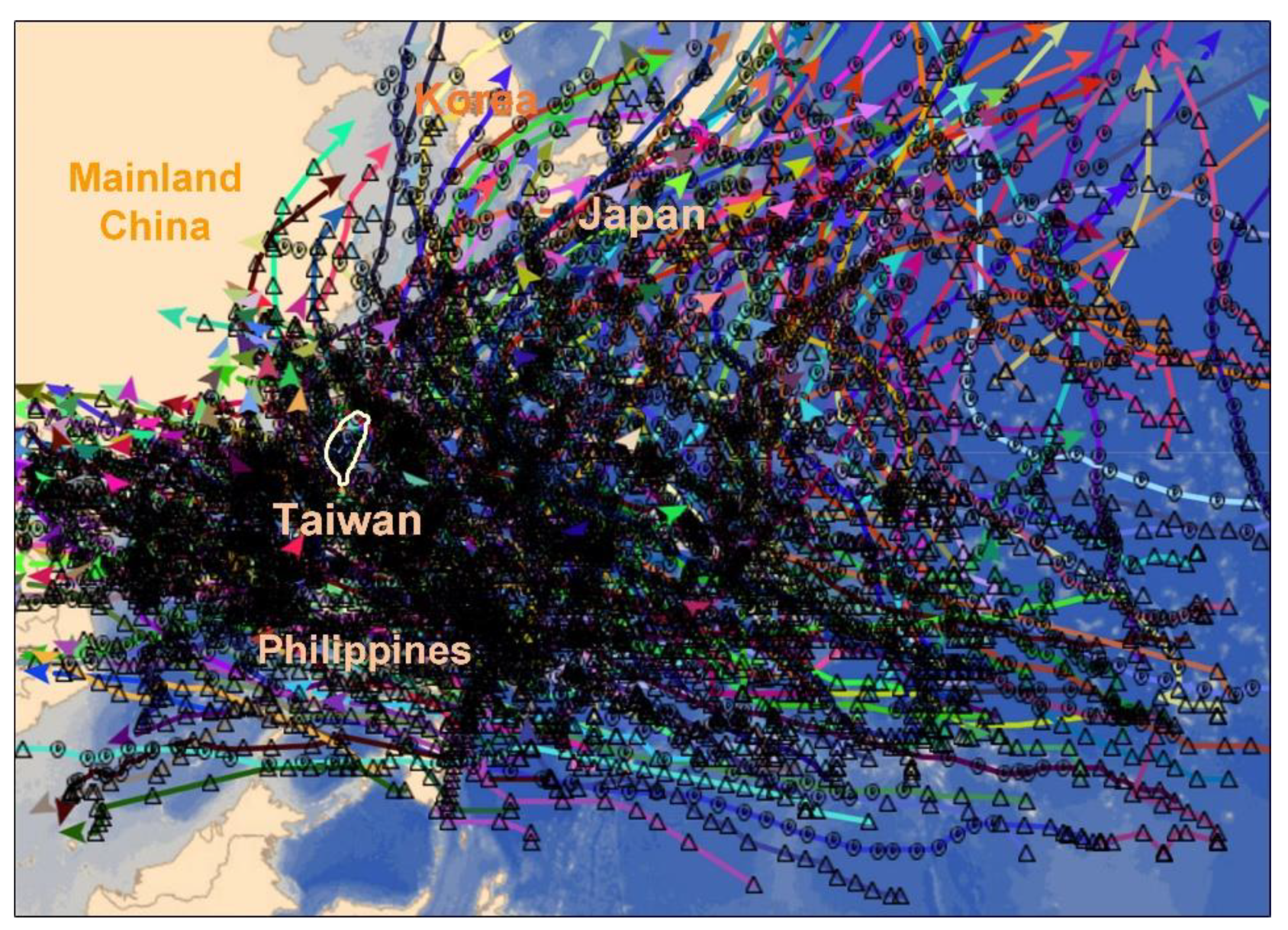
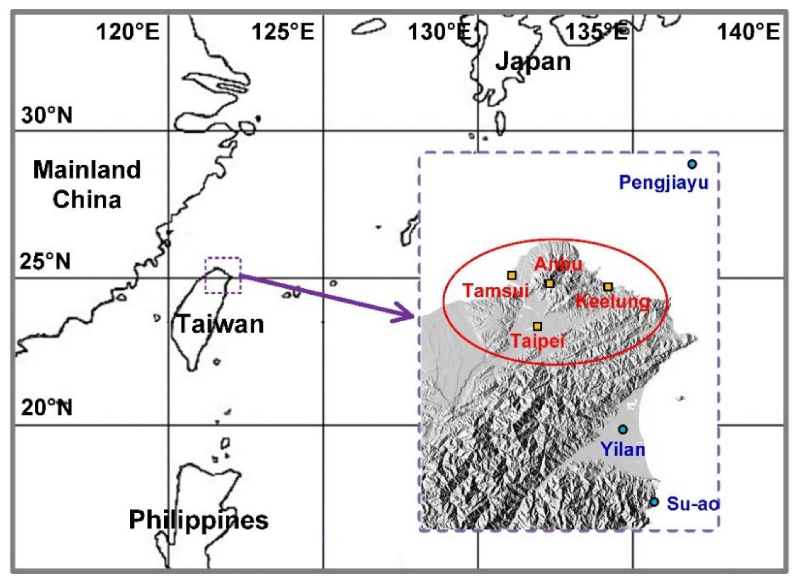
2. Data Sources and Preprocessing
3. Methodology
3.1. Data Division
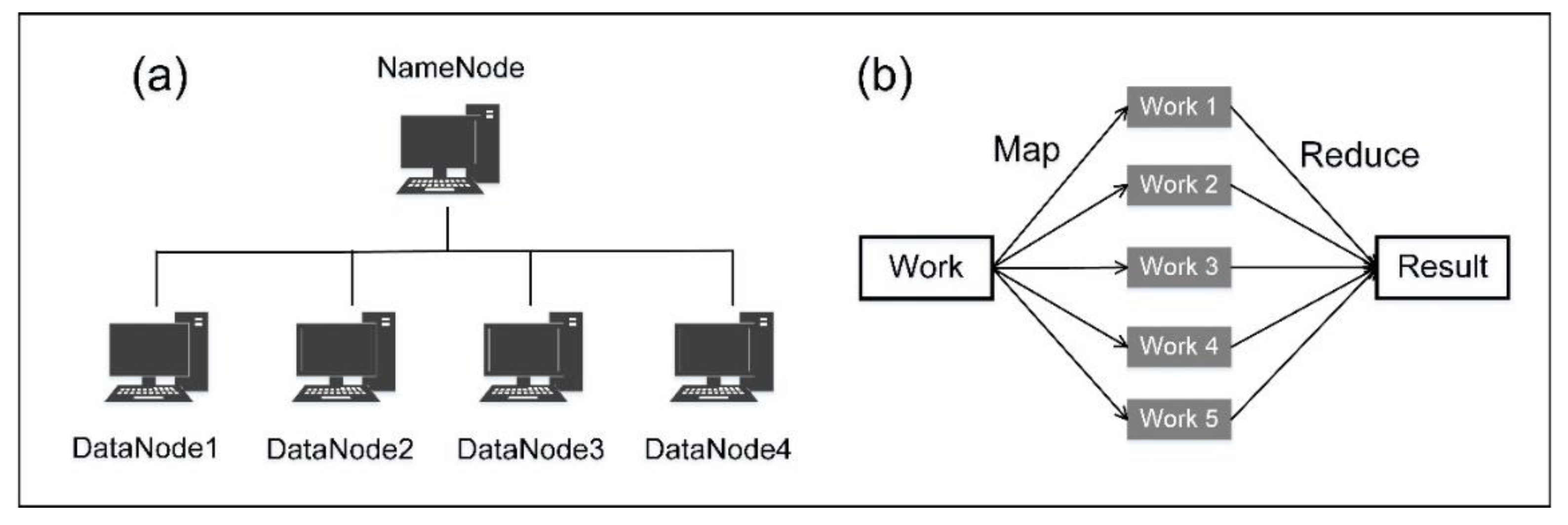
3.2. Computing Environment
4. Modeling and Evaluation
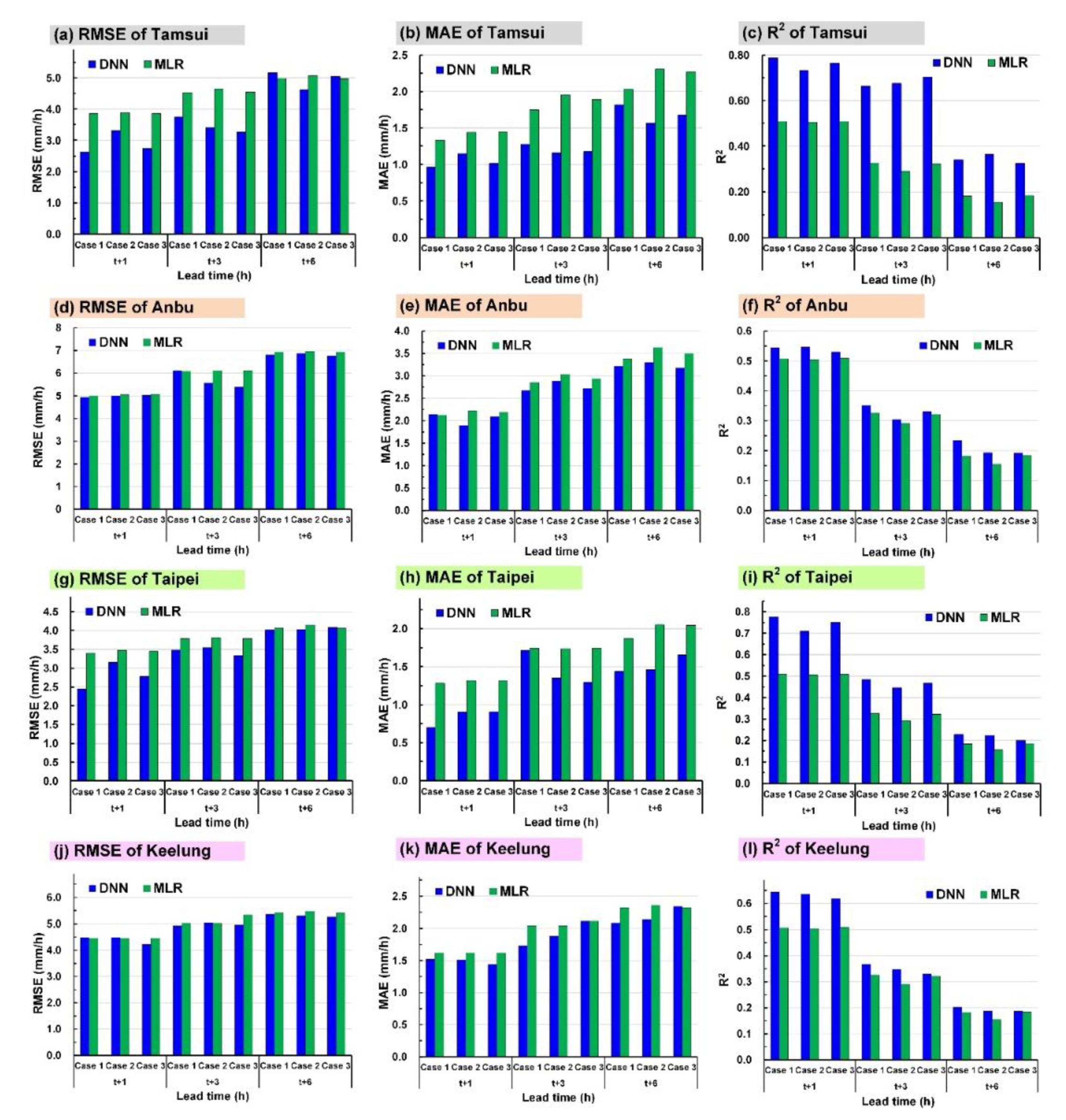
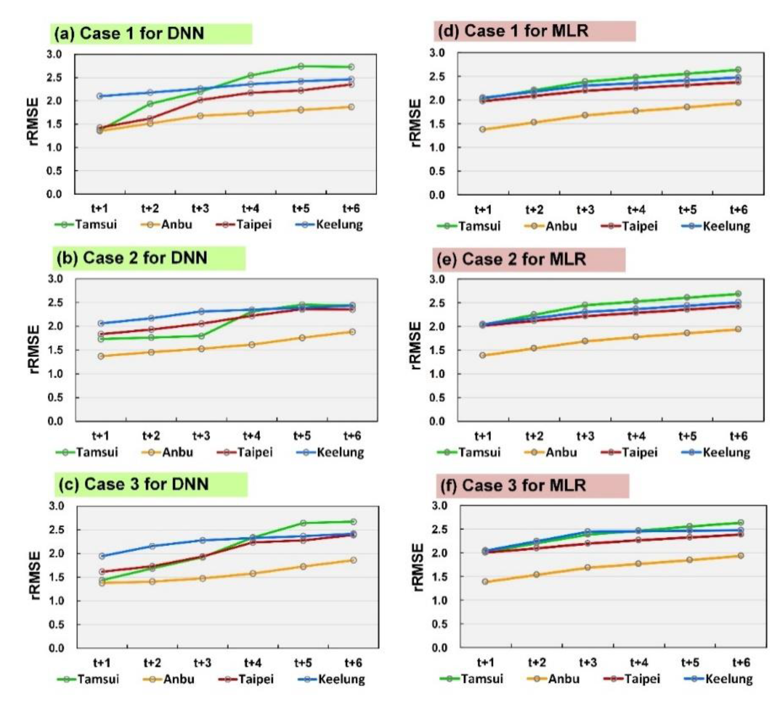
4.1. Results and Comparisons
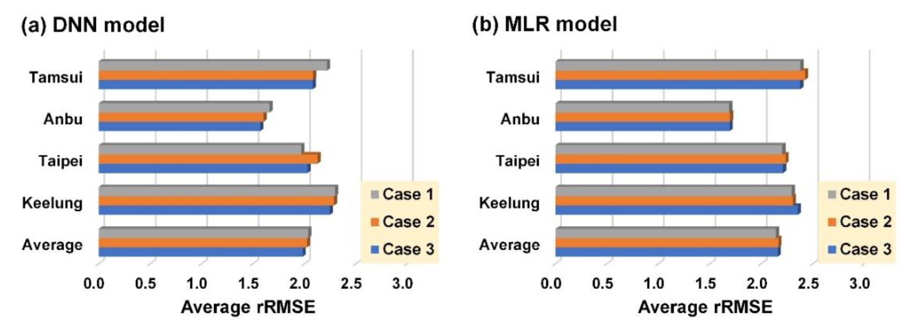
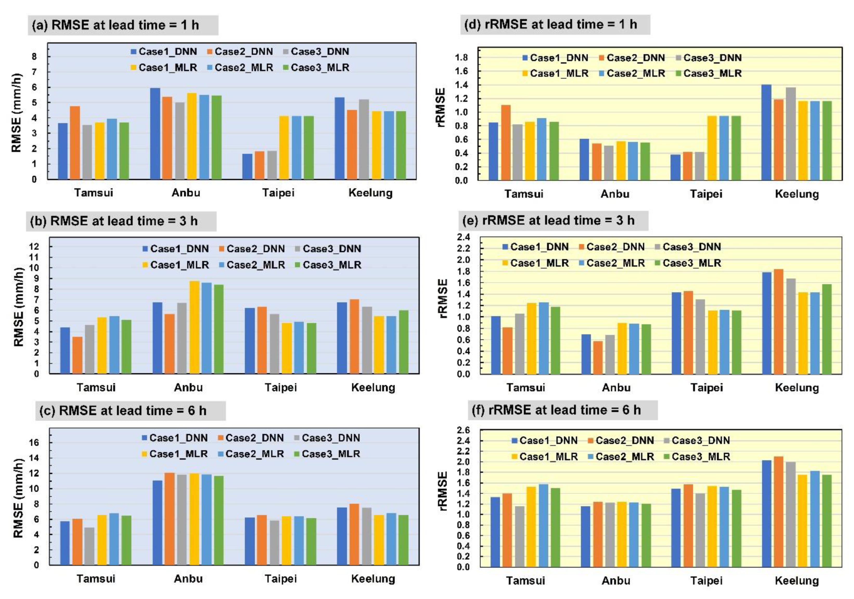
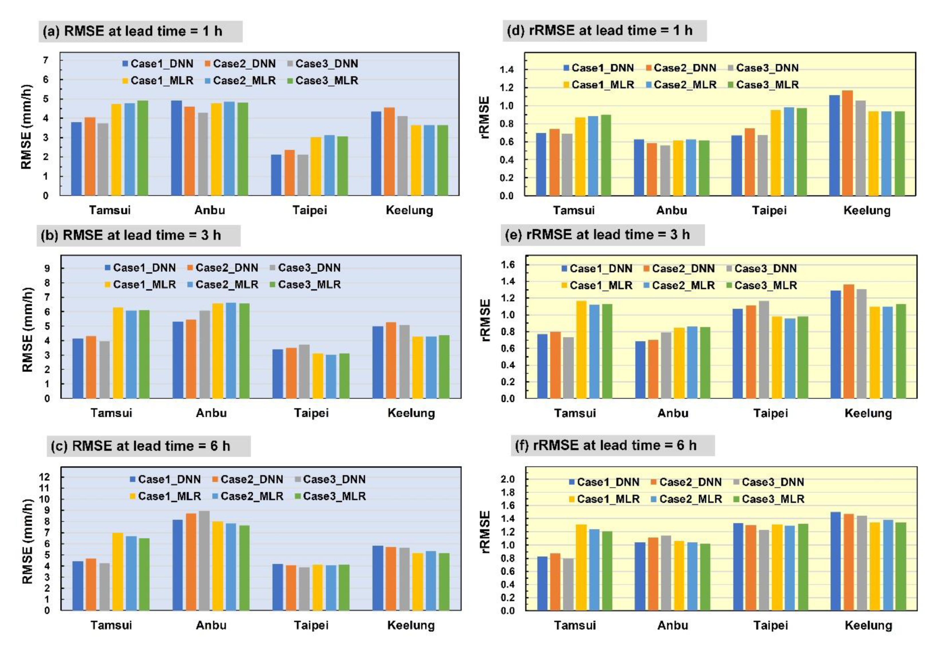
- In Case 1, the DNN model prediction result (Figure 6a) exhibited the most favorable performance in the Anbu station, followed by that in the Taipei, Tamsui, and Keelung stations. The MLR prediction results (Figure 6d) were most favorable in the Anbu station, followed by those in the Taipei, Keelung, and Tamsui stations (no significant difference was attained).
- In Case 2, the DNN prediction results (Figure 6b) were the most favorable in the Anbu station, followed by the Tamsui, Taipei, and Keelung stations. The MLR prediction results of the Anbu station were the most favorable (Figure 6e), followed by those in the Taipei, Keelung, and Tamsui stations (similar results).
- In Case 3, the DNN prediction results (Figure 6c) of the Anbu station were the most favorable, followed by those of the Taipei, Tamsui, and Keelung stations. The MLR prediction results of the Anbu station were the most favorable (Figure 6f), followed by those of the Taipei, Keelung, and Tamsui stations (with similar results).
4.2. Simulation of Typhoons
5. Efficiency of Computation Environments
6. Conclusions
Author Contributions
Funding
Acknowledgments
Conflicts of Interest
Appendix A. Typhoons and Data Attributes Over 1961–2017

| Year | Typhoon | Year | Typhoon | Year | Typhoon |
|---|---|---|---|---|---|
| 1961 | Betty, Elsie, June, Lorna, Pamela, Sally | 1980 | Ida, Norris, Percy, Betty | 1999 | Sam |
| 1962 | Kate, Opal, Wanda, Amy, Dinah | 1981 | Ike, June, Maury, Agnes, Clara, Irma | 2000 | Kai-tak, Bilis, Prapiroon, Bopha, Yagi, Xangsane, Bebinca |
| 1963 | Wendy, Gloria | 1982 | Andy, Cecil, Dot, Ken | 2001 | Cimaron, Chebi, Utor, Trami, |
| 1964 | Betty, Doris, Ida, Sally, Tilda | 1983 | Wayne, Ellen, Forrest | 2002 | Rammasun, Nakri, Sinlaku |
| 1965 | Dinah, Harriet | 1984 | Wynne, Alex, Freda, Holly, June | 2003 | Kujira, Nangka, Soudelor, Imbudo, Morakot, Vamco, Krovanh, Dujuan, Melor |
| 1966 | Judy, Alice, Cora, Elsie | 1985 | Hal, Jeff, Nelson, Val, Brenda | 2004 | Conson, Mindulle, |
| 1967 | Anita, Clara, Nora, Carla, Glida | 1986 | Nancy, Peggy, Wayne, Wayne, Wayne, Abby | 2005 | Haitang, Matsa, Sanvu, Talim, Khanun, Damrey, Longwang |
| 1968 | Wendy, Elaine | 1987 | Thelma, Vernon, Alex, Cary, Dinah, Gerald, Lynn | 2006 | Chanchu, Ewiniar, Bilis, Kaemi, Saomai, Bopha, Shanshan |
| 1969 | Viola, Betty, Elsie, Flossie | 1988 | Susan, Warren, Nelson | 2007 | Pabuk, Sepat, Wipha, Krosa, Mitag |
| 1970 | Olga, Wilda, Fran | 1989 | Sarah | 2008 | Kalmaegi, Fung-wong, Nuri, Sinlaku, Hagupit, Jangmi |
| 1971 | Lucy, Nadine, Agnes, Bess | 1990 | Marian, Ofelia, Percy, Robyn, Yancy, Abe, Dot | 2009 | Linfa, Molave, Morakot, Parma |
| 1972 | Susan, Winnie, Betty | 1991 | Amy, Brenda, Ellie, Mireille, Nat, Ruth, Seth | 2010 | Lionrock, Namtheun, Meranti, Fanapi, Megi |
| 1973 | Joan, Nora | 1992 | Bobbie, Mark, Omar, Polly, Ted | 2011 | Aere, Songda, Meari, Muifa, Nanmadol |
| 1974 | Jean, Lucy, Wendy, Bess | 1993 | Tasha, Yancy, Abe | 2012 | Talim, Doksuri, Saola, Haikui, Kai-tak, Tembin, Tembin, Jelawat |
| 1975 | Nina, Betty, Elsie | 1994 | Tim, Caitlin, Doug, Fred, Gladys, Seth | 2013 | Soulik, Cimaron, Trami, Kong-rey, Usagi, Fitow |
| 1976 | Ruby, Billie | 1995 | Deanna, Gary, Janis, Kent, Ryan | 2014 | Hagibis, Matmo, Fung-wong |
| 1977 | Ruth, Thelma, Vera, Amy | 1996 | Cam, Gloria, Herb, Sally, Zane | 2015 | Noul, Chan-hom, Linfa, Soudelor, Goni, Dujuan |
| 1978 | Olive, Rose, Della, Ora | 1997 | Winnie, Amber, Cass, Ivan | 2016 | Nepartak, Meranti, Malakas, Megi, Aere |
| 1979 | Gordon, Hope, Irving, Judy | 1998 | Nichole, Otto, Yanni, Zeb, Babs | 2017 | Nesat, Haitang, Hato, Guchol, Talim |
| Attribute | Range | Mean |
|---|---|---|
| Pressure at typhoon center (hPa) | 15–1000 | 957.6 |
| Latitude (°N) of typhoon center | 15–29.5 | 22.3 |
| Longitude (°E) of typhoon center | 113.2–133.7 | 122.4 |
| Radius of winds over 15.5 m/s (km) | 0–400 | 206.7 |
| Moving speed of typhoon (km/h) | 0–65 | 17.1 |
| Maximum wind speed of typhoon center (m/s) | 12–216 | 74.5 |
| Attribute | Tamsui Station | Anbu Station | ||
|---|---|---|---|---|
| Range | Mean | Range | Mean | |
| Air pressure on the ground (hPa) | 957–1022 | 1000.5 | 871–929 | 912.2 |
| Temperature on the ground (°C) | 15.1–38.2 | 27.2 | 9.5–30.2 | 21.4 |
| Dew point on the ground (°C) | 10.8–30 | 23.1 | 8.5–25.4 | 20.2 |
| Relative humidity (%) | 2.4–100 | 79.5 | 42–100 | 93.0 |
| Vapor pressure on the ground (hPa) | 11.3–42.4 | 28.5 | 11.1–34.1 | 23.8 |
| Surface wind velocity (m/s) | 0–29.3 | 3.7 | 0–41.8 | 6.5 |
| Surface wind direction (°) | 0–360 | 140.4 | 0–360 | 228.3 |
| Precipitation (mm) | 0–86.8 | 1.3 | 0–119.5 | 2.9 |
| Attribute | Taipei Station | Keelung Station | ||
|---|---|---|---|---|
| Range | Mean | Range | Mean | |
| Air pressure on the ground (hPa) | 954–1023 | 1001.6 | 954–1021 | 1000.5 |
| Temperature on the ground (°C) | 16.1–37.3 | 27.5 | 15.6–36.7 | 27.3 |
| Dew point on the ground (°C) | 11.2–28.5 | 23.3 | 9.4–28.6 | 23.4 |
| Relative humidity (%) | 37–100 | 78.9 | 46–100 | 80.1 |
| Vapor pressure on the ground (hPa) | 13.3–38.9 | 28.8 | 11.8–37.1 | 29.0 |
| Surface wind velocity (m/s) | 0–28.9 | 3.9 | 0–28.5 | 5.0 |
| Surface wind direction (°) | 0–360 | 134.9 | 0–360 | 131.7 |
| Precipitation (mm) | 0–76 | 1.3 | 0–95.3 | 1.4 |
References
- Wei, C.C. Study on wind simulations using deep learning techniques during typhoons: A case study of Northern Taiwan. Atmosphere 2019, 10, 684. [Google Scholar] [CrossRef] [Green Version]
- Kang, S.C.; Shiu, R.S.; Wu, T.H. Development of typhoon search program with human manipulation consideration. In Proceedings of the Conference for Disaster Management in Taiwan, Disaster Management Society of Taiwan, Taipei, Taiwan, 16 November 2012. [Google Scholar]
- Wei, C.C.; Cheng, J.Y. Nearshore two-step typhoon wind-wave prediction using deep recurrent neural networks. J. Hydroinform. 2020, 22, 356–367. [Google Scholar] [CrossRef]
- Burgin, M.; Klinger, A. Experience, generations, and limits in machine learning. Theor. Comput. Sci. 2004, 317, 71–91. [Google Scholar] [CrossRef]
- Wei, C.C. Radial basis function networks combined with principal component analysis to typhoon precipitation forecast in a reservoir watershed. J. Hydrometeorol. 2012, 13, 722–734. [Google Scholar] [CrossRef]
- Schmidhuber, J. Deep learning in neural networks: An overview. Neural Netw. 2015, 61, 85–117. [Google Scholar] [CrossRef] [PubMed] [Green Version]
- Yeh, T.C. Typhoon rainfall over Taiwan area: The empirical orthogonal function modes and their applications on the rainfall forecasting. Terr. Atmos. Ocean. Sci. 2002, 13, 449–468. [Google Scholar] [CrossRef] [Green Version]
- Lee, C.S.; Huang, L.R.; Shen, H.S.; Wang, S.T. A climatology model for forecasting typhoon rainfall in Taiwan. Nat. Hazards 2006, 37, 87–105. [Google Scholar] [CrossRef]
- Hsu, N.S.; Wei, C.C. A multipurpose reservoir real-time operation model for flood control during typhoon invasion. J. Hydrol. 2007, 336, 282–293. [Google Scholar] [CrossRef]
- Hall, T.; Brooks, H.E.; Doswell, C.A. Precipitation forecasting using a neural network. Weather Forecast. 1999, 14, 338–345. [Google Scholar] [CrossRef] [Green Version]
- Fox, N.I.; Wikle, C.K. A Bayesian quantitative precipitation nowcast scheme. Weather Forecast. 2005, 20, 264–275. [Google Scholar] [CrossRef] [Green Version]
- Nasseri, M.; Asghari, K.; Abedini, M.J. Optimized scenario for rainfall forecasting using genetic algorithm coupled with artificial neural network. Expert Syst. Appl. 2008, 35, 1415–1421. [Google Scholar] [CrossRef]
- Biondi, D.; De Luca, D.L. A Bayesian approach for real-time flood forecasting. Phys. Chem. Earth 2012, 42–44, 91–97. [Google Scholar] [CrossRef]
- Wei, C.C. Wavelet support vector machines for forecasting precipitations in tropical cyclones: Comparisons with GSVM, regressions, and numerical MM5 model. Weather Forecast. 2012, 27, 438–450. [Google Scholar] [CrossRef]
- Kühnlein, M.; Appelhans, T.; Thies, B.; Nauß, T. Precipitation estimates from MSG SEVIRI daytime, nighttime, and twilight data with random forests. J. Appl. Meteorol. Climatol. 2014, 53, 2457–2480. [Google Scholar] [CrossRef] [Green Version]
- Wei, C.C. Simulation of operational typhoon rainfall nowcasting using radar reflectivity combined with meteorological data. J. Geophys. Res. Atmos. 2014, 119, 6578–6595. [Google Scholar] [CrossRef]
- Wei, C.C.; You, G.J.Y.; Chen, L.; Chou, C.C.; Roan, J. Diagnosing rain occurrences using passive microwave imagery: A comparative study on probabilistic graphical models and “black box” models. J. Atmos. Ocean. Technol. 2015, 32, 1729–1744. [Google Scholar] [CrossRef]
- Diez-Sierra, J.; del Jesus, M. Subdaily rainfall estimation through daily rainfall downscaling using random forests in Spain. Water 2019, 11, 125. [Google Scholar] [CrossRef] [Green Version]
- Ko, C.M.; Jeong, Y.Y.; Lee, Y.M.; Kim, B.S. The development of a quantitative precipitation forecast correction technique based on machine learning for hydrological applications. Atmosphere 2020, 11, 111. [Google Scholar] [CrossRef] [Green Version]
- Xiang, B.; Zeng, C.; Dong, X.; Wang, J. The application of a decision tree and stochastic forest model in summer precipitation prediction in Chongqing. Atmosphere 2020, 11, 508. [Google Scholar] [CrossRef]
- Asklany, S.A.; Elhelow, K.; Youssef, I.K.; El-wahab, M.A. Rainfall events prediction using rule-based fuzzy inference system. Atmos. Res. 2011, 101, 228–236. [Google Scholar] [CrossRef]
- Maier, H.R.; Dandy, G.C. Neural networks for the prediction and forecasting of water resources variables: A review of modeling issues and applications. Environ. Model. Softw. 2000, 15, 101–124. [Google Scholar] [CrossRef]
- Antolik, M.S. An overview of the National Weather Service’s centralized statistical quantitative precipitation forecasts. J. Hydrol. 2000, 239, 306–337. [Google Scholar] [CrossRef]
- Maier, H.R.; Jain, A.; Dandy, G.C.; Sudheer, K. Methods used for the development of neural networks for the prediction of water resource variables in river systems: Current status and future directions. Environ. Model. Softw. 2010, 25, 891–909. [Google Scholar] [CrossRef]
- Madsen, H.; Lawrence, D.; Lang, M.; Martinkova, M.; Kjeldsen, T.R. Review of trend analysis and climate change projections of extreme precipitation and floods in Europe. J. Hydrol. 2014, 519, 3634–3650. [Google Scholar] [CrossRef] [Green Version]
- Maçaira, P.; Thomé, A.M.; Oliveira, F.L.; Ferrer, A.L. Time series analysis with explanatory variables: A systematic literature review. Environ. Model. Softw. 2018, 107, 199–209. [Google Scholar] [CrossRef]
- Paulo Vitor de Campos Souza, P.V. Fuzzy neural networks and neuro-fuzzy networks: A review the main techniques and applications used in the literature. Appl. Soft Comput. 2020, 92, 106275. [Google Scholar] [CrossRef]
- Tao, Y.; Gao, X.; Ihler, A.; Sorooshian, S.; Hsu, K. Precipitation identification with bispectral satellite information using deep learning approaches. J. Hydrometeorol. 2017, 18, 1271–1283. [Google Scholar] [CrossRef]
- Wang, H.Z.; Wang, G.B.; Li, G.Q.; Peng, J.C.; Liu, Y.T. Deep belief network based deterministic and probabilistic wind speed forecasting approach. Appl. Energy 2016, 182, 80–93. [Google Scholar] [CrossRef]
- Wang, J.H.; Lin, G.F.; Chang, M.J.; Huang, I.H.; Chen, Y.R. Real-time water-level forecasting using dilated causal convolutional neural networks. Water Resour. Manag. 2019, 33, 3759–3780. [Google Scholar] [CrossRef]
- Wei, C.C.; Hsieh, P.Y. Estimation of hourly rainfall during typhoons using radar mosaic-based convolutional neural networks. Remote Sens. 2020, 12, 896. [Google Scholar] [CrossRef] [Green Version]
- Emani, C.K.; Cullot, N.; Nicolle, C. Understandable big data: A survey. Comput. Sci. Rev. 2015, 17, 70–81. [Google Scholar] [CrossRef]
- Qureshi, B.; Koubaa, A. On energy efficiency and performance evaluation of single board computer based clusters: A Hadoop case study. Electronics 2019, 8, 182. [Google Scholar] [CrossRef] [Green Version]
- Zaharia, M.; Xin, R.S.; Wendell, P.; Das, T.; Armbrust, M.; Dave, A.; Meng, X.; Rosen, J.; Venkataraman, S.; Franklin, M.J. Apache Spark: A unified engine for big data processing. Commun. Acm 2016, 59, 56–65. [Google Scholar] [CrossRef]
- International Data Corporation (IDC). Big Data Big Opportunities. 2018. Available online: http://www.emc.com/microsites/cio/articles/big-data-bigopportunities/LCIA-BigDataOpportunities-Value.pdf (accessed on 25 July 2018).
- Dailey, W. The Big Data Technology Wave. 2019. Available online: https://www.skillsoft.com/courses/5372828-thebig-data-technology-wave/ (accessed on 18 March 2019).
- Borthakur, D. The Hadoop Distributed File System: Architecture and Design. 2007. Hadoop Projection Website. Available online: http://svn.apache.org/repos/asf/hadoop/common/tags/release-0.16.3/docs/hdfs_design.pdf (accessed on 1 July 2020).
- Dean, J.; Ghemawat, S. MapReduce: Simplified data processing on large clusters. Commun. Acm 2008, 51, 107–113. [Google Scholar] [CrossRef]
- Bechini, A.; Marcelloni, F.; Segatori, A. A MapReduce solution for associative classification of big data. Inf. Sci. 2016, 332, 33–55. [Google Scholar] [CrossRef] [Green Version]
- Armbrust, M.; Xin, R.S.; Lian, C.; Huai, Y.; Liu, D.; Bradley, J.K.; Meng, X.; Kaftan, T.; Franklin, M.J.; Ghodsi, A. Spark SQL: Relational Data Processing in Spark. In Proceedings of the ACM SIGMOD/PODS Conference, Melbourne, Australia, 31 May– 4 June 2015; ACM Press: New York, NY, USA, 2015. [Google Scholar]
- Xin, R.S.; Rosen, J.; Zaharia, M.; Franklin, M.J.; Shenker, S.; Stoica, I. Shark: SQL and Rich Analytics at Scale. In Proceedings of the ACM SIGMOD/PODS Conference, New York, NY, USA, 22–27 June 2013; ACM Press: New York, NY, USA, 2013. [Google Scholar]
- Hu, Y.; Cai, X.; DuPont, B. Design of a web-based application of the coupled multi-agent system model and environmental model for watershed management analysis using Hadoop. Environ. Model. Softw. 2015, 70, 149–162. [Google Scholar] [CrossRef]
- Hu, Y.; Garcia-Cabrejo, O.; Cai, X.; Valocchi, A.J.; DuPont, B. Global sensitivity analysis for large-scale socio-hydrological models using Hadoop. Environ. Model. Softw. 2015, 73, 231–243. [Google Scholar] [CrossRef]
- Taylor, R. Interpretation of the correlation coefficient: A basic review. J. Diagn. Med Sonogr. 1990, 1, 35–39. [Google Scholar] [CrossRef]
- Central Weather Bureau (CWB). 2019. Available online: http://www.cwb.gov.tw/V8/C/K/announce.html (accessed on 1 December 2019).
- Villegas-Ch, W.; Palacios-Pacheco, X.; Luján-Mora, S. Application of a smart city model to a traditional university campus with a big data architecture: A sustainable smart campus. Sustainability 2019, 11, 2857. [Google Scholar] [CrossRef] [Green Version]
- Ajah, I.A.; Nweke, H.F. Big data and business analytics: Trends, platforms, success factors and applications. Big Data Cogn. Comput. 2019, 3, 32. [Google Scholar] [CrossRef] [Green Version]
- Hashem, I.A.T.; Yaqoob, I.; Anuar, N.B.; Mokhtar, S.; Gani, A.; Khan, S.U. The rise of “big data” on cloud computing: Review and open research issues. Inf. Syst. 2015, 47, 98–115. [Google Scholar] [CrossRef]
- Lin, C.; Wei, C.C.; Tsai, C.C. Prediction of influential operational compost parameters for monitoring composting process. Environ. Eng. Sci. 2016, 33, 494–506. [Google Scholar] [CrossRef]
- Genell, A.; Nemes, S.; Steineck, G.; Dickman, P.W. Model selection in medical research: A simulation study comparing Bayesian model averaging and stepwise regression. BMC Med Res. Methodol. 2010, 10, 108. [Google Scholar] [CrossRef] [PubMed] [Green Version]
- Wei, C.C. Comparing lazy and eager learning models for water level forecasting in river-reservoir basins of inundation regions. Environ. Model. Softw. 2015, 63, 137–155. [Google Scholar] [CrossRef]
- Wu, W.; May, R.J.; Maier, H.R.; Dandy, G.C. A benchmarking approach for comparing data splitting methods for modeling water resources parameters using artificial neural networks. Water Resour. Res. 2013, 49, 7598–7614. [Google Scholar] [CrossRef]
- Bennett, N.D.; Croke, B.; Guariso, G.; Guillaume, J.H.A.; Hamilton, S.H.; Jakeman, A.; Marsili-Libelli, S.; Newham, L.T.; Norton, J.P.; Perrin, C.; et al. Characterising performance of environmental models. Environ. Model. Softw. 2013, 40, 1–20. [Google Scholar] [CrossRef]
- Wei, C.C. Comparing single- and two-segment statistical models with a conceptual rainfall-runoff model for river streamflow prediction during typhoons. Environ. Model. Softw. 2016, 85, 112–128. [Google Scholar] [CrossRef] [Green Version]
- Efroymson, M.A. Multiple Regression Analysis; Ralston, A., Wilf, H.S., Eds.; Mathematical Methods for Digital Computers, John Wiley: New York, NY, USA, 1960; pp. 191–203. [Google Scholar]


| Station | Latitude (°N) | Longitude (°E) | Altitude (m) |
|---|---|---|---|
| Tamsui | 25.1649 | 121.4489 | 19 |
| Anbu | 25.1826 | 121.5297 | 826 |
| Taipei | 25.0377 | 121.5149 | 7 |
| Keelung | 25.1333 | 121.7405 | 27 |
| Pengjiayu | 25.6280 | 122.0797 | 102 |
| Su-ao | 24.5967 | 121.8574 | 25 |
| Yilan | 24.7640 | 121.7565 | 8 |
| Target Station | Selected Attributes |
|---|---|
| Tamsui | W2, Y4, and Y8 of Tamsui; Y8 of Anbu; Y4 and Y8 of Taipei; Y4, Y6, and Y8 of Keelung; Y4, Y6, and Y8 of Pengjiayu; Y1 of Su-ao; Y1 and Y8 of Yilan |
| Anbu | Y2, Y4, Y6, and Y8 of Tamsui; W2 and Y8 of Anbu; Y2, Y4, and Y8 of Taipei; Y2, Y4, Y6, and Y8 of Keelung; Y6 and Y8 of Pengjiayu; Y1 and Y8 of Su-ao; Y1, Y6, and Y8 of Yilan |
| Taipei | Y4 and Y8 of Tamsui; Y1 and Y8 of Anbu; W2, Y4, and Y8 of Taipei; Y4, Y6, and Y8 of Keelung; Y1 and Y6 of Pengjiayu; Y1 of Su-ao; Y1 and Y8 of Yilan |
| Keelung | Y8 of Tamsui; Y8 of Anbu; Y4 and Y8 of Taipei; W2, Y4, Y6, and Y8 of Keelung; Y6 and Y8 of Pengjiayu; Y8 of Su-ao; Y8 of Yilan |
| Equipment | Cluster System | Standalone PC |
|---|---|---|
| Brand and model | ASUS-TS300E9 | GIGABYTE-P55 |
| CPU | E3-1240v6 (3.5GHz) | I7-6700HQ (3.5GHz) |
| Chipset | Intel C236 Chipset | Intel C236 Chipset |
| Memory | DDR4-240016G | DDR4-240016G |
| Number of computers | 4 | 1 |
| Name | IP Address | HDFS | YARN |
|---|---|---|---|
| master | 192.168.0.100 | NameNode | ResourceManager |
| data1 | 192.168.0.101 | DataNode | NodeManager |
| data2 | 192.168.0.102 | DataNode | NodeManager |
| data3 | 192.168.0.103 | DataNode | NodeManager |
| Station | Case | Parameter | Lead Time (h) | |||||
|---|---|---|---|---|---|---|---|---|
| 1 | 2 | 3 | 4 | 5 | 6 | |||
| Tamsui | 1 | Layers 1–3 | (6,4,6) | (2,1,5) | (1,2,6) | (1,2,1) | (1,1,1) | (1,1,1) |
| Learning rate | 0.3 | 0.1 | 0.2 | 0.1 | 0.4 | 0.2 | ||
| 2 | Layers 1–3 | (3,2,4) | (2,3,2) | (2,1,3) | (3,2,4) | (3,3,1) | (3,3,5) | |
| Learning rate | 0.6 | 0.4 | 0.3 | 0.1 | 0.1 | 0.1 | ||
| 3 | Layers 1–3 | (1,6,4) | (2,5,4) | (3,7,3) | (1,3,1) | (1,3,6) | (1,3,4) | |
| Learning rate | 0.2 | 0.2 | 0.1 | 0.1 | 0.1 | 0.1 | ||
| Anbu | 1 | Layers 1–3 | (7,4,8) | (6,3,4) | (6,4,4) | (6,3,2) | (4,5,6) | (5,5,7) |
| Learning rate | 0.4 | 0.4 | 0.3 | 0.4 | 0.3 | 0.3 | ||
| 2 | Layers 1–3 | (3,6,4) | (3,5,4) | (3,4,5) | (3,3,4) | (6,4,5) | (5,3,6) | |
| Learning rate | 0.5 | 0.3 | 0.2 | 0.2 | 0.5 | 0.4 | ||
| 3 | Layers 1–3 | (4,7,7) | (3,5,7) | (3,6,7) | (2,5,1) | (3,5,3) | (5,4,6) | |
| Learning rate | 0.4 | 0.3 | 0.4 | 0.4 | 0.3 | 0.2 | ||
| Taipei | 1 | Layers 1–3 | (4,3,5) | (1,3,3) | (1,2,2) | (1,2,1) | (1,3,5) | (1,1,1) |
| Learning rate | 0.3 | 0.3 | 0.3 | 0.2 | 0.1 | 0.1 | ||
| 2 | Layers 1–3 | (2,6,2) | (2,5,7) | (1,5,4) | (2,3,5) | (2,5,2) | (4,4,1) | |
| Learning rate | 0.7 | 0.1 | 0.1 | 0.2 | 0.1 | 0.1 | ||
| 3 | Layers 1–3 | (1,8,6) | (1,5,3) | (2,6,7) | (2,5,4) | (5,1,1) | (2,3,3) | |
| Learning rate | 0.6 | 0.1 | 0.1 | 0.1 | 0.3 | 0.1 | ||
| Keelung | 1 | Layers 1–3 | (3,1,1) | (3,2,2) | (5,1,1) | (4,2,2) | (4,4,2) | (5,4,4) |
| Learning rate | 0.1 | 0.2 | 0.1 | 0.3 | 0.1 | 0.1 | ||
| 2 | Layers 1–3 | (6,4,2) | (4,3,5) | (3,3,5) | (3,2,3) | (2,3,7) | (1,2,5) | |
| Learning rate | 0.1 | 0.3 | 0.1 | 0.1 | 0.1 | 0.1 | ||
| 3 | Layers 1–3 | (5,5,6) | (5,3,5) | (3,1,2) | (4,2,1) | (2,3,3) | (1,3,2) | |
| Learning rate | 0.1 | 0.1 | 0.1 | 0.1 | 0.1 | 0.1 | ||
| Station | Model | Standalone (I7) | Single Server (E3) | Cluster System (Hadoop) | |||
|---|---|---|---|---|---|---|---|
| USER | CPU | USER | CPU | USER | CPU | ||
| Tamsui | MLR | 0.58 | 0.13 | 0.56 | 0.05 | 0.58 | 0.05 |
| DNN | 2134.0 | 175.6 | 697.5 | 59.1 | 76.4 | 8.6 | |
| Anbu | MLR | 0.95 | 0.21 | 0.70 | 0.18 | 0.58 | 0.06 |
| DNN | 2299.6 | 200.1 | 751.6 | 67.3 | 82.3 | 9.8 | |
| Taipei | MLR | 0.58 | 0.08 | 0.57 | 0.07 | 0.56 | 0.06 |
| DNN | 2252.7 | 216.4 | 736.3 | 72.8 | 80.6 | 10.6 | |
| Keelung | MLR | 0.47 | 0.14 | 0.50 | 0.05 | 0.47 | 0.05 |
| DNN | 2043.7 | 157.7 | 667.9 | 53.0 | 73.2 | 7.7 | |
| Average | MLR | 0.65 | 0.14 | 0.58 | 0.09 | 0.55 | 0.05 |
| DNN | 2182.5 | 187.5 | 713.3 | 63.0 | 78.1 | 9.2 | |
© 2020 by the authors. Licensee MDPI, Basel, Switzerland. This article is an open access article distributed under the terms and conditions of the Creative Commons Attribution (CC BY) license (http://creativecommons.org/licenses/by/4.0/).
Share and Cite
Wei, C.-C.; Chou, T.-H. Typhoon Quantitative Rainfall Prediction from Big Data Analytics by Using the Apache Hadoop Spark Parallel Computing Framework. Atmosphere 2020, 11, 870. https://doi.org/10.3390/atmos11080870
Wei C-C, Chou T-H. Typhoon Quantitative Rainfall Prediction from Big Data Analytics by Using the Apache Hadoop Spark Parallel Computing Framework. Atmosphere. 2020; 11(8):870. https://doi.org/10.3390/atmos11080870
Chicago/Turabian StyleWei, Chih-Chiang, and Tzu-Hao Chou. 2020. "Typhoon Quantitative Rainfall Prediction from Big Data Analytics by Using the Apache Hadoop Spark Parallel Computing Framework" Atmosphere 11, no. 8: 870. https://doi.org/10.3390/atmos11080870