Future Changes in the Free Tropospheric Freezing Level and Rain–Snow Limit: The Case of Central Chile


Abstract
:1. Introduction
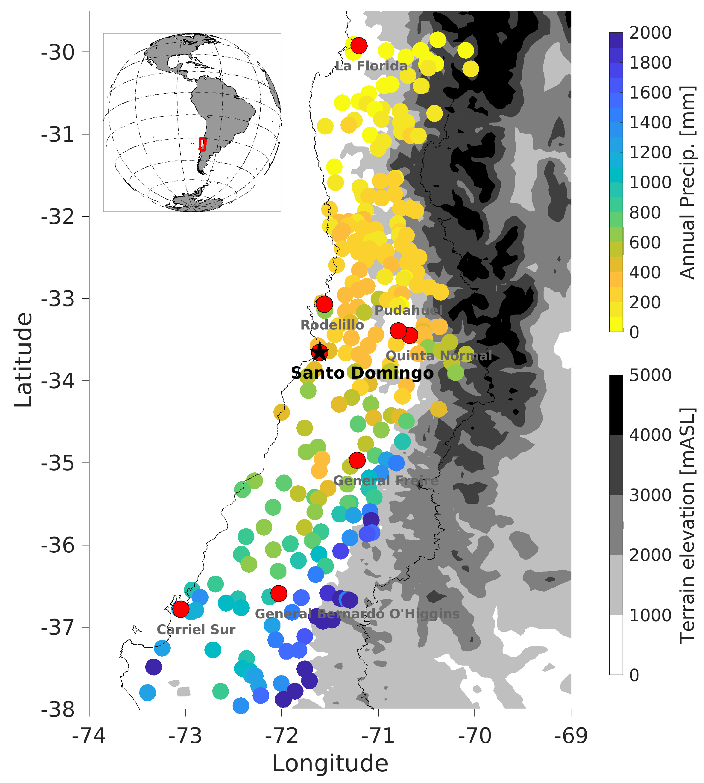
2. Study Region
3. Data and Models
3.1. Observations
3.2. Reanalysis
3.3. Models
4. Results and Discussion
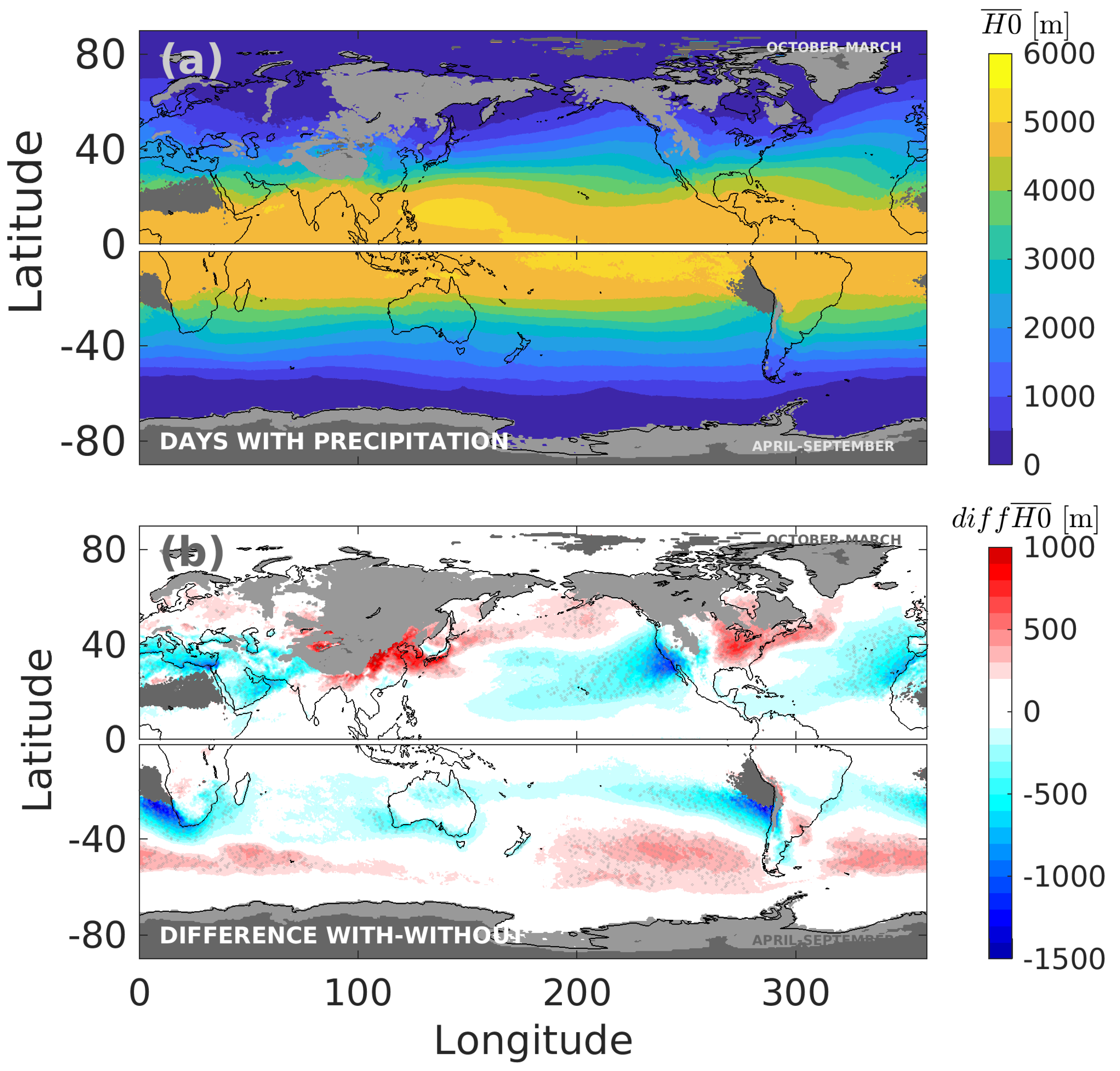
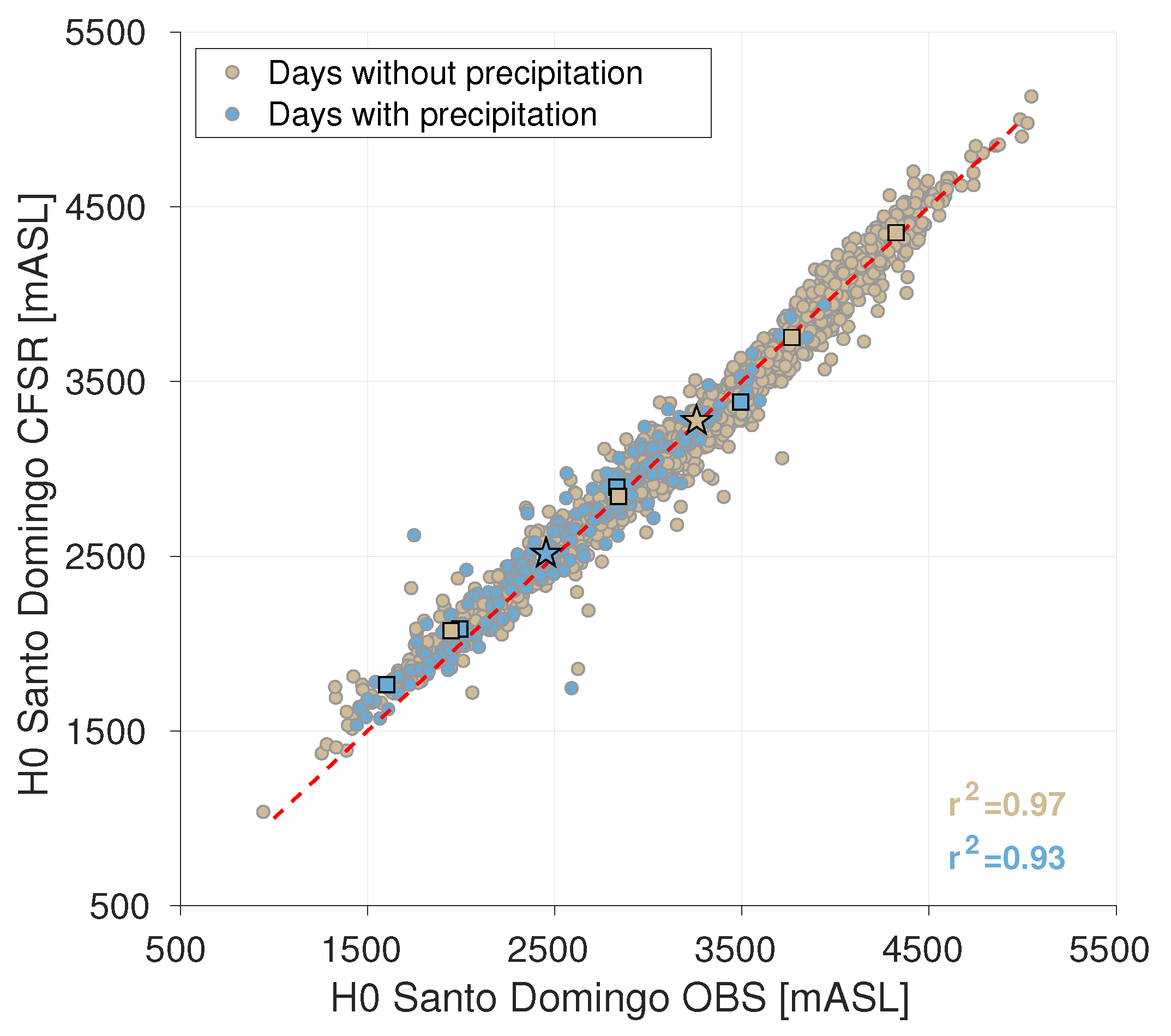
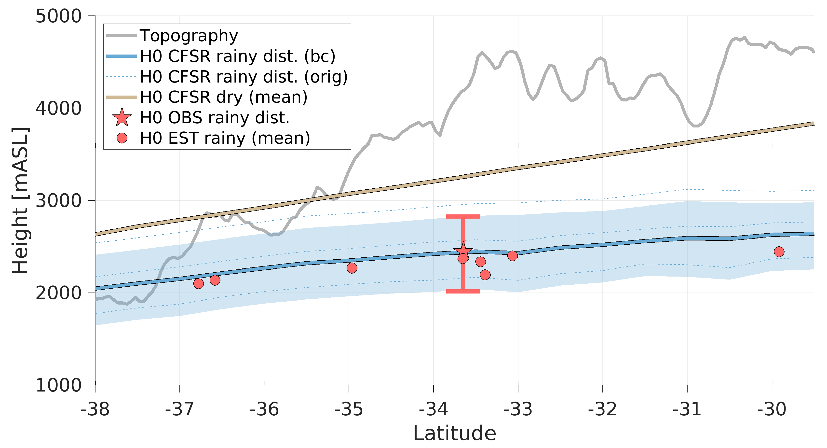
4.1. The Freezing Level in Present Climate
4.2. Future Changes
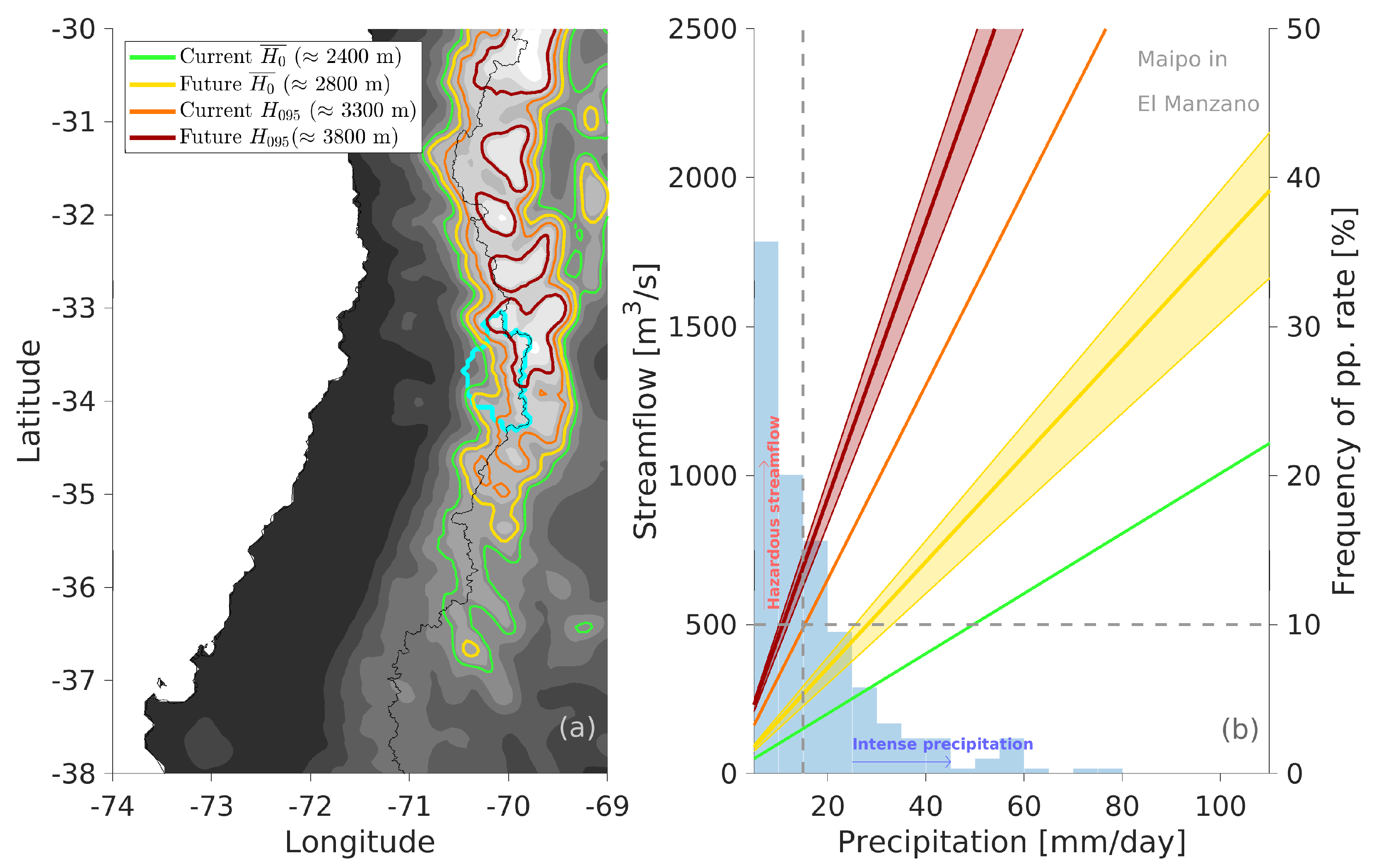
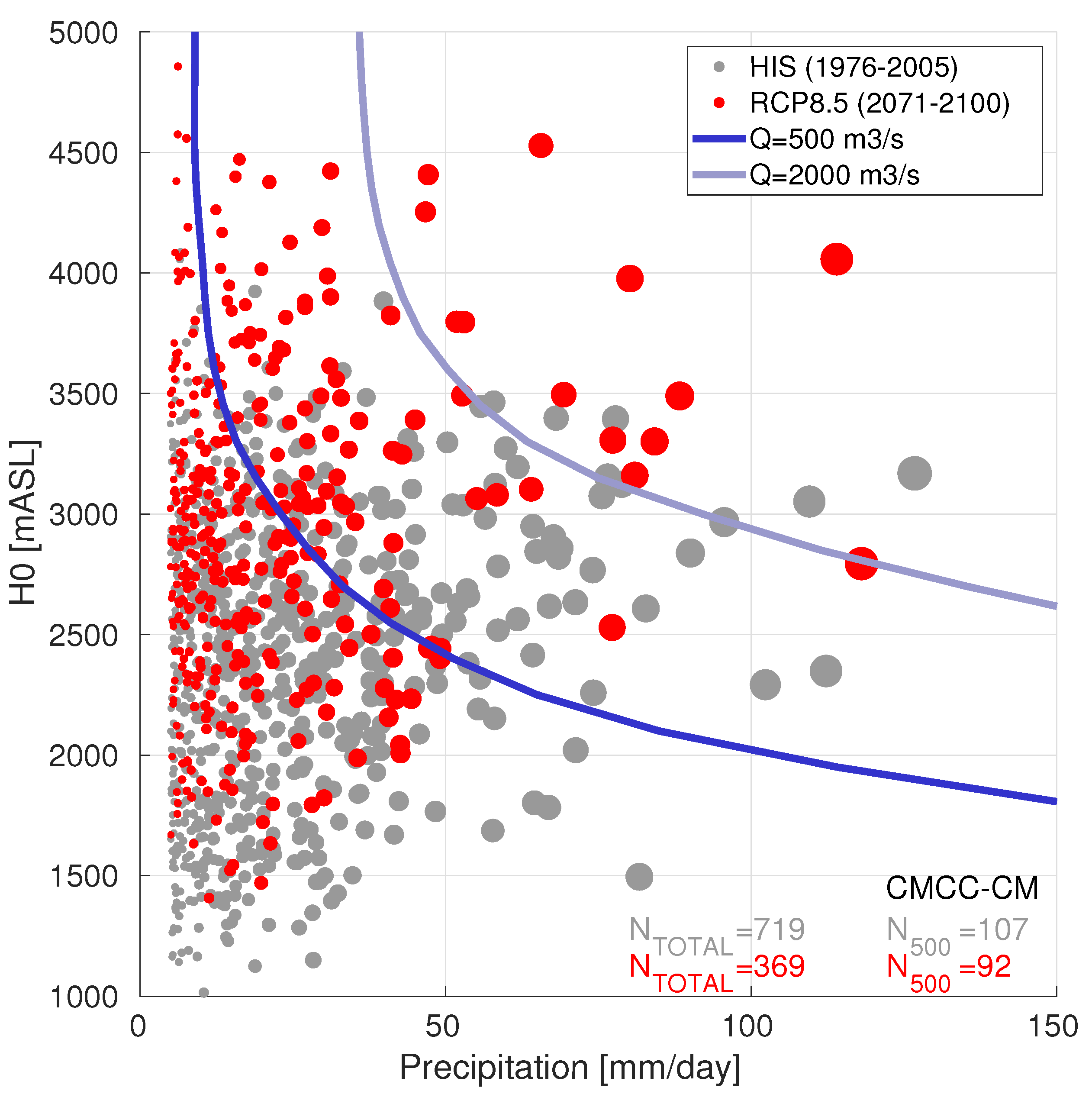
4.3. Hydrological Impact
5. Conclusions
Author Contributions
Funding
Acknowledgments
Conflicts of Interest
References
- Hobbs, P.V.; Easter, R.C.; Fraser, A.B. A theoretical study of the flow of air and fallout of solid precipitation over mountainous terrain: Part II. Microphysics. J. Atmos. Sci. 1973, 30, 813–823. [Google Scholar] [CrossRef] [Green Version]
- White, A.B.; Gottas, D.J.; Strem, E.T.; Ralph, F.M.; Neiman, P.J. An automated brightband height detection algorithm for use with Doppler radar spectral moments. J. Atmos. Ocean. Technol. 2002, 19, 687–697. [Google Scholar] [CrossRef] [Green Version]
- Fabry, F.; Zawadzki, I. Long-term radar observations of the melting layer of precipitation and their interpretation. J. Atmos. Sci. 1995, 52, 838–851. [Google Scholar] [CrossRef]
- Lundquist, J.D.; Neiman, P.J.; Martner, B.; White, A.B.; Gottas, D.J.; Ralph, F.M. Rain versus snow in the Sierra Nevada, California: Comparing Doppler profiling radar and surface observations of melting level. J. Hydrometeorol. 2008, 9, 194–211. [Google Scholar] [CrossRef] [Green Version]
- Cui, G.; Bales, R.; Rice, R.; Anderson, M.; Avanzi, F.; Hartsough, P.; Conklin, M. Detecting Rain-Snow- Transition Elevations in Mountain Basins Using Wireless Sensor Networks. J. Hydrometeorol. 2020, 21, 2061–2081. [Google Scholar] [CrossRef]
- Medina, S.; Smull, B.F.; Houze, R.A., Jr.; Steiner, M. Cross-barrier flow during orographic precipitation events: Results from MAP and IMPROVE. J. Atmos. Sci. 2005, 62, 3580–3598. [Google Scholar] [CrossRef] [Green Version]
- Minder, J.R.; Durran, D.R.; Roe, G.H. Mesoscale controls on the mountainside snow line. J. Atmos. Sci. 2011, 68, 2107–2127. [Google Scholar] [CrossRef]
- Marwitz, J.D. Deep orographic storms over the Sierra Nevada. Part I: Thermodynamic and kinematic structure. J. Atmos. Sci. 1987, 44, 159–173. [Google Scholar] [CrossRef] [Green Version]
- Garreaud, R. Warm winter storms in Central Chile. J. Hydrometeorol. 2013, 14, 1515–1534. [Google Scholar] [CrossRef]
- Ibañez, M.; Gironás, J.; Oberli, C.; Chadwick, C.; Garreaud, R.D. Daily and seasonal variation of the surface temperature lapse rate and 0 °C isotherm height in the western subtropical Andes. Int. J. Climatol. 2020. [Google Scholar] [CrossRef]
- Sumargo, E.; Cannon, F.; Ralph, F.M.; Henn, B. Freezing level forecast error can consume reservoir flood control storage: Potentials for Lake Oroville and New Bullards Bar reservoirs in California. Water Resour. Res. 2020, 56, e2020WR027072. [Google Scholar] [CrossRef]
- Fehlmann, M.; Gascón, E.; Rohrer, M.; Schwarb, M.; Stoffel, M. Estimating the snowfall limit in alpine and pre-alpine valleys: A local evaluation of operational approaches. Atmos. Res. 2018, 204, 136–148. [Google Scholar] [CrossRef]
- Schauwecker, S.; Rohrer, M.; Huggel, C.; Endries, J.; Montoya, N.; Neukom, R.; Perry, B.; Salzmann, N.; Schwarb, M.; Suarez, W. The freezing level in the tropical Andes, Peru: An indicator for present and future glacier extents. J. Geophys. Res. Atmos. 2017, 122, 5172–5189. [Google Scholar] [CrossRef]
- Garreaud, R.; Rutllant, J. Análisis meteorológico de los aluviones de Antofagasta y Santiago de Chile en el periodo 1991–1993. Atmósfera 1996, 9, 251–271. [Google Scholar]
- Liu, A.; Mooney, C.; Szeto, K.; Thériault, J.; Kochtubajda, B.; Stewart, R.; Boodoo, S.; Goodson, R.; Li, Y.; Pomeroy, J. The June 2013 Alberta catastrophic flooding event: Part 1—Climatological aspects and hydrometeorological features. Hydrol. Process. 2016, 30, 4899–4916. [Google Scholar] [CrossRef] [Green Version]
- Cohen, J.; Ye, H.; Jones, J. Trends and variability in rain-on-snow events. Geophys. Res. Lett. 2015, 42, 7115–7122. [Google Scholar] [CrossRef] [Green Version]
- Grote, T. A synoptic climatology of rain-on-snow flooding in Mid-Atlantic region using NCEP/NCAR Re-Analysis. Phys. Geogr. 2020, 1–20. [Google Scholar] [CrossRef]
- Musselman, K.N.; Lehner, F.; Ikeda, K.; Clark, M.P.; Prein, A.F.; Liu, C.; Barlage, M.; Rasmussen, R. Projected increases and shifts in rain-on-snow flood risk over western North America. Nat. Clim. Chang. 2018, 8, 808–812. [Google Scholar] [CrossRef]
- Barnett, T.P.; Adam, J.C.; Lettenmaier, D.P. Potential impacts of a warming climate on water availability in snow-dominated regions. Nature 2005, 438, 303. [Google Scholar] [CrossRef]
- Hatchett, B.J.; Daudert, B.; Garner, C.B.; Oakley, N.S.; Putnam, A.E.; White, A.B. Winter snow level rise in the northern Sierra Nevada from 2008 to 2017. Water 2017, 9, 899. [Google Scholar] [CrossRef] [Green Version]
- Sepúlveda, S.A.; Padilla, C. Rain-induced debris and mudflow triggering factors assessment in the Santiago cordilleran foothills, Central Chile. Nat. Hazards 2008, 47, 201–215. [Google Scholar] [CrossRef]
- Poveda, G.; Espinoza, J.C.; Zuluaga, M.D.; Solman, S.A.; Garreaud Salazar, R.; van Oevelen, P.J. High impact weather events in the Andes. Front. Earth Sci. 2020. [Google Scholar] [CrossRef]
- Viale, M.; Garreaud, R. Orographic effects of the subtropical and extratropical Andes on upwind precipitating clouds. J. Geophys. Res. Atmos. 2015, 120, 4962–4974. [Google Scholar] [CrossRef]
- Falvey, M.; Garreaud, R. Wintertime precipitation episodes in central Chile: Associated meteorological conditions and orographic influences. J. Hydrometeorol. 2007, 8, 171–193. [Google Scholar] [CrossRef]
- Viale, M.; Valenzuela, R.; Garreaud, R.D.; Ralph, F.M. Impacts of atmospheric rivers on precipitation in southern South America. J. Hydrometeorol. 2018, 19, 1671–1687. [Google Scholar] [CrossRef]
- Valenzuela, R.A.; Garreaud, R.D. Extreme daily rainfall in central-southern Chile and its relationship with low-level horizontal water vapor fluxes. J. Hydrometeorol. 2019, 20, 1829–1850. [Google Scholar] [CrossRef]
- Cortés, G.; Vargas, X.; McPhee, J. Climatic sensitivity of streamflow timing in the extratropical western Andes Cordillera. J. Hydrol. 2011, 405, 93–109. [Google Scholar] [CrossRef]
- Rojas, O.; Mardones, M.; Arumí, J.L.; Aguayo, M. Una revisión de inundaciones fluviales en Chile, período 1574–2012: Causas, recurrencia y efectos geográficos. Rev. Geogr. Norte Gd. 2014, 177–192. [Google Scholar] [CrossRef] [Green Version]
- Ayala, L.; López, A.; Tamburrino, A.; Vera, G. Aspectos hidrometeorológicos e hidrodinámicos de algunos eventos aluvionales recientes en Chile. XVI Congr. Latinoam. Hidrául. 1994, 3, 39–51. [Google Scholar]
- Sepúlveda, S.A.; Rebolledo, S.; Vargas, G. Recent catastrophic debris flows in Chile: Geological hazard, climatic relationships and human response. Quat. Int. 2006, 158, 83–95. [Google Scholar] [CrossRef]
- González, S.; Garreaud, R. Spatial variability of near-surface temperature over the coastal mountains in southern Chile (38 S). Meteorol. Atmos. Phys. 2019, 131, 89–104. [Google Scholar] [CrossRef]
- National Geophysical Data Center. 2-minute Gridded Global Relief Data (ETOPO2) v2. National Geophysical Data Center, NOAA. Available online: https://www.ngdc.noaa.gov/mgg/global/etopo2.html (accessed on 25 May 2019).
- Alvarez-Garreton, C.; Mendoza, P.A.; Boisier, J.P.; Addor, N.; Galleguillos, M.; Zambrano-Bigiarini, M.; Lara, A.; Cortes, G.; Garreaud, R.; McPhee, J.; et al. The CAMELS-CL dataset: Catchment attributes and meteorology for large sample studies-Chile dataset. Hydrol. Earth Syst. Sci. 2018, 22, 5817–5846. [Google Scholar] [CrossRef] [Green Version]
- Saha, S.; Moorthi, S.; Pan, H.L.; Wu, X.; Wang, J.; Nadiga, S.; Tripp, P.; Kistler, R.; Woollen, J.; Behringer, D.; et al. The NCEP climate forecast system reanalysis. Bull. Am. Meteorol. Soc. 2010, 91, 1015–1058. [Google Scholar] [CrossRef]
- Taylor, K.E.; Stouffer, R.J.; Meehl, G.A. An overview of CMIP5 and the experiment design. Bull. Am. Meteorol. Soc. 2012, 93, 485–498. [Google Scholar] [CrossRef] [Green Version]
- Center for Climate and Resilience Research, (CR)2 (FONDAP 15110009). Regional Climate Simulations. Available online: http://simulaciones.cr2.cl/ (accessed on 15 May 2019).
- Mardones Bascuñan, P.B. Impactos del Cambio Climático en la Altura de la Isoterma 0 °C Sobre Chile Central. Master’s Thesis, University of Chile, Santiago, Chile, 2019. [Google Scholar]
- Riahi, K.; Rao, S.; Krey, V.; Cho, C.; Chirkov, V.; Fischer, G.; Kindermann, G.; Nakicenovic, N.; Rafaj, P. RCP 8.5—A scenario of comparatively high greenhouse gas emissions. Clim. Chang. 2011, 109, 33. [Google Scholar] [CrossRef] [Green Version]
- Moss, R.H.; Edmonds, J.A.; Hibbard, K.A.; Manning, M.R.; Rose, S.K.; Van Vuuren, D.P.; Carter, T.R.; Emori, S.; Kainuma, M.; Kram, T.; et al. The next generation of scenarios for climate change research and assessment. Nature 2010, 463, 747–756. [Google Scholar] [CrossRef] [PubMed]
- Benarroch, A.; Siles, G.A.; Riera, J.M.; Pérez-Peña, S. Heights of the 0 °C Isotherm and the Bright Band in Madrid: Comparison and Variability. In Proceedings of the 2020 14th European Conference on Antennas and Propagation (EuCAP), Copenhagen, Denmark, 15–20 March 2020; pp. 1–5. [Google Scholar]
- Masiokas, M.H.; Villalba, R.; Luckman, B.H.; Le Quesne, C.; Aravena, J.C. Snowpack variations in the central Andes of Argentina and Chile, 1951–2005: Large-scale atmospheric influences and implications for water resources in the region. J. Clim. 2006, 19, 6334–6352. [Google Scholar] [CrossRef]
- Lenderink, G.; Buishand, A.; Van Deursen, W. Estimates of future discharges of the river Rhine using two scenario methodologies: Direct versus delta approach. Hydrol. Earth Syst. Sci. 2007, 11, 1145–1159. [Google Scholar] [CrossRef]
- Ekström, M.; Jones, P.; Fowler, H.; Lenderink, G.; Buishand, T.; Conway, D. Regional climate model data used within the SWURVE project 1: Projected changes in seasonal patterns and estimation of PET. Hydrol. Earth Syst. Sci. 2007, 11, 1069–1083. [Google Scholar] [CrossRef]
- Zazulie, N.; Rusticucci, M.; Raga, G.B. Regional climate of the Subtropical Central Andes using high-resolution CMIP5 models. Part II: Future projections for the twenty-first century. Clim. Dyn. 2018, 51, 2913–2925. [Google Scholar] [CrossRef]
- Bustos Cavada, D. Cambio climático y eventos de emergencia en el suministro de agua potable en el gran Santiago. Bachelor’s Thesis, University of Chile, Santiago, Chile, 2011. [Google Scholar]
- Bozkurt, D.; Rojas, M.; Boisier, J.P.; Valdivieso, J. Projected hydroclimate changes over Andean basins in central Chile from downscaled CMIP5 models under the low and high emission scenarios. Clim. Chang. 2018, 150, 131–147. [Google Scholar] [CrossRef]
- Vicuña, S.; Garreaud, R.D.; McPhee, J. Climate change impacts on the hydrology of a snowmelt driven basin in semiarid Chile. Clim. Chang. 2011, 105, 469–488. [Google Scholar] [CrossRef]


| Model | Institution | Variables | Spatial Resolution (lat × lon) | Isobaric Levels (hPa) | Periods |
|---|---|---|---|---|---|
| MPI-ESM-LR | Max Planck Institute for Meteorology, Germany | T, Z, pr, sftlf | 1.865 × 1.875 | 1000, 850, 700, 500, 250, 150, 100, 70, 50, 30, 10, 3, 1, 0.3, 0.1 (15) | |
| MIROC5 | Atmosphere and Ocean Research Institute (University of Tokyo) | T, Z, pr, sftlf | 1.400 × 1.406 | 1000, 850, 700, 500, 250, 100, 50, 10 (8) | |
| CNRM-CM5 | National Center of Meteorological Research, France | T, Z, pr, sftlf | 1.400 × 1.406 | 1000, 850, 700, 500, 250, 100, 50, 10 (8) | 1976–2005 (HIS) 2011–2040 (RCPs) 2041–2070 (RCPs) 2071–2100 (RCPs) |
| MRI-CGCM3 | Meteorological Research Institute, Japan | T, Z, pr, sftlf | 1.121 × 1.125 | 1000, 850, 700, 500, 250, 100, 50, 10 (8) | |
| CMCC-CM | Centro Euro-Mediterraneo sui Cambiamenti Climatici, Italy | T, Z, pr, sftlf | 0.748 × 0.750 | 1000, 850, 700, 500, 250, 100, 50, 10 (8) |
Publisher’s Note: MDPI stays neutral with regard to jurisdictional claims in published maps and institutional affiliations. |
© 2020 by the authors. Licensee MDPI, Basel, Switzerland. This article is an open access article distributed under the terms and conditions of the Creative Commons Attribution (CC BY) license (http://creativecommons.org/licenses/by/4.0/).
Share and Cite
Mardones, P.; Garreaud, R.D. Future Changes in the Free Tropospheric Freezing Level and Rain–Snow Limit: The Case of Central Chile. Atmosphere 2020, 11, 1259. https://doi.org/10.3390/atmos11111259
Mardones P, Garreaud RD. Future Changes in the Free Tropospheric Freezing Level and Rain–Snow Limit: The Case of Central Chile. Atmosphere. 2020; 11(11):1259. https://doi.org/10.3390/atmos11111259
Chicago/Turabian StyleMardones, Piero, and René D. Garreaud. 2020. "Future Changes in the Free Tropospheric Freezing Level and Rain–Snow Limit: The Case of Central Chile" Atmosphere 11, no. 11: 1259. https://doi.org/10.3390/atmos11111259